A Steady Regime of Volume and Heat Transports in the Eastern Arctic Ocean in the Early 21st Century

Mooring observations in the eastern Eurasian Basin of the Arctic Ocean showed that mean 2013–2018 along-slope volume and heat (calculated relative to the freezing temperature) transports in the upper 800 m were 4.8 ± 0.1 Sv (1 Sv = 10⁶ m³/s) and 34.8 ± 0.6 TW, respectively. Volume and heat transports within the Atlantic Water (AW) layer (∼150–800 m) in 2013–2018 lacked significant temporal shifts at annual and longer time scales: averaged over the two periods of mooring deployment in 2013–2015 and 2015–2018, volume transports were 3.1 ± 0.1 Sv, while AW heat transports were 31.3 ± 1.0 TW and 34.8 ± 0.8 TW. Moreover, the reconstructed AW volume transports over longer, 2003–2018, period of time showed strong interannual variations but lacked a statistically significant trend. However, we found a weak positive trend of 0.08 ± 0.07 Sv/year in the barotropic AW volume transport estimated using dynamic ocean topography (DOT) measurements in 2003–2014 – the longest period spanned by the DOT dataset. Vertical coherence of 2013–2018 transports in the halocline (70–140 m) and AW (∼150–800 m) layers was high, suggesting the essential role of the barotropic forcing in constraining along-slope transports. Quantitative estimates of transports and their variability discussed in this study help identify the role of atlantification in critical changes of the eastern Arctic Ocean.

Introduction

In recent decades, the Arctic has experienced dramatic changes in all components of the climate system, including sea ice (Comiso et al., 2017), ocean (Polyakov et al., 2017), and atmosphere (Overland et al., 2019). In the eastern Eurasian Basin (EB) of the Arctic Ocean, those changes are partially linked to anomalous inflows from the sub-Arctic seas (Polyakov et al., 2018). Under the increased influence of Atlantic inflows – the inflows of waters originated in the Atlantic Ocean, the hydrographic conditions in the eastern EB evolve toward those previously unique to the western Nansen Basin – the process Polyakov et al. (2017) termed “atlantification.” In light of these changes, quantifying volume and heat transports associated with these inflows is essential to understanding of the current and future states of the Arctic Ocean. However, well-resolved observational estimates of transports in the Arctic Ocean in general and in the eastern EB in particular are rare. The first attempt given to quantify long-term transports in the eastern EB based on instrumental 2013–2015 observations was made by Pnyushkov et al. (2018). They reported the along-slope net transports in the upper 780-m layer of ∼5.1 Sv (1 Sv = 10⁶ m³/s) with the dominant (∼60%) contribution from the Atlantic Water (AW).

Entering the Arctic Ocean from Fram Strait and the Barents Sea (Figure 1), the warm (potential temperature >0°C) and salty (salinity >34.5) AW is distributed along the deep basin margins at intermediate depths (∼150–800 m) by the Arctic Circumpolar Boundary Current (ACBC; Aksenov et al., 2011). This flow carries an enormous amount of heat (Aagaard and Greisman, 1975) and affects the mid-depth thermal balance of the entire Arctic Ocean. AW heat, however, is isolated from the surface by strong stratification of the halocline layer (HL), usually located within the 70–150-m depth range in the EB. Suppressing turbulent mixing, the strong stratification of the HL constrains heat transfer from the AW layer to the upper ocean and the sea ice (Rudels et al., 1996), but recent studies show that the insulating effect of the HL in the EB is weakening as a consequence of the atlantification (Polyakov et al., 2018).

FIGURE 1

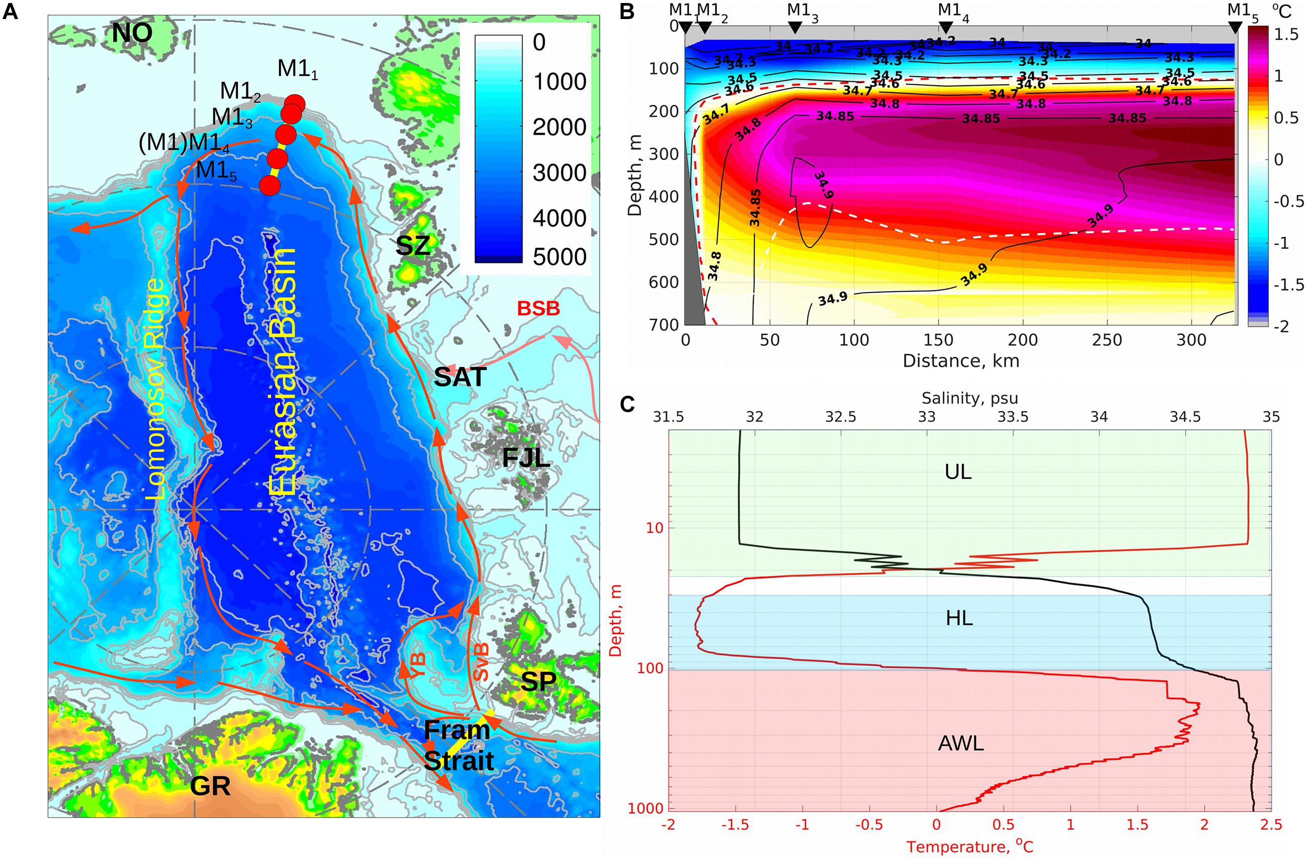
Figure 1. (A) Map showi ng locations of moorings (red circles) over the continental slope of the Laptev Sea in the Eurasian Basin of the Arctic Ocean in 2013–2018. Greenland (GR), Spitsbergen (SP), Franz Joseph Land (FJL), St. Anna Trough (SAT), Severnaya Zemlya (SZ), and Novosibirskiye Islands (NO) are indicated. YB, SvB, and BSB indicate Yermak, Svalbard, and Barents Sea branches of the Atlantic Water (AW), respectively. Red arrows show a schematic pattern of AW circulation in the Eurasian Basin. Bottom depth in meters is shown by color and gray contours (5000, 4000, 3000, 2000, 1000, 800, 600, 400, and 200 m). Sections and moorings used in this study are indicated by yellow segments and red circles. (B) The 2013–2018 mean temperature (color) and salinity (isolines) distributions along the 125°E section. Gray areas at the cross-slope section indicate layers not covered by mooring-based temperature and salinity observations. Black triangles show the position of NABOS moorings. The dashed red line shows the position of the AW layer boundary identified by 0°C isotherm. The dashed white line shows the position of the potential density σ = 27.97. (C) Summer CTD temperature and salinity profiles at the M1₄ mooring site in 2018. AWL, HL, and UL show the AW, halocline, and upper layers, respectively.

In this study, we estimate along-slope transports in the eastern EB using a collection of 2013–2018 mooring observations, which extends previously made estimates for a 2-year period of 2013–2015 (Pnyushkov et al., 2018). In addition, we complement this analysis with estimates of volume transports restored from repeated single mooring observations at the same location using a regression relationship extending temporal coverage of the discussed transport series back in time to 2003.

Data

Mooring Data

In this study, we utilized observations from a cross-slope array of oceanographic moorings deployed in the EB of the Arctic Ocean along the 125°E meridian over two cycles of deployment in 2013–2015 (moorings with an “a” index) and 2015–2018 (moorings with a “b” index; Table 1). A majority of the hydrographic observations in this data set were collected by the Nansen and Amundsen Basins Observational System (NABOS) program at five moorings distributed across the Laptev Sea continental slope (Figure 1A). They were unevenly distributed across the continental slope to capture major features of the ACBC structure with the shallowest mooring located at ∼250-m depth (M1₁ mooring) and the deepest M1₅ mooring located at ∼3400-m depth. The distances between moorings vary from 11 km at the upper slope to 171 km at the deepest part of the section (Figure 1), that exceeds the typical Rossby radius of 7 km for the eastern EB (Nurser and Bacon, 2014). This resolution is sufficient to describe a large-scale pattern of the along-slope flow and associated transports, but is limited in its ability to resolve mesoscale features of those transports.

TABLE 1

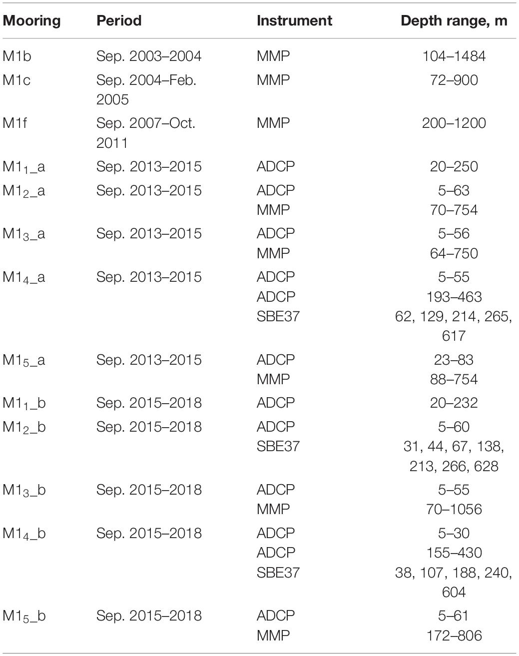
Table 1. Summary of NABOS moorings used in this study.

Oceanographic moorings were equipped with instruments measuring horizontal velocities, temperatures, and conductivities in the ocean layer from the surface to the lower AW boundary at ∼800 m (Supplementary Figure 1). All instruments used at moorings were calibrated by their manufacturers before deployment. Horizontal velocities were measured using two types of devices: McLane Moored Profilers (MMPs) and Acoustic Doppler Current Profilers (AD). The MMPs operated at moorings M1₂, M1₃, and M1₅ between ∼80 and ∼800 m depths (except the MMP at M1₃ in 2015–2018, when it profiled to ∼1100 m) with a vertical resolution of ∼0.25 m and a 2-day interval between profiles.

Current velocities in the upper layer from ∼55–80 m to the surface were sampled with upward-looking ADCPs. Those measurements were collected using the 300-kHz ADCPs at all moorings except M1₁, where a 75-kHz instrument deployed near the bottom was used. At mooring M1₄ a 75-kHz ADCP instrument was used to measure velocities in the layer between 180 and 450 m.

The vertical resolution of the 2013–2018 ADCP records was 2 and 5 meters for the 300 and 75-kHz ADCPs, respectively. However, due to the interference of acoustic signals and instrumental side-lobe contamination near the ocean surface, velocity measurements within the uppermost 10-m layer and inside the nearest to the acoustic ADCP transducer cells were eliminated from our analysis.

For each mooring, MMP and ADCP records were merged forming one dataset that was further used to calculate water and heat transports. Following Pnyushkov et al. (2018), we used ADCP records with a daily temporal resolution, which were filtered using a low-pass filter with a cut-off period of 24 h. Bi-daily MMP profiles were linearly interpolated in time to fit the temporal resolution of the filtered ADCP records. The use of velocity records with different temporal resolutions (low-passed ADCP and snapshot MMP) results in insignificant (<5%) difference of the annual net water transport estimates (Pnyushkov et al., 2018). In the merged dataset, each of the velocity profiles was accompanied by temperature and salinity profiles collected by the MMP and Sea-Bird Electronics (SBE-37) instruments. Existing gaps in temperature, salinity, and velocity profiles in the layers between instruments were filled in using vertical linear interpolation.

In addition to the 2013–2018 data set, we used 2003–2011 velocity, temperature, and salinity measurements at mooring M1, whose location coincides with the position of M1₄ mooring in 2013–2018 (Figure 1 and Table 1). The mooring M1 was equipped with MMP instruments targeted to measure velocity and water properties profiles within the AW layer between ∼100 and 800 m with daily or bi-daily sampling rates. The length of the continuous MMP records at M1 varied from 5 months in 2004–2005 to 3 years in 2008–2011. We summarize details on all moorings used in this study in Table 1.

Original MMP data, including those collected from the 2003–2011 period, were processed using Woods Hole Oceanographic Institution software and then averaged over 2 dbar pressure bins to reduce the effects of small-scale variability in velocity profiles. According to the manufacturer’s manual, an instrumental error of the acoustic current meter (ACM) installed at MMPs is ±0.5 cm s^–1. The instrumental accuracy of the MMP magnetic compass is 2°. The manufacturer’s estimate for the accuracy of speed measurements made with 300− and 75-kHz ADCPs are less than 1 cm s^–1 for velocity profiles averaged over 50 individual ensembles, and 2° for current direction. However, due to the weak horizontal component of the geomagnetic field in the Arctic Ocean, the individual compass error may exceed the instrumental accuracy, reaching 30° (Thurnherr et al., 2017). Despite the potentially large uncertainty in current directions, a comparison of velocities measured by different ADCP and MMP instruments at close levels shows good agreement for speed and directions between the current records with high (in the range from 0.4 to 0.8) correlations (see Iarc Technical Report, 2018).

Dynamic Ocean Topography

We complement our analysis of mooring-based transports along the Laptev Sea slope with estimates of barotropic transports for the same segment of the slope using a dataset of Arctic Dynamic Ocean Topography (DOT). Those monthly DOT observations were obtained from satellite-based radar altimetry combined with Gravity Recovery and Climate Experiment (GRACE) ocean mass measurements described in detail by Armitage et al. (2016). These data are limited from the north by 81.5°N latitude and available for the eastern EB at a regular spherical grid with a spatial resolution of 0.25 × 0.5 degrees by latitude and longitude, respectively. The temporal coverage of this dataset is from 2003 to 2014 that provides substantial overlap with our instrumental observations for comparison.

Materials and Methods

The methods used for the calculation of water (in terms of volume transport in units of m³/s or Sv) and heat transports, and heat transport density are described in Supplementary Section 1 and more details in Pnyushkov et al. (2018). Here we provide important details on those calculations.

Depth-Integrated Transports

Depth-integrated water and heat transports (or transports per unit section width) at moorings were calculated by vertical integration of the eastward velocities and the products of the eastward velocities and temperature anomaly T(z)-T_ref, where T_ref = –1.8°C is the freezing point. For calculations of the AW depth-integrated transports, the shallowest and deepest levels with positive water temperatures (T > 0°C) were determined and then used as depth limits.

Along-Slope Transports

The along-slope volume and heat transports through the Laptev Sea mooring section (Figure 1) were estimated by integrating the depth-integrated transports horizontally over the length of the mooring transect. The employed method of integration is equivalent to the implementation of linear interpolation to restore depth-integrated transports in the cross-slope direction. The unclosed (non-zero) volume balance, when the advected mass is not conserved, makes the results of heat transport calculations sensitive to the choice of T_ref (Schauer and Beszczynska-Möller, 2009). To address this problem, we additionally evaluate heat transport density – the amount of heat transported by a unit of volume transport. This quantity was calculated as a ratio of the heat and volume transports; it shows the amount of heat transported by a water transport of 1 Sv (see Supplementary Section 1 for details). More generally, it quantifies the heat content transported by the mean current and can be used for the assessment of temporal variability of the heat transports (Pnyushkov et al., 2018).

The volume and heat transports were estimated separately for the upper (UL), HL, and AW layer (Figure 1C). In the paper, we define the UL as a water layer between the 10- and 40-m depths which corresponds to the depths of the current profilers covering the upper ocean layer. The HL lies below the UL and spreads from 70 to 140-m depths (Figure 1C). The upper and lower boundaries of the AW layer were identified by the depth of 0 °C isotherms; they vary between moorings and over seasons, with means corresponding to ∼80 and ∼800 m depth, respectively.

Results

Cross-Slope Current Structure and Vertical Flow Coherence

The spatial structure of the ACBC in 2013–2018 reveals a gradual decrease of current velocities seaward across the continental slope (Figure 2A). This decrease agrees well with the velocity pattern documented for the Laptev Sea slope using 2005–2015 instrumental observations (Pnyushkov et al., 2018) and modeling (Aksenov et al., 2011). In 2013–2018 the most energetic currents within the 0–800 m layer were found at mooring M1₂, where they reached 9.5 cm/s; at the shallowest mooring, M1₁, the mean current speed of 9.3 cm/s was comparable, but observations at this mooring were limited to the deepest observational level of ∼260 m. Mean currents at the two deep moorings M1₄ and M1₅ in 2013–2018 are an order of magnitude weaker, reaching only ∼1.5 and ∼0.1 cm/s, respectively (Figure 2A). Daily velocities at these moorings demonstrate substantial variability both in amplitudes and directions (not shown), which suggests that the topographic control of barotropic flow may not be as strong as for the upper slope moorings where bottom depth and sea surface height gradients are larger.

FIGURE 2

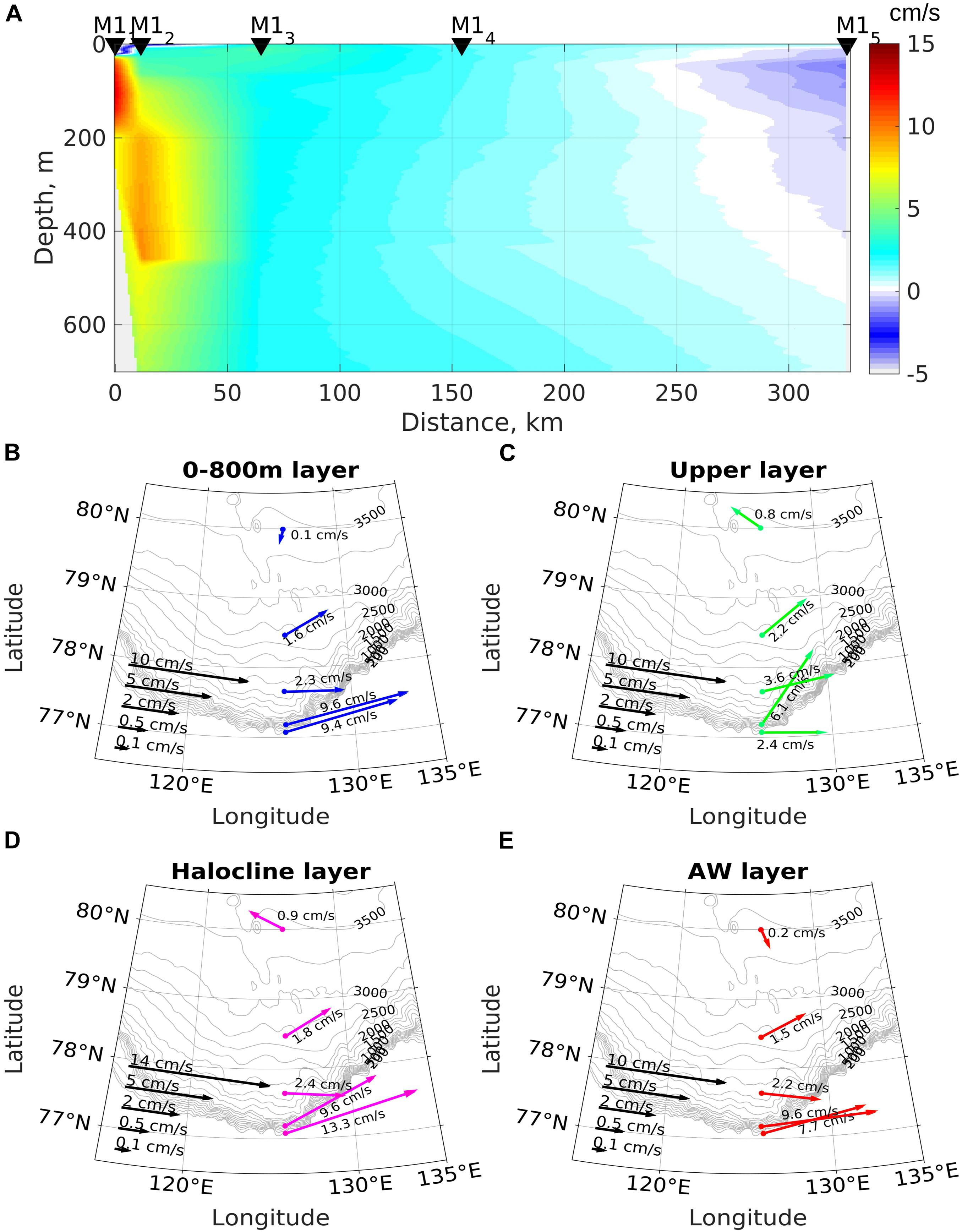
Figure 2. Averaged over 2013–2018 eastward velocities (A) and current vectors (B–E) derived from mooring observations at the Laptev Sea slope in the upper 800-m layer (B), in the upper 40-m layer (C), in the halocline (70–140 m) layer (D), and in the AW layer (E). Note that a non-linear scale was used to plot vectors.

Vertical coherence of currents was evaluated by averaging currents in the upper ocean, halocline, and AW layers. For each layer, we calculated the 2013–2018 mean velocities shown in Figure 2. For all moorings, mean currents in the halocline and the AW layers were strongly coherent following the same direction generally aligned to isobaths (Figure 2). This conclusion is corroborated by the vector correlation (R_vec; Hanson et al., 1992) between time series of daily velocity vectors averaged in those layers; at all moorings correlation was high varying from 0.58 at mooring M1₅ to 0.86 at mooring M1₄. This high coherence of the flow in the HL and AW layer is likely a consequence of topographically-controlled flow due to potential vorticity conservation. The coherence of the flow within the HL and the UL is weaker and varies from a moderate R_vec = 0.31 at M1₅ to a rather high R_vec = 0.83 at M1₂. The largest difference of directions of the mean currents in the UL and HL never exceeded 30° at M1₂ mooring; at deeper mooring locations, the difference was lower, never exceeding 17°. The only exception was the deepest mooring M1₅, where weak currents in 2013–2018 did not have persistent current direction in the intermediate and deep layers such that their vertical coherence was not statistically robust. Together, the high vertical coherence and significant correlation between transports within the HL and AW layer at annual temporal scales suggest that the flow is essentially barotropic.

Volume Transports in 2013–2018

In the upper 800-m layer, the largest (up to 150 m²/s) depth-integrated transport was estimated at mooring M1₂ (Figure 3A). Despite comparable mean eastward velocity at the neighboring mooring M1₁ (compare 8.7 cm/s at the M1₁ site and 7.2 cm/s at the M1₂ mooring; Figure 2A), the depth-integrated transport there was smaller (<65 m²/s) due to the shallower water depth. Replicating the cross-slope pattern of the mean eastward velocity, the depth-integrated transports progressively decrease from the M1₂ mooring site toward the deep part of the section (Figure 3A). At the deepest mooring the weakening of the eastward transports was accompanied by changes of flow direction so that the transports in the upper 800 m and the AW layers become negative (westward) during a substantial part of the time in 2013–2018 (Figures 3A,B).

FIGURE 3

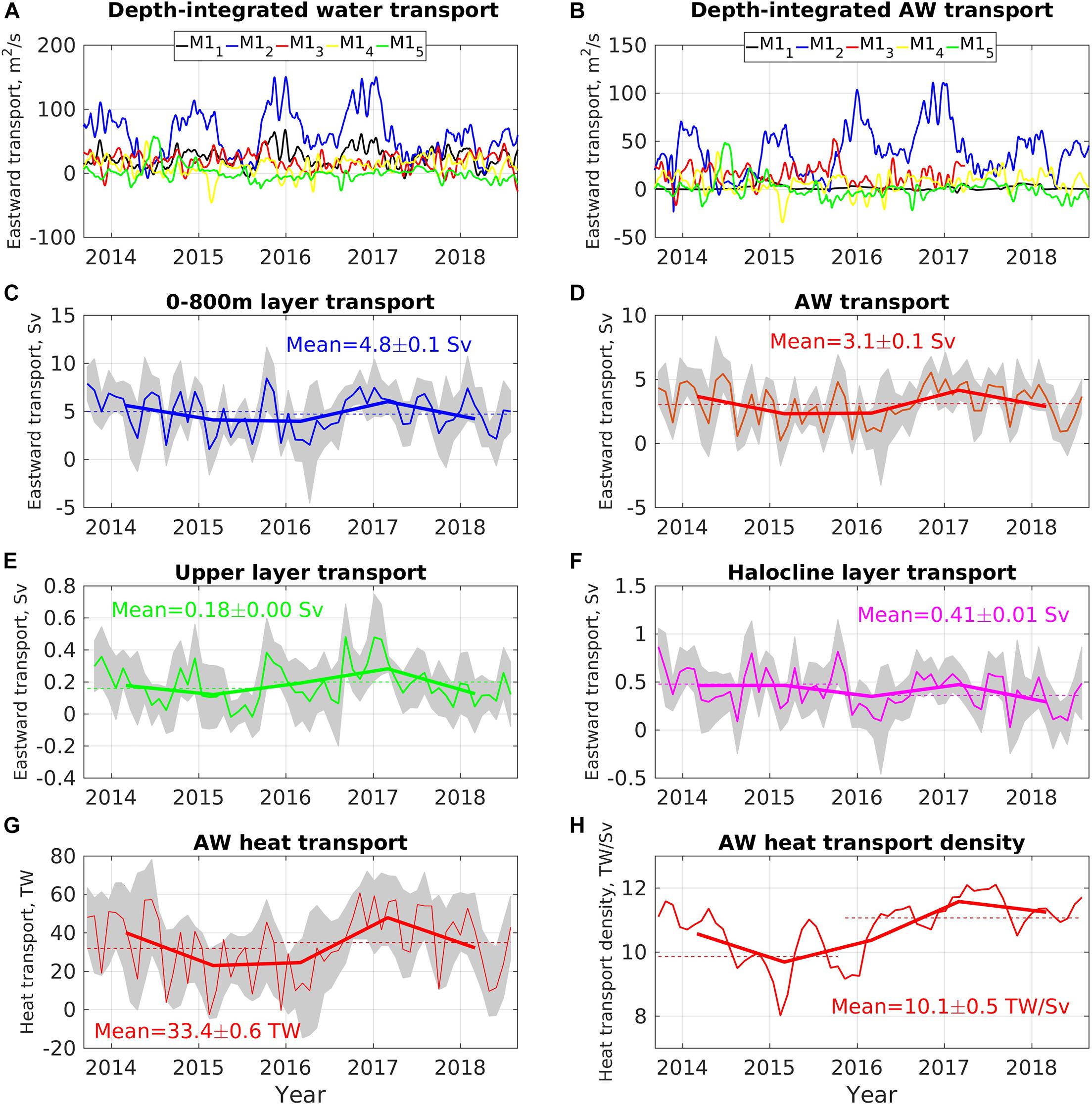
Figure 3. Depth-integrated transports (A) in the upper 800-m layer and (B) in the AW layer. Monthly net volume transport across the Laptev Sea slope (C) in the upper 800-m layer, (D) in the AW layer, (E) in the UL (10–40 m) and (F) in the HL (70–140 m). Monthly heat transport (G) and heat transport density (H) in the AW layer across the 125E section in 2013–2018. Dashed lines in (C,D) show the 2013–2015 and 2015–2018 means. Gray areas in (C,G) represent one standard deviation intervals.

Depth-integrated transports demonstrated substantial seasonality with amplitudes of the seasonal signal varying across the slope. Within the upper 800-m layer, the strongest seasonal signal in depth-integrated transports was observed at the M1₂ mooring site reaching ∼140 m²/s in 2015–2016 (Figure 3A). The transports typically peak in December-January decreasing to several tens of m²/s in the summer months. A similar pattern of the seasonal cycle is evident for the depth-integrated transports in the AW layer (Figure 3B). Pnyushkov et al. (2018) found that the amplitudes of seasonal changes of water transport reduce toward the deep Laptev Sea slope, so that the relative contribution of the seasonal signal to the total depth-integrated transport variability changes from dominant (>50%) at shallow moorings to less than 11% at the relatively deep mooring M1₄.

Using calculated depth-integrated transports at individual moorings, we estimated net transports and the relative contribution of transports between moorings to the net transport across the entire Laptev Sea section. The 2013–2018 transports in the upper 800-m and AW layers were 4.8 and 3.1 Sv, respectively (Table 2). For the upper 800-m layer, the transport between M1₂ and M1₃ was the largest contributor, accounting for over 44.5% of the net volume transport (Table 3). Since the AW occupies up to 90% of the upper 800-m, the contribution from this mooring segment to the AW volume transport was also high (45.4%). Because the most energetic currents are found over the upper part of the EB continental slope, the three shallowest moorings M1₁, M1₂, and M1₃ contributed >50% to the net volume transport across the section in both 800-m and AW layers.

TABLE 2

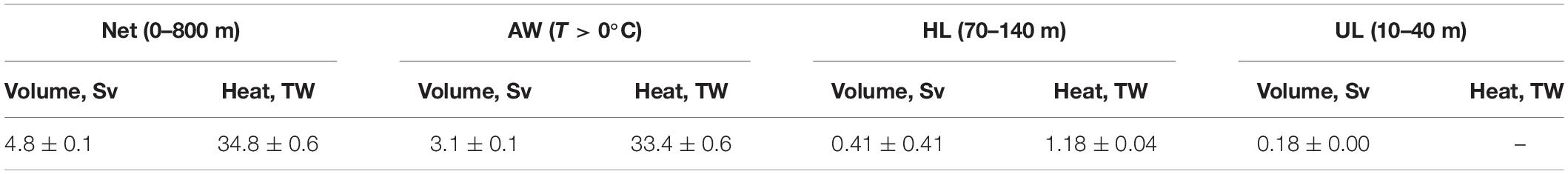
Table 2. Mean volume and heat transports across the Laptev Sea section in the upper ∼800 m (Net), Atlantic Water (AW), halocline (HL), and upper ocean (UL) layers in 2013–2018.

TABLE 3

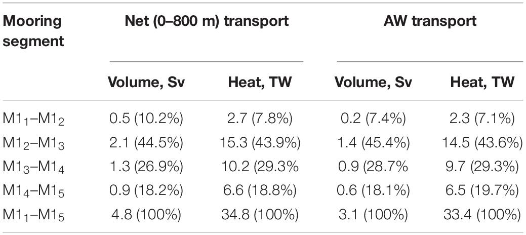
Table 3. Transports between moorings and their relative contributions (numbers in brackets) to the net volume and heat transports across the Laptev Sea section in the upper ∼800 m and AW layers.

The limited length (5 years) of the available records with substantial seasonal and year-to-year variations prevents meaningful estimates of statistical trends in the volume transports. As an alternative, we calculated transports averaged over extended (from one to several years) periods of time (Table 4). We found that year-to-year variations of AW volume transports are strong, ranging from 2.3 Sv in 2014–2015 to 4.2 Sv in 2016–2017, indicating almost doubling of the AW volume transports in some years (Table 4 and Figure 3D). Thus, interannual variability is one of the dominant modes of the along-slope transport variability at the eastern EB continental slope. However, AW volume transports averaged over 2013–2015 and 2015–2018 were both ∼3.1 Sv. For the entire upper 800-m layer including AW, HL and UL, the 2015–2018 transport was ∼0.5 Sv weaker compared to the transport in 2013–2015. Figure 3F suggests the weakening of volume transport in the HL over 2013–2018 (from 0.46 Sv in 2013–2015 to 0.38 Sv in 2015–2018), thus partially explaining the overall reduction of the along-slope volume transport in the upper 800 m.

TABLE 4

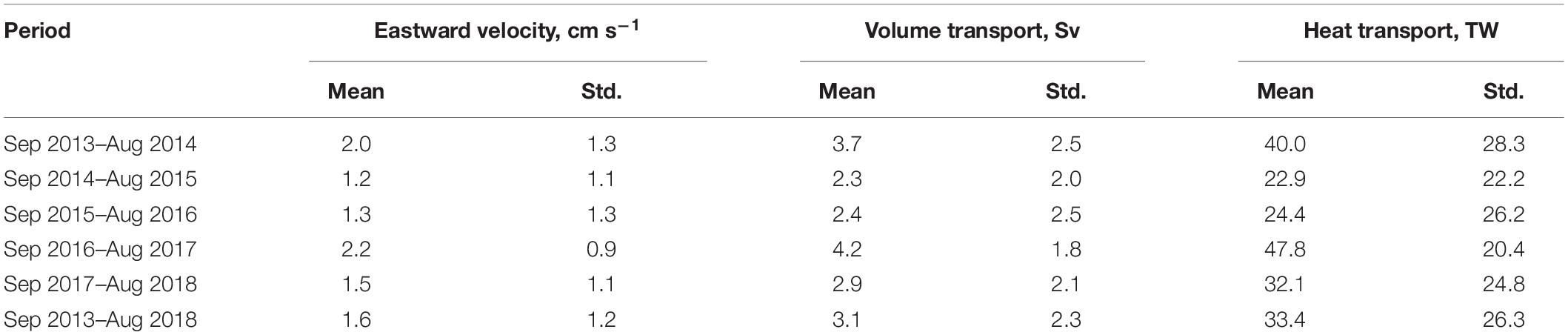
Table 4. Means and standard deviations (Std) of the eastward volume and heat transports in the AW layer across the Laptev Sea slope estimated from mooring observations in 2013–2018.

The vertical overlap and gaps between the UL, HL, and AW layer result in unbalanced volume transports in those three layers and the net transport in the upper 800-m layer (Figure 3C) since the sum of the UL, HL, and AW layer transports is not necessarily equal to the upper 800-m layer transport. To estimate the sensitivity of the calculated transports to this imbalance, we additionally calculated transports for the three layers with fixed boundaries (specifically, for the 10–40, 40–130, and 130–800 m layers; Figure 4). The boundary between the two deepest layers (130 m) matches the average position of the upper AW boundary at moorings M1₄ and M1₅ in 2013–2018 determined using a zero degree isotherm.

FIGURE 4

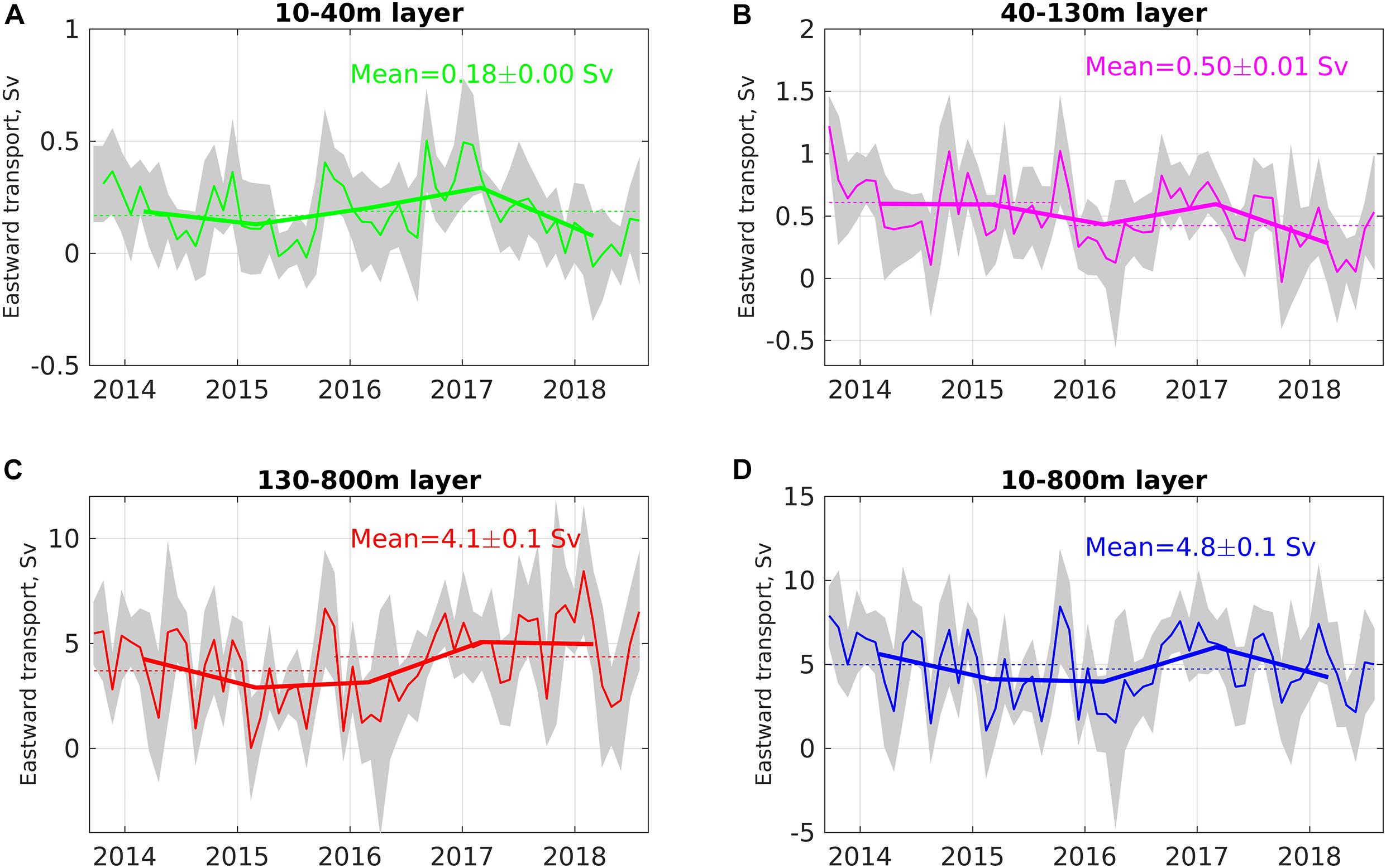
Figure 4. Monthly net volume transport across the Laptev Sea slope (A) in the 10–40 m, (B) 40–130 m, (C) 130–80 m, and (D) in the upper 800-m layer.

The estimated eastward volume transports in the 10–40 m layer increase from 0.17 Sv in 2013–2015 to 0.19 in 2015–2018, reflecting slightly enhanced upper ocean dynamics over the Laptev Sea slope in recent years (Polyakov et al., 2020b). The UL volume transports peaked in 2017 when they reached ∼0.29 Sv (almost doubling the 2013–2015 UL volume transport) but substantially decreased to 0.08 Sv next year. We found that the calculated 40–130 m volume transports in 2013–2018 reflect the essential features of the HL transports (Figure 3F). Averaged over the two periods of mooring deployments in 2013–2018, the 40–130 m volume transport shows a 31% decrease (from 0.61 ± 0.01 Sv in 2013–2015 to 0.42 Sv in 2015–2018), suggesting that our conclusion about the weakening of the HL volume transport is robust. In contrast to the decreased 40–130 m water transport, the volume transport in the 130–800 m layer revealed a 7% increase from 4.0 ± 0.1 Sv to 4.2 ± 0.1 Sv. However, because the AW occupies only a part of the Laptev Sea slope covered by the mooring observations (Figure 1B), transports in the 130–800 m layer are not directly applicable to the assessment of the AW volume transports.

Retrospective Analysis of AW Volume Transports

Using MMP observations from M1 mooring made prior 2011, we reconstructed along-slope transports in the eastern EB for 2003–2011 using regression relationship, thus extending our 2013–2018 estimates back in time for 9 years. This approach was based on the fact that currents at the deeper part of the slope (moorings M1₄ and M1₅) contribute significantly (up to 60%) to the variability of the along-slope transports in the eastern EB (Pnyushkov et al., 2018; Section “Discussion” of this study). In agreement with that, we found that the depth-integrated AW volume transport in 2013–2018 at M1₄ mooring and the AW volume transport across the entire section are well correlated (R = 0.70 ± 0.07). We used this correlation to build a regression relationship between those variables (Figure 5). The root-mean-squared difference (RMSD) between the restored and observed daily series is moderate (1.9 Sv) and dominated by high-frequency component. Therefore, RMSD decreases to ∼0.9 Sv if just a 2-month running-mean smoothing is applied to daily transports.

FIGURE 5

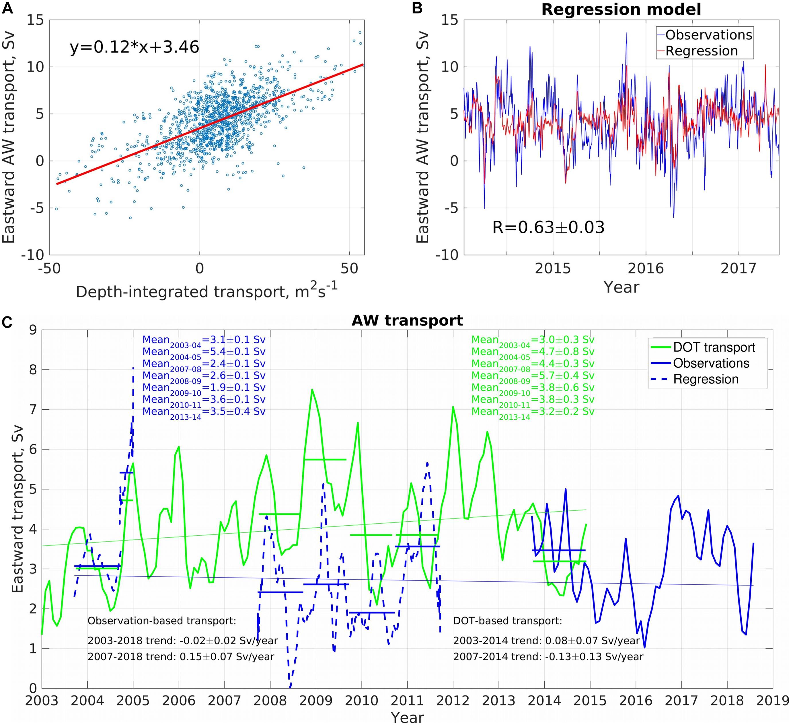
Figure 5. (A) A linear fit between daily depth-integrated transport at mooring M1₄ and the AW volume transport across the Laptev Sea slope in 2013–2018. (B) Daily time series of the observed (blue line) and the restored (red line) AW transports calculated by the linear regression model. R indicates a correlation coefficient. (C) Time series of net barotropic AW volume transport through the central Laptev Sea section estimated from AW volume transport from velocity measurements (blue), and restored using linear regression at M1₄ mooring (blue dashed line) and from DOT data set (green line). Horizontal blue and green lines show annual (averaged from September through August) AW volume transports in 2003–2015 except 2004–2005 when the MMP record was limited to 5 months. The thin blue and green lines show the 2003–2018 observation- and 2003–2014 DOT-based AW volume transport trends, respectively.

The calculated regression relationship for 2013–2018 was used to reconstruct the along-slope AW volume transport extending back to 2003, using AW depth-integrated transports at the M1 mooring site (Figure 5C). Similar to shorter 2013–2015 records (Section “Volume Transports in 2013–2018”), over the entire length of the record (∼15 years) the AW volume transport shows no statistically significant trend (-0.02 ± 0.02 Sv/yr). AW volume transport, however, shows substantial interannual variability. For example, AW volume transport peaked in 2004–2005 exceeding 8 Sv (Figure 5C). Although, we note that 2004–2005 AW volume transport was estimated using the 5-month-long record and, thus, this estimate may be sensitive to seasonal variability of currents. The time period between 2008 and 2010 was exceptional, with dominant small (<1 Sv) and even close to zero in 2008 eastward AW transport. This low transport resulted from the large-scale change of temperature and salinity which modified the geostrophic circulation in the eastern EB in 2008–2011. During this time, the eastward current in the AW layer was, on average, four times weaker compared to 2003–2007 and 2013–2018 (Supplementary Table 1; Pnyushkov et al., 2015).

DOT Volume Transports

In order to assess the role of barotropic component in shaping along-slope transports, we used the geostrophic currents derived from the satellite-based DOT product (Armitage et al., 2016), and calculated along-slope barotropic transports in the AW layer across the same mooring section (Figure 5C). This comparison shows that in 2013–2014 (the period of data overlap with the 2013–2015 deployment of NABOS moorings), the average DOT- and mooring-based AW volume transports differed by ∼0.2 Sv, or less than 6%. The agreement of transports during the period 2003–2011, however, is less evident. In 2003–2005 their means differed insignificantly, by the same 0.2 Sv (or ∼5%) but the difference was substantial in 2008–2010 (Figure 5C). We note that temporal variability of the boundary flow in these years was dominated by anomalous horizontal density gradients (thus the boundary current was significantly affected by baroclinic forcing), resulting in weakened eastward circulation in the eastern EB (Pnyushkov et al., 2015). This baroclinic component of the flow was not captured by DOT observations, resulting in a larger discrepancy between the barotropic DOT- and mooring-based transports. However, the reasonable match of the DOT- and mooring-based transports for other years suggests that a substantial part of the AW volume transport across the Laptev Sea slope in these years was barotropic.

We found a weak positive trend of 0.08 ± 0.07 Sv/year in the barotropic DOT-based AW volume transport in 2003–2014 – the most extended period spanned by the DOT dataset (Figure 5C). Over this period, the barotropic AW volume transport increased by ∼0.9 Sv (or by ∼23% compared to the 2003–2014 mean barotropic AW volume transport of 4.0 Sv). In contrast, the reconstructed mooring-based AW volume transports suggest a negative trend in 2003–2014 (-0.03 ± 0.02 Sv/yr), but demonstrate an increase with a rate of 0.15 ± 0.07 Sv/yr for a shorter period of 2007–2018 (Figure 5C). This 2007–2018 increase was smaller (∼0.5 Sv) compared to that found in the DOT-based AW volume transport, so that the transport increased from 2.6 ± 0.1 Sv (2007–2011 mean AW volume transport) to 3.1 ± 0.1 Sv in 2013–2018.

Substantial interannual variability of the AW volume transports increases the uncertainty of these estimates of trends. For instance, the 2003–2014 trends in the DOT- and mooring-based AW volume transports are close to the edge of the 95% confidence intervals (confidence intervals in this study were estimated using the Student t-test) and, therefore, should be considered with caution. Moreover, annual peaks in the AW volume transports (e.g., in 2004, 2011; Figure 5C) make these estimates sensitive to the specific period for which they are calculated. For example, the positive trend in 2003–2014 in the barotropic DOT-based AW volume transport is changed to a weak negative trend (-0.13 ± 0.13 Sv/year) when considering a shorter period (2007–2015), the beginning of which coincides with the beginning of increased transports based on mooring records (Figure 5C).

Heat Transports in 2013–2018

The thermal state of the Arctic Ocean, to a large degree, is determined by the amount of heat carried by the ACBC within the AW layer (Fahrbach et al., 2001; Schauer et al., 2004). Using our mooring observations, we quantify here heat transports at the Laptev Sea slope.

The contribution of shallow moorings to the AW heat transport dominates (Table 3). For instance, the strongest AW heat transport was estimated for the section segment between the M1₂ and M1₃ moorings. The dominance of shallow moorings both in the volume and heat transports along with weak correlations between the average temperatures within the AW layer and depth-integrated AW transports (the correlation coefficients vary in a range from 0.06 ± 0.06 to 0.31 ± 0.04) indicate that the spatiotemporal pattern of heat transports is formed by currents, with only minor contribution from temperature variations.

2013–2018 mean AW heat transport is estimated as 33.4 ± 0.6 TW. Separated into the two periods of 2013–2015 and 2015–2018, the AW heat transport shows no substantial differences (<10%, Table 4). Specifically, AW heat transport changed from 31.7 TW in 2013–2015 to 34.8 TW in 2015–2018 suggesting a slightly strengthened AW heat advection in the three recent years (Figures 3G,H). However, due to the strong year-to-year variability of those transports compared to the AW heat transport increase and the relatively short length of our records, this finding requires further observations for validation. Moreover, the heat transport shows substantial seasonality likely linked to the seasonality of water temperatures and velocities in the AW layer (not shown), where the seasonal signal at some moorings is strong or even dominant (Baumann et al., 2018). Together with the strong year-to-year variability, seasonal variability makes it difficult to assess the statistical significance of the observed changes in heat transport.

Unbalanced volume transport across the cross-slope section may result in ambiguous interpretation of the heat transport estimates (e.g., Schauer and Beszczynska-Möller, 2009). However, our estimates of the AW volume transport in 2013–2015 and 2015–2018 were fairly close (both are 3.1 ± 0.1 Sv), suggesting that the effect of the unbalanced transport is not significant. Moreover, we found that the heat transport density, which partially addresses the problem of unbalanced volume transports (see Pnyushkov et al., 2018 and also section “Materials and Methods”), changed from 9.8 TW/Sv in 2013–2015 to 11.0 TW/Sv in 2015–2018. These estimates show a 12% increase in 2015–2018 relative to 2013–2015 which is comparable to the 10% increase found using heat transport estimates. Since, arguably, the heat transport density is not sensitive to the volume transport changes, we conclude that our finding of the modest changes of the AW heat transport over 2013–2018 is robust.

Discussion

AW Heat and Volume Transports in the Eastern EB

The estimated 2013–2018 volume transports of 4.8 Sv for the upper 800-m and 3.1 Sv for the AW layers are similar with the estimates for 2013–2015 (Pnyushkov et al., 2018). Since the UL and HL are much thinner than the AW layer, volume transports in these two layers were just ∼6 and ∼13% of the AW transport, respectively (Figures 3E,F). Mooring records show that the heat and volume transports along the Laptev Sea slope in 2013–2018 were steady, with no significant increases or decreases. At longer time scales, we also found no significant trends in the AW volume transports, as evident from the reconstructed series complementing 2013–2018 observations by adding 2003–2011 estimates (Figure 5). There are, however, extended periods when volume transports differ substantially from the 2003–2018 mean. For instance, in 2008–2011 the restored transport was weaker (∼2.6 ± 0.1 Sv) due to anomalous effect of baroclinic forcing. Similar to AW volume transports, the difference between UL transports in 2013–2015 and 2015–2018 was small (<5%). In the HL the volume transport decreased by ∼18% over this period of time; thus, HL was the only layer within the upper 800 m which showed significant change. The main reason for this decrease is a significant weakening of eastern velocities in the halocline layer, observed in the proximity to the hydrographic front – the area of strong lateral density gradients – at mooring M1₂ (see Bauch et al., 2014; Alkire et al., 2017 for details). Depth-integrated transports in the halocline layer at this mooring decreased two times from 6.4 ± 0.2 m²/s in 2013–2015 to 3.2 ± 0.1 m²/s in 2015–2018. At the same time, depth-integrated transport in the upper 800-m layer shows an increase from 55.5 ± 1.5 m²/s to 65.7 ± 1.4 m²/s for two periods of mooring deployments, suggesting an essential role of baroclinic currents in the halocline transport decrease.

Factors Controlling AW Heat Losses on the Way From Fram Strait to the Eastern EB

How can we reconcile our estimates in the eastern EB with those from the upstream locations?

Water Transport

Two major water sources form the ACBC in the eastern Arctic, namely: Fram Strait branch and Barents Sea branch of AW (Aksenov et al., 2011). 1997–2010 measurements in Fram Strait provided an estimate of the AW volume transport of 3.0 ± 0.2 Sv (see Figure 1A for the location; Beszczynska-Möller et al., 2012). A year-long (1991–1992) mooring observations collected at the cross-section between Franz Joseph Land and Severnaya Zemlya provide a rough estimate of 1.9 Sv for the Barents Sea water influx (Loeng et al., 1997). Thus, the total influx of the AW into the Arctic Ocean interior may be roughly estimates as 4.9 Sv. We note that the Barents Sea branch waters are denser that the Fram Strait branch waters so that, upon mixing north of St. Anna Trough, an unknown part of these Barents Sea branch waters sinks to the greater depths below the depth range we consider in this analysis (making our comparative analysis conservative). Thus, the use of this estimate should be viewed as very approximate given that, in addition to the very short record in the Barents Sea, the partitioning of the Barents Sea AW between the depth layers is hard to constrain. Moreover, AW volume transport estimates made for several locations along the EB slope differ significantly. According to Våge et al. (2016), the snapshot AW volume transport in the area to the north of Svalbard was only 1.6 ± 0.3 Sv, differing by ∼1.5 Sv (∼50%) from our 2013–2018 AW volume transport across the 125°E section. Pérez-Hernández et al. (2017) using synoptic-scale cross-slope CTD sections between 21 and 33°E reported along-slope AW volume transport of 2.31 ± 0.29 Sv. Kolås et al. (2020) utilizing CTD data from ship-based surveys and an autonomous underwater glider mission in summer and fall 2018 reported AW volume transport of 3.0 ± 0.2 Sv, with an intraseasonal variability of 1 Sv. The plausible reasons for that wide range of AW volume transport estimates are different time scales of observations used for transport calculations (i.e., synoptic scale at Svalbard and annual scale at the Laptev Sea slopes) concurrent by the strong annual variability of those transports.

Even with all these estimates in hand a direct comparison of transports at different locations is not trivial. For example, AW volume transports across Fram Strait were assessed for the water mass determined by 2°C isotherm whereas in the central Arctic Ocean AW is traditionally bounded by 0°C. In order to make these estimates intercomparable, we assume that the modified AW in the eastern EB occupies the whole upper ocean bounded from below by the depth of potential density σ = 27.97 which corresponds to 2°C isotherm in Fram Strait (Beszczynska-Möller et al., 2012). In making this assumption, we use the fact that UL and HL in the eastern Arctic are occupied by the modified AW, with contribution of AW to the Arctic surface water composition greater than 90–95%. Recalculated for these boundaries, mean volume transport in the eastern EB becomes 3.2 ± 0.1 Sv in 2013–2018. This estimate constitutes ∼67% of the total estimated influx of AW through the eastern Arctic Ocean gateways – a reasonably close match considering uncertainties and assumptions made and possible physical reasons for the loss of AW by the ACBC on its way into the ocean interior.

Heat Transport

Relatively small difference between the AW volume transports at Atlantic gateways to the Arctic Ocean and at the Laptev Sea slope makes possible comparison of the AW heat transports, neglecting the uncertainties due to unclosed mass balance (see Schauer and Beszczynska-Möller, 2009 for details). In that we argue that the main source of AW heat is the AW Fram Strait branch. In Fram Strait, where the mean AW temperature and volume transport are 3.1 ± 0.1°C and 3.0 ± 0.2 Sv, respectively, 1997–2010 AW heat transport can be roughly estimated as 58.8 TW (Beszczynska-Möller et al., 2012). At the Laptev Sea slope, the AW carries ∼33.4 ± 0.6 TW (Table 2), suggesting that the AW loses ∼25 TW on its way along the basin margin from Fram Strait to the eastern EB. In this analysis, we used estimates of heat transports for the AW layer defined by 0°C isotherms since these estimates take into account AW heat defused below σ = 27.97 and the fact that UL and HL carry little AW heat (Table 2).

Using 2007 summer snapshot cross-slope observations made from Franz Josef Land (43°E) through the traverse of Wrangel Island (175°W), Polyakov et al. (2010) estimated that, on average, the upper ocean layer overlying the AW gains approximately 7% of the AW heat losses, assuming that 93% is vented through lateral spread by advection and eddy stirring. If we project the same rate of partitioning between the vertical and lateral dissipation of AW heat, then 1.8 TW out of 25 TW of the total AW heat losses goes to warm HL and UL (and eventually, sea ice melting), whereas 23.2 TW spreads laterally into the deep basin. These vertical (lateral) heat losses are equivalent to 3.1 (1770) W/m² of annual vertical (horizontal) AW heat flux along the 1900-km path from Fram Strait to the central Laptev Sea through a 300-km wide (700-m tall) cross-slope section. This estimate of summer vertical heat flux agrees well with double-diffusive heat fluxes of 3–4 W/m² derived from microstructure observations made in 2007 and 2008 (Polyakov et al., 2019) and 2018 (Schulz et al., 2021) in the eastern EB. Since we compare the heat transports made in different periods and considering the positive AW temperature trend in Fram Strait (0.06°C/year; Beszczynska-Möller et al., 2012), uncertainties of our estimates are high and the actual vertical AW heat loss may be greater.

Uncertainty of the estimates of the rates of AW ventilation is related to the sensitivity of heat transports to the choice of T_ref. This uncertainty is large and may be comparable to the magnitude of the signal itself (e.g., Schauer and Beszczynska-Möller, 2009). We argue, however, that our estimates of heat transports in 2013–2018 are robust and provide reliable estimates of heat losses for the AW along its way from Fram Strait to the central Laptev Sea. In these calculations, the freezing temperature is the only physically justified and reasonable choice for T_ref, which guarantees an unambiguous physical interpretation – the temperature below which seawater cannot exist as a liquid. We also found that our conclusion about the small increase of the AW heat transports between 2013–2015 and 2015–2018 is valid for a wide range of T_ref: e.g., the AW heat transports difference rises from ∼10 to ∼21% if we use an alternate value of T_ref = 0°C to calculate these transports.

A part of lateral AW ventilation is related to cascading by topographically-trapped dense water sinking from the shelf during sea ice formation off Franz Joseph Land and Severnaya Zemlya (Ivanov and Golovin, 2007; Luneva et al., 2020). Despite the relatively small rate of dense water formation driven by this mechanism (∼0.2 Sv; Luneva et al., 2020), near-freezing temperatures of these waters may drive strong regional AW ventilation. That may explain why observations in the 1980s documented 16% of AW heat loss north of Severnaya Zemlya Archipelago (Walsh et al., 2007). Mesoscale eddies may also stir the AW heat from the ACBC into deep basin. For example, at the north Svalbard slope, eddies transport roughly 0.16 Sv of AW and, due to their warm cores, ∼1.0 TW of heat away from the boundary current (Crews et al., 2017). However, their cumulative effect on the thermal balance of the AW layer is still unknown.

Volume Transports and Atlantification

2013–2018 mooring observations in the eastern EB were used to infer estimates of divergent mean vertical AW heat fluxes of 7–8 W/m² (Polyakov et al., 2020a). These estimates were much higher than those derived from drifting buoys and microstructure measurements made in the 2000s suggesting an increasing role of oceanic heat in regional sea ice reduction. Polyakov et al. (2020a) argued that these changes are closely related to atlantification of the eastern EB associated with increasing anomalous influx of denser halocline waters from the northern Barents Sea and, as a result, reduced halocline strength. An intriguing result of the current study is that it shows a 18% decrease of volume transports in the HL over 2013–2018. This decrease coincides with salinification of the EB halocline which is, in turn, linked to higher upper ocean salinities in the northern Barents Sea (see Polyakov et al., 2020a for details). The latter are closely related to declines in sea ice imports to the Barents Sea (Lind et al., 2018; Barton et al., 2018). Thus, the observed weakening of the EB halocline in the 2010s is due to saltier water advected from the northern Barents Sea and not to stronger influx of waters from the upstream locations. Moreover, lack of significant trend of the AW volume and heat influx (which explains a temporary equilibrium of the pan-Arctic AW temperature since the mid-2000s; Polyakov et al., 2020a) demonstrates that this is the strength of the HL and not the thermal state of the AW, which plays the key role in regulating AW heat fluxes toward the bottom of sea ice.

Despite limitations in our analyses resulted from the relatively short records quantitative estimates of heat and volume transports in the UL, HL, and AW provide an important insight into the nature of changes that have taken place in the eastern Arctic Ocean in recent years. These estimates are essential for validation and assessment of global and regional climate models – the primary predictive tool used by the scientific community. These transports are a key element for building reliable heat and water balance estimates in the Arctic, which is vital for the understanding of how the Arctic climate system functions.

Data Availability Statement

The datasets for this research are available through Arctic data portals at https://arcticdata.io/catalog/view/b8dc05c2-8b13-4754-853e-77d84cd5721b, https://arcticdata.io/catalog/view/doi%3A10.187 39%2FA2SB3WZ63, https://arcticdata.io/catalog/view/doi%3A10.18739%2FA2HT2GB80, or https://uaf-iarc.org/NABOS/.

Author Contributions

AP conceived the study and carried out the calculations of transports. All authors contributed to the analysis of the results, wrote the manuscript, contributed to the article, and approved the submitted version.

Funding

The oceanographic observations and data analysis were supported by United States NSF (grants AON-1203473, AON-1338948, and 1708427). GA was supported by RFBR grant 18-05-60107. VI was supported by the Russian Science Foundation, grant 19-17-00110.

Conflict of Interest

The authors declare that the research was conducted in the absence of any commercial or financial relationships that could be construed as a potential conflict of interest.

Publisher’s Note

All claims expressed in this article are solely those of the authors and do not necessarily represent those of their affiliated organizations, or those of the publisher, the editors and the reviewers. Any product that may be evaluated in this article, or claim that may be made by its manufacturer, is not guaranteed or endorsed by the publisher.

Supplementary Material

The Supplementary Material for this article can be found online at: https://www.frontiersin.org/articles/10.3389/fmars.2021.705608/full#supplementary-material

References

Aagaard, K., and Greisman, P. (1975). Toward new mass and heat budgets for the Arctic Ocean. J. Geophys. Res. 80, 3821–3827. doi: 10.1029/jc080i027p03821

CrossRef Full Text | Google Scholar

Aksenov, Y. E., Ivanov, V. V., Nurser, A. J. G., Bacon, S., Polyakov, I. V., Coward, A. C., et al. (2011). The Arctic circumpolar boundary current. J. Geophys. Res. 116:C09017. doi: 10.1029/2010JC006637

CrossRef Full Text | Google Scholar

Alkire, M. B., Polyakov, I., Rember, R., Pnyushkov, A., Ivanov, V., and Ashik, I. (2017). Combining physical and geochemical methods to investigate lower halocline water formation and modification along the Siberian continental slope. Ocean Sci. 13, 983–995. doi: 10.5194/os-2017-55

CrossRef Full Text | Google Scholar

Armitage, T. W. K., Bacon, S., Ridout, A. L., Thomas, S. F., Aksenov, Y., and Wingham, D. J. (2016). Arctic sea surface height variability and change from satellite radar altimetry and GRACE, 2003–2014. J. Geophys. Res. Oceans 121, 4303–4322. doi: 10.1002/2015JC011579

CrossRef Full Text | Google Scholar

Barton, B. I., Lenn, Y., and Lique, C. (2018). Observed atlantification of the Barents Sea causes the polar front to limit the expansion of winter sea ice. J. Phys. Oceanogr. 48, 1849–1866. doi: 10.1175/JPO-D-18-0003.1

CrossRef Full Text | Google Scholar

Bauch, D., Torres-Valdes, S., Polyakov, I., Novikhin, A., Dmitrenko, I., McKay, J., et al. (2014). Halocline water modification and along-slope advection at the Laptev Sea continental margin. Ocean Sci. 10, 141–154. doi: 10.5194/os-10-141-2014

CrossRef Full Text | Google Scholar

Baumann, T. M., Polyakov, I. V., Pnyushkov, A. V., Rember, R., Ivanov, V. V., Alkire, M. B., et al. (2018). On the seasonal cycles observed at the continental slope of the Eastern Eurasian Basin of the Arctic, Ocean. J. Phys. Oceangr. 48, 1451–1470. doi: 10.1175/JPO-D-17-0163.1

CrossRef Full Text | Google Scholar

Beszczynska-Möller, A., Fahrbach, E., Schauer, U., and Hansen, E. (2012). Variability in Atlantic water temperature and transport at the entrance to the Arctic Ocean, 1997–2010. ICES J. Mar. Sci. 69, 852–863. doi: 10.1093/icesjms/fss056

CrossRef Full Text | Google Scholar

Comiso, J. C., Meier, W. N., and Gersten, R. (2017). Variability and trends in the Arctic sea ice cover: results from different techniques. J. Geophys. Res. 122, 6883–6900. doi: 10.1002/2017JC012768

CrossRef Full Text | Google Scholar

Crews, L., Sundfjord, A., Albretsen, J., and Hattermann, T. (2017). Mesoscale eddy activity and transport in the Atlantic water inflow region north of Svalbard. J. Geophys. Res. Oceans 123, 201–215. doi: 10.1002/2017JC013198

CrossRef Full Text | Google Scholar

Fahrbach, E., Meincke, J., Osterhus, S., Rohardt, G., Schauer, U., Tverberg, V., et al. (2001). Direct measurements of volume transport through fram strait. Polar Res. 20, 217–224. doi: 10.1111/j.1751-8369.2001.tb00059.x

CrossRef Full Text | Google Scholar

Hanson, B., Klink, K., Matsuura, K., Robeson, S. M., and Willmott, C. J. (1992). Vector correlation: review, exposition, and geographic application. Ann. Assoc. Am. Geograp. 82, 103–116. doi: 10.1111/j.1467-8306.1992.tb01900.x

CrossRef Full Text | Google Scholar

Iarc Technical Report. (2018). Report of the NABOS 2018 Expedition Activities in the Arctic Ocean. Available Online at: https://uaf-iarc.org/NABOS/. (accessed May 1, 2021).

Google Scholar

Ivanov, V. V., and Golovin, P. N. (2007). Observations and modeling of dense water cascading from the northwestern Laptev Sea shelf. J. Geophys. Res. 112:C09003. doi: 10.1029/2006JC003882

CrossRef Full Text | Google Scholar

Kolås, E. H., Koenig, Z., Fer, I., Nilsen, F., and Marnela, M. (2020). Structure and transport of Atlantic water north of Svalbard from observations in summer and fall 2018. J. Geophys. Res. 125:e2020JC016174. doi: 10.1029/2020JC016174

CrossRef Full Text | Google Scholar

Lind, S., Ingvaldsen, R. B., and Furevik, T. (2018). Arctic warming hotspot in the northern Barents Sea linked to declining sea-ice import. Nature Clim. Change 8, 634–639. doi: 10.1038/s41558-018-02050y

CrossRef Full Text | Google Scholar

Loeng, H., Ozhigin, V., and Ådlandsvik, B. (1997). Water fluxes through the Barents Sea. ICES J. Mar. Sci. 54, 310–317. doi: 10.1006/jmsc.1996.0165

CrossRef Full Text | Google Scholar

Luneva, M. V., Ivanov, V. V., Tuzov, F., Aksenov, Y., Harle, J. D., Kelly, S., et al. (2020). Hotspots of dense water cascading in the Arctic Ocean: implications for the Pacific water pathways. J. Geophys. Res. Oceans 125:e2020JC016044. doi: 10.1029/2020JC016044

CrossRef Full Text | Google Scholar

Nurser, G., and Bacon, S. (2014). The rossby radius in the Arctic Ocean. Ocean Sci. 10, 967–975. doi: 10.5194/os-10-967-2014

CrossRef Full Text | Google Scholar

Overland, J. E., Dunlea, E., Box, J. E., Corell, R., Forsius, M., Kattsov, V., et al. (2019). The urgency of Arctic change. Polar Sci. 21, 6–13. doi: 10.1016/j.polar.2018.11.008

CrossRef Full Text | Google Scholar

Pérez-Hernández, M. D., Pickart, R. S., Pavlov, V., Våge, K., Ingvaldsen, R., Sundfjord, A., et al. (2017). The Atlantic water boundary current north of Svalbard in late summer. J. Geophys. Res. 122, 2269–2290. doi: 10.1002/2016JC012486

CrossRef Full Text | Google Scholar

Pnyushkov, A., Polyakov, I., Ivanov, V., Aksenov, Y. E., Coward, A., Janout, M., et al. (2015). Structure and variability of the boundary current in the Eurasian Basin of the Arctic Ocean. Deep-Sea Res.-I 101, 80–97. doi: 10.1016/j.dsr.2015.03.001

CrossRef Full Text | Google Scholar

Pnyushkov, A., Polyakov, I., Rember, R., Ivanov, V., Alkire, M. B., Ashik, I., et al. (2018). Heat, salt, and volume transports in the eastern Eurasian Basin of the Arctic Ocean from 2 years of mooring observations. Ocean Sci. 14, 1349–1371. doi: 10.5194/os-14-1349-2018

CrossRef Full Text | Google Scholar

Polyakov, I. V., Timokhov, L. A., Alexeev, V. A., Bacon, S., Dmitrenko, I. A., Fortier, L., et al. (2010). Arctic ocean warming contributes to reduced polar ice cap. J. Phys. Oceanogr. 40, 2743–2756.

Google Scholar

Polyakov, I. V., Alkire, M. B., Bluhm, B. A., Brown, K. A., Carmack, E. C., Chierici, M., et al. (2020a). Borealization of the Arctic Ocean in response to anomalous advection from sub-Arctic seas. Front. Mar. Sci. 7:491. doi: 10.3389/fmars.2020.00491

CrossRef Full Text | Google Scholar

Polyakov, I. V., Rippeth, T. P., Fer, I., Baumann, T. M., Carmack, E. C., Ivanov, V. V., et al. (2020b). Intensification of near-surface currents and shear in the Eastern Arctic Ocean. Geophys. Res. Lett. 46:e2020GL089469. doi: 10.1029/2020GL089469

CrossRef Full Text | Google Scholar

Polyakov, I. V., Padman, L., Lenn, Y.-D., Pnyushkov, A., Rember, R., and Ivanov, V. V. (2019). Eastern Arctic Ocean diapycnal heat fluxes through large double-diffusive steps. J. Phys. Oceangr. 49, 227–246. doi: 10.1175/JPO-D-18-0080.1

CrossRef Full Text | Google Scholar

Polyakov, I. V., Pnyushkov, A., Alkire, M., Ashik, I., Baumann, T., Carmack, E., et al. (2017). Greater role for Atlantic inflows on sea-ice loss in the Eurasian Basin of the Arctic Ocean. Science 356, 285–291. doi: 10.1126/science.aai8204

PubMed Abstract | CrossRef Full Text | Google Scholar

Polyakov, I. V., Pnyushkov, A., and Carmack, E. C. (2018). Stability of the arctic halocline: A new indicator of arctic climate change. Environ. Res. Lett. 13:125008. doi: 10.1088/1748-9326/aaec1e

CrossRef Full Text | Google Scholar

Rudels, B., Anderson, L. G., and Jones, E. P. (1996). Formation and evolution of the surface mixed layer and halocline of the Arctic Ocean. J. Geophys. Res. 101, 8807–8821. doi: 10.1029/96jc00143

CrossRef Full Text | Google Scholar

Schauer, U., and Beszczynska-Möller, A. (2009). Problems with estimation and interpretation of oceanic heat transport: Conceptual remarks for the case of Fram Strait in the Arctic Ocean. Ocean Sci. 5, 487–494. doi: 10.5194/os-5-487-2009

CrossRef Full Text | Google Scholar

Schauer, U., Fahrbach, E., Osterhus, S., and Rohardt, G. (2004). Arctic warming through the fram strait: oceanic heat transport from 3 years of measurements. J. Geophys. Res. 109:C06026. doi: 10.1029/2003JC001823

CrossRef Full Text | Google Scholar

Schulz, K., Janout, M., Lenn, Y.-D., Ruiz-Castillo, E., Polyakov, I., Mohrholz, V., et al. (2021). On the along-slope heat loss of the boundary current in the Eastern Arctic Ocean. J. Geophys. Res. Oceans 126:e2020JC016375. doi: 10.1029/2020JC016375

CrossRef Full Text | Google Scholar

Thurnherr, A. M., Goszczko, I., and Bahr, F. (2017). Improving LADCP velocity with external heading, pitch, and roll. J. Atmos. Oceanic Technol. 34, 1713–1721. doi: 10.1175/JTECH-D-16-0258.1

CrossRef Full Text | Google Scholar

Våge, K., Pickart, R. S., Pavlov, V., Lin, P., Torres, D. J., Ingvaldsen, R., et al. (2016). The Atlantic water boundary current in the Nansen Basin: transport and mechanisms of lateral exchange. J. Geophys. Res. Oceans 121, 6946–6960. doi: 10.1002/2016JC011715

CrossRef Full Text | Google Scholar

Walsh, D., Polyakov, I. V., Timokhov, L. A., and Carmack, E. (2007). Thermohaline structure and variability in the eastern Nansen Basin as seen from historical data. J. Mar. Res. 65, 685–714. doi: 10.1357/002224007783649466

CrossRef Full Text | Google Scholar