 Catalina Aguirre1,2,3,4*
 René Garreaud1,5
 Lucy Belmar1
 Laura Farías1,3,6,7
 Laura Ramajo1,8,9
 Facundo Barrera1,6,10,11
- 1Center for Climate and Resilience Research (CR)2, Santiago, Chile
- 2Escuela de Ingeniería Civil Oceánica, Facultad de Ingeniería, Universidad de Valparaíso, Valparaíso, Chile
- 3Millennium Nucleus Understanding Past Coastal Upwelling Systems and Environmental Local and Lasting Impacts (UPWELL), Coquimbo, Chile
- 4Centro de Observación Marino para Estudios de Riesgos del Ambiente Costero (COSTAR), Valparaíso, Chile
- 5Departamento de Geofísica, Facultad de Ciencias Físicas y Matemáticas, Universidad de Chile, Santiago, Chile
- 6Departamento de Oceanografía, Universidad de Concepción, Concepción, Chile
- 7Instituto Milenio de Socio-Ecología Costera (SECOS), Santiago, Chile
- 8Centro de Estudios Avanzados en Zonas Áridas (CEAZA), Coquimbo, Chile
- 9Departamento de Biología Marina, Facultad de Ciencias del Mar, Universidad Católica del Norte, Coquimbo, Chile
- 10Departamento de Química Ambiental, Facultad de Ciencias, Universidad de la Santísima Concepción, Concepción, Chile
- 11Centro de Investigación en Biodiversidad y Ambientes Sustentables (CIBAS), Universidad Católica de la Santísima Concepción, Concepción, Chile
The ocean off south-central Chile is subject to seasonal upwelling whose intensity is mainly controlled by the latitudinal migration of the southeast Pacific subtropical anticyclone. During austral spring and summer, the mean flow is equatorward favoring coastal upwelling, but periods of strong southerly winds are intermixed with periods of relaxed southerlies or weak northerly winds (downwelling favorable). This sub-seasonal, high-frequency variability of the coastal winds results in pronounced changes in oceanographic conditions and air-sea heat and gas exchanges, whose quantitative description has been limited by the lack of in-situ monitoring. In this study, high frequency fluctuations of meteorological, oceanographic and biogeochemical near surface variables were analyzed during two consecutive upwelling seasons (2016–17 and 2017–18) using observations from a coastal buoy located in the continental shelf off south-central Chile (36.4°S, 73°W), ∼10 km off the coast. The radiative-driven diel cycle is noticeable in meteorological variables but less pronounced for oceanographic and biogeochemical variables [ocean temperature, nitrate (NO3−), partial pressure of carbon dioxide (pCO2sea), pH, dissolved oxygen (DO)]. Fluorescence, as a proxy of chlorophyll-a, showed diel variations more controlled by biological processes. In the synoptic scale, 23 active upwelling events (strong southerlies, lasting between 2 and 15 days, 6 days in average) were identified, alternated with periods of relaxed southerlies of shorter duration (4.5 days in average). Upwelling events were related to the development of an atmospheric low-level coastal jet in response to an intense along-shore pressure gradient. Physical and biogeochemical surface seawater properties responded to upwelling favorable wind stress with approximately a 12-h lag. During upwelling events, SST, DO and pH decrease, while NO3−, pCO2sea, and air-sea fluxes increases. During the relaxed southerly wind periods, opposite tendencies were observed. The fluorescence response to wind variations is complex and diverse, but in many cases there was a reduction in the phytoplankton biomass during the upwelling events followed by higher values during wind relaxations. The sub-seasonal variability of the coastal ocean characterized here is important for biogeochemical and productivity studies.
Introduction
Eastern Boundary Upwelling Systems (EBUS) are the world’s most biologically productive marine regions covering less than 1% of the ocean area but providing up to 20% of the world’s capture fisheries (Pauly and Christensen, 1995). Eastern Boundary Upwelling Systems are areas with divergence in wind-driven surface water flow where sub-thermocline waters are injected into the surface layer bringing nutrients to euphotic layer. This fosters high primary productivity (Letelier et al., 2009; Kampf and Chapman, 2016) sustaining many economical activities such as artisanal and industrial fisheries. It is known that upwelling plays a fundamental role in biological productivity and modulates physical and biogeochemical properties of surface waters near the coast (e.g., Strub et al., 1998). The Humboldt Current System (HCS) along the west coast of South America is an archetypal EBUS where the presence of Southeast Pacific Anticyclone (SPA) favors equatorward low-level winds along the west coast of South America (e.g., Strub et al., 2013).
Upwelling in the southern portion of the HCS (35°S–40°S, off south-central Chile) exhibits marked seasonality due to the latitudinal migration of the SPA throughout the year (e.g., Sobarzo et al., 2007). During austral winter, the SPA migrates northward allowing the frequent arrival of midlatitude cyclones to this region that cause northerly winds and coastal downwelling. In contrast, during austral spring and summer (September to March), the southward displacement of the SPA results in prevailing equatorward alongshore winds (Figure 1A) that favor coastal upwelling of Equatorial Subsurface Water (ESSW), which tilts isotherms upward toward the east (Figure 1B) and fostering high primary productivity rates (Testa et al., 2018). During this part of the year, the coastal near-surface wind field often exhibits an intense southerly low-level jet driven by transient strengthening of in the alongshore sea level pressure gradient (Muñoz and Garreaud, 2005) between a coastal low in central Chile and a migratory anticyclone farther south (Garreaud et al., 2002; Rahn and Garreaud, 2014). Intense upwelling-favorable conditions tend to last 3–7 days, interrupted by a southerly wind relaxation or weak northerly flow (downwelling-favorable) lasting a few days (Garreaud et al., 2002).
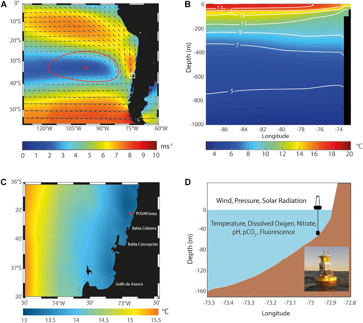
Figure 1. (A) Mean magnitude (ms–1, colors) and direction (vectors) of 10-m winds in the Southeast Pacific during two consecutive summer seasons (2016–17 and 2017–18 years) from ERA5 reanalysis. The red contour and H represent the high-pressure Southeast Pacific Anticyclone (1020 hPa). The box indicates the region where the buoy POSAR is located. (B) cross-section of ocean temperature during November to April from the WOCE/Argo Global Hydrographic Climatology (WAGHC). (C) Sea surface temperature in the study area (°C, colors). The red dot indicates the position of the measurements recorded by the buoy POSAR. (D) Scheme (longitude/depth) of the local topography with the location of the buoy marked.
This alternation between strong/relaxed southerly winds results in a succession of active/inactive upwelling events within summer, reflected in changes of the sea surface temperatures (SST), ocean diffusivities, and surface heat fluxes along the coast (Renault et al., 2009, 2012; Aguirre et al., 2014; Ramajo et al., 2020). Although synoptic upwelling variations have been described in other upwelling regions (e.g., Desbiolles et al., 2014; García-Reyes et al., 2014; Capet et al., 2017), the high frequency and sub-seasonal variability of biogeochemical properties driven by synoptic fluctuations of the coastal winds in the southern Humboldt system remains largely unexplored.
The upwelled ESSW is cooler, rich in nutrients but low in dissolved oxygen (DO) and shows high levels of partial pressure of carbon dioxide (pCO2sea) and low pH values (e.g., Silva et al., 2009; Ramajo et al., 2020). Photosynthesis activity, however, can reduce the high and acidity conditions induced by the coastal upwelling (Duarte et al., 2013; Vargas et al., 2016). These opposing mechanisms and the high-frequency swing between upwelling and downwelling favorable winds make the coast of south-central Chilean a complex system where both physical and biological mechanisms are operating simultaneously controlling the seawater biogeochemistry cycles and the air-sea gas exchange.
Only a few numbers of studies have documented the short-term variability of air-sea CO2 fluxes in response to the change of upwelling/downwelling events at EBUS (e.g., Ikawa et al., 2013; Reimer et al., 2013). Across the Chilean upwelling system, previous studies using satellite and shipboard data have shown a release of CO2 toward the atmosphere (Lefèvre et al., 2002; Torres et al., 2011). However, the direction and magnitude of these air-sea fluxes appear opposite between active upwelling (strong outgassing of CO2) and relaxed wind (CO2 uptake) periods (Torres et al., 1999). The increase in CO2 flux toward the atmosphere during upwelling eventsis due to a combination of the high pCO2sea of the upwelled subsurface waters and large wind speeds since the gas transfer velocity is a function of the wind magnitude (Parard et al., 2010).
Besides, several studies across different EBUS have shown that the nearshore productivity is coupled to local upwelling conditions (e.g., Hutchings et al., 1995; Aguilera et al., 2009; Daneri et al., 2012; Du and Peterson, 2014). Both biological productivity and the structure of the planktonic community can change considerably due to day-to-day variability in coastal wind conditions (Daneri et al., 2012). In the HCS, the delayed response of biological productivity to upwelling-favorable winds has been reported (Aguilera et al., 2009; Daneri et al., 2012). This has been explained by the breakdown of stratification caused by surface mixing, as well as vertical and lateral (offshore) advection during the upwelling favorable winds events, allowing reload of inorganic nutrientstothe euphotic zone. In contrast, wind relaxation provides the necessary stability in the water column to generate phytoplankton blooms (Daneri et al., 2000; Du and Peterson, 2014). Nonetheless, phytoplankton production might change in EBUS areas due to the stronger surface mixing and light limitation associated with enhanced wind stress (Bakun et al., 2015). In this context, the timing between active/inactive upwelling events constitutes a key modulator of the high productivity in EBUS (Lasker, 1975; Hutchings et al., 1995). Indeed, the optimal frequency of wind events, as well as wind intensities, determines the water column primary productivity (PP), signaling the existence of an optimum upwelling range that determines if nutrients are able (or not) to reach the photic zone to be used by the phytoplanktonic community (Lasker, 1975; Hutchings et al., 1995; Cury and Roy, 1989; Bakun et al., 2015) or PP is retained or advected to offshore (e.g., Jacob et al., 2018).
To date, the knowledge of the high-frequency variability of the southern Humboldt system has been limited by the lack of in-situ data of physical and biogeochemical properties in the coastal ocean (e.g., Torres et al., 1999; Ramajo et al., 2020). Here, we take advantage of a unique multiyear record of meteorological and oceanographic measurements acquired by POSAR (Spanish acronym for “Plataforma de Observación del Sistema Océano Atmósfera”), an instrumented buoy about 10 km off the coast of south-central Chile (36.4°S), to describe the response of the surface ocean to periods of strong and relaxed southerly winds during two austral summers (2016–2018). Specifically, we describe: (1) the mean diel variations of biogeochemical variables through the examination of the processes that cause the diel changes, and (2) the high-frequency (days-to-weeks) variability of biogeochemical variables and its relationship to strong southerly wind events. Examination of the variability at diurnal and synoptic timescales put them in perspective and shed light on distinct controls of the surface ocean properties. These two tasks provide the first quantitative assessment of the effect of upwelling events on a comprehensive set of variables and the local air-sea fluxes of heat and CO2 in the coastal ocean off south-central Chile. Our analysis also considers the biological response to upwelling but in a limited way since we only have fluorescence measurementsnear the surface as a proxy of chlorophyll-a. Furthermore, the prospects of climate change consistently predict southerly wind strengthening and drying in this region (Garreaud and Falvey, 2009; Aguirre et al., 2019; Oyarzún and Brierley, 2019) emphasizing the need for understanding atmosphere-ocean coupling and its biogeochemical response.
Materials and Methods
Dataset
The data used in this research has been recorded by POSAR, an automated monitoring meteo-oceanographic buoy located close to Coliumo Bay (Chile) about 10 km off the mouth of Itata River (36.4°S–72.9°W) at waters depths of about 50 m (Figures 1C,D). This platform operated from May 2016 until now, but in discontinuous mode due to land-based maintenance (biofouling removal and sensor verification) every 4–6 months. POSAR data is freely available in real-time at the CR21 and CDOM web portals2.
Two consecutive upwelling seasons (austral spring-summer) were analyzed: from November 2016 to April 2017 and from December 2017 to April 2018. Meteorological variables, measured at about 1 m above sea level, include wind speed (m s–1) and wind direction (°: sex agesimal degrees) recorded every 10 min, whereas air temperature (Tair, °C), sea level pressure (SLP), and relative humidity (RH, %) were logged every 30 min. The oceanographic measurements at 1 m depth were recorded hourly and include water temperature (°C, referred hereafter as sea surface temperature, SST), dissolved oxygen (DO, μM), pH, nitrate (NO3–, μM), the partial pressure of carbon dioxide (pCO2sea, μatm), and fluorescence (RFU). Fluorescence is used here as a proxy for the chlorophyll-a (FChl–a). Hourly temperature (°C) was also recorded at 10 m depth. Supplementary Table 1 shows technical details of the sensors/instruments forming POSAR buoy.
Data Analysis
Diel Cycle
To calculate the mean diel cycle of Tair and SST, DO, NO3–, FChl–a, pH, and pCO2sea, hourly anomaly values were calculated by subtracting the average of each day from the original time series. Then, the seasonal mean and standard deviation were calculated for each hour of the day. In the case of the net radiation, the hourly average values were computed and then the mean and standard deviation for each hour of the day were calculated. Likewise, the 10-min values of wind speed and direction were used to calculate zonal (u) and meridional (v) wind components. Using the hourly mean u and v wind components, the mean diel cycles of wind speed and direction were calculated by averaging each hour of the day.
Bulk Parameterization for the Wind Stress and Heat Fluxes
Hourly averages of meteorological variables (u, v, Tair, SLP, and RH) and SST were used to calculate the surface wind stress, the air-sea latent and sensible heat fluxes using the Tropical Ocean Global Atmosphere Coupled Ocean-Atmosphere Response Experiment (TOGA-COARE) bulk flux algorithm (Fairall et al., 1996). This algorithm is based on the parametrization of Lui, Katsaros, and Businger study (LKB, Liu et al., 1979) that shows a good agreement with observations (e.g., Bradley et al., 1991). The air-sea transfer coefficients for momentum and heat fluxes follow the Monin-Obukhov similarity theory of the atmospheric surface layer.
Air–Sea CO2 Flux
An evaluation of the air–sea CO2 fluxes were obtained from the partial pressure of the CO2 at the surface ocean (pCO2sea) applying the standard bulk formula to the hourly data:
where a constant value of 410μatm is used for atmosphere (pCO2air) (Blunden and Arndt, 2019). The solubility coefficient of CO2 in seawater (α) was calculated using SST and salinity data, following the formulation of Weiss (1974). The CO2 gas transfer velocity (k), as a function of the wind magnitude, was estimated following Nightingale et al. (2000)
where W is the wind speed, and Sc is the Schmidt number. Positive values of fCO2 represent outgassing of CO2 toward the atmosphere, while negative values indicate a CO2 uptake by the surface ocean. Finally, the hourly values of fCO2 were averaged to produce a daily mean value of the flux.
Upwelling Events and Compositing Analysis
To characterize active/inactive upwelling events, we used the Upwelling Index (UI, Bakun, 1975) evaluated at an hourly time-scale:
where τa is the alongshore wind stress, ρw is seawater density, and f is the Coriolis parameter. The hourly wind stress, calculated with TOGA-COARE algorithm, was rotated with respect to the angle of the topography of the continental margin at the buoy location (30.7° clockwise from North) to obtain the alongshore wind stress component (τa). We multiplied by 1000 m so that UI represents the Ekman transport in units of m3 s–1 per km of coastline and by −1 so that positive values imply offshore Ekman transport and hence upwelling of deeper waters. Negative UI indicates onshore Ekman transport and downwelling. The hourly UI time series were smoothed using a 24-h moving-average. The same smoothing was applied to the rest of the variables.
In section “High-frequency variability” we examine the time series of UI along with selected physical and biogeochemical variables during both summer seasons. Upwelling events are defined as a sequence of at least 2 days (48 h) with smoothed UI over 80 m3 s–1 km–1. We chose 2 days as the minimum duration because periods of positive UI lasting less than that do not produce a significant response in the surface coastal ocean. On the other hand, the UI distribution exhibits two modes (not shown), one around zero (calm conditions of either sign) and the other around 250 m3 s–1 km–1 (strong equatorward alongshore winds), with relatively low occurrences around 100 m3 s–1 km–1, since UI experiences sharp changes at the onset and demise of upwelling events. Thus, varying the UI threshold from 60 to 150 m3 s–1 km–1 does not alter our selection of events. Although each upwelling event has its own peculiarities (section “A closer look at upwelling events”), we attempt to describe their common features using a compositing analysis. Because the duration of each event is highly variable (from 2 days to 2 weeks) we have refrained from producing a composite of their full lifecycle. Rather, we focus on the changes at their onset (hour 0−, the instant at which UI changes from negative to positive) and demise (hour 0+, the instant at which UI changes from positive to negative) because the most significant changes occur around the times when UI reverse sign (last part of section “A closer look at upwelling events”). The time spanned by the composite around the onset and demise is 84 h. The averaging was done using the variables relative to hour 0, except for the wind and atmospheric pressure.
To describe the broad-scale meteorological conditions during the upwelling events identified with POSAR data, we performed a composite analysis of selected atmospheric fields at the time of maximum wind stress recorded by the buoy. ERA5 reanalysis data (Hersbach et al., 2020) was used to construct anomaly maps of SLP, surface winds, and SST for each event. This was calculated as the departure from the corresponding long-term (1990–2020) monthly means to then being averaged to construct the composite anomalies. The ERA5 data has hourly resolution being available on a regular grid with 0.25 × 0.25°lat-lonspacing.
The full sample of daily air-sea fluxes were segregated according to UI into upwelling days (upw, UI > 80 m3 s–1 km–1 for more than 2 days), no-upwelling days (no-upw, UI > 0 but not included as upwelling event) and downwelling days (down, UI < 0).
Results
The hourly time series of selected physical and biogeochemical surface ocean variables are shown in Figures 2,3, illustrating the full range of variability during the two summer seasons with POSAR measurements. A customary inspection of these time series reveals a minor (but non-negligible) diel cycle superimposed on large and highly coherent synoptic (several days) variations that are described in the next subsections. In contrast, no clear intraseasonal variability (30–60 days) is observed. The annual cycle is not evident either since the series span from late spring to early fall only.
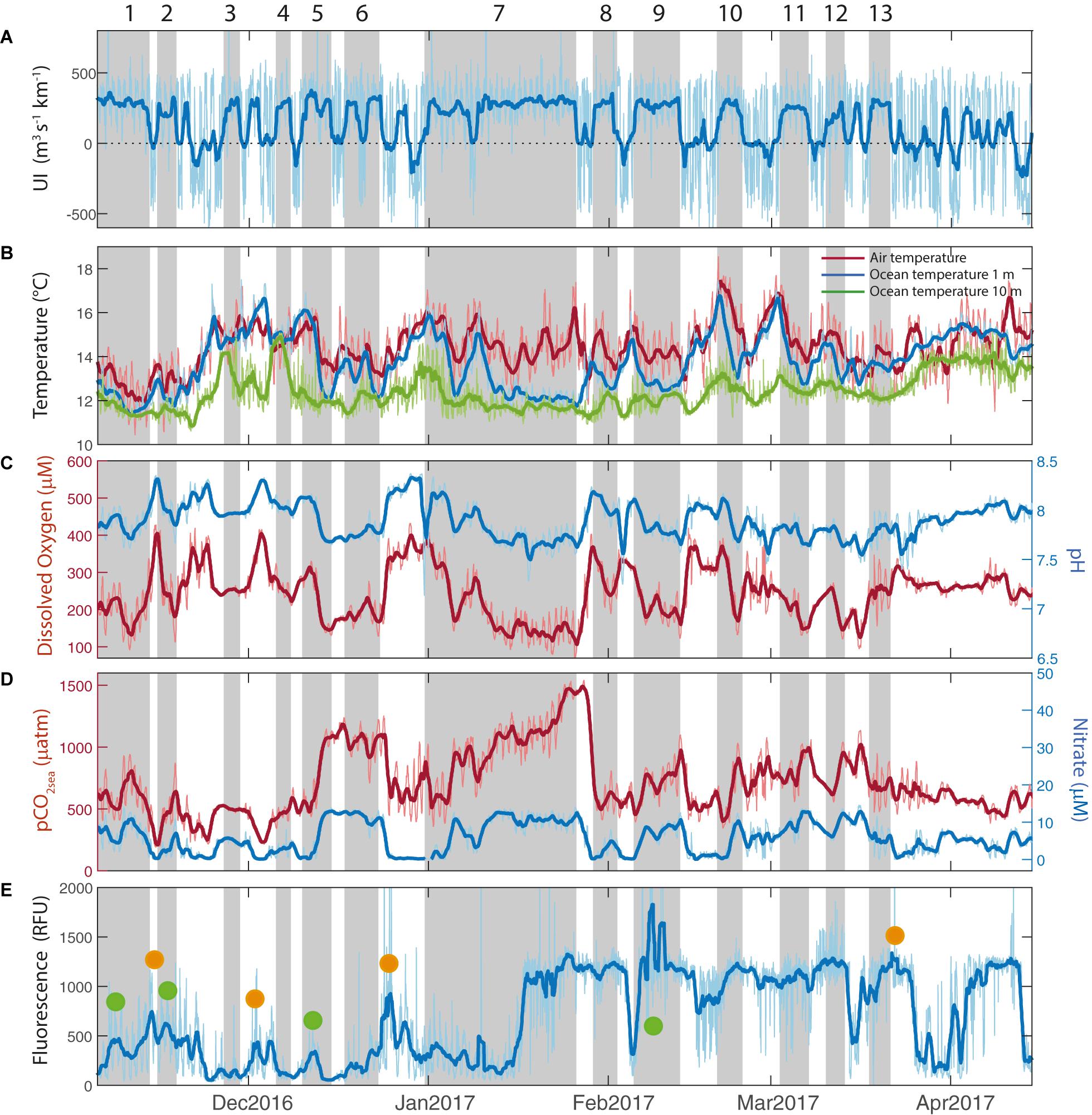
Figure 2. Hourly (thin line) and filtered (thick line) time series between November 2016 and April 2017. Vertical gray bars indicate the periods of the upwelling events. (A) Upwelling Index (m3 s–1 km–1), (B) Air temperature (°C, red line), ocean temperature at 1 m depth (blue line) and ocean temperature at 10 m depth (green line), (C) Dissolved Oxygen (μM, red line) and pH (blue line), (D) pCO2sea (μatm, red line) and Nitrate (μM, blue line) and (E) Fluorescence (RFU). Green dots indicates when fluorescence increases during upwelling events and orange dots indicates when fluorescence increases after upwelling events.
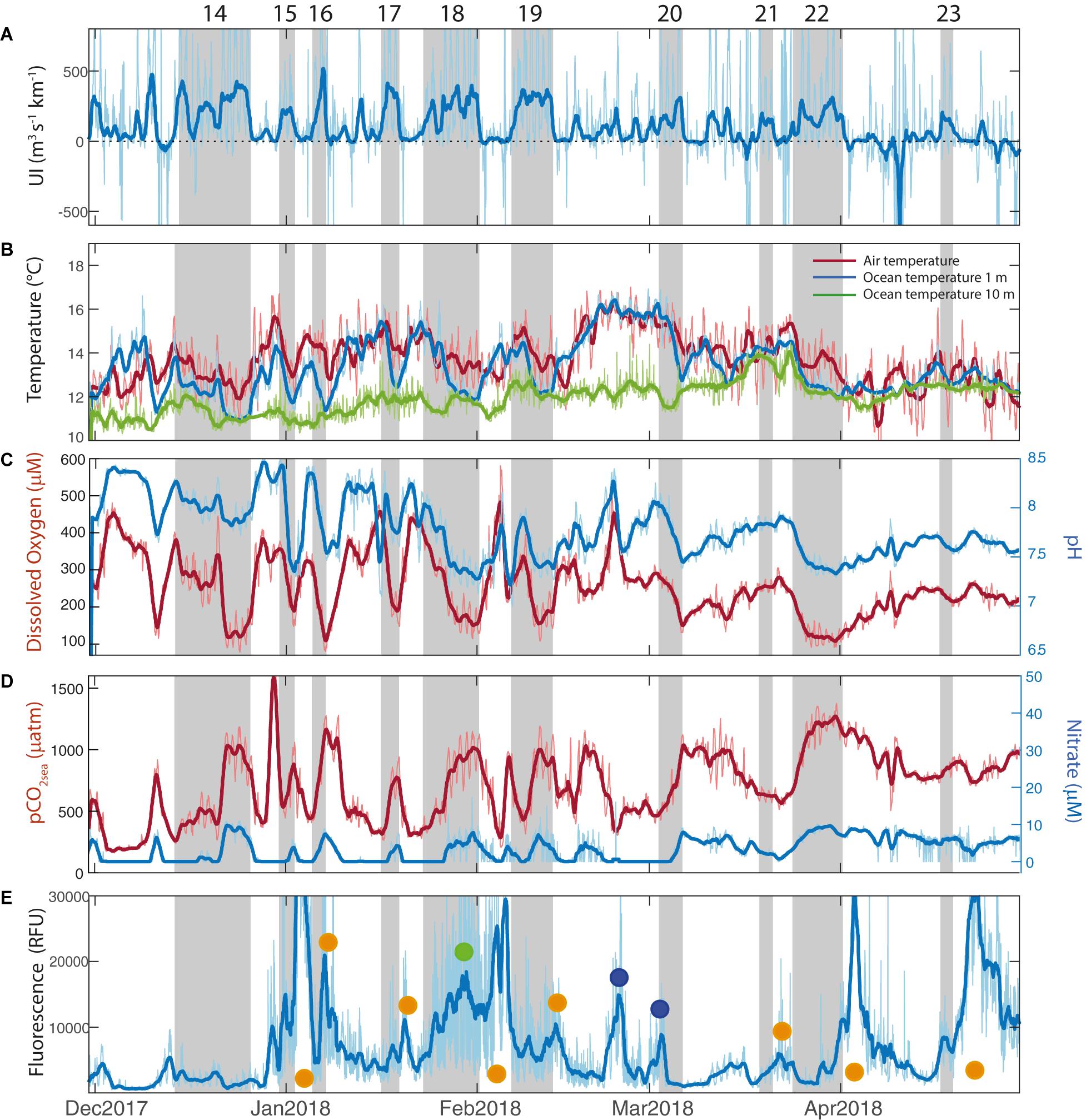
Figure 3. Hourly (thin line) and filtered (thick line) time series between December 2017 and April 2018. Vertical gray bars indicate the periods of the upwelling events. (A) Upwelling Index (m3 s–1 km–1), (B) Air temperature (°C, red line), ocean temperature at 1 m depth (blue line) and ocean temperature at 10 m depth (green line), (C) Dissolved Oxygen (μM, red line) and pH (blue line), (D) pCO2sea (μatm, red line) and Nitrate (μM, blue line), and (E) Fluorescence (RFU). Green dots indicates when fluorescence increases during upwelling events, orange dots indicates when fluorescence increases after upwelling events and blue dots indicates when fluorescence increases decupled from alongshore wind.
Broadly speaking, both summers were comparable in terms of their mean values. In particular, the mean SST was 13.7 ± 1.4°C during summer 2016/2017, slightly higher than the mean SST during summer 2017/2018 (13.3 ± 1.4°C). El Niño – Southern Oscillation (ENSO), the main driver of interannual SST anomalies in central Chile (Montecinos et al., 2003), was in its neutral phase during spring and summer of 2016/2017 and 2017/2018, although Niño 3.4 was slightly negative during these periods and a major coastal El Niño event developed off Peru in January 2017 (e.g., Garreaud, 2018). The minor interannual differences in mean SST seem to be linked to local wind conditions driven by regional-scale anomalies of the SLP (not shown). Indeed, the alongshore wind stress was, on average, more intense during the 2017/18 summer, consistent with lower average values registered for SST and Tair. The accumulated wind stress, however, showed that both periods were similar in terms of offshore Ekman transport (Supplementary Figure 1A).
Mean Diel Cycles
The mean diel cycles of the variables measured at POSAR is presented in Figure 4. To place the diel cycles in context, we compare -for each variable- the diel amplitude (maximum minus minimum values) with the standard deviation computed from the time series of daily mean values. The amplitude of the diel cycle of air temperature was relatively large, about 70% of the day-to-day standard deviation, and the amplitude of the dielwind speed is about a third of the synoptic variability. Consistent with the prevailing clear skies and strong insolation during summer, the amplitude of the solar radiation diel is 5 times larger than the synoptic variability. In general, the amplitude of the daily cycle is smaller for the oceanographic variables. The diel amplitude of SST, DO, and pCO2sea is about 25% of their corresponding standard deviation, and pH, NO3–, and FChl–a have an amplitude of the diel cycle that is about 15% of their standard deviation.
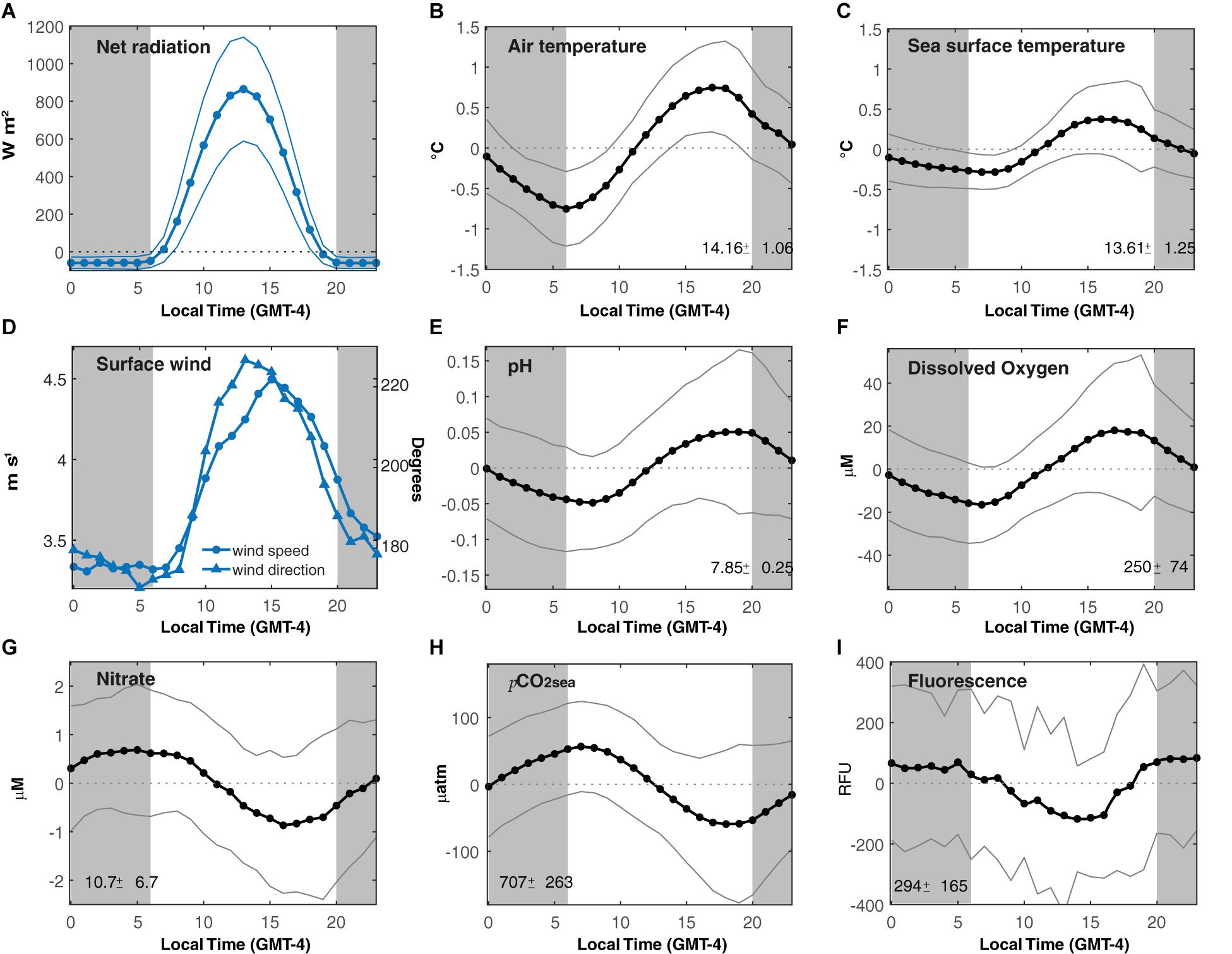
Figure 4. Diel cycle of selected variables measured at buoy POSAR. (A) Net radiation, (B) Air temperature anomalies, (C) Sea surface temperature anomalies, (D) Surface wind speed and direction, (E) pH anomalies, (F) Dissolved oxygen anomalies, (G) Nitrate anomalies, (H) pCO2sea anomalies, and (I) Fluorescence anomalies. Dots represent the mean diel cycle and the thin line correspond to its standard deviation. Vertical gray bars indicate night-time. The mean and standard deviation of daily time series are shown in each panel.
The net radiation (determined by solar radiation, not shown) shows a peak around 13 Local Time (LT) (Figure 4A). The diel cycles of Tair and SST are in phase with maximum values at 16–17(LT) (Figures 4B,C). The mean diel amplitude of the Tair at POSAR is 1°C, about twice larger than the amplitude of SST, but much smaller than the temperature amplitude over land (∼20°C), reflecting a strong thermal inertia of the ocean. In turn, the land-sea thermal contrast controls the diel cycle of the coastal winds. On average, the wind speed increases from less than 3 m s–1 during nighttime to ∼5 m s–1 in the late afternoon. The wind direction is dominated by the southerly component but a westerly (onshore) component develops during the daytime, signaling the effect of the weak land-sea breeze on this near-coastal site (Figure 4D). These results are consistent with the previous characterization of the daily cycle of wind speed and direction in this region using satellite data (Muñoz, 2008).
The surface biological and biogeochemical variables exhibit a clear diel cycle as well (Figure 4). The diel cycle of DO and pH are in phase, with amplitudes of 40 μM and 0.1, respectively. They show a peak during the afternoon (18 LT) and a minimum at dawn (07 LT). Conversely, the diel of NO3– and pCO2sea have maxima before sunrise (07 LT) and minima during the afternoon (16–18 LT) with an amplitude of 2 μM and 100 μatm, respectively. The mean diel cycle of FChl–a increased gradually during daytime reaching maximum values at 21 LT and minima values at 10 LT, with a diel cycle amplitude of 200 RFU. In “Discussion” section, we interpret these diel cycles as a combination of physical and biological processes.
High-Frequency Variability
Within both summer periods, the time series of UI (Figures 2A,3A) reflect the variable wind conditions in the near-coastal zone at the synoptic time scale. Although the seasonal mean condition was favorable to coastal upwelling (UI > 0), a continuous alternation between strong southerlies and weak northerlies (UI < 0, downwelling favorable) is evident. Recall that upwelling events are defined as a sequence of two or more days with UI > 80 m3 s–1 km–1 (section “Upwelling events and compositing analysis”). These events are highlighted in Figures 2, 3 by vertical bars and numbered for further reference. We found a total of 23 upwelling events, 13 during the summer 2016–2017 and 10 during summer 2017–2018 (see Supplementary Table 2 with specific dates in Supplementary Material). During these events the wind speed reaches its highest values and henceocean mixing (function of the cube of wind speed) is enhanced.
The average duration of the upwelling events was 6 days for both study periods with a standard deviation of 3.5 days. Most of the events lasted between 2 and 6 days but, remarkably, one of them extended from 10 to 25 January 2017 (Figure 2A), resulting in high accumulation of wind stress (Supplementary Figure 1B). This period was characterized by abnormally persistent anticyclonic conditions over south-central Chile that brought record high temperature inland along with major forest fires (Bowman et al., 2019). The rest of the summer 2016–2017 was characterized by short-lived (2–3 days) upwelling periods interrupted by even shorter periods of relaxed southerlies or weak northerlies. By the contrary, the summer 2017–2018 had upwelling events more evenly distributed and alternated with relaxed southerlies lasting from 1 to 7 days (Supplementary Table 2). Altogether, the average duration of the inactive upwelling periods was 4.5 days with a standard deviation of 4.2 days. In these periods the wind relaxes to near calm conditions and the mixing is minimum.
Upwelling events were associated with high levels of incoming solar radiation (not shown) and cooler waters at the surface (Figures 2B,3B). In both summers, maximum values of SST up to 17°C occurred during periods of relaxed southerly winds, whereas values as low as 12°C was observed during periods of strong southerlies. The ocean temperature time series registered at 1 and 10 m depth show a clear difference in variability: the SST responds rapidly to changes in UI but the temperature at 10 m depth is less affected. Regardless of the upwelling duration, SST drops 0.7 ± 0.4°C from the beginning to the end of the events. Tair also decreases during upwelling events but less markedly than SST.
The sub-seasonal variability of the near-surface biogeochemical variables is dominated by synoptic-scale changes and modulated by the recurring active upwelling and relaxed periods. The first column in Table 1 shows the maximum correlation between UI and the different biogeochemical properties, along with the time lag that maximizes their association. Results show that coastal SST and UI are negatively correlated, and the correlation maximizes with lags of 1.5 days, which is consistent with previous studies in this region using in-situ and remote sensing SST and wind data (Renault et al., 2009; Aguirre et al., 2014). The UI shows negative correlations with DO and pH which are maximized at lags between 1 and 1.5 days. pCO2sea and NO3– are positively correlated with maximum values at lags of ∼30 h and ∼20 h, respectively. By the contrary, insignificant correlations are found between UI and FChl–a. Table 1 also shows the correlation coefficients among biogeochemical variables. Most of the correlations are significant and similar between both summers, indicative that the wind-driven control results in highly coherent variations among the biogeochemical properties, except for the case of FChl–a.
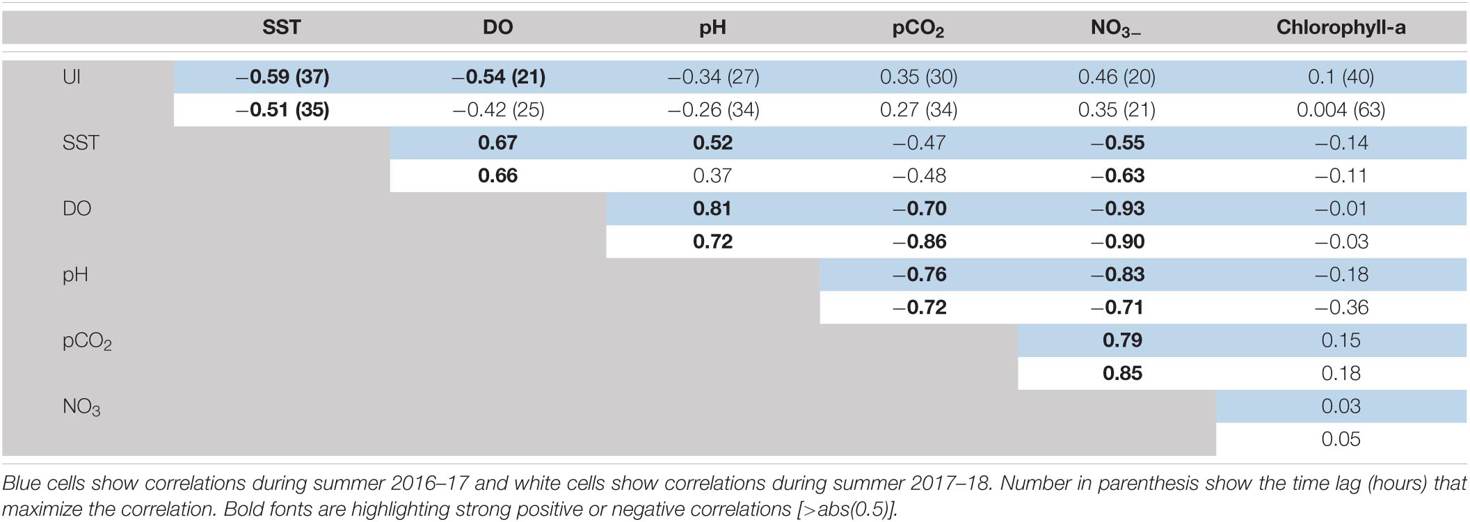
Table 1. Spearman coefficient correlations of sea surface parameters collected at POSAR buoy off central Chile.
The time series of DO show a wide range of variation with maxima up to 400 μM in relaxed events and minima about 100 μM during active upwelling events, particularly those when positive UI persists for long periods (Figures 2C, 3C). The pH shows relatively low values during active upwelling events, and higher values during relaxed winds periods (Figures 2C, 3C). pH also shows a positive correlation with DO (0.75, p < 0.05) (see Table 1). In the same way, preformed NO3– is never depleted in the surface water with a lower threshold level of about 3 μM but increases up to 20 μM during active upwelling events (Figures 2D, 3D). NO3– concentrations decreases during southerly wind relaxations, particularly in those when negative UI persists for more than 3 days.
NO3– exhibits a high and significant negative correlation with DO and pH. pCO2sea shows a similar pattern to the other biogeochemical variables, rapidly increasing during upwelling events. It reached values as high as 1500 μatm during the protracted upwelling event in January 2017. pCO2sea is negatively correlated with DO and pH, and positively correlated with NO3– concentration (see Table 1).
The FChl–a time series show a complex variability that not always follow the variation of other physical and biogeochemical variables during active and relaxed upwelling events (Figures 2E, 3E). Indeed, FChl–a has insignificant correlations with UI, oceanographic and biogeochemical series (Table 1). During the summer 2016–2017 FChl–a remained low (100–500 RFU) from November until mid-January. During the long upwelling event, FChl–a had a sharp and substantial increase and remained high (∼1200 RFU) until the end of March 2017. During this summer season there were short-lived excursions of FChl–a not obviously related to active upwelling events. In the summer of 2017–2018, FChl–a exhibited more variability at the synoptic time scale in the form of large spikes of 2–4-day duration. Considering both summers, 12 (out of 23) upwelling events have a substantial increase of FChl–a after the event demise (i.e., under relaxed winds). On the other hand, 10 spikes of FChl–a were not obviously related to wind changes (Figures 2E,3E). These large variety of FChla–a responses (or the lack of) to upwelling events suggest a complex control of physical and biological conditions as discussed in section “Biogeochemical response”.
A Closer Look at Upwelling Events
In describing the high-frequency variability of physical and biogeochemical variables during the two summers with POSAR data (Figures 2, 3) we have broadly documented the impacts of southerly wind events in the surface ocean. A closer look at these events is presented next. Figure 5 includes the evolution of the POSAR variables during a week of strong southerlies that began on March 25, 2018 (event number 22) and that is followed by a several days with relaxed winds. A drop of temperature of about 2°C occurred at both 1 and 10 m depth within the first 72 h of the event, followed by a much weaker cooling until its end. After that, there is a surface (1 m) warming of ∼0.5°C in the first 2 days with relaxed winds. The air temperature tends to follow the ocean temperature but with an attenuated amplitude and additional short-term variability. Also evident during the event is the decrease in DO (−100 μM) and pH (−0.4) as well as the increase in pCO2sea (+800 μatm) and nitrate (+5 μM). Although these variables were not steady before the onset of the strong southerlies, but the largest changes occurred in the first 3 days (4 days in the case of pCO2sea) of the upwelling followed by weaker trends until the end of the event when their evolution is reversed.
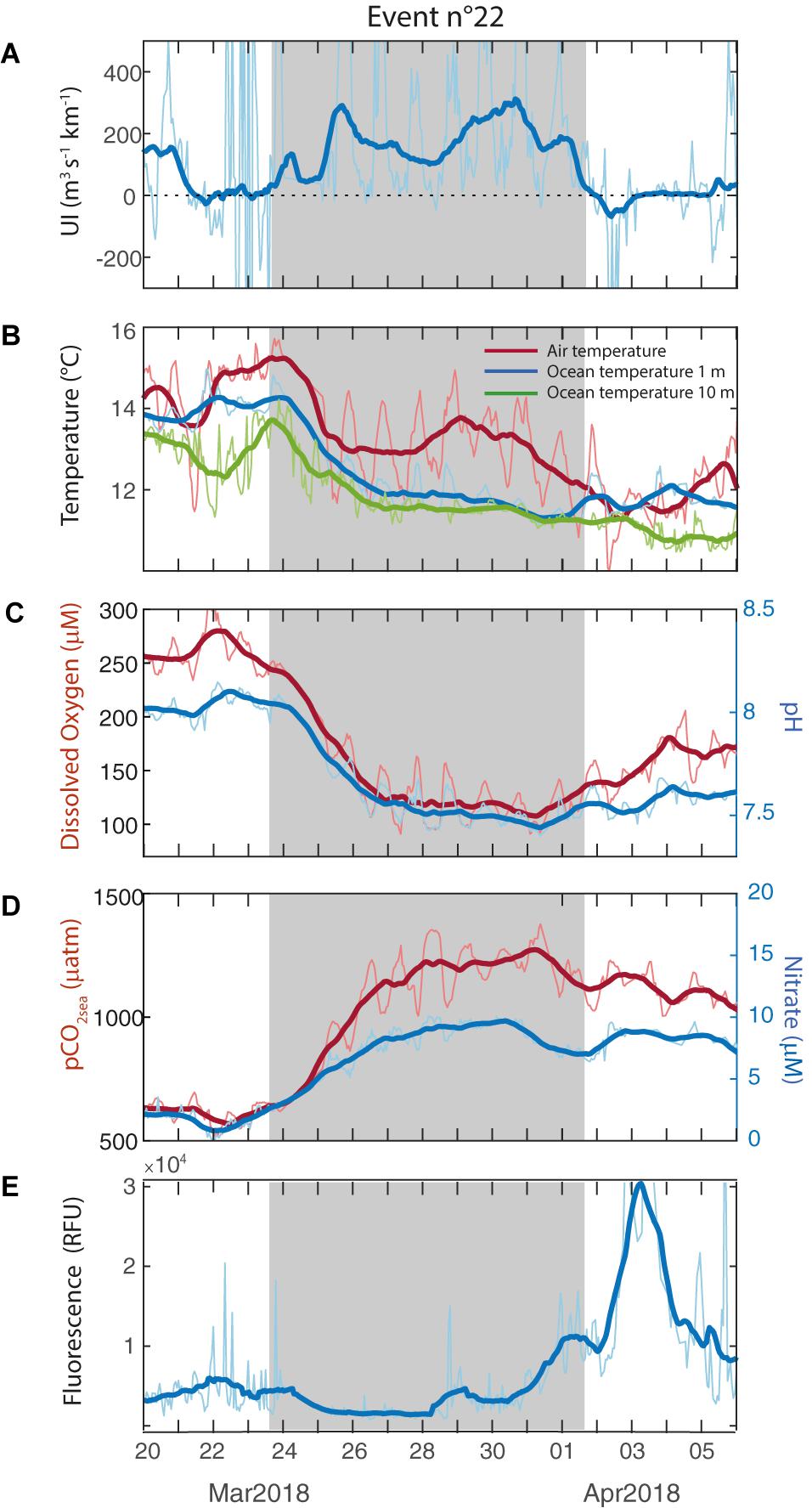
Figure 5. Close-up to a strong upwelling event that began on March 25, 2018 (event number 22) followed by relaxed alongshore winds. (A) Upwelling Index, (B) Air temperature (°C, red line), ocean temperature at 1 m depth (blue line) and ocean temperature at 10 m depth (green line), (D) pCO2sea (μatm, red line) and Nitrate (μM, blue line), (C) Dissolved Oxygen (μM, red line) and pH (blue line) and (E) Fluorescence (RFU).
The fluorescence was low during the first half of the strong southerly wind period, followed by gradual increase over the last 3 days (Figure 5D). However, the most important rise (∼10 times the initial values) occurred during the subsequent relaxed period, about 2 days after the upwelling demise. To illustrate the variety of fluorescence responses, Figure 6 depicts another upwelling event (number 20). Despite the shorter duration of the strong southerlies, SST, DO, pH, pCO2sea and NO3– show a response similar to the event 22. By the contrary, there was a peak in FChl–a at the beginning of the event followed by persistent low values (Figure 6D).
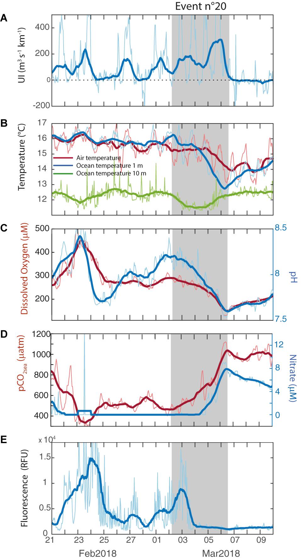
Figure 6. Close-up to an upwelling event that began on March 02, 2018 (event number 20). (A) Upwelling Index, (B) Air temperature (°C, red line), ocean temperature at 1 m depth (blue line) and ocean temperature at 10 m depth (green line), (D) pCO2sea (μatm, red line) and Nitrate (μM, blue line), (C) Dissolved Oxygen (μM, red line) and pH (blue line) and (E) Fluorescence (RFU).
To further describe the response of physical and biogeochemical ocean variables to wind changes a compositing analysis is now presented. Given their variable duration, we have refrained to produce a single composite for the full upwelling events but, instead, we performed separated composites based on their onset and demise (see section “Upwelling events and compositing analysis” for details).
The alongshore winds are near 0 or slightly from the north (downwelling favorable) before the onset of the events (hour 0- when UI changes from negative to positive) and they increase rapidly in the next 12 h. By the contrary, the cross-shore winds exhibit little changes during the onset of upwelling events. After the ramp-up period the wind speed is relatively constant at ∼5 m s–1 (Figures 7A,B) about twice stronger than in periods outside the events. The SLP increases by about 2 hPa from 1 day before to 1 day after the onset (Figure 7C), signaling the establishment of anticyclonic conditions during the early stage of upwelling period.
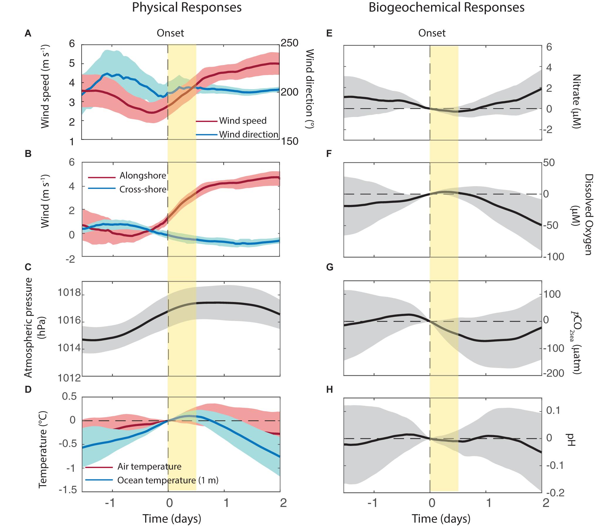
Figure 7. Composite analysis of selected variables during the onset of the upwelling events. (A) Wind speed and direction, (B) Alongshore wind (red line) and cross-shore wind (blue line), (C) Sea level atmospheric pressure, (D) Air temperature (red line) and ocean temperature at 1 m depth (blue line), (E) Nitrate, (F) Dissolved Oxygen, (G) pCO2sea and (H) pH. Vertical yellow bars indicate 12 h after the onset of the upwelling events.
The ocean temperature at 1 m (SST) begins to react about 12 h after the event onset decreasing linearly about 1°C in the following 36 h. The near-surface air temperature (Tair) also tends to decrease during the initial stage of the upwelling events, but with a smaller amplitude (about 0.3°C on average) and a lag of about 12 h in comparison with SST evolution (Figure 7D). Nearly synchronous with SST, DO begins to decrease about 12 h after the onset reaching an anomaly of −50 μM (relative to time 0) 2 days after the upwelling event onset. The NO3– concentration has a more delayed response, as it remains nearly constant during the first 24 h of an upwelling event, but it later showed, on average, an increase of 2 μM in a day (Figures 7E,F). Notably, pCO2sea begins to decrease as soon as the upwelling event begin, reducing its value by about 100 μatm 1 day later, but then rises as the upwelling event develops. pH values remain unchanged the first 1.5 days, and slightly decreases in 0.05 units 2 days after the onset of the upwelling event (Figures 7G,H).
Considering the demise of the upwelling events (Figure 8), our compositing analysis shows that the deceleration of the alongshore winds is concentrated in the 12 h prior to the demise (hour 0+ when UI changes from positive to negative) followed by a period of calm or weak northerlies (Figures 8A,B). The SLP exhibits a minimum close to time of the demise (Figure 8C), in connection with the arrival of a coastal low to the POSAR area as described in section “Synoptic-scale conditions”. SST often reaches a minimum about 1 day before the event’s demise. It begins to rise about 0.5°C during the last 12 h of the upwelling event and another 0.5°C in the next day under relaxed wind conditions (Figure 8D). NO3– exhibits a maximum 1 day before the demise and then begin to decrease in synchrony with UI, producing an overall drop of about 6 μM within 48 h from the end of the upwelling event to the beginning of the relaxed wind period (Figure 8E). The behavior of the DO and pH is nearly the specular image of the NO3– evolution, with an increase that begin about 12 h before the upwelling demise and continue during the next 36 h (Figures 8F,G). As expected, the pCO2sea and pH in the surface layer also show a similar but opposite evolution when the event demise, indicative of the reliability of the POSAR measurements. pCO2sea (pH) keeps increasing (decreasing) until the demise of the upwelling event thus reaching its maximum (minimum) close to hour 0+. After that, pCO2sea decreased by 100 μatm and pH increases by 0.15 units in about 1 day under calm conditions (Figures 8G,H).
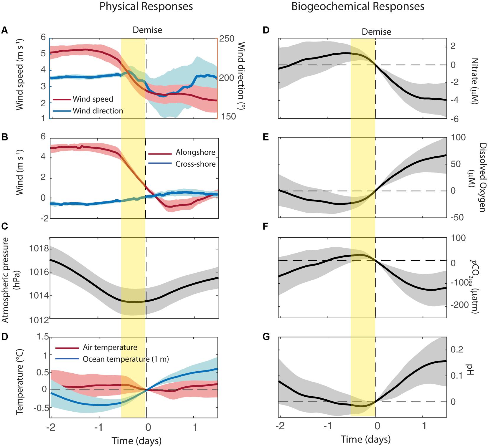
Figure 8. Composite analysis of selected variables during the demise of the upwelling events. (A) Wind speed and direction, (B) Alongshore wind (red line) and cross-shore wind (blue line), (C) Sea level atmospheric pressure, (D) Air temperature (red line) and ocean temperature at 1 m depth (blue line), (E) Nitrate, (F) Dissolved Oxygen, (G) pCO2sea, and (H) pH. Vertical yellow bars indicate 12 h before the demise of the upwelling events.
Air-Sea Heat and CO2 Fluxes
In closing this section, we estimate the magnitude of the heat (latent and sensible) and CO2 fluxes in the near-coastal zone off south-central Chile and explore how they vary between periods of strong and weak southerly winds. The bulk formulas employed in the calculations of air-sea fluxes were presented in section “Data analysis” to produce daily mean values. The full sample was then divided among upwelling days, transition days, downwelling days, and the last day of each upwelling event (section “Upwelling events and compositing analysis”). The box plots synthetizing the distribution of the heat fluxes in each subsample are presented in Figure 9. As expected for an upwelling region the summer mean SST was 0.5°C lower than Tair. Consistently, the summer-median sensible heat flux is from the air to the ocean (negative) but small, about −5.4 W m–2 and with a large interquartile range (0.4 to −10.1 W m–2) due to the swings between active/inactive upwelling periods. The median sensible heat flux during upwelling days reached −7.4 W m–2, but close to zero or even from the ocean to the air (positive) during transition and downwelling days. On the contrary, the summer median latent heat flux was +9.4 W m–2, as the air above the water was typically sub-saturated and the slightly warmer air temperature is not able to increase the mixing ratio above the surface saturated value. Considering upwelling days, the latent heat flux was even larger, with a median of 12.5 W m–2 and an upper quartile of 25.1 W m–2, due to the increased surface wind speed.
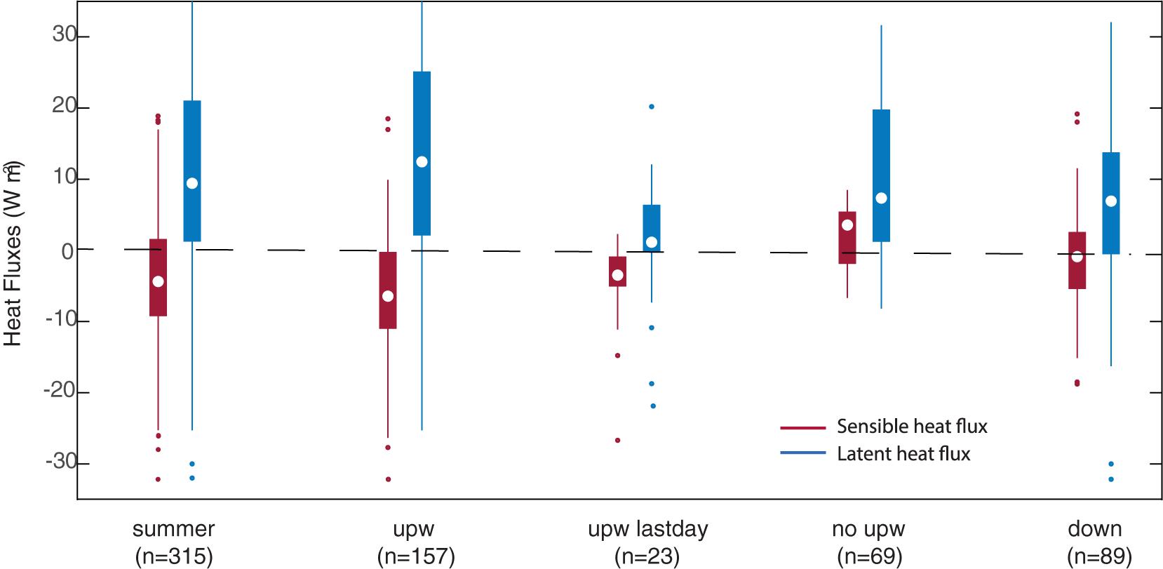
Figure 9. Box plot of the daily mean sensible (red) and latent (blue) heat flux of the full sample (summer), the upwelling days (upw), the last days of the upwelling event (upwlastday), the no-upwelling days (no upw) and downwelling days (down). Circle indicates median, boxes the range 25th and 75th percentiles, lines extend to the most extreme data and dots are outliers.
The summer median CO2 flux at POSAR was +10.4 mmol CO2 m–2 d–1 with an interquartile range of 4.1 and 22.9 mmol CO2 m–2 d–1 (Figure 10). We found that about 75% of the total outgassing occurred in the 157 days of upwelling that represent 50% of both summer seasons. During upwelling events, the median flux was 12.1 mmol CO2 m–2 d–1, but the distribution included values as large as 51 mmol CO2 m–2d–1. During downwelling events, as well as transition days, the flux of CO2 decreased, but even then, more than 75% of the time the coastal ocean was releasing CO2 to the atmosphere.
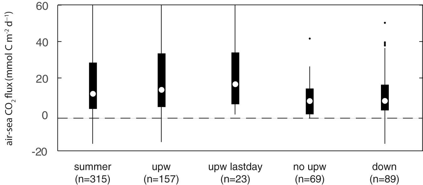
Figure 10. Box plot of the daily mean air-sea CO2 flux of the full sample (summer), the upwelling days (upw), the last days of the upwelling event (upwlastday), the no-upwelling days (no upw) and downwelling days (down). Circle indicates median, boxes the range 25th and 75th percentiles, lines extend to the most extreme data and dots are outliers.
Discussion
Synoptic-Scale Conditions
To place the active upwelling events detected at POSAR on a broader scale meteorological setting we performed a composite analysis of SLP, surface winds and SST fields 24 h before the event demise (referred to as tmax), approximately the time of maximum southerly wind and minimum SST over the coastal ocean (see Figure 8). The average anomalies maps considering the 23 events identified in both summer periods are shown in Figure 11. Examination of individual maps revealed a high degree of coherence among them lending support to the use of the composite maps. The SLP field at the time of maximum alongshore wind stress at POSAR (Figure 11A) shows the SPA centered at its climatological position during summer (about 35°S, 85°S) and with normal strength (∼1025 hPa) but bulging toward the southern coast of South America in connection with a migratory high-pressure cell that has moved from the South Pacific Ocean toward the continent in the last few days (Aguirre et al., 2021). This evolution is consistent with the gradual increase in SLP recorded by POSAR in the early stages of the upwelling events (e.g., Figure 7C). By tmax, the migratory high-pressure system was already over Argentina, as revealed by the positive SLP anomalies to the east of the Andes, although its rear side is still over southern Chile producing a pressure increment of about 3 hPa over the coastal region to the south of 39°S. Farther north there is a trough along the coast, which is a common feature during summer months (Muñoz, 2008). Nevertheless, the coastal trough has deepened -up to 2 hPa- between 35 and 25°S revealing the mature stage of a coastal low, a sub-synoptic system that develops in connection with the migratory anticyclone farther south (Garreaud et al., 2002).
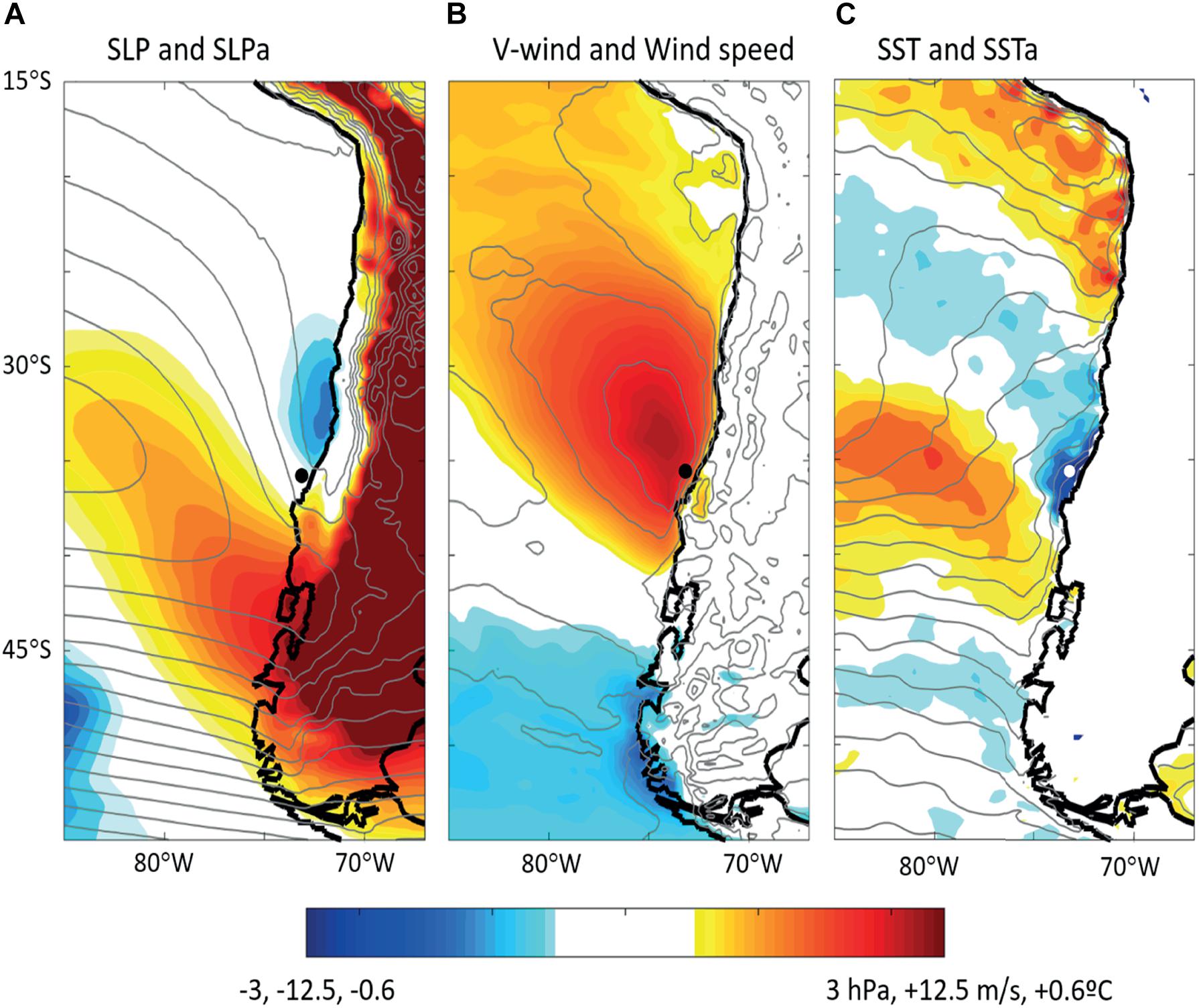
Figure 11. Composite maps 24 h before the upwelling events demise constructed using ERA5 reanalysis data. (A) Sea level pressure (contours) and sea level pressure anomalies (colors), (B) Meridional wind (contours) and wind speed (colors), (C) Sea surface temperature (contours) and sea surface temperature anomalies.
Within this synoptic context, the POSAR buoy is located just in between the positive SLP anomalies to the south and the negative anomalies to the north that steepen the meridional pressure gradient at 38–36°S. The presence of the coastal range breaks down the geostrophic balance at low levels thus resulting in intense alongshore flow (Garreaud and Muñoz, 2005), consistent with the strong upwelling favorable winds recorded by our study around tmax (Figures 7B, 8B). Indeed, the composite map of 10-m meridional wind and wind speed (Figure 11B) shows a broad area of southerly winds greater than 10 m s–1 off central Chile with its core encompassing the POSAR site. The largest wind speed is farther offshore, but the near-shore winds do cause the coastal upwelling cooling the ocean surface between 30 and 38°S (Figure 11C). The later composite must be taken with caution as it comes from reanalysis data, however, the magnitude of the average cooling (∼−0.5°C) is within the range of the POSAR values during the next days of the onset of the upwelling events (Figure 7D). Further, a one-point correlation analysis between the meridional wind stress and SST confirms the composite results (Supplementary Figure 2).
Physical Response
Several studies in EBUS provide examples of SST variability associated with the alternation between upwelling- and downwelling-favorable winds periods, including the Humboldt system (e.g., Renault et al., 2009, 2012). Our findings show that SST responds rapidly (∼12 h) to changes in alongshore wind direction, but the temperature at 10 m depth is mostly unaffected, a pattern consistent with a pronounced but shallow thermocline. In the same region and comparable water depth, the mean summer thermocline has been previously observed at 3–7 m depth (Aguirre et al., 2010). Thus, the inner shelf water column becomes more mixed during active upwelling events and more stratified during relaxed winds periods as observed in other coastal upwelling systems (e.g., Lentz, 1992).
An estimate of the contribution of the vertical advection to the surface ocean cooling during an upwelling event can be obtained by calculating Ekman vertical velocities and vertical temperature gradient at 10 m and 1 m depths. Using such approximation, it was found that the vertical advection (about −0.3°C d–1) represents roughly half of the total heat loss during the first day of the upwelling event. Although the Ekman vertical velocity continues to increase, following the alongshore winds, its effect decreases as the event develops because the vertical temperature gradient weakens. Overall, the latent heat flux during upwelling periods tends to cool the ocean, but when it is distributed in a 5 m water column results in a cooling rate of –0.05°C d–1 which is close to the estimations made by Renault et al. (2009) and one order of magnitude less than observed cooling. Furthermore, toward the end of the upwelling period, the latent heat flux decreased and even became positive in the upper quartile. Latent heat flux toward the ocean is generated when the SST decrease produces a saturation mixing ratio at the surface that can be lower than the mixing ratio of the air above the interface (Beardsley et al., 1998). Additionally, sensible and latent heat fluxes at the surface tend to compensate each other, and higher amounts of solar radiation reach the surface since clouds tend to dissipate during southerly jet events (Garreaud and Muñoz, 2005), emphasizing the much crucial role of the vertical advection and mixing in cooling the surface ocean during the upwelling events.
Our results are consistent with a modeling study of the coastal ocean heat budget during an atmospheric low-level jet off central Chile (Renault et al., 2012). The authors showed that inside the nearshore zone, the ocean surface cooling during an upwelling event is mainly driven by a combination of vertical advection of upwelled waters and vertical mixing, where each one corresponds to approximately half of the total heat loss. Due to the cooling increases the density of surface waters, it produces more unstable conditions that combined with the increased wind intensity can generate strong vertical mixing. However, there are some limitations associated with the calculation of the heat budget using our data set. For example, the choose of an upwelling length scale to estimate the vertical velocities associated with Ekman transport, and uncertainties in the coastal wind drop-off to estimate the contribution of the Ekman suction (pumping) to vertical velocities. Indeed, this illustrates the complexity of the upwelling mechanisms in this region, as well as the need for a three-dimensional picture to close the heat budget.
Until now we have focus on the response of the surface ocean to the strong forcing induced by the high-frequency variability of the wind. The physical properties in the POSAR region can also be influenced by intraseasonal variability (40–60 days) associated with coastal trapped waves traveling poleward along the continental shelf. These waves are ultimately forced by winds along the equator, and can influence coastal circulation, exchange, and mixing (Huthnance, 1995). The wave-related deepening and rising of the thermocline (pycnocline) is on the order of tens of meters (Leth and Middleton, 2006; Belmadani et al., 2012) and could impact in the response of the SST to upwelling events off central Chile (Hormazabal et al., 2001). However, the length of time series at POSAR (∼5 months each summer) are insufficient to reliably isolate and quantify the impact of remote forced coastal trapped waves in the SST response to the strong synoptic variability of local alongshore winds.
Biogeochemical Response
We begin this discussion by considering the diel cycle of biogeochemical variables. The increase of southerly winds from morning to late afternoon should enhance the upwelling of oxygen-poor, high pCO2sea, low pH, and nutrient rich waters. The observed diel cycles (Figure 4), however, are opposite to these expectations, suggesting an important biological control (e.g., grazing, predation) as it has been observed in other upwelling systems (e.g., Thompson et al., 2012; Kapsenberg and Hofmann, 2016). Other factors such as changes in the horizontal water mass movement are also determinants to define biogeochemical signals across the water column (Neveux et al., 2003; Frieder et al., 2012). Changes in gas solubility for CO2 and DO because of variations in water temperature (Sarmiento and Gruber, 2006) can be excluded as the diel cycle of SST is not in phase with the diel cycle of gas content. Thus, the diel variability of gas content in the surface seems to respond to biological cycles of organic matter respiration and mineralization.
During daylight, phytoplankton biomass is synthesized by photosynthetic activity, where DO is produced and CO2 is assimilated, controlling pH (increase), and consuming NO3– (decrease). In contrast, respiration dominates during night, consuming DO and producing CO2, thus decreasing pH and increasing NO3-. At the continental shelf where the POSAR buoy is located, fluorescence maximum occurs in late afternoon (Figure 4I), contrary to classical studies that reported maxima at midday or early afternoon, as the photosynthetic capacity and its associated carbon fixation to follow circadian solar radiation (Sournia, 1975; Suzuki and Johnson, 2001). These observed net changes could be related to a periodicity of zooplankton feeding on phytoplankton, as early suggested by Mc Allister (1963) or even due to the strong photoinhibition occurring during summertime when solar radiation exceeds 1000 W m–2 around midday. Our high-resolution data (hourly) shed light on phytoplanktonic dynamics, that seems to experience a tradeoff between light (supplied by solar irradiance from the surface water) and nutrients (supplied by upwelling; Mellard et al., 2011), and the maxima fluorescence can be coinciding with the nutricline and not necessary on the surface. Furthermore, diel fluorescence variations could be associated not only with changes in the chlorophyll cell content (Owens et al., 1980), but also a delayed response of the phytoplankton population growth with nutrients availability in the same area (Masotti et al., 2018).
Beyond the diel cycle, POSAR data shows intense sub-seasonal, high-frequency biogeochemical fluctuations largely forced by shifts in the magnitude of the along-shore winds. During periods of strong southerlies, DO and pH decrease and NO3–, air-sea fluxes of heat, and pCO2sea increase; the opposite behavior was found during periods of relaxed southerlies. The decreasing DO conditions during upwelling events respond to the advection of oxygen-poor subsurface water associated with the ESSW. Although the surface layer is usually oxygenated, values near 100 μM at 1 m depth were observed, representing a clear DO deficit, which intensifies as water depth increases becoming hypoxic or even anoxic near the bottom (Farías et al., 2015; Ramajo et al., 2020). Massive fish death along central Chile have been related to such anoxic conditions near the area where POSAR is located (Hernández-Miranda et al., 2012) although such ecological events were not reported during the summers with POSAR measurements. Also, increasing scallops mortalities have been observed under low oxygen conditions driven by upwelling in the northern Chilean coast (Ramajo et al., 2020). Finally, pCO2sea and pH variability agree with the properties of remineralized upwelled waters which present low pH and high CO2 concentrations (Schulz et al., 2019; Ramajo et al., 2020).
Most of the time the CO2 content in surface water was supersaturated with respect to the atmospheric concentration resulting in outgassing. By keeping constant pCO2sea or wind speed in the standard bulk formula (1) we infer that day-to-day variations in the CO2 partial pressure were the leading factor in controlling the changes in CO2 fluxes. It has been observed that such maximum coastal surface water pCO2sea set up a robust cross-shore pCO2sea gradient during active upwelling events off central and northern Chile (e.g., Torres et al., 1999, 2002) as well as in other coastal upwelling systems (e.g., Feely et al., 2008). These results are consistent with previous research at the Peruvian coast, the northern upwelling system of Humboldt, where observational and modeling studies have shown a significant CO2 flux from the ocean to the atmosphere (Copin-Montégut and Raimbault, 1994; Friederich et al., 2008; Mongollón and Calil, 2018). There, a strip about 300 km from the coast is an important source of CO2 toward the atmosphere, and through a series of model experiments, it has been shown that the high pCO2sea is primarily the result of coastal upwelling, which is incompletely compensated by biological activity (Mongollón and Calil, 2018). Along the coast of Chile, air-sea CO2 fluxes have been measured from several expeditions showing the direction of the carbon flux changes from CO2 outgassing at the coastal upwelling region, consistent with our results, to CO2 sequestering at the non-upwelling fjord region in Chilean Patagonia (Torres et al., 2011).
Primary productivity is related to the high-frequency variability introduced by the relaxed and strong wind periods (e.g., Aguilera et al., 2009; Daneri et al., 2012; Du and Peterson, 2014; Hutchings et al., 1995). During upwelling events there is a continuous injection of nutrients into the photic layer. However, intense mixing in the surface layer due to the strong winds can avoid the development of phytoplankton in these periods (Du and Peterson, 2014). Thus, an optimal window for phytoplankton bloom is expected a few days after the southerly winds relax (e.g., Rykaczewski and Checkley, 2008; Ramajo et al., 2020). In the same region of POSAR (but farther offshore) previous in-situ measurements reveal the occurrence of events when primary productivity rates were extremely high with peaks as high as 18.2 g C m–2 d–1, but they do not occur with high wind stress or with colder water (Testa et al., 2018), since chlorophyll-a accumulation requires an optimal window of reduced winds (Wilkerson et al., 2006; Bakun et al., 2015). Over a 5- to 10-day time scale this active-relaxing cycle produces the accumulation of biomass, increases PP rates, and changes microbial community composition (Rutllant and Montecinos, 2002). Considering the two summers with POSAR data we found that just over 50% of the upwelling events lead to a phytoplankton blooms.
Clearly, the above-described wind-phytoplankton biomass association does not hold in a sizeable number of cases. The lack of phytoplankton blooms after active upwelling periods was already observed by Jacob et al. (2018) in the study area and attributed to a combination stratification driving mixing and turbulence processes of different magnitude, and offshore transport of nutrients and productivity (Renault et al., 2012; Astudillo et al., 2019). In addition of the physical condition of the system not reaching its optimal window, other factors (biological) such as changes in the phytoplankton community (e.g., Lee et al., 2013), phytoplankton size (e.g., Montecino and Quiroz, 2000; Shin et al., 2017), food-web dynamics (e.g., Armengol et al., 2019), or biota consumption (Thompson et al., 2012) could be also responsible for why not all upwelling events generate phytoplankton blooms and the lack of linearity between upwelling and fluorescence observed in POSAR data.
Conclusion
In this work, we have characterized the response of surface physical and biogeochemical properties to the sub-seasonal, high frequency variability of the alongshore wind stress off south-central Chile (36.4°S). We also estimate wind-driven changes of heat and CO2 air-sea fluxes. To this effect, we used meteorological and oceanographic high-resolution (hourly) measurements recorded by POSAR buoy in two consecutive spring-summer seasons (November-April of 2016–2017 and 2017–2018). Some of these changes are in line with expectations for a coastal upwelling region, POSAR data allows robust, quantitative estimates of mean amplitude, variability and timescale of the surface ocean responses. During the study period the region experienced 23 upwelling favorable, strong southerly wind events, lasting from 2 days to 2 weeks, intermixed with weak southerlies or even periods of northerly winds. We show that this alternation between active and inactive upwelling conditions introduce more variability in the surface ocean than the diel cycle driven by insolation and biological processes. The upwelling events in the POSAR region are associated with the establishment of a southerly low-level jet that in turn develops in response to a strong along-shore pressure gradient between a migratory surface anticyclone in southern Chile (40–45°S) and a coastal-low in central Chile (25–35°S). Although each upwelling event has peculiarities and different durations, the physical and biogeochemical responses are highly coherent, as documented here for two cases and synthesized by a compositing analysis of their onset/demise. During upwelling conditions (relaxed periods) variables such as temperature, DO, and pH decrease (increases). In contrast, NO3– and air-sea fluxes of heat and CO2 increase (decrease) during upwelling conditions (relaxed periods). In fact, the study area is a source of CO2 to the atmosphere mainly driven by wind speed due to the surface ocean pCO2sea is supersaturated with regard to the pCO2air. In contrast to other variables, surface chlorophyll-a (as inferred from fluorescence) shows a wider range of response to upwelling and relaxed wind conditions. In line with the idea of an environmental optimal window, we found that most peaks in of FChla–a occurred 1–2 days after the demise of upwelling events (about 60% of the cases), but several peaks occurred decoupled of the wind events revealing the complex interplay between physical and biological forcing of the phytoplankton blooms.
The multi-season, high-resolution and comprehensive set of measurements provided by POSAR have allowed a first attempt to describe the complex response of the surface ocean to variation of upwelling/downwelling off the coast of south-central Chile during austral summer. Although such response is broadly consistent with the vertical advection of ocean properties such as potential temperature, nutrients, DO and pH, the quantitative results presented here serve as a firm basis for future model evaluation and validation of remote-sensed estimates. Complementing POSAR near-surface results with vertical profiling capabilities are expected in the near future to provide a fully three-dimensional view of the coastal processes in this seasonally active upwelling region. The use of observation platforms of the coupled ocean-atmosphere system is of vital importance for the country and the region, especially where outcomes from a coupled physical-biochemical model by Brochier et al. (2013) project decreasing nursery areas for small pelagic fish under climate change in the Humboldt ecosystem, that most likely will bring enhanced southerly winds and drying conditions.
Data Availability Statement
The original contributions presented in the study are included in the article/Supplementary Material, further inquiries can be directed to the corresponding author/s.
Author Contributions
RG and LB conceived the idea, with the help of CA and LF. LB, CA, and RG analyzed the data. CA and RG wrote the manuscript with contributions from LF, LR, and FB. All authors contributed to the article and approved the submitted version.
Funding
This research was sponsored by FONDAP-CONICYT 15110009, FONDEQUIP EQM-140134, and FONDECYT 1200861. CA and LF acknowledge support of the Agencia Nacional de Investigación y Desarrollo (ANID) Millennium Science Initiative, Program NCN19-153. LF additionally acknowledges support of the Agencia Nacional de Investigación y Desarrollo (ANID) Millennium Science Initiative Program ICM2019-015. CA and FB acknowledge support of Fondecyt, grant no. 11171163 and grant no. 3180307, respectively. LR acknowledges funding for the Research Program in Climate Action Planning by the Concurso de Fortalecimiento al Desarrollo Cientfico de Centros Regionales 2020-R20F0008-CEAZA.
Conflict of Interest
The authors declare that the research was conducted in the absence of any commercial or financial relationships that could be construed as a potential conflict of interest.
Publisher’s Note
All claims expressed in this article are solely those of the authors and do not necessarily represent those of their affiliated organizations, or those of the publisher, the editors and the reviewers. Any product that may be evaluated in this article, or claim that may be made by its manufacturer, is not guaranteed or endorsed by the publisher.
Acknowledgments
We appreciate the advice and loan of the SAMI instrument from Mike DeGrandpre (University of Montana, United States).
Supplementary Material
The Supplementary Material for this article can be found online at: https://www.frontiersin.org/articles/10.3389/fmars.2021.702051/full#supplementary-material
Supplementary Figure 1 | (A) Cumulative Upwelling index during summer 2016–2017 (blue line) and summer 2017–2018 (red line). (B) Cumulative Upwelling index during each month.
Supplementary Figure 2 | One-point correlation map between the meridional wind stress at the buoy location and SST from ERA5 reanalysis.
Footnotes
References
Aguilera, V., Escribano, R., and Herrera, L. (2009). High frequency responses of nanoplankton and microplankton to wind-driven upwelling off northern Chile. J. Mar. Syst. 78, 124–135. doi: 10.1016/j.jmarsys.2009.04.005
Aguirre, C., Flores-Aqueveque, V., Vilches, P., Vásquez, A., Rutllant, J. A., and Garreaud, R. (2021). Recent changes in the low-level jet along the subtropical west coast of south america. Atmosphere 2021:465. doi: 10.3390/atmos12040465
Aguirre, C., Garreaud, R., and Rutllant, J. A. (2014). Surface ocean response to synoptic-scale variability in wind stress and heat fluxes off south-central Chile. Dyn. Atmos. Oceans 65, 64–85. doi: 10.1016/j.dynatmoce.2013.11.001
Aguirre, C., Pizarro, O., and Sobarzo, M. (2010). Observations of semidiurnal internal tidal currents off central Chile (36.6°S). Cont. Shelf Res. 30, 1562–1574. doi: 10.1016/j.csr.2010.06.003
Aguirre, C., Rojas, M., Garreaud, R., and Rahn, D. (2019). Role of synoptic activity on projected changes in upwelling-favourable winds at the ocean’s eastern boundaries. NPJ Clim. Atmos. Sci. 2:44. doi: 10.1038/s41612-019-0101-9
Armengol, L., Calbet, A., Franchy, G., Rodríguez-Santos, A., and Hernández-León, S. (2019). Planktonic food web structure and trophic transfer efficiency along a productivity gradient in the tropical and subtropical Atlantic Ocean. Sci. Rep. 9:2044.
Astudillo, O., Dewitte, B., Mallet, M., Rutllant, J. A., Goubanova, K., and Frappart, F. (2019). Sensitivity of the near-shore oceanic circulation off Central Chile to coastal wind profiles characteristics. J. Geophys. Res. Oceans 124, 4644–4676. doi: 10.1029/2018jc014051
Bakun, A. (1975). Daily and Weekly Upwelling Indices, West Coast of North America, 1967-73. U.S. NOAA technical report National Marine Fisheries Service SSRF, 693. Washington, DC: NOAA.
Bakun, A., Black, B. A., Bograd, S. J., Garcia-Reyes, M., Rykaczewski, R. R., and Sydeman, W. J. (2015). Anticipated effects of climate change on coastal upwelling ecosystems. Curr. Clim. Change Rep. 1, 85–93. doi: 10.1007/s40641-015-0008-4
Beardsley, R. C., Dever, E. P., Lentz, S. J., and Dean, J. P. (1998). Surface heat flux variability over the northern California shelf. J. Geophys. Res. 103, 21553–21586. doi: 10.1029/98JC01458
Bradley, E. F., Coppin, P. A., and Godfrey, J. S. (1991). Measurements of sensible and latent heat flux in the western equatorial Pacific Ocean. J. Geophys. Res. 96, 3375–3389. doi: 10.1029/90JC01933
Brochier, T., Echevin, V., Tam, J., Chaigneau, A., Goubanova, K., and Bertrand, A. (2013). Climate change scenarios experiments predict a future reduction in small pelagic fish recruitment in the Humboldt Current system. Glob. Change Biol. 19, 1841–1853. doi: 10.1111/gcb.12184
Belmadani, A., Echevin, V., Dewitte, B., and Colas, F. (2012). Equatorially forced intraseasonal propagations along the Peru-Chile coast and their relation with the nearshore eddy activity in 1992–2000: a modeling study. J. Geophys. Res. 117:C04025. doi: 10.1029/2011JC007848
Blunden, J., and Arndt, D. S. (2019). State of the climate in 2018. Bull. Am. Meteorol. Soc. 100, Si–S306. doi: 10.1175/2019BAMSStateoftheClimate.1
Bowman, D., Moreira-Muñoz, A., Kolden, C., Chávez, R., Muñoz, A., Salinas, F., et al. (2019). Human–environmental drivers and impacts of the globally extreme 2017 Chilean fires. Ambio 48, 350–362. doi: 10.1007/s13280-018-1084-1
Capet, X., Estrade, P., Machu, E., Ndoye, S., Grelet, J., Lazar, A., et al. (2017). On the dynamics of the southern senegal upwelling center: observed variability from synoptic to superinertial scales. J. Phys. Oceanogr. 47, 155–180. doi: 10.1175/JPO-D-15-0247.1
Copin-Montégut, C., and Raimbault, P. (1994). The Peruvian upwelling near 15°S in August 1986. Results of continuous measurements of physical and chemical properties between 0 and 200 m depth. Deep Sea Res. Part I 41, 439–467. doi: 10.1016/0967-0637(94)90090-6
Cury, P., and Roy, C. (1989). Optimal environmental window and pelagic fish recruitment success in upwelling areas. Can. J. Fish. Aqua. Sci. 46, 670–680. doi: 10.1139/f89-086
Daneri, G., Dellarossa, V., Quiñones, R., Jacob, B., Montero, P., and Ulloa, O. (2000). Primary production and community respiration in the Humboldt Current System off Chile and associated oceanic areas. Mar. Ecol. Prog. Ser. 197, 41–49. doi: 10.3354/meps197041
Daneri, G., Lizárraga, L., Montero, P., González, H., and Tapia, F. (2012). Wind forcing and short-term variability of phytoplankton and heterotrophic bacterioplankton in the coastal zone of the Concepción upwelling system (Central Chile). Prog. Oceanogr. 92–95, 92–96. doi: 10.1016/j.pocean.2011.07.013
Desbiolles, F., Blanke, B., and Bentamy, A. (2014). Short-term upwelling events at the western African coast related to synoptic atmospheric structures as derived from satellite observations. J. Geophys. Res. Oceans 119, 461–483. doi: 10.1002/2013JC009278
Du, X., and Peterson, W. T. (2014). Seasonal cycle of phytoplankton community composition in the coastal upwelling system off central oregon in 2009. Estuar. Coasts 37, 299–311. doi: 10.1007/s12237-013-9679-z
Duarte, C. M., Hendriks, I. E., Moore, T. S., Olse, Y., Steckbauer, A., Ramajo, L., et al. (2013). Is ocean acidification an open-ocean syndrome? Understanding anthropogenic impacts on seawater pH. Estuar. Coasts 36, 221–236. doi: 10.1007/s12237-013-9594-3
Fairall, C. W., Bradley, E. F., Rogers, D. P., Edson, J. B., and Young, G. S. (1996). Bulk parameterization of air-sea fluxes for tropical ocean-global atmosphere coupled-ocean atmosphere response experiment. J. Geophys. Res. 101, 3747–3764. doi: 10.1029/95JC03205
Farías, L., Besoain, V., and García-Loyola, S. (2015). Presence of nitrous oxide hotspots in the coastalupwelling area off central Chile: an analysis of temporal variability based on ten years of abiogeochemical time series. Environ. Res. Lett. 10:044017. doi: 10.1088/1748-9326/10/4/044017
Feely, R. A., Sabine, C. L., Hernandez-Ayon, J. M., Ianson, D., and Hales, B. (2008). Evidence for upwelling of corrosive “acidified” water onto the continental shelf. Science 320, 1490–1492. doi: 10.1126/science.1155676
Frieder, C. A., Nam, S. H., Martz, T. R., and Levin, L. A. (2012). High temporal and spatial variability of dissolved oxygen and pH in a nearshore California kelp forest. Biogeosciences 9, 3917–3930. doi: 10.5194/bg-9-3917-2012
Friederich, G. E., Ledesma, J., Ulloa, O., and Chavez, F. P. (2008). Air–sea carbon dioxide fluxes in the coastal southeastern tropical pacific. Prog. Oceanogr. 79, 156–166. doi: 10.1016/j.pocean.2008.10.001
Garreaud, R. (2018). A plausible atmospheric trigger for the 2017 coastal El Niño. Int. J. Climatol. 38, e1296–e1302. doi: 10.1002/joc.5426
Garreaud, R., and Muñoz, R. (2005). The low-level jet off the subtropical west coast of South America: Structure and variability. Monthy Weather Rev. 133, 2246–2261. doi: 10.1175/mwr2972.1
Garreaud, R., Rutllant, J., and Fuenzalida, H. (2002). Coastal lows in north-central Chile: mean structure and evolution. Monthy Weather Rev. 130, 75–88. doi: 10.1175/1520-0493(2002)130<0075:clatsw>2.0.co;2
Garreaud, R., and Falvey, M. (2009). The coastal winds off western subtropical South America in future climate scenarios. Int. J. Climatol. 29, 543–554. doi: 10.1002/joc.1716
García-Reyes, M., Largier, J., and Sydeman, W. (2014). Synoptic-scale upwelling indices and predictions of phyto- and zooplankton populations. Progr. Oceanogr. 120, 177–188. doi: 10.1016/j.pocean.2013.08.004
Hernández-Miranda, E., Quiñones, R., Aedo, G., Díaz-Cabrera, E., and Cisterna, J. (2012). The impact of a strong natural hypoxic event on the toadfish Aphos porosus in Coliumo Bay, south-central Chile. Rev. Biol. Mar. Oceanogr. 47, 475–487. doi: 10.4067/S0718-19572012000300010
Hersbach, H., Bell, B., Berrisford, P., Hirahara, S., Horányi, A., Muñoz-Sabater, J., et al. (2020). The ERA5 global reanalysis. Q. J. R. Meteorol. Soc. 146, 1999–2049. doi: 10.1002/qj.3803
Hormazabal, S., Shaffer, G., Letelier, J., and Ulloa, O. (2001). Local and remote forcing of sea surface temperature in the coastal upwelling system off Chile. J. Geophys. Res. 106, 16657–16671. doi: 10.1029/2001JC900008
Hutchings, L., Pitcher, G., Probyn, T., and Bailey, G. (1995). “The chemical and biological consequences of coastal upwelling,” in Upwelling in the Ocean Modern Process and Ancient Records. 65-81., eds K. C. Emeis Summerhayes, M. V. Angel, R. L. Smith, and B. Zeitzschel (New York, NY: John Wiley & Sons).
Huthnance, J. (1995). Circulation, exchange and water masses at the ocean margin: the role of physical processes at the shelf edge. Prog. Oceanogr. 35, 353–431. doi: 10.1016/0079-6611(95)80003-C
Ikawa, H., Faloona, I., Kochendorfer, J., Paw, U. K. T., and Oechel, W. C. (2013). Air–sea exchange of CO2 at a Northern California coastal site along the California Current upwelling system. Biogeosciences 4419–4432. doi: 10.5194/bg-10-4419-2013
Jacob, B. G., Tapia, F. J., Quiñones, R. A., Montes, R., Sobarzo, M., Schneider, W., et al. (2018). Major changes in diatom abundance, productivity, and net community metabolism in a windier and dryer coastal climate in the southern Humboldt Current. Prog. Oceanogr. 168, 196–209. doi: 10.1016/j.pocean.2018.10.001
Kampf, J., and Chapman, P. (2016). Upwelling System of the World. Switzerland: Springer Nature. doi: 10.1007/978-3-319-42524-5
Kapsenberg, L., and Hofmann, G. E. (2016). Ocean pH time-series and drivers of variability along the northern Channel Islands, California, USA. Limnol. Oceanogr. 61, 953–968. doi: 10.1002/lno.10264
Lasker, R. (1975). Field criteria for survival of anchovy larvae: the relation between inshore chlorophyll maximum layers and successful first feeding. US Fish. Bull. 73, 453–462.
Lee, S. H., Yun, M. S., Kim, B. K., Joo, H. T., Kang, S. H., Kang, C. K., et al. (2013). Contribution of small phytoplankton to total primary production in the Chukchi Sea. Cont. Shelf Res. 68, 43–50. doi: 10.1016/j.csr.2013.08.008
Lefèvre, N., Aiken, J., Rutllant, J., Daneri, G., Lavender, S., and Smyth, T. (2002). Observations of pCO2 in the coastal upwelling off Chile: spatial and temporal extrapolation using satellite data. J. Geophys. Res. 107, 8-1-8-15.
Lentz, S. J. (1992). The surface boundary layer in coastal upwelling regions. J. Phys. Oceanogr. 22, 1517–1539. doi: 10.1175/1520-0485(1992)022<1517:tsblic>2.0.co;2
Leth, O., and Middleton, J. (2006). A numerical study of the upwelling circulation off central Chile: Effects of remote oceanic forcing. J. Geophys. Res. 111:C12003. doi: 10.1029/2005JC003070
Letelier, J., Pizarro, O., and Nuñez, S. (2009). Seasonal variability of coastal upwelling and the upwelling front off central Chile. J. Geophys. Res. 114:C12009. doi: 10.1029/2008JC005171
Liu, W. T., Katsaros, K. B., and Businger, J. A. (1979). Bulk parameterization of the air-sea exchange of heat and water vapor including the molecular constraints at the interface. J. Atmos. Sci. 36, 1722–1735. doi: 10.1175/1520-0469(1979)036<1722:bpoase>2.0.co;2
Masotti, I., Aparicio-Rizzo, P., Yevenes, M. A., Garreaud, R., Belmar, L., and Farías, L. (2018). The Influence of river discharge on nutrient export and phytoplankton biomass off the central chile coast (33°–37°S): seasonal cycle and interannual variability. Front. Mar. Sci. 20:423. doi: 10.3389/fmars.2018.00423
Mc Allister, C. D. (1963). Measurements of diurnal variation in productivity at ocean station P. Limnol. Occanogr. 8, 289–292. doi: 10.4319/lo.1963.8.2.0289
Mellard, J. P., Yoshiyama, K., Litchman, E., and Klausmeier, C. A. (2011). The vertical distribution of phytoplankton in stratified water columns. J. Theor. Biol. 269, 16–30. doi: 10.1016/j.jtbi.2010.09.041
Mongollón, R., and Calil, P. (2018). Modelling the mechanisms and drivers of the spatiotemporal variability of pCO2 and air–sea CO2 fluxes in the Northern Humboldt Current System. Ocean Modelling 132, 61–72. doi: 10.1016/j.ocemod.2018.10.005
Montecino, V., and Quiroz, D. (2000). Specific primary production and phytoplankton cell size structure in an upwelling area off the coast of Chile (30°S). Aquat. Sci. 62, 364–380. doi: 10.1007/PL00001341
Montecinos, A., Purca, S., and Pizarro, O. (2003). Interannual-to-interdecadal sea surface temperature variability along the western coast of South America. Geophys. Res. Lett. 30:1570. doi: 10.1029/2003GL017345
Muñoz, R. C. (2008). Diurnal cycle of surface winds over the subtropical southeast Pacific. J. Geophys. Res. 113:D13107. doi: 10.1029/2008JD009957
Muñoz, R., and Garreaud, R. (2005). Dynamics of the low-level jet off the west coast of subtropical South America. Monthly Weather Rev. 133, 3661–3677. doi: 10.1175/MWR3074.1
Neveux, J., Dupouy, C., Blanchot, J., Le Bouteiller, A., Landry, M. R., and Brown, S. L. (2003). Diel dynamics of chlorophylls in high-nutrient, low-chlorophyll waters of the equatorial Pacific (180°): interactions of growth, grazing, physiological responses, and mixing. J. Geophys. Res. 108:8140. doi: 10.1029/2000JC000747
Nightingale, P. D., Malin, G., Law, C. S., Watson, A. J., Liss, P. S., Liddicoat, M. I., et al. (2000). In situ evaluation of air-sea gas exchange parameterizations using novel conservative and volatile tracers. Glob. Biogeochem. Cycles 14, 373–387. doi: 10.1029/1999GB900091
Owens, T. G., Falkowski, P. G., and Whitledge, T. E. (1980). Diel periodicity in cellular chlorophyll content in marine diatoms. Mar. Biol. 59, 71–77. doi: 10.1007/bf00405456
Oyarzún, D., and Brierley, C. M. (2019). The future of coastal upwelling in the Humboldt current from model projections. Clim. Dyn. 52, 599–615. doi: 10.1007/s00382-018-4158-7
Parard, G., Lefèvre, N., and Boutin, J. (2010). Sea water fugacity of CO2 at the PIRATA mooring at 6°S, 10°W. Tellus Ser. B 62B, 636–648. doi: 10.1111/j.1600-0889.2010.00503.x
Pauly, D., and Christensen, V. (1995). Primary production required to sustain global fisheries. Nature 374, 255–257. doi: 10.1038/374255a0
Rahn, D. A., and Garreaud, R. D. (2014). A synoptic climatology of the near-surface wind along the west coast of South America. Int. J. Climatol. 34, 780–792. doi: 10.1002/joc.3724
Ramajo, L., Valladares, M., Astudillo, O., Fernández, C., Rodríguez-Navarro, B. A., Watt-Arévalo, P., et al. (2020). Upwelling intensity modulates the fitness and physiological performance of coastal species: implications for the aquaculture of the scallop Argopecten purpuratus in the Humboldt Current System. Sci. Total Environ. 745:140949. doi: 10.1016/j.scitotenv.2020.140949
Reimer, J. J., Vargas, R., Smith, S. V., Lara-Lara, R., Gaxiola-Castro, G., Hernandez-Ayon, J. M., et al. (2013). Air-sea CO2 fluxes in the near-shore and intertidal zones influenced by the California Current. J. Geophys. Res. 118, 4795–4810. doi: 10.1002/jgrc.20319
Renault, L., Dewitte, B., Falvey, M., Garreaud, R., Echevin, V., and Bonjean, F. (2009). Impact of the atmospheric coastal jet off central Chile on sea surface temperature from satellite observations (2000–2007). J. Geophys. Res. 114:C08006. doi: 10.1029/2008JC005083
Renault, L., Dewitte, B., Marchesiello, P., Illig, S., Echevin, V., Cambon, G., et al. (2012). Upwelling response to atmospheric coastal jets off central Chile: a modeling study of the October 2000 event. J. Geophys. Res. 117:C02030. doi: 10.1029/2011JC007446
Rutllant, J., and Montecinos, V. (2002). Multiscale upwelling forcing cycles and biological response off north-central Chile. Rev. Chil. Hist. Nat. 75, 217–231.
Rykaczewski, R., and Checkley, D. (2008). Influence of ocean winds on the pelagic ecosystem in upwelling regions. Proc. Natl. Acad. Sc. U.S.A. 105, 1965–1970. doi: 10.1073/pnas.0711777105
Sarmiento, J. L., and Gruber, N. (2006). Ocean Biogeochemical Dynamics. Princeton, NJ: Princeton University Press.
Schulz, K., Hartley, S., and Eyre, B. (2019). Upwelling amplifies ocean acidification on the east australian shelf: implications for marine ecosystems. Front. Mar. Sci. 6:636. doi: 10.3389/fmars.2019.00636
Shin, J.-W., Park, J., Choi, J.-G., Jo, Y.-H., Kang, J. J., Joo, H. T., et al. (2017). Variability of phytoplankton size structure in response to changes in coastal upwelling intensity in the southwestern East Sea. J. Geophys. Res. 262–10:274.
Silva, N., Rojas, N., and Fedele, A. (2009). Water masses in the Humboldt Current System: Properties, distribution, and the nitrate deficit as a chemical water mass tracer for Equatorial Subsurface Water off Chile. Deep Sea Res. Part II 56, 1004–1020. doi: 10.1016/j.dsr2.2008.12.013
Sobarzo, M., Bravo, L., Donoso, D., Garcés-Vargas, J., and Schneider, W. (2007). Coastal upwelling and seasonal cycles that influence the water column over the continental shelf off central Chile. Prog. Oceanogr. 75, 363–382. doi: 10.1016/j.pocean.2007.08.022
Sournia, A. (1975). Circadian periodicities in natural populations of marine phytoplankton. Adv. Mar. Biol. 1975, 325–389. doi: 10.1016/s0065-2881(08)60460-5
Strub, P. T., Combes, V., Shillington, F. A., and Pizarro, O. (2013). “Currents and processes along the eastern boundaries,” in Ocean Circulation and Climate; A 21st Century Perspective, Chap. 14, eds Gerold Siedler, Stephen M. Griffies, J. Gould, and John A. Church (Oxford: Academic Press), 339–384. doi: 10.1016/B978-0-12-391851-2.00014-3
Strub, P. T., Montecino, V., Rutllant, J., and Salinas, S. (1998). “Coastal ocean circulation off western south America,” in The Sea: The Global Coastal Ocean: Regional Studies and Syntheses, Vol. 11, eds A.R. Robinson and K.H. Brink. (Hoboken, NJ: John Wiley & Sons), 273–314
Suzuki, L., and Johnson, C. H. (2001). Algae know the time of day: circadian and photoperiodic programs. J. Phycol. 37, 933–942. doi: 10.1046/j.1529-8817.2001.01094.x
Testa, G., Masotti, I., and Farias, L. (2018). Temporal variability in net primary production in an upwelling area off Central Chile (36°S). Front. Mar. Sci. 5:179. doi: 10.3389/fmars.2018.00179
Thompson, S. A., Sydeman, W. J., Santora, J. A., Black, B. A., Suryan, R. M., Calambokidis, J., et al. (2012). Linking predators to seasonality of upwelling: using food web indicators and path analysis to infer trophic connections. Prog. Oceanogr. 101, 106–120. doi: 10.1016/j.pocean.2012.02.001
Torres, R., Pantoja, S., Harada, N., González, H., Daneri, G., Frangopulos, M., et al. (2011). Air-sea CO2 fluxes along the coast of Chile: from CO2 outgassing in central northern upwelling waters to CO2 uptake in southern Patagonian fjords. J. Geophys. Res. 116:C09006. doi: 10.1029/2010JC006344
Torres, R., Turner, D., Rutllant, J., Sobarzo, M., Antezana, T., and González, H. (2002). CO2 outgassing off Central Chile (31–30°S) and northern Chile (24–23°S) during austral summer 1997: the effect of wind intensity on the upwelling and ventilation of CO2-rich waters. Deep Sea Res. Part I 49, 1413–1429. doi: 10.1016/S0967-0637(02)00034-1
Torres, R., Turner, D., Silva, N., and Rutllant, J. (1999). High short-term variability of CO2 fluxes during an upwelling event off the Chilean coast at 30°S. Deep Sea Res. Part I 46, 1161–1179. doi: 10.1016/S0967-0637(99)00003-5
Vargas, C. A., Contreras, P. Y., Pérez, C. A., Sobarzo, M., Saldías, G. S., and Salisbury, J. (2016). Influences of riverine and upwelling waters on the coastal carbonate system off Central Chile and their ocean acidification implications. J. Geophys. Res. 121, 1468–1483. doi: 10.1002/2015JG003213
Weiss, R. (1974). Carbon dioxide in water and seawater: the solubility of a non-ideal gas. Mar. Chem. 2, 203–215. doi: 10.1016/0304-4203(74)90015-2
Keywords: coastal upwelling, sub-seasonal variability, coastal buoy observations, biogeochemical properties, air-sea exchanges, coastal winds, eastern boundary conditions
Citation: Aguirre C, Garreaud R, Belmar L, Farías L, Ramajo L and Barrera F (2021) High-Frequency Variability of the Surface Ocean Properties Off Central Chile During the Upwelling Season. Front. Mar. Sci. 8:702051. doi: 10.3389/fmars.2021.702051
Received: 29 April 2021; Accepted: 15 July 2021;
Published: 13 August 2021.
Edited by:
Anas Ghadouani, University of Western Australia, AustraliaReviewed by:
Riza Setiawan, Gadjah Mada University, IndonesiaJochen Kaempf, Flinders University, Australia
Maite deCastro, University of Vigo, Spain
Michael James McPhaden, National Oceanic and Atmospheric Administration (NOAA), United States
Copyright © 2021 Aguirre, Garreaud, Belmar, Farías, Ramajo and Barrera. This is an open-access article distributed under the terms of the Creative Commons Attribution License (CC BY). The use, distribution or reproduction in other forums is permitted, provided the original author(s) and the copyright owner(s) are credited and that the original publication in this journal is cited, in accordance with accepted academic practice. No use, distribution or reproduction is permitted which does not comply with these terms.
*Correspondence: Catalina Aguirre, Y2F0YWxpbmEuYWd1aXJyZUB1di5jbA==