Non-Linear Processes in the Gironde River Plume (North-East Atlantic): Instabilities and Mixing

Instability and mixing are ubiquitous processes in river plumes but their small spatial and temporal scales often limit their observation and analysis. We investigate flow instability and mixing processes in the Gironde river plume (Bay of Biscay, North-East Atlantic ocean) in response to air-sea fluxes, tidal currents, and winds. High-resolution numerical simulations are conducted in March (average river discharge) and in August (low discharge) to explore such processes. Two areas of the Gironde river plume (the bulge and the coastal current) experience different instabilities: barotropic, baroclinic, symmetric, and/or vertical shear instabilities. Energy conversion terms reveal the coexistence of barotropic and baroclinic instabilities in the bulge and in the coastal current during both months. These instabilities are intensified over the whole domain in August and over the inner-shelf in March. The Hoskins criterion indicates that symmetric instability exists in most parts of the plume during both periods. The evolution of the Gironde plume with the summer stratification, tidal currents and winds favors its development. During both seasons, ageostrophic flow and large Rossby numbers characterize rapidly-growing and small-scale frontal baroclinic and symmetric instabilities. The transition between these instabilities is investigated with an EKE decomposition on the modes of instability. In the frontal region of the plume, during both months, symmetric instabilities grow first followed by baroclinic and mixed ones, during wind bursts and/or high discharge events. In contrast, when the wind is weak or relaxing, baroclinic instabilities grow first followed by symmetric and then mixed ones. Their growth periods range from a few hours to a few days. Mixing at the ocean surface is analyzed via Potential Vorticity (PV) fluxes. The net injection of PV at the ocean surface occurs at submesoscale buoyant fronts of the Gironde plume during both months. Vertical mixing at these fronts has similar magnitude as the wind-driven and surface buoyancy fluxes. During both months, the frontal region of the plume is restratified during wind relaxation events and/or high river discharge events through frontogenetic processes. Conversely, wind bursts destratify the frontal plume interior through non-conservative PV fluxes.

1. Introduction

The Bay of Biscay is a semi-enclosed region in the northeastern Atlantic ocean where ocean flows with different spatial and temporal scales interact and are constrained by a complex bathymetry (a wide continental shelf, several canyons along the slope). The bay receives freshwater from three main rivers (the Loire, the Gironde, and the Adour). The purpose of this paper is to investigate the instability of the Gironde river plume and the associated mixing processes.

The Bay of Biscay is the seat to multiple oceanic phenomena as described in Koutsikopoulos et al. (1998) and Le Boyer et al. (2013). The continental shelf and the open ocean have different dynamics; regional modeling reveals weak cross-slope exchanges (Xu et al., 2015; Graham et al., 2018; Rubio et al., 2018; Akpınar et al., 2020). Over the continental shelf, river runoffs induce density currents and salinity fronts (Lazure and Jegou, 1998; Puillat et al., 2004). The residual circulation over the shelf is due to wind and tidal forcings, leading to density gradients. On the continental slope, nonlinear processes favor the generation of mesoscale [scales ~ O (10–100 km)] and submesoscale [scales ~ O (1–10 km)] structures (Charria et al., 2017; Yelekçi et al., 2017). The open ocean circulation is marked by long-living mesoscale eddies, mainly generated along the continental slope. Such eddies can be shed by the Iberian Poleward current, which flows over canyons (Pingree and Le Cann, 1989; Pingree and Le Cann, 1990; Frouin et al., 1990; Pingree et al., 1999; Garcia-Soto et al., 2002; Serpette et al., 2006; Le Cann and Serpette, 2009).

Using submesoscale permitting numerical models, small-scale oceanic features have been observed in the Bay of Biscay with a seasonal variability (Charria et al., 2017). At the end of winter, the most intense surface features result from mixed layer baroclinic instabilities. These features also display an interannual variability due to winter atmospheric conditions (Charria et al., 2017). In this macro-tidal bay, tides also play a role in the growth of small scale features. For example, Karagiorgos et al. (2020) showed that the semidiurnal tidal harmonics intensify the submesoscale activity in summer, in particular near the Ushant front. Tidal and buoyant fronts are ubiquitous in the Bay of Biscay. Buoyant fronts are observed over the continental shelf due to the interaction between the Loire and Gironde river plumes and the open ocean (Yelekçi et al., 2017). This frontal activity is intense in winter due to the river influence over the inner-shelf. The Loire, Gironde, and Adour rivers are an important source of freshwater, they represent more than 75% of the total river runoff in the bay, with an annual river discharge of 900 m³ s⁻¹; their plumes reach a noticeable alongshore extension during downwelling favorable wind events (Lazure et al., 2009; Costoya et al., 2017).

When the freshwater flows from the estuary to the open ocean, a river plume is formed. The structure and extent of the river plume result from the river discharge, the local topography, and the influence of winds, tides, and of the Coriolis force. It can be studied in two steps: (1) the offshore spreading and its curvature which lead to the generation of an anticyclonic bulge and (2) the development of a coastal current, both interacting with the topography (Yankovsky and Chapman, 1997). Concerning the bulge, Nof and Pichevin (2001) studied the ballooning of buoyant outflows near a river mouth using numerical and analytical simulations. For large Rossby number outflows, they found that a ballooning anticyclonic gyre forms, which traps most of the freshwater. When the Rossby number of the outflow is smaller than unity, the coastal current transports most of the freshwater which does not accumulate in the bulge. Frictionless processes alter the Potential Vorticity (PV) of the bulge. Isobe (2005) finds that the bulge ballooning is due to near inertial disturbances near the river mouth; these instabilities develop in the anticyclonic gyre fed by an inflow of freshwater. Such instabilities grow in the absence of wind or ambient currents whereas tides stabilize their growth offshore, and also modify the plume structure near the river mouth (Horner-Devine, 2009). When winds are weak, tidal plumes can form as the river plume interacts with tides; this is observed for the Columbia River. In the presence of stronger winds, river plume spreading is sensitive to the wind direction (Kourafalou et al., 1996a,b; Liu et al., 2008; Kastner et al., 2018). When winds are downwelling favorable, low surface salinity waters are advected to the southwest. In contrast, upwelling favorable winds favor large exports of low-salinity water offshore. Under the influence of external forcings, river plumes undergo geostrophic and non-geostrophic instabilities.

Geostrophic and non-geostrophic instabilities can develop in river plumes under favorable conditions. The numerical modeling of the Mississippi-Atchafalaya river plume has revealed that baroclinic instabilities are not observed when the width of the coastal current is too small compared to the local deformation radius and inertial length scale (Hetland, 2017). This study however mentioned that baroclinic unstable flows can be observed in the presence of tides and during winds relaxation periods or through a transition from symmetric instabilities. This instability can also occur as frontal disturbances due to a small salinity anomaly or strong stratification (Jia and Yankovsky, 2012). They indicate that barotropic and baroclinic instabilities can coexist. In this latter study, baroclinic instability played the leading role and could be inhibited with a gentle bottom slope. The onset of such instabilities can also occur after a downwelling favorable wind event (Lv et al., 2020). This study, using numerical simulations, showed that a downwelling favorable wind strengthens the stratification and that symmetric instabilities are generated. After a wind event, the stratification weakens and baroclinic instabilities prevail. For the specific case of the Bay of Biscay, the interaction between the Gironde river plume, tides and winds promote the existence of different instabilities which coexist in different regions of the plume (Ayouche et al., 2020). This study showed that semi-diurnal tides lead to the coexistence of symmetric, barotropic, and baroclinic instabilities in the near field of the plume. Southwesterly winds promote the coexistence of frontal symmetric, baroclinic, and barotropic instabilities in the far field region of the plume. In addition, when the river plume is not constrained by external forcings (high discharge only ~10,000 m³ s⁻¹), it undergoes symmetric and mixed barotropic/baroclinic instabilities where the Rossby number is large.

River plumes are not only propitious to the development of such instabilities but also play a major role in the exchange of freshwater with the salty open ocean which induces vertical mixing within different regions of the plume.

In river plumes, a competition between the growth of fronts and local mixing is observed in different regions. The freshwater volume retained behind the front is inversely proportional to mixing rates, near the river mouth (Hetland, 2010). The near-field plume is sensitive to tides and to estuarine discharge. Larger river discharges lead to a decrease in plume mixing, limiting its lateral expansion and inhibiting shear mixing (Cole and Hetland, 2016). Tidal rectification is also a possible mechanism for transport and/or mixing as suggested by Wu and Wu (2018). Tides also lead to the development of Kelvin-Helmholtz billows in the bottom boundary layer which enhance mixing between freshwater and ambient salty waters near the river mouth (MacDonald and Geyer, 2004; Kilcher and Nash, 2010). In the far-field region of the plume the net mixing is less sensitive to tides and more sensitive to increased river discharge in the absence of winds through shear mixing (Cole and Hetland, 2016). In the presence of winds, mixing is efficient in both near field and far field regions (Hetland, 2005). In idealized simulations of the Gironde River plume, interior mixing was evaluated with a restratification budget based on PV mixing (Ayouche et al., 2020). They showed that frontogenetic processes govern the restratification in the near field region of the plume when forced by tides or a high river discharge (~10,000 m³ s⁻¹). Frontogenesis is enhanced in the coastal current of the plume when interacting with downwelling favorable winds and the PV is eroded through surface frictionless processes.

Following these previous studies, we analyze the plume dynamics, its instabilities and the associated mixing in the case of the Gironde River. We use diagnostics based on potential vorticity budget and on a Fourier decomposition of the Eddy Kinetic Energy (EKE).

Numerical realistic simulations (with a submesoscale resolving model) are performed with a specific focus on the Gironde river plume. The study is organized around the following four main questions:

1. What are the 3D structure and dynamics of Gironde river plume in high resolution realistic simulations?

2. Which instability processes affect this river plume (nature, mechanism, intensity, and growth)?

3. What are the processes responsible for potential vorticity removal or injection at the ocean boundary layers (surface and bottom) in the river plume?

4. What are the processes explaining the stratification weakening or intensification in the plume?

The paper is organized as follows: the model configuration, simulations and methods are described in section 2. The model validation is presented in section 3. The 3D structure and dynamics of Gironde river plume are detailed in section 4.1. The instabilities are analyzed in sections 4.2 and 4.3; the potential vorticity mixing at the ocean boundaries is analyzed in section 4.4 and the processes explaining the stratification destruction or intensification are explored in section 4.5. The main results are then discussed (section 5) before the main conclusions and perspectives are given.

2. Materials and Methods

2.1. Model Configuration

The numerical model used for our realistic simulations is the CROCO model (based on the ROMS model) (Shchepetkin and McWilliams, 2005; Debreu et al., 2012). CROCO is a free-surface, hydrostatic, primitive equation ocean model. Sigma coordinates are used in the vertical with 40 vertical levels. These levels are stretched at the surface with θ_s = 5 and at the bottom with θ_b = 0.4. The bathymetry is a combination of HOMONIM bathymetry from the Shom (https://data.shom.fr/—100 m horizontal resolution) and of EMODNET bathymetry for regions E3 and E4 (https://portal.emodnet-bathymetry.eu—115 m horizontal resolution). The merged bathymetry was smoothed to limit pressure gradient errors. The minimum depth is 8 m (estuaries) and the maximum depth at the western boundary is ~ 4,000 m (Figure 1A). Orthogonal curvilinear horizontal coordinates are used with a horizontal resolution of 400 m. The model time step is 15 s with hourly model outputs.

FIGURE 1

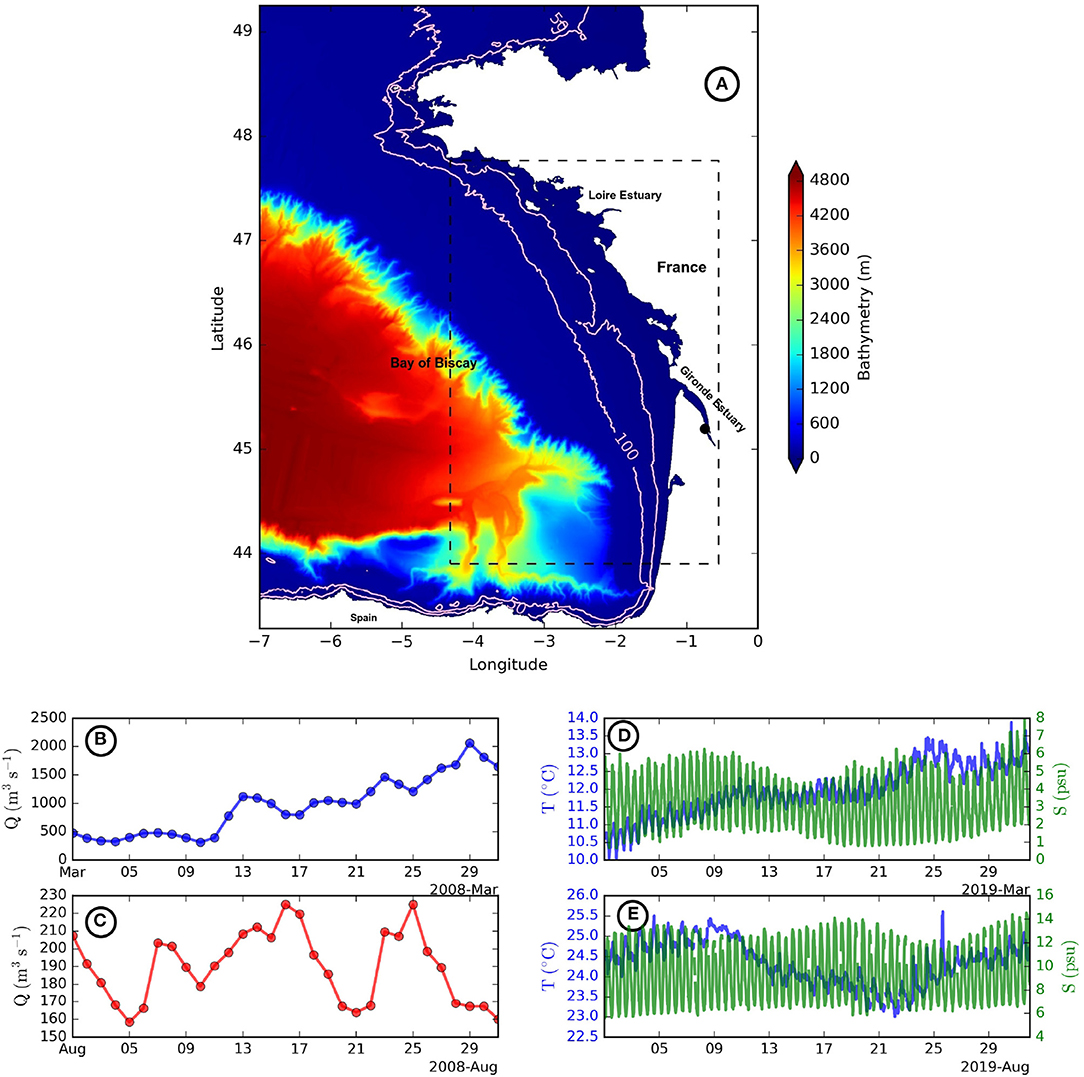
Figure 1. (A) Bathymetry of the Bay of Biscay used in numerical simulations; black dashed box limits the studied region; pink solid contours for the 50 and 100 m isobaths and the black dot in the estuary shows the Pauillac station. Daily values of the Gironde river discharge in March (B) and August (C). Time series of the temperature and salinity measured in the Gironde river estuary at the Pauillac station in March (D) and August (E).

The horizontal and vertical advection of momentum are performed with the Total Variation Diminishing scheme. The tracers horizontal and vertical advection schemes are with the Zico extension fifth order WENO scheme (a weighted ENO with improvements of the weights formula) (Rathan and Naga Raju, 2018). The tracer horizontal advection is rotated along isopycnals. The model turbulent closure scheme is KPP (Large et al., 1994). The background vertical diffusivities (for both momentum and tracers) are $\text{K}{\text{v}}_{\text{b}}=10^{-5}{\text{m}}^2{\text{s}}^{-1}$ and $\text{K}{\text{t}}_{\text{b}}=10^{-6}{\text{m}}^2{\text{s}}^{-1}$. Smagorinsky-like viscous and diffusive terms (with molecular viscosities and diffusivities) are implemented. The quadratic Von-Karman law (logarithmic law) is used for bottom friction with a bottom roughness z₀ = 5 mm.

Initial conditions and open boundaries are extracted from a daily average of the BACH1000, 1 km resolution, 100 sigma layers, MARS3D simulation (Charria et al., 2017; Akpınar et al., 2020). Open boundaries are parameterized using the Chapman (Chapman, 1985) and Flather scheme (Marchesiello et al., 2001) for 2D components (sea surface height and barotropic velocities). An Orlanski scheme is used for the 3D momentum and tracers (Orlanski, 1976). A sponge layer with 200 grid points is used.

Atmospheric forcing is provided by ERA-Interim (3 h) (Dee et al., 2011). The wind stress is computed from the C_d drag coefficient, model SST, and wind velocities at 10 m using the bulk formulae. The different components of the air-sea heat exchanges are parameterized using bulk definitions. The bulk formulation is based on air temperature, pressure, relative humidity at 2 m, rain and cloud coverage (ERA-Interim). The tidal sea surface elevation and currents with 15 harmonic constituents are imposed along the boundaries using the FES2014 ocean tide atlas (Lyard et al., 2020). In the result section, model outputs are detided using Godin filtering (Godin, 1972). In our study, 2 months (March and August 2008) have been simulated.

The freshwater source salinity and temperature for the Gironde river are estimated as monthly averages (March, August 2019) from the MAGEST in situ observing network time series (at 1 m depth; Figures 1D,E). Since no MAGEST data were available during the 2008 year, we chose the nearest year where freshwater source salinity and temperature are available (the 2019 year). The Pauillac station was considered here (location shown in Figure 1A) for summer and winter simulations. For the Loire river, temperature and salinity are estimated from the BOBYCLIM climatology (http://www.ifremer.fr/climatologie-gascogne/; Vandermeirsch et al., 2010). River discharges are provided by Banque Hydro France for Dordogne, Garonne (Gironde as a combination of both Dordogne and Garonne rivers) and Loire rivers, and their daily values are shown in Figures 1B,C. River inputs (discharge, freshwater source salinity, and temperature) are applied over one grid point at the end of the Gironde and Loire estuaries.

2.2. Methods of Analysis

2.2.1. River Plume Instabilities

The instability mechanisms are analyzed using the transfer of kinetic and potential energy from the mean to the turbulent flows. A scale decomposition is performed (into mean and perturbations) on the velocity and buoyancy fields. We write $\text{u}=\overline{\text{u}}+{\text{u}}^{\prime }$ and $\text{b}=\overline{\text{b}}+{\text{b}}^{\prime }$. Overbar and prime denote temporal mean over one day as follows ($\overline{\text{X}(\text{t})}=\frac{1}{\text{T}}{\int }_{\text{t}-\text{T}/2}^{\text{t}+\text{T}/2}\text{ X}({\text{t}}^{\prime })\text{d}{\text{t}}^{\prime }$) and perturbations relative to the mean flow, respectively. The horizontal (HRS) and vertical (VRS) shear stresses and the vertical buoyancy flux (VBF) (instantaneous values) are expressed as (Gula et al., 2016):

$\begin{array}{ll}\text{HRS}=-{\text{u}\prime }^2{\partial }_{\text{x}}\overline{\text{u}}-{\text{u}}^{\prime }{\text{v}}^{\prime }\left[{\partial }_y\overline{\text{u}}+{\partial }_{\text{x}}\overline{\text{v}}\right]-{\text{v}\prime }^2{\partial }_{\text{y}}\overline{\text{v}}& (1)\end{array}$

$\begin{array}{ll}\text{VRS}=-{\text{u}}^{\prime }{\text{w}}^{\prime }{\partial }_{\text{z}}\overline{\text{u}}-{\text{v}}^{\prime }{\text{w}}^{\prime }{\partial }_{\text{z}}\overline{\text{v}}& (2)\end{array}$

$\begin{array}{ll}\text{VBF}={\text{w}}^{\prime }{\text{b}}^{\prime }& (3)\end{array}$

Positive HRS, VRS, and VBF values indicate the potential presence of barotropic, vertical shear, and baroclinic instabilities, respectively. A positive HRS [transfer from MKE (mean kinetic energy) to EKE (eddy kinetic energy)] characterizes barotropic instability. A positive vertical buoyancy flux (VBF, transfer from potential to kinetic energy) reveals baroclinic instability. Mixed barotropic and baroclinic instabilities occur when VBF and HRS are positive at the same location. Kelvin-Helmholtz instability is characterized by a positive VRS. More generally, negative values of VBF, VRS, HRS represent a contribution from the perturbation to the mean flow (Kang, 2015; Contreras et al., 2019).

The change of sign of Ertel potential vorticity (Q) (or of its anomaly with respect to a state of rest) is used to indicate instability. Ertel potential vorticity is written as:

$\begin{array}{ll}\text{Q}={\omega }_a.\nabla \text{b}& (4)\end{array}$

where ω_a = ∇ ∧ u + fk is the absolute vorticity and $\text{b}=-\text{g}\frac{\rho }{{\rho }_0}$ is the buoyancy (ρ₀ is the mean density in our domain).

To understand the relation between river plumes, stratification and shear mixing, we evaluate the Richardson Number:

$\begin{array}{ll}{\text{R}}_{\text{i}}=\frac{{\text{N}}^2}{{\text{S}}^2}& (5)\end{array}$

where ${\text{N}}^2={\partial }_{\text{z}}\text{b}$ is the Brunt-Vaisala frequency and ${\text{S}}^2={\partial }_{\text{z}}{\text{u}}^2+{\partial }_{\text{z}}{\text{v}}^2$ is the vertical shear of horizontal velocity. R_i < 0.25 indicates the possibility of Kelvin Helmholtz instability (which is one type of vertical shear instability).

The Hoskins (1974) criteria fQ < 0) and R_i < 1 indicate a potential existence of symmetric instability.

Eddy kinetic energy [EKE = 0.5*(u^′2+v^′2)] was decomposed over different modes of instability as suggested by Stone's theory (Stone, 1970). We decompose perturbations using Fourier analysis onto baroclinic (BC), symmetric (SI), mixed modes (MM; as in Stamper and Taylor, 2016); MM are a combination of SI and BC. We consider the baroclinic mode in the cross-shore direction (independent of the wavenumber l) and the symmetric mode in the along-shore direction (independent of the wavenumber k); the mixed mode is for both directions (wavenumbers different than 0). We express the vertical averaged eddy kinetic energy associated with each mode as follows:

$\begin{array}{ll}{\overline{\text{EKE}}}^{\text{z}}(\text{k}=0,\text{l}\ne 0)={\displaystyle \frac{1}{2\text{H}}\int \int {\text{u}}^{\prime 2}+{\text{v}}^{\prime 2}\text{dldz}}& (6)\end{array}$

$\begin{array}{ll}{\overline{\text{EKE}}}^{\text{z}}(\text{l}=0,\text{k}\ne 0)={\displaystyle \frac{1}{2\text{H}}\int \int {\text{u}}^{\prime 2}+{\text{v}}^{\prime 2}\text{dkdz}}& (7)\end{array}$

$\begin{array}{ll}{\overline{\text{EKE}}}^{\text{z}}(\text{k}=\ne 0,\text{l}\ne 0)={\displaystyle \frac{1}{2\text{H}}\int \int \int {\text{u}}^{\prime 2}+{\text{v}}^{\prime 2}\text{dkdldz}}& (8)\end{array}$

Where we express perturbations as:

$\begin{array}{ll}{\text{u}}^{\prime },{\text{v}}^{\prime }=(\text{u}(\text{z}),\text{v}(\text{z}))*exp(\sigma \text{t})*exp\text{i}(\text{kx }+\text{ ly})& (9)\end{array}$

H represents the averaged depth of the base of the plume and is expressed as follows (Thomson and Fine, 2003):

$\begin{array}{ll}\text{mld}=\frac{\int \text{z}{\text{N}}^2\text{dz}}{\int {\text{N}}^2\text{dz}}& (10)\end{array}$

For each instability, the growth rate σ of instability is expressed as:

$\begin{array}{ll}\sigma =\frac{1}{2({\text{t}}_{\text{i}}-{\text{t}}_{\text{i}-1})}\text{log}(\frac{\text{EK}{\text{E}}_{\text{i}}}{\text{EK}{\text{E}}_{\text{i}-1}})& (11)\end{array}$

The same decompositions are performed on the EAPE (Eddy Available Potential Energy) field (Roullet et al., 2014)

$\begin{array}{ll}\text{EAPE}=\frac{{\text{b}}^{\prime 2}}{2{\text{N}}^2}& (12)\end{array}$

where b′ is the buoyancy perturbation field.

2.2.2. Analysis of the River Plume Restratification

We evaluate the ocean restratification in terms of PV mixing and of frontogenesis/frontolysis (Marshall and Nurser, 1992; Marshall et al., 2001; Lapeyre et al., 2006; Thomas and Ferrari, 2008). To describe PV mixing near the surface, we write the evolution equation of PV:

$\begin{array}{ll}{\partial }_{\text{t}}\text{Q}+\nabla .\text{J}=0& (13)\end{array}$

where the flux is written J = wq + ∇b ∧ F − ω_aD. The first term is advective stirring (Ja = wq), the second term is frictional mixing (Jf = ∇b ∧ F) and last term is diabatic mixing (Jd = −ω_aD). We write $\text{D}=\frac{\text{Db}}{\text{Dt}}={\partial }_{\text{t}}\text{b}+\text{u}{\partial }_{\text{x}}\text{b}+\text{v}{\partial }_{\text{y}}\text{b}+\text{w}{\partial }_{\text{z}}\text{b}$. F represents body forces in the Navier-Stokes equations as expressed in Marshall and Nurser (1992).

At the surface, advective stirring can be neglected (via the Haynes and McIntyre impermeability theorem) and we can write J = Jf + Jd = Jwind + Jttw + Jd_buoy + Jbot.

The frictional term is made of the wind contribution at the surface (Jwind) and of the body force exerted by the bottom (Jbot). The diabatic term is made of the surface buoyancy flux (Jd_buoy) and of a wind-driven buoyancy flux term at fronts (Jttw, where ttw stands for turbulent thermal wind), where Ekman transport can advect dense water over light one (e.g., Thomas and Ferrari, 2008). These four terms are expressed as follows:

$\begin{array}{ll}\text{Jwind}=(\text{f}+{\zeta }_{\text{z}})\frac{\text{EBF}}{\text{H}}& (14)\end{array}$

$\begin{array}{ll}\text{Jttw}=(\text{f}+{\zeta }_{\text{z}})\frac{\text{EB}{\text{F}}_{\text{g}}}{\text{H}}& (15)\end{array}$

$\begin{array}{ll}\text{J}{\text{d}}_{\text{buoy}}=(\text{f}+{\zeta }_{\text{z}}){\text{B}}_0\text{H}& (16)\end{array}$

$\begin{array}{ll}\text{Jbot}=\nabla \text{b}\wedge {\text{F}}_{\text{b}}.\text{n}& (17)\end{array}$

where $\text{EBF}={(\rho \text{f})}^{-1}{\tau }^w\wedge k.{\nabla }_h\text{b}$ (τ_w for the surface wind stress) is the Ekman Buoyancy flux. EBF_g = −ν∂_zu.∂_zu_g is the geostrophic Ekman buoyancy flux. Geostrophic shear is deduced from thermal wind balance, using ν = 0.1Hu^*, a scaling where ${\text{u}}^{*}=\sqrt{\frac{\left|\right|{\tau }^w\left|\right|}{\rho }}$ is the wind frictional velocity (Wenegrat et al., 2018). B₀ is the surface buoyancy flux deduced from D = ∂_zB. F_b represents the body force (the right hand side terms of the Navier-Stokes equations) at the bottom.

We focus on the restratification processes using a Budget of vertical density gradient (Brunt Vaisala frequency). This budget is related to PV fluxes (deduced from a volume integral of Equation 13) and frontogenesis [FRONT = ∂_t(ζ_zb), where ζ_z is the vertical component of the relative vorticity and b is the buoyancy]. This budget is defined as in Wenegrat et al. (2018) but we include the lateral transport of N² across the lateral boundaries since the computation domain is finite and subject to tides and river discharge from the estuary; it is written as:

$\begin{array}{l}{\partial }_{\text{t}}\overline{{\text{N}}^2}+\frac{\text{bvp}{|}_{{\text{z}}_{\text{b}}}^{{\text{z}}_{\text{t}}}}{\text{h}}=-\frac{1}{fh}(<FRONT>{|}_{z_b}^{z_t}+<J_d>{|}_{z_b}^{z_t}\\ +<J_f>{|}_{z_b}^{z_t}+<J_a>{|}_{z_b}^{z_t})& (18)\end{array}$

where $\overline{{\text{N}}^2}=\frac{<\text{b}(\text{z}={\text{z}}_{\text{t}})-\text{b}(\text{z}={\text{z}}_{\text{b}})>}{\text{h}}$; bvp is the boundary value problem considered here for the advection of N² across the lateral boundaries (called Σ); it is expressed as $\text{bvp}=\frac{1}{\Sigma }\int \int \text{u}.\text{n}{\text{N}}^2\text{d}\Sigma$. h represented the thickness (z_t - z_b) of the layer where this budget is evaluated. The brackets (< >) indicate a horizontal averaging over a domain. In our study, this budget is evaluated near the surface and in the frontal region of the Gironde plume.

3. Model Validation

3.1. Frontal Dynamics

In this section, the modeled salinity is described for the two simulated months (March and August). Here the salinity evolution is not detided. The horizontal salinity gradients are derived and compared with MODIS chlorophyll concentration gradients (with ~800 m spatial resolution); this comparison of two different tracers aims at comparing the fronts. Indeed, remotely sensed salinity is not available at high resolution.

First, the spatial distribution of the salinity is explored in the studied region (Figures 2A,B). The Gironde river plume is made of two regions: a bulge (an anticyclonic gyre near the river mouth, also called the near field) and a coastal current (also called the far field). When the river discharge rate is nominal (~1,500 m³ s⁻¹), the Gironde river plume is well developed (for instance, in March 2008). Low salinity water from the estuary is advected offshore in the plume, and extends northward, up to a latitude ~ 46.5°N, via the coastal current. Indeed, low salinity values (with values of about 30) characterize the river water in the open ocean, once it has exited the estuary. This plume remains close to the coast due to wind influence. By contrast, in August, the bulge is small because of the low river discharge (200 m³ s⁻¹), and of strong westerlies. Indeed, these westerlies favor the development of a northward coastal current. They constrict the coastal current near the coast while it extends to the northern part of the domain. The plume is bounded by sharp salinity gradients with the high salinity shelf water (34–35 psu). These gradients are observed to oscillate with tides.

FIGURE 2

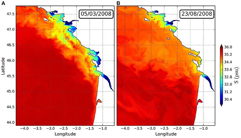
Figure 2. Modeled sea surface salinity at midnight on March 5 (A) and on August 23 (B) 2008.

Figure 3 shows the horizontal salinity gradient and MODIS chlorophyll gradient in the studied region. The salinity gradient is mainly zonal as ∂_xS > ∂_yS. In March, salinity fronts are intense inside and outside of the Gironde estuary (Figure 3A). Near the Gironde river mouth, they remain close to the coast (longitude ~ 1.5°W). These fronts are more sensitive to the average river discharge. The river discharge also feeds the coastal current where salinity fronts are intense. In the Gironde river plume, the zonal salinity gradient is largest in the estuary since the river discharge is low in August (Figure 3B). In the near field, the Gironde river plume front remains close to the coast (longitude ~1.5°W). This plume extends to the north (up to a latitude ~46.5 °N) in the coastal current. Moderate winds and small river discharge constrict the coastal current near the coast. Beyond the river plume front, small scale filaments and eddies are observed.

FIGURE 3

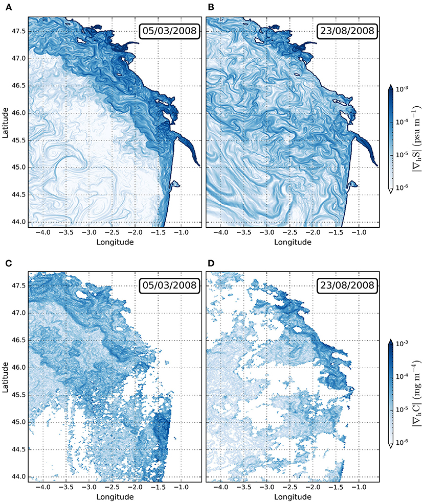
Figure 3. Modeled sea surface salinity gradients the 5 March (A) and the 23 August (B) 2008; and corresponding observed Sea Surface Chlorophyll-a gradients in March (C) and in August (D) from MODIS satellite.

Then, we compare these modeled salinity fronts to observed chlorophyll fronts (Figures 3C,D). In winter, cloud coverage does not allow the observation of the Gironde river plume (Figure 3C). Thus, comparisons are carried out outside of this region. South of the Gironde river plume (latitude between 44.5 and 45°N), the observed chlorophyll fronts and modeled salinity fronts locations are similar (longitude ~1.6°W). On the northern side of the bay, the Loire river plume front (latitude ~47°N) remains close to the coast in our numerical simulation and in the observed MODIS dataset. The modeled and observed river plume fronts are different in intensity. The location of salinity and chlorophyll fronts is similar outside of the Loire river plume. In August, the turbid Gironde river plume and salinity fronts are similar (Figure 3D). In the near field, the chlorophyll gradient maxima is close to the coast (longitude ~1.5°W). Meanwhile, the chlorophyll front is at the same longitude in the coastal current.

Thus, our numerical simulations reproduce the frontal activity linked with the salinity gradients in the studied region. The main differences between the model and the data are that: (i) in the Gironde river plume, the coastal plume front is closer to the coast in numerical simulations, (ii) small scale eddies and filaments outside the Gironde river plume are not observed in the MODIS dataset. These differences can be due to: (i) different horizontal resolutions, (ii) MODIS chlorophyll data is influenced by biological processes, (iii) uncertainties in MODIS chlorophyll data due for instance to cloud coverage, or (iv) the fact that we include only the Loire and Gironde rivers in our numerical simulations. Other rivers, such as the Charente and the Sèvre-Niortaise, located between the Loire and Gironde rivers, may contribute to the total freshwater input and change slightly the coastal current front location due to their small discharges (between 12 and 40 m³ s⁻¹ in annual average).

3.2. Tidal Dynamics in the Model Simulations

Here, we compute the modeled and observed sea surface height (ssh) anomaly. The ssh anomaly (ssha) is computed as the perturbation from a time mean over the studied periods. Then, we decompose these signals into different tidal harmonics. This decomposition is performed on each tidal constituent and written as

$\begin{array}{ll}\text{ssha}(\text{t})={\displaystyle \sum _{\text{i}=0}^{\text{k}}}{\text{a}}_{\text{i}}\text{cos}({\omega }_{\text{i}}\text{t}+{\varphi }_{\text{i}})& (19)\end{array}$

where a_i are the Fourier coefficients, ω_i is the angular frequency of harmonic i and ϕ_i is its phase.

These decomposed signals are extracted at four locations across the domain. These locations are listed in Table 1. In our numerical simulations, we consider the nearest immersed locations to observations. This validation is performed for semi-diurnal (M2, S2, and N2) and for diurnal (K1, O1, Q1) tidal constituents. The amplitudes and phase lags averaged over all tidal gauges for observations and numerical model are first explored (Figure 4). The main differences are observed for the semi-diurnal components with an amplitude overestimated by the model of the M2 and N2 harmonics (+~10 cm in August and March) and an underestimation of the S2 harmonic (−5 to 10 cm) (Figure 4A). Simulated diurnal components are close to observations with differences around 1 cm (an underestimation by the model of the O1 harmonic amplitudes by 1 cm, an overestimation of the K1 harmonics by 1–2 cm for both months, with differences of 0.5–1 cm for Q1 harmonic).

TABLE 1

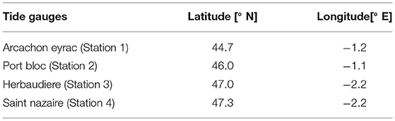
Table 1. Geographic location of each tide gauge in the studied domain.

FIGURE 4

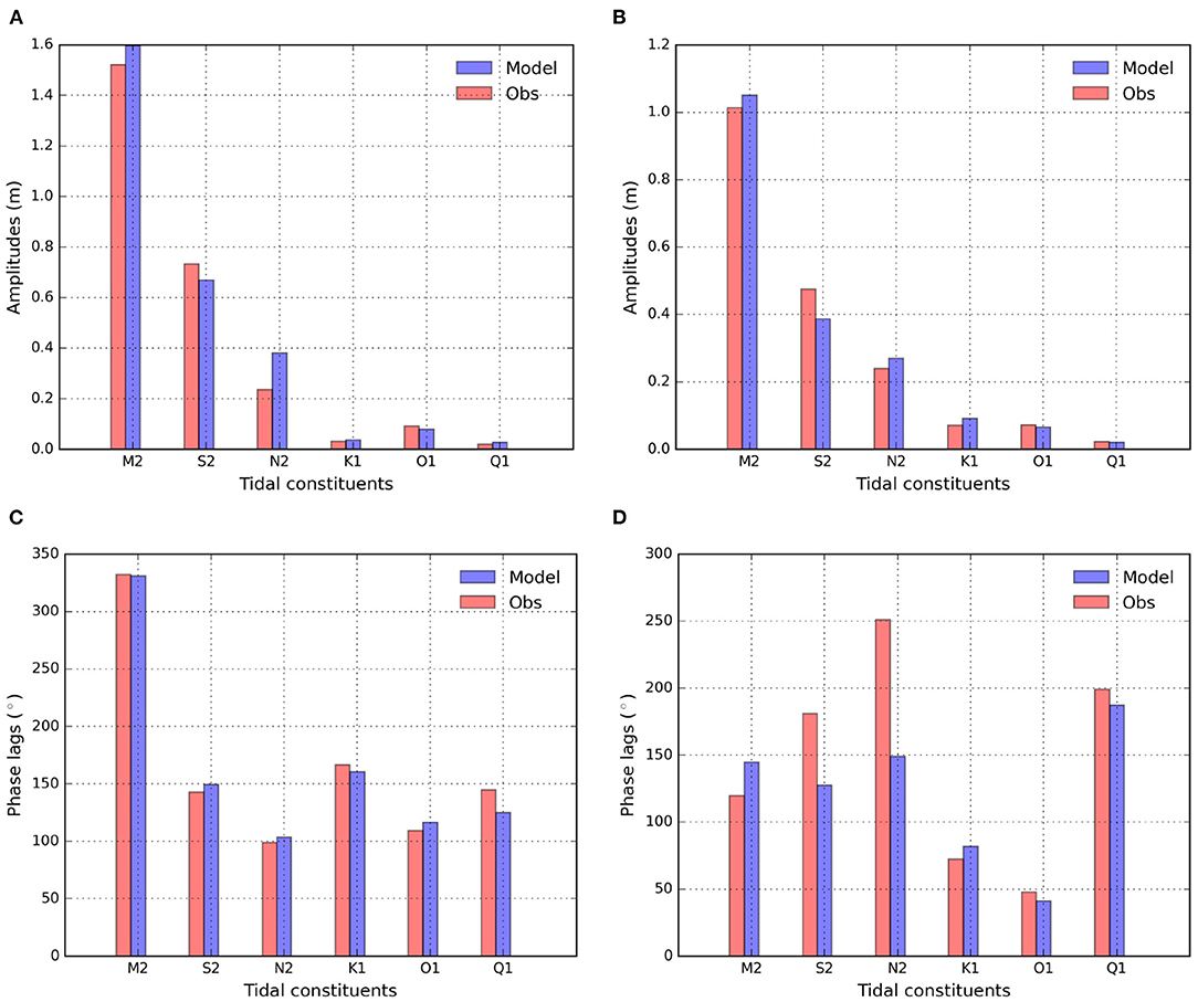
Figure 4. Statistics of the mean tide amplitudes in March (A) and in August (B) from numerical simulations (blue) and tide gauge observations (red); and the corresponding mean phase lags in March (C) and August (D) averaged using four tide gauges (see Table 1).

In March, the model overestimates the phases lags of several tidal constituents: S2 by 1°, N2 by 1°, and O1 by 2° (Figure 4B). It underestimates the M2 by 1°, K1 by 2°, and Q1 by 10° tidal constituents in phase lags. In contrast, during August the model underestimates the S2 by 30°, N2 by 100°, O1 by 5°, and Q1 by 10° tide harmonics as phases lags. But it overestimates the phase lags of the M2 by 20° and K1 by 10° harmonics. In order to evaluate these discrepancies two statistical indicators are defined, the root mean square error (RMSE) and the Willmott refined index (d_i) that we write as

$\begin{array}{ll}\text{RMSE}=\sqrt{\frac{1}{\text{n}}{\displaystyle \sum _1^{\text{n}}}{({\text{P}}_{\text{i}}-{\text{O}}_{\text{i}})}^2}& (20)\end{array}$

$\begin{array}{ll}{\text{d}}_{\text{i}}=1-\frac{{\displaystyle {\sum }_1^{\text{n}}}|{\text{P}}_{\text{i}}-{\text{O}}_{\text{i}}|}{2{\displaystyle {\sum }_1^{\text{n}}}|{\text{O}}_{\text{i}}-\overline{{\text{O}}_{\text{i}}}|}& (21)\end{array}$

when $\sum _1^{\text{n}}|{\text{P}}_{\text{i}}-{\text{O}}_{\text{i}}|\le 2\sum _1^{\text{n}}|{\text{O}}_{\text{i}}-\overline{\text{O}}|$

$\begin{array}{ll}{\text{d}}_{\text{i}}=\frac{2{\displaystyle {\sum }_1^{\text{n}}}|{\text{O}}_{\text{i}}-\overline{{\text{O}}_{\text{i}}}|}{{\displaystyle {\sum }_1^{\text{n}}}|{\text{P}}_{\text{i}}-{\text{O}}_{\text{i}}|}& (22)\end{array}$

when $\sum _1^{\text{n}}|{\text{P}}_{\text{i}}-{\text{O}}_{\text{i}}|>2\sum _1^{\text{n}}|{\text{O}}_{\text{i}}-\overline{\text{O}}|$

where the overbar denotes a time average over the studied period and n refers to the number of values for the observed and modeled time series.

The RMSE evaluates the bias between the modeled (P_i) and the observed (O_i) ssh anomaly signals. The refined Willmot index characterizes the performance of the model to predict the observed values and it is bounded between −1 and 1 (Willmott et al., 2012). The refined Willmott index is less sensitive to outliers. These indicators are computed for each tide gauge and constituent. The RMSE of ssh anomaly is <12 cm at each station for the semi-diurnal tidal constituents in March and August (Figures 5A,B). This indicator is above 10 cm for the N2 harmonic during these periods. The RMSE between observations and model ssh anomaly is between 0.5 and 2 cm at each location in March and August for the diurnal tidal constituents. It reaches a maximum of 2 cm for the K1 harmonic near the Gironde (Station 2) and the Loire (Station 3) river plumes in August. The Willmott refined index indicates that the model performance at each location is good (d_i ≥ 0.7) for most of the semi-diurnal and diurnal tidal constituents in March and August (Figures 5C,D). However, the agreement between the numerical and observations is correct (0.5 ≤ d_i < 0.7) for the N2 harmonic at the 4 stations in March, and near the Gironde river plume (Station 2) in August. This satisfactory performance is also observed for the Q1 harmonic near the Gironde river plume (Station 1). A poor performance of the model (0 ≤ d_i < 0.5) is observed for the Q1 harmonic at station 1 (near the Gironde river plume) in March. Finally, the model outperformed (d_i < 0) for the M2 and N2 harmonics near the Loire river plume (Station 3) in August.

FIGURE 5

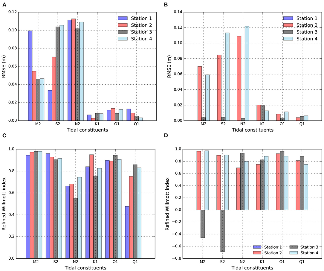
Figure 5. RMSE in March (A) and in August (B); and the refined Willmott index in March (C) and in August (D) between the modeled and observed Sea Surface Height anomaly for each station (detailed in Table 1) and M2, S2, N2, K1, O1, and Q1 tidal constituents.

The differences between observed and modeled sea level can be explained by: (i) the location of the tide gauges near the coast, or near islands, where the model grid is too coarse to resolve local processes, or (ii) the sensitivity to the bottom drag parameterization in the numerical model. Simulated tides are sensitive to the bathymetry, the bottom roughness and to the friction law (linear, quadratic, and logarithmic) (Toublanc et al., 2018; Piton et al., 2020).

Despite these differences and since the Bay of Biscay is energetic in M2 and S2 tidal harmonics, the numerical model performance is satisfactory for the simulations of tides.

3.3. Vertical Salinity Structure

Now, we evaluate the salinity distribution in the numerical simulations of March and August 2008, in order to explore the Gironde river plume dynamics. We use observations from cruises carried out during these periods. ECLAIR cruises (Huret et al., 2018) located in front of the Gironde estuary, and achieved in March (10–16th) and August (10–14th) 2008 constitute a unique and valuable dataset to validate the vertical salinity structure in our simulations. The vertical salinity profiles from 13 CTD stations are compared with colocated modeled profiles (Figure 6). During the ECLAIR1 cruise in March 2008, a river plume with a limited offshore extent was observed despite the high river discharge season. Profiles 2 and 4 (Figure 6) show comparable salinity values with a similar stratification (profile 2 has a lower salinity at the surface originated from the plume). The model overestimates the salinity (+0.1 in profile 2 in the surface layer; +0.1 in profile 4 outside the plume in a vertically mixed water column). In summer, during ECLAIR5, the modeled river plume extends offshore with several low salinity filaments. The river plume reaches a depth of about 30 m (profiles 7 and 13) in the numerical simulation, similar to the observed profiles. In the plume, low salinities between 34.4 and 34.6 are reproduced in the simulations. Deeper, below 40 m depth, the observed and simulated salinities are very close with values around 35.6. The large spatial and temporal variability of the river plume makes the comparison to in-situ observations complicated. However, the simulated salinity and vertical gradients are in good agreement with the observations which make us confident about the realism of our simulations of the plume.

FIGURE 6

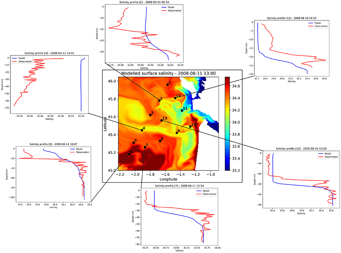
Figure 6. Map of the simulated surface salinity for the 11th August 2008 including station positions of ECLAIR cruises in 2008. Example of associated individual salinity profiles (blue—modeled, red—observed) in March (stations 2 and 4) and in August (stations 6, 7, 12, and 13).

4. Analysis of the Gironde River Plume Structure, Stability, and Mixing

4.1. Gironde River Plume Dynamics

The dynamics of the Gironde river plume is first analyzed using the local Rossby number (R_o ~ $\frac{{\zeta }_{\text{z}}}{\text{f}}$, where ζ_z is the vertical component of the relative vorticity and f the Coriolis parameter) at the surface; this is presented in Figure 7. This local Rossy number determines the geostrophic or ageostrophic nature of the velocity field of the Gironde river plume. In winter (March), the circulation is mostly anticyclonic in the plume (ζ_z < 0) except : (i) at the river mouth (longitude ~1.2°W and latitude between 45.5 and 45.6°N), (ii) in the northern part of the coastal current (longitude ~1.5°W and latitude ~ 46.2°N), and (iii) offshore of the plume front (longitude ~ 1.5°W and latitude between 45.75 and 46.2°N; Figure 7, left). The circulation is ageostrophic [R_o ~ O(1)] at these locations. Moreover, strong negative vorticity ($\frac{{\zeta }_{\text{z}}}{\text{f}}$ < −1) is observed in the coastal current. Further offshore, over the continental shelf, the local Rossby number is small, indicating a geostrophic balance. In contrast, when the ocean is stratified (in August), the circulation remains anticyclonic in the river plume except : (i) at the northern corner of the river mouth (longitude ~1.2°W and latitude ~45.6°N), (ii) near the coast south of the Gironde river plume (longitude between 1.2 and 1.5°W and latitude between 45 and 45.4°N), and (iii) at the offshore edge of the plume front (longitude ~ 1.5°W and latitude between 45.4 and 46.2°N; Figure 7, right). This (cyclonic) circulation is ageostrophic at the northern (latitude between 45.75 and 46°N) and southern edges of the plume front and in a small filament south of the Gironde, along the coast and to the east. At the southern edge of the plume, a small ageostrophic cyclonic eddy can be observed (longitude ~1.5°W and latitude ~45.4°N) due to recirculation processes. Over the continental shelf and outside of the Gironde river plume, the overall circulation is anticyclonic except at the rim of small eddies and in filaments. The stratification in summer favors the development of anticyclonic eddies over the continental shelf.

FIGURE 7

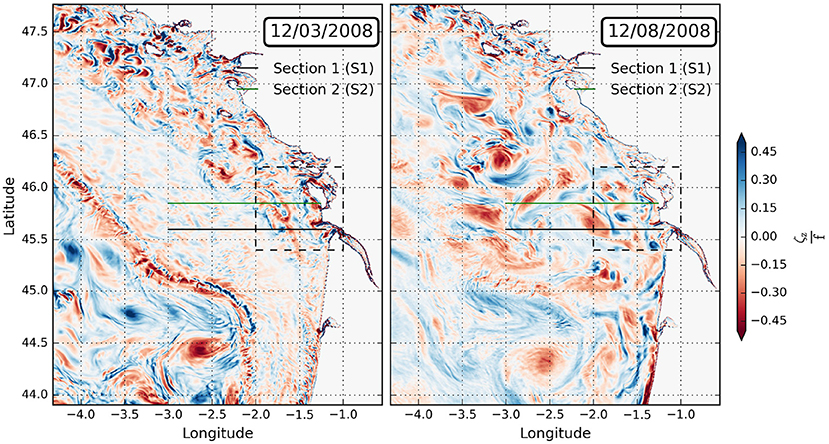
Figure 7. Surface local Rossby number in March (left) and in August (right) 2008. The black dashed box shows the analyzed delimited region in Figures 8, 12, 15. The green and black solid lines show the vertical sections represented in Figures 9, 10.

Despite the existence of local ageostrophic motions in the Gironde river plume and over the continental shelf, on average (over the box in Figure 7), the global Rossby number is small (R_o ~ 0.1) both in March and August. This means that the global circulation over the continental shelf is mostly in geostrophic balance. Therefore, to understand the contrast between these motions, we represent in Figure 8 the surface averaged time evolution of the wind stress intensity ($\tau =\sqrt{{\tau }_{\text{x}}^2+{\tau }_{\text{y}}^2}$, where τ_x and τ_y are the cross-shore and along-shore wind stress components) and the vertical geostrophic shear. These terms are evaluated in frontal regions bounded by two isopycnals (1,024 and 1024.5 kg m⁻³ in August, 1,025 and 1025.5 kg m⁻³ in March) and are written as

$\begin{array}{ll}{\text{S}}_{\text{g}}^2={\partial }_{\text{z}}{\text{u}}_{\text{g}}^2+{\partial }_{\text{z}}{\text{v}}_{\text{g}}^2=\frac{{\partial }_{\text{y}}{\text{b}}^2+{\partial }_{\text{x}}{\text{b}}^2}{{\text{f}}^2}& (23)\end{array}$

where $\text{b}=-\text{g}\frac{\rho }{{\rho }_0}$ is the buoyancy (g is the gravity acceleration, ρ is the potential density and ρ₀ is a mean density over the studied domain), and the vertical ageostrophic shear is written as

$\begin{array}{ll}{\text{S}}_{\text{ag}}^2={\partial }_{\text{z}}{(\text{u}-{\text{u}}_{\text{g}})}^2+{\partial }_{\text{z}}{(\text{v}-{\text{v}}_{\text{g}})}^2& (24)\end{array}$

In March, a storm is observed during the first half of the month (between March 9th and 13th; Figure 8A). During this period and after a lag of ~ 1 day, the vertical ageostrophic shear increases and the geostrophic shear remains steady (Figures 8B,C). Then (between 13 and 15th March), a wind relaxation event is observed during which the ageostrophic shear slackens and the geostrophic shear increases. Afterwards (between 15 and 21st March), the geostrophic shear weakens and remains steady during 3 days. Conversely, during the latter period, few moderate wind events are observed with few variations in the ageostrophic shear. Following this period (between 21 and 23rd March), weak wind events are associated with the growth of geostrophic shear and weak ageostrophic shear. At the end of March, the geostrophic shear decreases noticeably and a weak maximum in the ageostrophic shear is observed. Geostrophic shear growth events are associated with wind relaxation and increase in river discharge (Q ~ 1,000 and 1,500 m³ s⁻¹, see Figure 1B). Meanwhile, the wind conditions in August 2008 are characterized by a series of strong wind events, with an intensity larger than the peak in March (an order of magnitude larger). Therefore, the ageostrophic component predominates largely over the geostrophic shear (an order of magnitude larger) due to these wind conditions and to the weak river discharge during this period (Q ~ 200 m³ s⁻¹, see Figures 1C, 8D). The increase of the ageostrophic shear during this month is due to previous wind gusts (Figure 8F). Moreover, the geostrophic shear increases during wind relaxation events or when the ageostrophic shear slackens (Figure 8E). It remains quasi-steady during periods where the ageostrophic shear increases.

FIGURE 8

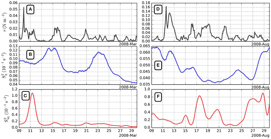
Figure 8. Wind stress intensity in March (A) and in August (D). Geostrophic shear in March (B) and in August (E). Ageostrophic shear in March (C) and in August (F). These quantities are averaged over the box shown in Figure 7 and between two isopycnals as explained in the text.

Thus, ageostrophic motions prevail in the frontal region of the plume due to (i) a local Rossby number R_o ~ O(1) and (ii) higher (two times larger in March or an order of magnitude larger in August) ageostrophic shear than the geostrophic shear (the geostrophic shear is an order of magnitude larger in March due to the average river discharge >1,000 m³ s⁻¹). In the Bay of Biscay, ageostrophic motions are more noticeable in winter (March) over the inner shelf (shallower than 100 m) and over the whole continental shelf in summer (August).

4.2. Generation and Occurrence of Instabilities in the Gironde River Plume

In this section, we perform diagnostics to identify and characterize instabilities in the Gironde river plume. First, we evaluate the existence of symmetric instabilities using the Hoskins stability criterion in the near field and the coastal current during March and August. The Hoskins stability criterion is based on negative PV values and a Richardson number smaller than one. Negative PV are related to different instabilities: gravitational, inertial (centrifugal), or symmetric. Gravitational instability requires unstable stratification (negative N²) which is not the case here since the Richardson number is positive (Figures 9E,F). Centrifugal instability requires a negative absolute vorticity which is not the case here either (figure not shown). Hereafter, we will refer to negative PV (Hoskins criteria) as symmetric instabilities since it is mostly dominated by geostrophic and ageostrophic shears. In March, symmetric instabilities exist in different locations of the near field: (i) in the Gironde river plume (longitude between 1.25 and 1.4°W) from the surface to the bottom, (ii) at the offshore edge of the river plume front (longitude ~1.5°W) where large (negative) values are observed near the surface (at 2 m depth), and (iii) offshore of the Gironde river plume (longitudes between 1.6 and 1.8°W) from 10 to 40 m depth (Figures 9C,E). In the plume interior, symmetric instabilities are generated via local flow interaction with moderate winds and river discharges inducing vertical sheared horizontal currents. In the offshore part of the plume front, they are also observed and intensified near the surface due to strong buoyancy/salinity gradients and high wind sheared flows since the vertical ageostrophic shear prevails there (see previous section). Offshore of the Gironde river plume, symmetric instabilities may exist from 10 m down to 40 m depth due to interior horizontal sheared currents and weak/homogenized stratification. Near the bottom, vertical shear instabilities may prevail, since the Richardson number is smaller than 0.25, due to high baroclinic tidal currents and steep bathymetric gradients which induce high sheared currents. In this region the freshwater density is lower than 1,026 kg m⁻³ and the plume is bottom attached (isopycnals interact with the bottom) (Figure 9A).

FIGURE 9

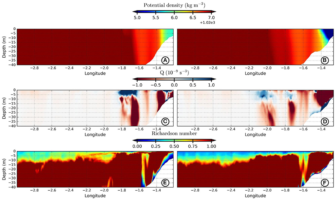
Figure 9. Snapshot (12/03/2008 at midday) of: the Potential density in section 1 (A) and in section 2 (B) (cf. Figure 7), the PV in section 1 (C) and in section 2 (D) and the Richardson number in section 1 (E) and in section 2 (F).

In March, in the coastal current, symmetric instabilities also exist at different locations: (i) near the coast (longitude between 1.3 and 1.5°W) in almost the whole water column except in a small layer near the bottom, (ii) at the edge of the plume (longitude ~ 1.6°W) between the surface and 25 m depth, and (iii) offshore of the plume (longitude between 1.7 and 2°W) between 15 and 40 m depth (Figures 9D,F). In the plume interior, symmetric instabilities are intensified near the surface (~ 5 m depth) via the interaction of the plume with winds, tidal currents and/or the coast. The plume interaction with winds and baroclinic tidal currents enhances the sheared currents intensity and therefore the vertical components of the PV become dominant which induce negative PV. The interaction between the coast and the Gironde plume may also induce processes which may favor the development of such instabilities. At the edge of the plume, symmetric instabilities prevail on the upper 25 m due to frontogenetic processes inducing high salinity gradients, baroclinic tidal currents, and moderate winds favoring intense ageostrophic vertical shear. Meanwhile, offshore of the Gironde plume, these instabilities exist on the upper 10 m via the ageostrophic shear induced by moderate winds. Near the bottom in this region of the plume, since the freshwater interacts with the bottom with densities <1,026 kg m⁻³ as seen in Figure 9B, vertical shear instabilities may dominate. The latter instabilities develop due to steep bottom slopes and baroclinic tidal currents which favor strong sheared flows.

In August, symmetric instabilities also exist at different locations of the near field region bounded by different isopycnals. In regions where the density is smaller than 1024.5 kg m⁻³ (Figure 10A), they exist at different longitudes: (i) between 1.4 and 1.6°W, (ii) between 1.8 and 2°W, and (iii) far offshore between 2.4 and 2.7°W. These instabilities span the vertical extent of the isopycnal layer, between the surface and 25 m depth (Figures 10C,E). Symmetric and vertical shear instabilities coexist from the surface down to ~10 m depth, since the Richardson number is smaller than 0.25 and the PV is negative, due to the wind activity inducing a high vertical shear. The river discharge would have a weak influence on those instabilities since small values (~) 200 m³ s⁻¹ are observed during August. In this isopycnic layer and slightly beneath, symmetric instabilities exist also due to shear interior induced by strong frontogenetic processes generated by tidal currents and/or internal waves. Near the bottom, symmetric and vertical shear instabilities coexist due to strong bathymetric gradients and baroclinic tidal currents.

FIGURE 10

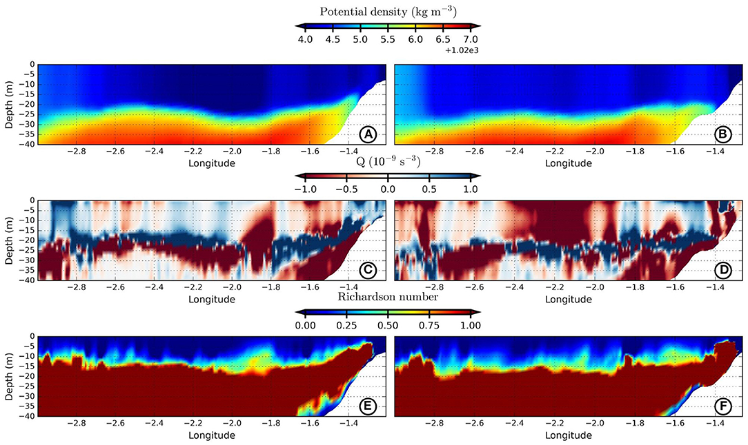
Figure 10. Snapshot August (12/08/2008 at midday) of: the Potential density in section 1 (A) and in section 2 (B) (cf. Figure 7), the PV in section 1 (C) and in section 2 (D) and the Richardson number in section 1 (E) and in section 2 (F).

In the coastal current and during the same period, symmetric instabilities prevail in regions with smaller densities, <1024.5 kg m⁻³ as shown in Figure 10B, and at various zonal locations: (i) near the coast (longitude ~ 1.4°W), (ii) between 1.6 and 1.8°W, (iii) between 1.9 and 2.4°W, and (iv) far offshore with longitudes >2.8°W (Figures 10D,F). These instabilities overwhelm almost the entire isopycnic layer and are more intense due to stronger wind bursts compared to a winter situation (an order of magnitude stronger). At the top 10 m, they coexist with vertical shear instabilities, since the Richardson number is smaller than 0.25, due to strong ageostrophic shear which engenders negative PV values. Symmetric instabilities also exist between 10 and 25 m depth in regards of the interaction between the ambient stratification and tidal currents which induce frontogenetic processes and therefore intense horizontal buoyancy gradients. Beneath this isopycnic layer and near the bottom, symmetric and vertical shear instabilities coexist (R_i < 0.25), from 1.4 to 1.6°W longitude, due to steep bottom slopes and tidal currents inducing high ageostrophic shear.

Energy conversion terms are evaluated near the surface, at 5 m depth, during both months to identify the existence and intensity of baroclinic, barotropic, and vertical shear instabilities (Figure 11). Positive HRS, VBF, and VRS indicate the existence of barotropic, baroclinic, and vertical shear instabilities, respectively. The VBF and HRS dominate over the VRS term near the river mouth (not shown—VRS values below 10⁻⁹ m s⁻³).

FIGURE 11

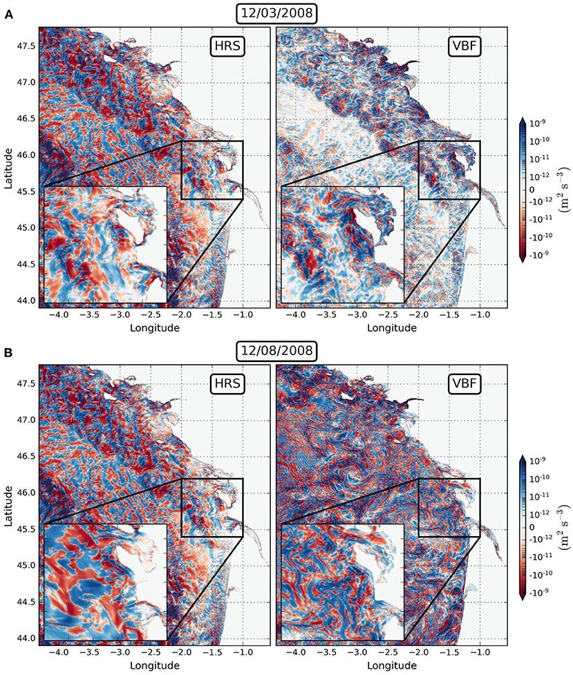
Figure 11. HRS and VBF energy conversion terms at 5 m in March (A) and in August (B) 2008. The left corner panel indicates a zoom on the region delimited by the black solid box centered on the Gironde river plume.

In winter, barotropic and baroclinic instabilities coexist at a larger scale over the continental shelf at the rim of eddies and in filaments (Figure 11A). Over the continental shelf, winds play a major role in increasing the energy of the mean flow which feeds the perturbations, and therefore the generation of mixed barotropic/baroclinic instabilities is observed. Over the inner-shelf (above 100 m isobath), these mixed instabilities are more intense due to the interaction of density currents induced by Gironde plume and its front, tidal currents and wind bursts. Those interactions sustain the mean flow (buoyancy and momentum) with a high reservoir of energy which feed the perturbations and generate such instabilities.

In summer, mixed barotropic/baroclinic instabilities exist in the near field and the coastal current of the plume, and over the continental shelf (Figure 11B). Compared to winter, those instabilities are intensified over the whole domain. In the Gironde plume and since the river discharge is weak, the source of such instabilities is the interaction of the ocean surface layer with tidal currents and wind activity. Those interactions alter the stratification and the momentum which induce perturbations essential to the generation of mixed barotropic/baroclinic instabilities. Over the continental shelf, the mean flow induced by eddies, wind bursts, and internal waves favor the development of these instabilities.

Since the wind and tides contribute to the generation of baroclinic and symmetric instabilities, the relation between these two instabilities in frontal regions of the plume will be explored in the following section.

4.3. Plume Instability

The development of instability can be monitored using the evolution of the energy from buoyancy and momentum perturbations. We then decompose the Eddy Kinetic Energy (EKE) and Eddy Available Potential Energy (EAPE) in three main contributions from: symmetric, baroclinic, and mixed instabilities (Figure 12).

FIGURE 12

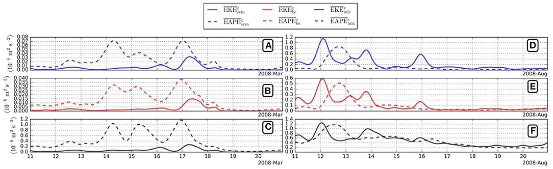
Figure 12. Decomposition of the EKE and the EAPE onto individual modes of instability : symmetric mode (blue color) in March (A) and in August (D), baroclinic mode (red color) in March (B) and in August (E) and mixed mode (black color) in March (C) and in August (F). The solid lines characterize the EKE decomposition and dashed lines indicate the EAPE decomposition.

In winter, the mixed modes are dominant in both decompositions of EKE and EAPE; they are one order of magnitude larger than the symmetric and baroclinic modes during the first 8 days (see Figures 12A–C).

Meanwhile, during the last 2 days of this analyzed period, the three modes feed equally and weakly the perturbations in the 3D eddying state. Through this decomposition, two events are noticed which occur during the second half of March (on the 16th and the 17th). During these periods, peaks in EAPE precede peaks in EKE with a lag of about half a day. The lag is similar for the symmetric and baroclinic modes.

Conversely in August, the symmetric, baroclinic, and mixed modes supply EKE and EAPE significantly with a predominance of the mixed perturbations (Figures 12D–F). During this period, three major events can be observed in the EKE decomposition. The first event occurs around August 12th. On this day, the mixed mode grows first with a significant amplitude followed by symmetric and then baroclinic modes. Then, a second event occurs almost 2 days later when the symmetric mode grows first followed by baroclinic and then mixed modes. On August 16th, symmetric and mixed modes contribute equally and nearly at the same time followed by baroclinic modes. Finally, after this active period the three unstable modes have developed nonlinearly and reach a 3D eddying state. In contrast, in the EAPE decomposition only the first event is noticeable. It occurs almost a day later. Similarly to the EKE decomposition, mixed modes increase first followed by symmetric and then baroclinic modes. The lag between EKE and EAPE suggests that a transfer of energy occurs within the same instability mode.

The development of these instabilities is related to the wind activity. A lagged cross-correlation between the EKEs and the wind stress intensity (~0.7) reveals that the instabilities develop after wind events within a lag ~18 h in summer and ~3 days in winter (figure not shown). These lags are different due to a larger wind stress intensity in summer (an order of magnitude larger compared to winter).

Growth rates can be deduced from the evolution of EKE (see Equation 11). Estimated growth rates (Figure 13) range from 0.02 to 0.12 h⁻¹ (i.e., time scales ranging from 8 to 50 h). In March, the second event grows faster and contributes more to the increase of the EKE (Figure 13A). Meanwhile in summer (Figure 13B), growth rates are higher for symmetric and baroclinic instabilities (between 0.04 and 0.08 h⁻¹ for symmetric instabilities and between 0.04 and 0.1 h⁻¹ for baroclinic instabilities). On the opposite, in winter, mixed and symmetric instabilities have higher growth rates (between 0.04 and 0.1 h⁻¹ for mixed instabilities and between 0.04 and 0.12 h⁻¹ for symmetric instabilities).

FIGURE 13

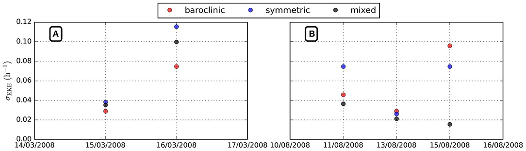
Figure 13. The EKE growth rate of each instability (baroclinic in red, symmetric in blue, and mixed in black) computed between midday (previous day) and midnight in March (A) and in August (B) 2008.

4.4. Mixing at Ocean Boundaries

To explore the mixing in different ocean layers, the potential vorticity (PV) mixing in Gironde river is first evaluated in the surface and bottom boundary layers, where the isopycnals can outcrop. We averaged over 10 days (between the 10th and the 20th of each month) the surface wind-driven, buoyancy, thermal turbulent wind, and bottom PV fluxes. These fluxes have been evaluated between two outcropping isopycnals (at the surface and at the bottom): between 1,025 and 1025.5 kg m⁻³ in March and between 1,024 and 1024.5 kg m⁻³ in August. Figure 14 shows the spatial distribution of these fluxes during the two periods.

FIGURE 14

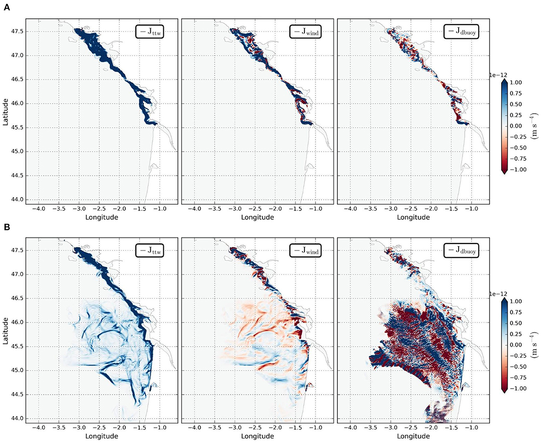
Figure 14. The PV fluxes: thermal turbulent wind (-Jttw), the wind-driven (-Jwind), and the surface buoyancy (-Jdbuoy) in March (A) and in August (B).

In March, surface buoyancy fluxes always remove PV from the ocean surface (-Jdbuoy <0) except at some locations: (i) at the Gironde river mouth (longitude ~1.5°W and latitude ~45.6°N) and (ii) at the northern edge of the coastal current (longitude ~1.5°W and latitude ~46.2°N) (Figure 14A). The wind-driven PV fluxes (-Jdwind) inject and remove potential vorticity from the surface depending on the location. They strongly remove PV at the northern edge of the coastal current and at the offshore edge of the plume. On the opposite, near the river mouth and in the inner edge of the plume front, wind-driven PV is injected. The thermal turbulent wind flux (-Jttw) always injects PV at the ocean surface, suggesting the importance of buoyant fronts induced by the Gironde river in the PV budget. These fluxes have comparable magnitudes (~10⁻¹² m s⁻⁴); this shows their importance in the freshwater mixing of the Gironde river plume. The bottom fluxes are not important during this period; their magnitudes are smaller (~10⁻¹⁴ < 10⁻¹² m s⁻⁴) than those of the surface fluxes (not shown).

In August, positive and negative surface buoyancy fluxes associated with PV are also observed (Figure 14B). They remove PV from the ocean surface (-Jdbuoy < 0): (i) near the river mouth, (ii) at the plume front, and (iii) over the continental shelf. In the latter region, the surface buoyancy PV fluxes show positive and negative patterns in the zonal direction. The wind-driven flux changes sign meridionally at the plume front and over the continental shelf. The thermal turbulent wind fluxes always inject PV in plume fronts when the river discharge is average, in the strong salinity gradients and in filaments over the continental shelf. These fluxes have the same magnitude; they are important sources of mixing at the ocean surface. The bottom PV flux is weak except in small positive strips north and south of the Gironde mouth and near the Loire river plume (not shown).

4.5. Frontal Vertical Mixing in the Water Column

Stratification budgets are analyzed in the plume frontal region (Figure 15) in a range of isopycnic layers previously defined (cf section 2.2.2). These budgets are evaluated between 5 and 10 m depth. The stratification budget is related to frontogenesis/frontolysis (intensification/weakening of salinity/density gradients), non-conservative PV fluxes (PV mixing) and advective PV fluxes (stirring processes). Non-conservative PV fluxes are the combination between frictional PV fluxes (related to momentum mixing) and diabatic PV fluxes (related to mass/buoyancy mixing). The bvp term was also considered to close the stratification budget (Figures 15B,D). This boundary term was not neglected since we considered that the finite computation domain is subject to tides and river discharge from the estuary. We compare the time variations of N² and the total term (sum of bvp and time variations of N²). In the total term, the time variations of N² dominate except during episodic periods in winter (March 13th and 17th, Figure 1B) and summer (after August 19th, Figure 1C) where the bvp may have an important impact due to an increase of the river discharge. Hereafter, we will consider the total term to characterize the time rate of the stratification in the plume frontal region.

FIGURE 15

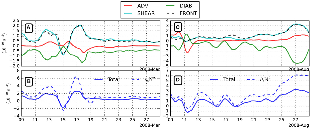
Figure 15. The advective (Ja, solid red), shear (Jf, solid light blue), diabatic (Jd, solid green) PV fluxes and Frontogenesis term (FRONT, dashed black) in March (A) and in August (C) 2008. The stratification time rate (dashed blue) and the total term (${\partial }_{\text{t}}\overline{{\text{N}}^2}+\frac{\text{bvp}{|}_{{\text{z}}_{\text{b}}}^{{\text{z}}_{\text{t}}}}{\text{h}}$, solid blue) in March (B) and in August (D).

In winter, two events of restratification and one event of destratification are observed (Figure 15B). The first restratification event occurs between March 12th and 14th. This event is associated with an increase of the river discharge and a wind relaxation after a wind burst. Frontogenesis (positive FRONT values) and weak positive advective PV fluxes (positive ADV values) then control the intensification of the stratification. Non conservative PV fluxes as a combination of shear and diabatic mixing, are mutually compensated and do not contribute to the restratification process of the water column between March 12th and 14th (Figure 15A). Destratification occurs between March 14th and 16th during a higher river discharge (around 1,000 m³ s⁻¹) period but it is mainly due to an increase of the wind stress. During this event, non conservative fluxes and frontolysis (negative FRONT values) contribute to the destratification of the water column. Following the latter event (between March the 16th and 18th), a restratification occurs again driven by frontogenesis and slightly positive non conservative fluxes; the latter fluxes are associated with the wind relaxation after the second wind burst and with a high river discharge. After the last restratification event, the stratification variations decrease (or nearly constant) leading to a homogenized water column. The homogenization of the water column happens after the generation of instabilities (Figures 12A–C) and during moderate wind events (Figure 8A). It is mostly related to upwelling-favorable winds (figure not shown) which favor the flattening of isopycnals (EAPE ~ 0) and therefore the homogenization of the water column. Similar events are also observed in summer when the river discharge remains small (around 200 m³ s⁻¹). A destratification event develops between August 10th and 12th (Figure 15C) associated with an increase of the wind stress. This process is governed by negative advective PV fluxes and a weak frontolysis. The non conservative PV fluxes are weakly positive (Figure 15D). Following this destratification, two successive restratification events (13th and 17th August) occur. During these events, frontogenesis is the major contributor since non conservative fluxes (shear and diabatic mixing) are small and negative. This weak frontogenesis occurs during wind relaxation after wind gusts. It is also related to the weak summer river discharge (~200 m³ s⁻¹). Advective (stirring) processes are then close to zero. Finally, between August 24th and the 29th, a noticeable restratification event is observed with an increase of the PV from 10⁻¹⁰ s⁻³ to more than 3 × 10⁻¹⁰ s⁻³. This increase is concomitant with a river discharge increase (from 160 to 230 m³ s⁻¹) and a weak wind stress. At that time, vertical advective PV fluxes and frontogenesis are the main sources of this restratification since non conservative fluxes are almost balanced or are weakly negative.

5. Discussion

5.1. Gironde River Plume Fronts

Our high resolution numerical simulation reveals (sub)mesoscale features in the Gironde river plume and over the continental shelf. The shape of the plume appears more complex than previously simulated (Lazure and Jegou, 1998). River plumes fronts have been explored in our simulations using the sea surface salinity gradients which characterize buoyant plumes (Vic et al., 2014; Ayouche et al., 2020). Salinity and chlorophyll fronts show similar locations in the Gironde and in the Loire river plumes. The extension of these plumes has been explored using satellite SST data (2002–2014) in previous studies (Costoya et al., 2016). The former authors showed that the locations of the Gironde and Loire river plumes fronts remain close to the coast which is similar to our findings in this study. These fronts can be pushed shoreward by wind and tides, then suppressing the ballooning of the outflow (Nof and Pichevin, 2001; Isobe, 2005; Ayouche et al., 2020). In the northward coastal current of the Gironde river plume, winds may constrain the plume near the coast both in summer and in winter. Ayouche et al. (2020) showed that in idealized simulations referring to the Gironde river plume, downwelling favorable winds pushed the plume toward the coast and this might be the case in our simulations during episodic wind regimes. The river plume can also be detected from sea surface temperature in winter (Costoya et al., 2016; Yelekçi et al., 2017) when the strong river discharge strengthens the stratification; the mixed layer is then more sensitive to air-sea fluxes. Fronts in winter remain confined over the inner shelf. Their extent is limited offshore at the 100 m isobath, as shown by remote sensing observations (Yelekçi et al., 2017). Plume fronts are less prominent in summer due the weaker river discharges.

5.2. River Plume Dynamics

Inside the river plume, the circulation is mainly in geostrophic balance as observed (Mazzini et al., 2019; Alory et al., 2021) and modeled in other buoyant plumes (Nof and Pichevin, 2001; Ou et al., 2009; Schiller et al., 2011). Locally, the circulation in the river plume is ageostrophic [R_o ~ O(1)]. This ageostrophic circulation corresponds to the strongly sheared flows near the plume front (with strong curvature). Isobe (2005) shows that in the bulge, the inertial oscillations are locally constrained by the tidal dynamics. In our simulations, such a mechanism may be at work in the near-field. The friction with the coast and its geometry induce strong negative vorticity ($\frac{{\zeta }_{\text{z}}}{\text{f}}$ < -1) in the coastal current due to strong sheared flows. This ageostrophic circulation has been highlighted in idealized simulations (Ayouche et al., 2020; Lv et al., 2020) and is reproduced in the present realistic simulations. These high Rossby number flows appear during high discharge conditions or during strong wind events. Over the continental shelf and outside the river plume, the ageostrophic circulation remains weak in winter. In summer, at the rim of eddies and in filaments, strong ageostrophic circulation is observed related to a local secondary circulation (McWilliams, 2017).

The local ageostrophic circulation and its contrast with geostrophic processes have been explored in the frontal region of the Gironde river plume. This contrast has been analyzed in terms of vertical shears and linked to the wind stress intensity. We find that wind gusts (high to moderate winds) generate ageostrophic shear in the plume after a period of time (of the order of a day) during both seasons. In contrast, when the wind stress intensity is weak the geostrophic shear predominates. We emphasize the key role of the average river discharge during weak wind events to enhance density currents and therefore their induced vertical geostrophic shear. The wind-driven and geostrophic shear processes are important in the cross-shelf circulation of a coastally trapped plume (Moffat and Lentz, 2012). The river discharge induces alongshore geostrophic currents which carry out the downcoast freshwater transport in the northern Hemisphere (Horner-Devine et al., 2015). The interaction between surface intensified river plumes and downwelling favorable winds induces geostrophic sheared flows (weak to moderate winds) in regions of strong horizontal density gradients (Spall and Thomas, 2016). In their study, high wind conditions induced circulation that prevails over the density current (Spall and Thomas, 2016). In our study, intense winds induce ageostrophic sheared currents that dominate over the density current which is similar to their key findings.

The Gironde river plume transports nutrients, sediments, and pollutants to the open ocean. Once it interacts with the open ocean, a flow barrier is formed: the plume front. This plume front is characterized by intense chlorophyll concentration and salinity/density gradients. Our study reveals also the existence of frontal ageostrophic dynamics related to winds. Such frontal dynamics and hydrology favor the concentration of phytoplankton which feeds marine organisms such as zooplankton and fish (Acha et al., 2004; Morgan et al., 2005). The concentration of nutrients and light fluctuations is sensitive to the nature of the front (convergent or divergent) and therefore influence the size of phytoplankton (Marañón et al., 2012; Marañón et al., 2015). The interactions between the frontal plume dynamics and marine biology using high resolution numerical modeling is a topic of interest for future studies to understand the biophysical dynamics in the Bay of Biscay.

5.3. Development of Instabilities in the River Plume

Energy conversion terms reveal that mixed baroclinic/barotropic instabilities, characterized by positive VBF and HRS, coexist in the near-field and the far-field of the Gironde plume. Such instabilities have a large signature over the inner-shelf (shallower than 100 m) in winter and summer.

In our realistic simulations, we have shown that the generation of such instabilities is due to the interaction between external forcings (tides and winds) and density currents in winter and mostly due to the interaction between external forcings and the surface ocean layer in summer since the river discharge is weak during this period. The combination between the Gironde discharge, tides and winds favors the development of such instabilities in the near and far fields of the plume. Our results confirm what has been shown in previous idealized simulations (Jia and Yankovsky, 2012; Ayouche et al., 2020).

Symmetric instabilities have also been investigated using the Hoskins and Richardson number criteria. These instabilities develop in different regions of the plume,the bulge and the coastal current, when the PV is negative and the Richardson number is smaller than 1. They are generated through the impact of winds on the bulge and coastal current. Symmetric instabilities in our realistic simulations remain close to the coast in winter and extend from the coast to the continental shelf in summer. These instabilities may overwhelm the water column in the bottom-attached plume interior in March and August. In August, symmetric instabilities remain near the surface locally over the continental shelf. Such instabilities have been studied previously in idealized simulations (Ayouche et al., 2020; Lv et al., 2020). In plumes frontal regions interacting with downwelling favorable winds, symmetric instabilities are triggered and restratify the plume interior (Lv et al., 2020). In idealized simulations referring to a Gironde river plume, downwelling winds trigger frontal symmetric instabilities in the coastal current of the plume and semidiurnal tides (M2) favor the generation of these instabilities in the bulge (Ayouche et al., 2020).

Vertical shear instabilities are also simulated (R_i < 0.25) near the bottom of the Gironde plume near (bulge) and far (coastal current) fields due to their interaction with steep bottom slopes and strong tidal currents. Their existence in the near field of the plume have been attributed to strong tidal horizontal currents near the bottom (MacDonald and Geyer, 2004; Kilcher and Nash, 2010).

The previous results highlight the possible coexistence of baroclinic and symmetric instabilities in the Gironde plume regions when R_i is smaller than one. Symmetric instabilities can be replaced by baroclinic instabilities when the Richardson number R_i is O(1). To investigate the relation between these instabilities, an EKE modal decomposition has been achieved in frontal regions where large Rossby numbers are observed locally. These instabilities have short growth time ranging from a few hours to a few days. In winter, they occur after moderate wind bursts, during relaxation events, with a transition from symmetric to baroclinic instability. Indeed, symmetric instabilities grow first followed by mixed instabilities and then baroclinic instabilities after different wind events. During this period, the turbulent activity is transferred from the EAPE to the EKE for each instability (baroclinic, symmetric, and mixed). This transition corroborates the classical Lorentz cycle (Lorenz, 1955). The origin of such instabilities is due to the interaction between density currents and the wind activity in the Gironde plume.

In summer, these instabilities also occur after wind events. The growth time is slightly weaker than in winter, due to low river discharge, but it keeps the same order of magnitude. These growths have been associated with three wind events. During the first event (moderate winds), symmetric instabilities grow first followed by baroclinic and then mixed instabilities. During the other two events, the wind is weak and therefore baroclinic instabilities grow first followed by symmetric and mixed instabilities. During this month, a transfer occurs from the EKE to the EAPE for each instability and this might be due to the presence of internal waves and their interactions with the Gironde plume. In our simulations, these decompositions reveal that frontal baroclinic instability exists through a transition from symmetric instabilities. The EKE decomposition indicates that mixed instabilities (symmetric and baroclinic instabilities) also exist but with a slower growth.

Baroclinic instabilities may exist during wind relaxation events or through a symmetric instability transition (Hetland, 2017; Lv et al., 2020). Following Stone (1970) classification, the presence of Richardson numbers between 0.84 and 1 locally in the plume during both simulated periods may explain the development of mixed baroclinic/symmetric instabilities. Another classification allows exploring the growth of non-geostrophic baroclinic instabilities based on the slope Burger number (Qu and Hetland, 2020). In further studies, the exploration of the slope Burger number in realistic simulations would help to detail the instability growth rate sensitivity.

5.4. Mixing in Ocean Boundary Layers

In our study, we retain non-linearities in the computation of PV fluxes since ageostrophic circulation is important at the river plume front compared with previous studies which neglected these non-linearities (Wenegrat et al., 2018). The three main sources of PV mixing at the surface of the ocean are buoyancy, thermal turbulent wind and wind-driven fluxes. These fluxes are similar in intensity during both months; this emphasizes their importance in the frontal region PV budget of the Gironde river plume. The main source of PV mixing at the surface of the ocean are buoyancy/salinity fronts since thermal wind fluxes always inject the PV during both periods. They are localized in the frontal region at the edge of the plume for both periods and at the rim of eddies and in filaments over the continental shelf in summer. Thermal turbulent wind PV fluxes are related to density currents that are enhanced during average to high river discharge periods, typically in winter. The latter results are limited to the bounding isopycnals defining the frontal region. Thermal turbulent wind PV fluxes are also enhanced during wind relaxation periods when the geostrophic shear increases, and when the ageostrophic circulation weakens (during both periods). This result has also been observed in the far field of the Chesapeake Bay plume during weak wind periods (Mazzini et al., 2019).

The wind-driven and surface buoyancy fluxes inject and extract PV from the frontal region of the river plume. In winter, these fluxes remain close to the coast. Surface buoyancy fluxes are injecting PV closer to the river mouth due to some local warming from the Gironde estuary and at the northern edge of the coastal current due to air-sea fluxes. Such injections of surface buoyancy fluxes are also observed in summer due to warmer temperature from the atmosphere and from the Gironde estuary. Extreme events can play a role in those surface buoyancy fluxes as observed during hurricanes. For example, Hurricane Irma in 2017 impacted the stability in the Amazon-Orinoco river plume by reducing the SST cooling and energizing the air-sea fluxes (Rudzin et al., 2020). Surface buoyancy fluxes are also observed over the continental shelf as patterns of positive and negative fluxes that result from the air-sea interactions and internal tides oscillations. Internal waves, due to strong semi-diurnal tidal currents (Pichon and Corréard, 2006), have been observed over the continental shelf of the Bay of Biscay in late summer and they are reproduced in our simulations.

Wind-driven fluxes are sensitive to the wind direction and intensity. They are highly variable in space and time in the frontal region of the plume. In winter, these fluxes inject PV at the inner edge of the plume front and remove potential vorticity north of the coastal current and at the offshore edge of the plume front. While in summer, injection and removal of PV vary along the front (meridional direction). Over the continental shelf, positive and negative fluxes are mainly compensated. The PV removal and injection vary depending on whether the wind is along-front or cross-front and on the induced frontal symmetric instabilities. The injection of PV by winds can be also observed during periods when the wind is weak and the geostrophic shear increases. The wind-driven removal/destruction of PV by winds has been observed in ocean fronts when the wind is downfront which induces an upward flux at the sea surface (Thomas, 2005). The latter have also been observed for weak to moderate downfront winds interacting with buoyant coastal plumes (Spall and Thomas, 2016).

Since the frontal region of the plume is interacting with the bottom most of the time in our simulation, bottom PV fluxes have been analyzed. They remain relatively weak and are not expected to contribute effectively to the PV mixing of the plume frontal region.

5.5. River Plume Interior Mixing

In the ocean interior, the mixing has been characterized by frontogenesis and PV mixing processes in the Gironde river plume frontal region. In winter, during river discharge intensification periods and/or wind relaxation events, the frontogenesis prevails and the plume interior restratification is intensified. In contrast, destratification is characterized by non conservative fluxes (diabatic and shear mixing) and frontolysis through wind intensification periods. These budgets have been evaluated in idealized simulations characterizing the Gironde river plume in a winter regime (Ayouche et al., 2020). In their study, they show that downwelling favorable winds with average discharge favor the destratification in the coastal current (far field) of the plume. The former authors also show that semi-diurnal tides generate intense fronts (frontogenesis) near the river mouth (near-field region) that restratify the plume. Conversely, in a stratified regime (summer season), weak restratification events are observed during wind relaxation due to the small river discharge. The destratification in summer is also linked to a high wind event inducing frontolysis and the growth of ageostrophic shear. Similar results have been observed in idealized simulations in stratified buoyant coastal plumes where the wind stress is linked to the reduction of PV and therefore to destratification (Spall and Thomas, 2016; Lv et al., 2020). In their study, the restratification processes are observed during wind relaxation periods when the geostrophic shear becomes dominant.

6. Conclusion

The Gironde river plume appears as a complex system under the influence of varying forcings: the river discharge, wind stress fluctuations, tide related processes. The interaction of all these nonlinear processes strongly shapes the development of instabilities and the mixing efficiency in the river plume.

Based on high resolution numerical simulations, we highlighted the buoyant frontal activity at meso- and sub-mesoscale with a contrasted seasonal activity. This buoyant frontal dynamics is linked with geostrophic (driven by river discharge) and ageostrophic (associated with wind stress) motions. The geostrophic balanced circulation exists in the river plume interior (in the near field and the coastal current) whereas the ageostrophic circulation occurs locally in the frontal regions. Exploring two seasons (winter and summer), numerical simulations indicate that ageostrophic features are more intense over the inner shelf (shallower than 100 m) in winter and extend to the whole continental shelf in summer. Our understanding of geostrophic and ageostrophic dynamics is giving insights for future observations of coastal ocean submesoscale through satellite altimetry (e.g., SWOT mission).

These nonlinear processes favor the development and coexistence of instabilities (baroclinic, frontal symmetric, and barotropic) in different regions of the river plume. We simulated these instabilities. We observed baroclinic and symmetric instabilities in frontal regions. Such instabilities are growing in a mixed mode (co-existing) or through a transition sequence between symmetric and baroclinic instabilities linked with wind events. These instabilities can also develop in the near field or the coastal current (with a signature in energy and PV fluxes). Other instabilities such as barotropic instability are also find to coexist with baroclinic and symmetric instabilities, in the near field and the coastal current due to the interaction between Gironde river plume and moderate to high wind gusts, tidal currents and river discharge growth.

The potential source of the mixing in river plumes is sustained through different processes (ocean fronts, air/sea interactions, and wind dynamics). Based on our simulations, the mixing appears mainly linked to the frontal dynamics at the edge of the river plume. The analysis of PV fluxes in the ocean interior and at the surface at small temporal (hourly fields) and spatial (400 m resolution) scales allows quantifying the mixing. PV fluxes are driven by density currents (frontogenesis), heat fluxes, internal waves and wind forcings (non conservative, i.e., shear and diabatic, mixing processes). The estimate of the PV budget relies on approximations and hypotheses (see section 2.2.2). Besides, mixing processes in the simulations are highly sensitive to model parameterizations. Therefore, future efforts should be oriented toward in situ measurements that would help us to assess or tune some model parameterizations and to test some of our hypotheses. In the near future, in situ experiments will be proposed to measure the turbulent mixing (i.e., turbulence microstructure measurements) to improve model parametrization for the river plume in tidally-driven coastal environments.

Data Availability Statement

The raw data supporting the conclusions of this article will be made available by the authors, without undue reservation.

Author Contributions

AA, GC, and XC designed the study. AA, GC, XC, and NA contributed to the writing. AA performed most of the analyses. ST develops the previous CROCO configuration used for this analysis. All authors contributed to the article and approved the submitted version.

Funding

This work has been driven with the support of Brittany region. This study is part of the COCTO project (SWOT science team program) funded by the CNES. The Ph.D. thesis of A. Ayouche was funded by Brittany region and Ifremer. Model simulations were carried out with GENCI (French National High-Performance Computing Organization) computational resources administered at the CINES (National Computing Center for Higher Education).

Conflict of Interest

The authors declare that the research was conducted in the absence of any commercial or financial relationships that could be construed as a potential conflict of interest.

Acknowledgments

The authors thank Sabine Schmidt for providing the MAGEST in situ observations. MAGEST Verdon station was part of the DIAGIR project.

References

Acha, E. M., Mianzan, H. W., Guerrero, R. A., Favero, M., and Bava, J. (2004). Marine fronts at the continental shelves of austral South America - Physical and ecological processes. J. Mar. Syst. 44, 83–105. doi: 10.1016/j.jmarsys.2003.09.005

CrossRef Full Text | Google Scholar

Akpınar, A., Charria, G., Theetten, S., and Vandermeirsch, F. (2020). Cross-shelf exchanges in the northern Bay of Biscay. J. Mar. Syst. 205:103314. doi: 10.1016/j.jmarsys.2020.103314

CrossRef Full Text | Google Scholar

Alory, G., Da-Allada, C. Y., Djakouré, S., Dadou, I., Jouanno, J., and Loemba, D. P. (2021). Coastal upwelling limitation by onshore geostrophic flow in the gulf of guinea around the Niger river plume. Front. Mar. Sci. 7:1116. doi: 10.3389/fmars.2020.607216

CrossRef Full Text | Google Scholar

Ayouche, A., Carton, X., Charria, G., Theettens, S., and Ayoub, N. (2020). Instabilities and vertical mixing in river plumes: application to the Bay of Biscay. Geophys. Astrophys. Fluid Dyn. 114, 650–689. doi: 10.1080/03091929.2020.1814275

CrossRef Full Text | Google Scholar

Chapman, D. C. (1985). Numerical treatment of cross-shelf open boundaries in a barotropic coastal ocean model. J. Phys. Oceanogr. 15, 1060–1075. doi: 10.1175/1520-0485(1985)015<1060:NTOCSO>2.0.CO;2

CrossRef Full Text | Google Scholar

Charria, G., Theetten, S., Vandermeirsch, F., Yelekçi, O., and Audiffren, N. (2017). Interannual evolution of (sub)mesoscale dynamics in the Bay of Biscay. Ocean Sci. 13, 777–797. doi: 10.5194/os-13-777-2017

CrossRef Full Text | Google Scholar

Cole, K. L., and Hetland, R. D. (2016). The effects of rotation and river discharge on net mixing in small-mouth kelvin number plumes. J. Phys. Oceanogr. 46, 1421–1436. doi: 10.1175/JPO-D-13-0271.1

CrossRef Full Text | Google Scholar

Contreras, M., Pizarro, O., Dewitte, B., Sepulveda, H. H., and Renault, L. (2019). Subsurface mesoscale eddy generation in the ocean off central Chile. J. Geophys. Res. 124, 5700–5722. doi: 10.1029/2018JC014723

CrossRef Full Text | Google Scholar

Costoya, X., Fernández-Nóvoa, D., deCastro, M., and Gómez-Gesteira, M. (2017). Loire and Gironde turbid plumes: Characterization and influence on thermohaline properties. J. Sea Res. 130, 7–16. doi: 10.1016/j.seares.2017.04.003

CrossRef Full Text | Google Scholar

Costoya, X., Fernández-Nóvoa, D., deCastro, M., Santos, F., Lazure, P., and Gómez-Gesteira, M. (2016). Modulation of sea surface temperature warming in the Bay of Biscay by Loire and Gironde rivers. J. Geophys. Res. 121, 966–979. doi: 10.1002/2015JC011157

CrossRef Full Text | Google Scholar

Debreu, L., Marchesiello, P., Penven, P., and Cambon, G. (2012). Two-way nesting in split-explicit ocean models: algorithms, implementation and validation. Ocean Model. 49–50, 1–21. doi: 10.1016/j.ocemod.2012.03.003

CrossRef Full Text | Google Scholar

Dee, D. P., Uppala, S. M., Simmons, A. J., Berrisford, P., Poli, P., Kobayashi, S., et al. (2011). The era-interim reanalysis: configuration and performance of the data assimilation system. Q. J. R. Meteorol. Soc. 137, 553–597. doi: 10.1002/qj.828

CrossRef Full Text | Google Scholar

Frouin, R., Fiúza, A. F. G., Ambar, I., and Boyd, T. J. (1990). Observations of a Poleward surface current off the coasts of Portugal and Spain during winter. J. Geophys. Res. 95, 679–691. doi: 10.1029/JC095iC01p00679

CrossRef Full Text | Google Scholar

Garcia-Soto, C., Pingree, R. D., and Valdés, L. (2002). Navidad development in the southern Bay of Biscay: Climate change and Swoddy structure from remote sensing and in situ measurements. J. Geophys. Res. 107, 28-1–28-29. doi: 10.1029/2001JC001012

CrossRef Full Text | Google Scholar

Godin, G. (1972). The Analysis of Tides. Toronto, ON; Buffalo, NY: University of Toronto Press.

Google Scholar

Graham, J. A., Rosser, J. P., O'Dea, E., and Hewitt, H. T. (2018). Resolving shelf break exchange around the European northwest shelf. Geophys. Res. Lett. 45, 12,386–12,395. doi: 10.1029/2018GL079399

CrossRef Full Text | Google Scholar

Gula, J., Molemaker, M., and Mcwilliams, J. (2016). Topographic generation of submesoscale centrifugal instability and energy dissipation. Nat. Commun. 7:12811. doi: 10.1038/ncomms12811

PubMed Abstract | CrossRef Full Text | Google Scholar

Hetland, R. (2005). Relating river plume structure to vertical mixing. J. Phys. Oceanogr. 35, 1667–1688. doi: 10.1175/JPO2774.1

CrossRef Full Text | Google Scholar

Hetland, R. D. (2010). The effects of mixing and spreading on density in near-field river plumes. Dyn. Atmos. Oceans 49, 37–53. doi: 10.1016/j.dynatmoce.2008.11.003

CrossRef Full Text | Google Scholar

Hetland, R. D. (2017). Suppression of baroclinic instabilities in buoyancy-driven flow over sloping bathymetry. J. Phys. Oceanogr. 47, 49–68. doi: 10.1175/JPO-D-15-0240.1

CrossRef Full Text | Google Scholar

Horner-Devine, A. (2009). The bulge circulation in the Columbia river plume. Contin. Shelf Res. 29, 234–251. doi: 10.1016/j.csr.2007.12.012

CrossRef Full Text | Google Scholar

Horner-Devine, A. R., Hetland, R. D., and MacDonald, D. G. (2015). Mixing and transport in coastal river plumes. Annu. Rev. Fluid Mech. 47, 569–594. doi: 10.1146/annurev-fluid-010313-141408

CrossRef Full Text | Google Scholar

Hoskins, B. J. (1974). The role of potential vorticity in symmetric stability and instability. Q. J. R. Meteorol. Soc. 100, 480–482. doi: 10.1002/qj.49710042520

CrossRef Full Text | Google Scholar

Huret, M., Bourriau, P., Doray, M., Gohin, F., and Petitgas, P. (2018). Survey timing vs. ecosystem scheduling: degree-days to underpin observed interannual variability in marine ecosystems. Prog. Oceanogr. 166, 30–40. doi: 10.1016/j.pocean.2017.07.007

CrossRef Full Text | Google Scholar

Isobe, A. (2005). Ballooning of river-plume bulge and its stabilization by tidal currents. J. Phys. Oceanogr. 35, 2337–2351. doi: 10.1175/JPO2837.1

CrossRef Full Text | Google Scholar

Jia, Y., and Yankovsky, A. (2012). The impact of ambient stratification on freshwater transport in a river plume. J. Mar. Res. 70, 69–92. doi: 10.1357/002224012800502408

CrossRef Full Text | Google Scholar

Kang, D. (2015). Energetics of eddy-mean flow interactions in the Gulf Stream region. J. Phys. Oceanogr. 45, 1103–1120. doi: 10.1175/JPO-D-14-0200.1

CrossRef Full Text | Google Scholar

Karagiorgos, J., Vervatis, V., and Sofianos, S. (2020). The impact of tides on the Bay of Biscay dynamics. J. Mar. Sci. Eng. 8:617. doi: 10.3390/jmse8080617

CrossRef Full Text | Google Scholar

Kastner, S. E., Horner-Devine, A. R., and Thomson, J. (2018). The influence of wind and waves on spreading and mixing in the Fraser river plume. J. Geophys. Res. 123, 6818–6840. doi: 10.1029/2018JC013765

CrossRef Full Text | Google Scholar

Kilcher, L. F., and Nash, J. D. (2010). Structure and dynamics of the Columbia river tidal plume front. J. Geophys. Res. 115:C05S90. doi: 10.1029/2009JC006066

CrossRef Full Text | Google Scholar

Kourafalou, V. H., Lee, T. N., Oey, L.-Y., and Wang, J. D. (1996a). The fate of river discharge on the continental shelf: 2. transport of coastal low-salinity waters under realistic wind and tidal forcing. J. Geophys. Res. 101, 3435–3455. doi: 10.1029/95JC03025

CrossRef Full Text | Google Scholar

Kourafalou, V. H., Oey, L.-Y., Wang, J. D., and Lee, T. N. (1996b). The fate of river discharge on the continental shelf: 1. modeling the river plume and the inner shelf coastal current. J. Geophys. Res. 101, 3415–3434. doi: 10.1029/95JC03024

CrossRef Full Text | Google Scholar

Koutsikopoulos, C., Beillois, P., Leroy, C., and Taillefer, F. (1998). Temporal trends and spatial structures of the sea surface temperature in the Bay of Biscay. Oceanol. Acta 21, 335–344. doi: 10.1016/S0399-1784(98)80020-0

CrossRef Full Text | Google Scholar

Lapeyre, G., Klein, P., and Hua, B. L. (2006). Oceanic restratification forced by surface frontogenesis. J. Phys. Oceanogr. 36, 1577–1590. doi: 10.1175/JPO2923.1

CrossRef Full Text | Google Scholar

Large, W. G., McWilliams, J. C., and Doney, S. C. (1994). Oceanic vertical mixing: A review and a model with a nonlocal boundary layer parameterization. Rev. Geophys. 32, 363–403. doi: 10.1029/94RG01872

CrossRef Full Text | Google Scholar

Lazure, P., Garnier, V., Dumas, F., Herry, C., and Chifflet, M. (2009). Development of a hydrodynamic model of the Bay of Biscay. Validation of hydrology. Contin. Shelf Res. 29, 985–997. doi: 10.1016/j.csr.2008.12.017

CrossRef Full Text | Google Scholar

Lazure, P., and Jegou, A.-M. (1998). 3d modelling of seasonal evolution of Loire and Gironde plumes on Biscay bay continental shelf. Oceanol. Acta 21, 165–177. doi: 10.1016/S0399-1784(98)80006-6

CrossRef Full Text | Google Scholar

Le Boyer, A., Charria, G., Cann, B., Lazure, P., and Marié, L. (2013). Circulation on the shelf and the upper slope of the Bay of Biscay. Contin. Shelf Res. 55, 97–107. doi: 10.1016/j.csr.2013.01.006

CrossRef Full Text | Google Scholar

Le Cann, B., and Serpette, A. (2009). Intense warm and saline upper ocean inflow in the Southern Bay of Biscay in Autumn-winter 2006–2007. Contin. Shelf Res. 29, 1014–1025. doi: 10.1016/j.csr.2008.11.015

CrossRef Full Text | Google Scholar

Liu, W.-C., Chen, W.-B., Cheng, R. T., and Hsu, M.-H. (2008). Modelling the impact of wind stress and river discharge on Danshuei river plume. Appl. Math. Model. 32, 1255–1280. doi: 10.1016/j.apm.2007.03.009

CrossRef Full Text | Google Scholar

Lorenz, E. N. (1955). Available potential energy and the maintenance of the general circulation. Tellus 7, 157–167. doi: 10.3402/tellusa.v7i2.8796

CrossRef Full Text | Google Scholar

Lv, R., Cheng, P., and Gan, J. (2020). Adjustment of river plume fronts during downwelling-favorable wind events. Contin. Shelf Res. 202:104143. doi: 10.1016/j.csr.2020.104143

CrossRef Full Text | Google Scholar

Lyard, F. H., Allain, D. J., Cancet, M., Carrére, L., and Picot, N. (2020). FES2014 global ocean tides atlas: design and performances. Ocean Sci. Discuss. 2020, 1–40. doi: 10.5194/os-2020-96

CrossRef Full Text | Google Scholar

MacDonald, D. G., and Geyer, W. R. (2004). Turbulent energy production and entrainment at a highly stratified estuarine front. J. Geophys. Res. 109:C05004. doi: 10.1029/2003JC002094

CrossRef Full Text | Google Scholar

Mara nón, E., Cerme no, P., Latasa, M., and Tadonléké, R. D. (2012). Temperature, resources, and phytoplankton size structure in the ocean. Limnol. Oceanogr. 57, 1266–1278. doi: 10.4319/lo.2012.57.5.1266

CrossRef Full Text | Google Scholar

Marañón, E., Cermeño, P., Latasa, M., and Tadonléké, R. D. (2015). Resource supply alone explains the variability of marine phytoplankton size structure. Limnol. Oceanogr. 60, 1848–1854. doi: 10.1002/lno.10138

CrossRef Full Text | Google Scholar

Marchesiello, P., McWilliams, J. C., and Shchepetkin, A. (2001). Open boundary conditions for long-term integration of regional oceanic models. Ocean Model. 3, 1–20. doi: 10.1016/S1463-5003(00)00013-5

CrossRef Full Text | Google Scholar

Marshall, J., Jamous, D., and Nilsson, J. (2001). Entry, flux, and exit of potential vorticity in ocean circulation. J. Phys. Oceanogr. 31, 777–789. doi: 10.1175/1520-0485(2001)031<0777:EFAEOP>2.0.CO;2

CrossRef Full Text | Google Scholar

Marshall, J. C., and Nurser, A. J. G. (1992). Fluid dynamics of oceanic thermocline ventilation. J. Phys. Oceanogr. 22, 583–595. doi: 10.1175/1520-0485(1992)022<0583:FDOOTV>2.0.CO;2

CrossRef Full Text | Google Scholar

Mazzini, P. L. F., Chant, R. J., Scully, M. E., Wilkin, J., Hunter, E. J., and Nidzieko, N. J. (2019). The impact of wind forcing on the thermal wind shear of a river plume. J. Geophys. Res. 124, 7908–7925. doi: 10.1029/2019JC015259

CrossRef Full Text | Google Scholar

McWilliams, J. C. (2017). Submesoscale surface fronts and filaments: secondary circulation, buoyancy flux, and frontogenesis. J. Fluid Mech. 823, 391–432. doi: 10.1017/jfm.2017.294

CrossRef Full Text | Google Scholar

Moffat, C., and Lentz, S. (2012). On the response of a buoyant plume to downwelling-favorable wind stress. J. Phys. Oceanogr. 42, 1083–1098. doi: 10.1175/JPO-D-11-015.1

CrossRef Full Text | Google Scholar

Morgan, C., De Robertis, A., and Zabel, R. (2005). Columbia River plume fronts. I. Hydrography, zooplankton distribution, and community composition. Mar. Ecol. Prog. Ser. 299, 19–31. doi: 10.3354/meps299019

CrossRef Full Text | Google Scholar

Nof, D., and Pichevin, T. (2001). The ballooning of outflows. J. Phys. Oceanogr. 31, 3045–3058. doi: 10.1175/1520-0485(2001)031<3045:TBOO>2.0.CO;2

CrossRef Full Text | Google Scholar

Orlanski, I. (1976). A simple boundary condition for unbounded hyperbolic flows. J. Comput. Phys. 21, 251–269. doi: 10.1016/0021-9991(76)90023-1

CrossRef Full Text | Google Scholar

Ou, S., Zhang, H., and Wang, D.-x. (2009). Dynamics of the buoyant plume off the Pearl river estuary in summer. Environ. Fluid Mech. 9, 471–492. doi: 10.1007/s10652-009-9146-3

CrossRef Full Text | Google Scholar

Pichon, A., and Corréard, S. (2006). Internal tides modelling in the Bay of Biscay: comparisons with observations. Sci. Mar. 70, 65–88. doi: 10.3989/scimar.2006.70s165

CrossRef Full Text | Google Scholar

Pingree, R., and Le Cann, B. (1989). Celtic and armorican slope and shelf residual currents. Prog. Oceanogr. 23, 303–338. doi: 10.1016/0079-6611(89)90003-7

CrossRef Full Text | Google Scholar

Pingree, R., Sinha, B., and Griffiths, C. (1999). Seasonality of the European slope current (Goban spur) and ocean margin exchange. Contin. Shelf Res. 19, 929–975. doi: 10.1016/S0278-4343(98)00116-2

CrossRef Full Text | Google Scholar

Pingree, R. D., and Le Cann, B. (1990). Structure, strength and seasonality of the slope currents in the Bay of Biscay region. J. Mar. Biol. Assoc. United Kingdom 70, 857–885. doi: 10.1017/S0025315400059117

CrossRef Full Text | Google Scholar

Piton, V., Herrmann, M., Lyard, F., Marsaleix, P., Duhaut, T., Allain, D., et al. (2020). Sensitivity study on the main tidal constituents of the gulf of Tonkin by using the frequency-domain tidal solver in t-UGOM. Geosci. Model Dev. 13, 1583–1607. doi: 10.5194/gmd-13-1583-2020

CrossRef Full Text | Google Scholar

Puillat, I., Lazure, P., Jégou, A., Lampert, L., and Miller, P. (2004). Hydrographical variability on the French continental shelf in the Bay of Biscay, during the 1990s. Contin. Shelf Res. 24, 1143–1163. doi: 10.1016/j.csr.2004.02.008

CrossRef Full Text | Google Scholar

Qu, L., and Hetland, R. (2020). Nongeostrophic baroclinic instability over sloping bathymetry: Buoyant flow regime. J. Phys. Oceanogr. 50, 1937–1956. doi: 10.1175/JPO-D-19-0145.1

CrossRef Full Text | Google Scholar

Rathan, S., and Naga Raju, G. (2018). A modified fifth-order weno scheme for hyperbolic conservation laws. Comput. Math. Appl. 75, 1531–1549. doi: 10.1016/j.camwa.2017.11.020

CrossRef Full Text | Google Scholar

Roullet, G., Capet, X., and Maze, G. (2014). Global interior eddy available potential energy diagnosed from Argo floats. Geophys. Res. Lett. 41, 1651–1656. doi: 10.1002/2013GL059004

CrossRef Full Text | Google Scholar

Rubio, A., Caballero, A., Orfila, A., Hernández-Carrasco, I., Ferrer, L., González, M., et al. (2018). Eddy-induced cross-shelf export of high CHL-a coastal waters in the se Bay of Biscay. Remote Sens. Environ. 205, 290–304. doi: 10.1016/j.rse.2017.10.037

CrossRef Full Text | Google Scholar

Rudzin, J. E., Chen, S., Sanabia, E. R., and Jayne, S. R. (2020). The air-sea response during hurricane Irma's (2017) rapid intensification over the amazon-orinoco river plume as measured by atmospheric and oceanic observations. J. Geophys. Res. 125:e2019JD032368. doi: 10.1029/2019JD032368

CrossRef Full Text | Google Scholar

Schiller, R. V., Kourafalou, V. H., Hogan, P., and Walker, N. D. (2011). The dynamics of the Mississippi river plume: Impact of topography, wind and offshore forcing on the fate of plume waters. J. Geophys. Res. 116:C06029. doi: 10.1029/2010JC006883

CrossRef Full Text | Google Scholar

Serpette, A., Cann, B., and Colas, F. (2006). Lagrangian circulation of the north Atlantic central water over the abyssal plain and continental slopes of the Bay of Biscay: description of selected mesoscale features. Sci. Mar. 70, 27–42. doi: 10.3989/scimar.2006.70s127

CrossRef Full Text | Google Scholar

Shchepetkin, A. F., and McWilliams, J. C. (2005). The regional oceanic modeling system (ROMS): a split-explicit, free-surface, topography-following-coordinate oceanic model. Ocean Model. 9, 347–404. doi: 10.1016/j.ocemod.2004.08.002

CrossRef Full Text | Google Scholar

Spall, M. A., and Thomas, L. N. (2016). Downfront winds over buoyant coastal plumes. J. Phys. Oceanogr. 46, 3139–3154. doi: 10.1175/JPO-D-16-0042.1

CrossRef Full Text | Google Scholar

Stamper, M., and Taylor, J. (2016). The transition from symmetric to Baroclinic instability in the eady model. Ocean Dyn. 67, 65–80. doi: 10.1007/s10236-016-1011-6

CrossRef Full Text | Google Scholar

Stone, P. H. (1970). On non-geostrophic Baroclinic stability: Part II. J. Atmos. Sci. 27, 721–726. doi: 10.1175/1520-0469(1970)027<0721:ONGBSP>2.0.CO;2

CrossRef Full Text | Google Scholar

Thomas, L., and Ferrari, R. (2008). Friction, frontogenesis, and the stratification of the surface mixed layer. J. Phys. Oceanogr. 38, 2501–2518. doi: 10.1175/2008JPO3797.1

CrossRef Full Text | Google Scholar

Thomas, L. N. (2005). Destruction of potential vorticity by winds. J. Phys. Oceanogr. 35, 2457–2466. doi: 10.1175/JPO2830.1

CrossRef Full Text | Google Scholar

Thomson, R. E., and Fine, I. V. (2003). Estimating mixed layer depth from oceanic profile data. J. Atmos. Ocean. Technol. 20, 319–329. doi: 10.1175/1520-0426(2003)020<0319:EMLDFO>2.0.CO;2

CrossRef Full Text | Google Scholar

Toublanc, F. T., Ayoub, N., Lyard, F., Marsaleix, P., and Allain, D. (2018). Tidal downscaling from the open ocean to the coast: a new approach applied to the Bay of Biscay. Ocean Model. 124, 16–32. doi: 10.1016/j.ocemod.2018.02.001

CrossRef Full Text | Google Scholar

Vandermeirsch, F., Charraudeau, M., Bonnat, A., Fichaut, M., Maillard, C., Gaillard, F., et al. (2010). “Bay of Biscay's temperature and salinity climatology,” in XII International Symposium on Oceanography of the Bay of Biscay (Plouzané).

Google Scholar

Vic, C., Berger, H., Tréguier, A.-M., and Couvelard, X. (2014). Dynamics of an equatorial river plume: theory and numerical experiments applied to the Congo plume case. J. Phys. Oceanogr. 44, 980–994. doi: 10.1175/JPO-D-13-0132.1

CrossRef Full Text | Google Scholar

Wenegrat, J. O., Thomas, L. N., Gula, J., and McWilliams, J. C. (2018). Effects of the submesoscale on the potential vorticity budget of ocean mode waters. J. Phys. Oceanogr. 48, 2141–2165. doi: 10.1175/JPO-D-17-0219.1

CrossRef Full Text | Google Scholar

Willmott, C. J., Robeson, S. M., and Matsuura, K. (2012). A refined index of model performance. International J. Climatol. 32, 2088–2094. doi: 10.1002/joc.2419

CrossRef Full Text | Google Scholar

Wu, T., and Wu, H. (2018). Tidal mixing sustains a bottom-trapped river plume and buoyant coastal current on an energetic continental shelf. J. Geophys. Res. 123, 8026–8051. doi: 10.1029/2018JC014105

CrossRef Full Text | Google Scholar

Xu, W., Miller, P. I., Quartly, G. D., and Pingree, R. D. (2015). Seasonality and interannual variability of the European slope current from 20years of altimeter data compared with in situ measurements. Remote Sens. Environ. 162, 196–207. doi: 10.1016/j.rse.2015.02.008

CrossRef Full Text | Google Scholar

Yankovsky, A., and Chapman, D. (1997). A simple theory for the fate of buoyant coastal discharges. J. Phys. Oceanogr. 27, 1386–1401. doi: 10.1175/1520-0485(1997)027<1386:ASTFTF>2.0.CO;2

CrossRef Full Text | Google Scholar

Yelekçi, Ö., Charria, G., Capet, X., Reverdin, G., Sudre, J., and Yahia, H. (2017). Spatial and seasonal distributions of frontal activity over the French continental shelf in the Bay of Biscay. Contin. Shelf Res. 144, 65–79. doi: 10.1016/j.csr.2017.06.015

CrossRef Full Text | Google Scholar