Using Remote Sensing and in situ Measurements for Efficient Mapping and Optimal Sampling of Coral Reefs

Coral reefs are of undeniable importance to the environment, yet little is known of them on a global scale. Assessments rely on laborious, local in-water surveys. In recent years remote sensing has been useful on larger scales for certain aspects of reef science such as benthic functional type discrimination. However, remote sensing only gives indirect information about reef condition. Only through combination of remote sensing and in situ data can we achieve coverage to understand reef condition and monitor worldwide condition. This work presents an approach to global mapping of coral reef condition that intelligently selects local, in situ measurements that refine the accuracy and resolution of global remote sensing. To this end, we apply new techniques in remote sensing analysis, probabilistic modeling for coral reef mapping, and decision theory for sample selection. Our strategy represents a fundamental change in how we study coral reefs and assess their condition on a global scale. We demonstrate feasibility and performance of our approach in a proof of concept using spaceborne remote sensing together with high-quality airborne data from the NASA Earth Venture Suborbital-2 (EVS-2) Coral Reef Airborne Laboratory (CORAL) mission as a proxy for in situ samples. Results indicate that our method is capable of extrapolating in situ features and refining information from remote sensing with increasing accuracy. Furthermore, the results confirm that decision theory is a powerful tool for sample selection.

Introduction

In addition to their significance in the marine biome, coral reefs are important to the cultural and economic lives of hundreds of millions of people around the world (Moberg and Folke, 1999; Costanza et al., 2014). It is incontrovertible that many coral reefs are in various stages of decline and may be unable to withstand the consequences of global climate change (Smith and Buddemeier, 1992; Hoegh-Guldberg et al., 2007, 2017; Pandolfi et al., 2011; Gattuso et al., 2015). Yet a small fraction of the world’s reef area has been studied quantitatively (i.e., 0.01–0.1%) as most reef assessments largely rely on local in-water surveys (Hochberg and Atkinson, 2003). Therefore, our current understanding may not be representative of the reef under study, nor the regional and global reef ecosystem given existing data constraints (Hochberg and Gierach, 2021).

Remote sensing from airborne and spaceborne platforms have proven to be a useful tool for aspects of reef science (Hedley et al., 2016). Early applications of remote sensing to coral reef environments focused on mapping reef geomorphology and ecological zonation (Kuchler et al., 1988; Green et al., 1996; Mumby et al., 2004). In the past few decades, much of remote sensing has focused on mapping habitats using qualitative descriptors comprising various combinations of substrate (e.g., sand, limestone, rubble), benthic functional type (e.g., coral, algae, seagrass), reef type (e.g., fringing, patch, barrier), and/or location within the reef system (e.g., slope, flat) (Hedley et al., 2016). The recent NASA Earth Venture Suborbital-2 (EVS-2) COral Reef Airborne Laboratory (CORAL) mission focused on reef benthic functional type discrimination (Hochberg and Gierach, 2021). CORAL remote spectroscopic mapping was shown to be informative but lacked global and temporal coverage. Moreover, current remote sensing methods give only indirect information about reef condition, making in situ data critical.

Only through combination of remote sensing and in situ data can we achieve complete coverage of remote areas while capturing relevant features of reef condition to monitor worldwide change. For instance, high-quality seafloor mapping has been achieved through the collection of in situ hyperspectral measurements and stereo imagery (Bongiorno et al., 2018), but only at local scales through dense sampling. Information from remote sensing data can be a powerful tool for extrapolation and wide-scale coverage. Candela et al. (2020) efficiently combine spaceborne and in situ infrared spectroscopy for geologic mapping. Fossum et al. (2020) use remote sea-surface temperature images to infer spatial patterns in the evolution of oceanographic conditions. Other approaches combine remote bathymetry with in situ imagery for benthic habitat mapping (Rao et al., 2017; Shields et al., 2020).

Furthermore, we seek to improve global mapping of coral reef condition by intelligently selecting sparse, in situ measurements. Specifically, samples that refine the accuracy and resolution of global remote sensing by adapting to the current state of knowledge of the environment. Currently most works regarding adaptive sampling for marine surveys fail to exploit the power of remote sensing; consequently, they only map simple quantities such as salinity, temperature, altimetry, or dissolved oxygen measurements (Binney et al., 2010; Flaspohler et al., 2019; Stankiewicz et al., 2021). Rao et al. (2017) use a deep learning architecture that does not allow for adaptive sampling. Shields et al. (2020) use a somewhat similar approach, but they have recently taken some first steps toward enabling adaptive sampling through numerical approximations. Fossum et al. (2020) present a framework with potential, but it has yet to be used for adaptive sampling. Candela et al. (2020) present an adaptive sampling method that has been tested in simulations and the field, although focused on geologic applications.

The motivation of this work is to enable global mapping and optimal sampling of coral reefs. To this end, we apply new techniques in orbital data analysis, probabilistic modeling for mapping, and decision theory for sample selection. We apply machine learning to interpretation of imaging spectroscopy data from the CORAL mission to extract features related to physical properties of the underwater environment indicative of coral condition. We also develop automatic mission and path planning that could be executed by human divers or autonomous underwater vehicles to refine and validate the coral geographical map. Our strategy represents a fundamental change in how we understand coral reefs and assess their condition. Instead of small, infrequent, uncorrelated studies of isolated locations, we begin to measure coral reefs globally, updating often, and seeing worldwide patterns. The methodology and results presented have direct applicability and benefit to future NASA imaging spectroscopic missions, including the Surface Biology and Geology Designated Observable (National Academies of Sciences, Engineering, and Medicine (NASEM)., 2018).

Materials and Methods

We start by portraying the data products we utilize in this study. We then explain our probabilistic machine learning model for coral reef mapping. Finally, we review various state-of-the-art strategies that quantify and leverage the information contained in our probabilistic model to enable intelligent sample selection.

Remote Sensing Data

Here we use the term “remote sensing” to refer to spaceborne or airborne sensors; we do not consider in-water remote sensing methods. We use high-resolution airborne data from the CORAL mission as a proxy for in situ measurements. CORAL mapped portions of the Great Barrier Reef, main Hawaiian Islands, Marianas Islands, and Palau in 2016–2017. Herein we analyze two flight lines from Heron Island, Australia on 17 September 2016 and Kaneohe Bay in Oahu, Hawaii on 6 March 2017 (Figure 1). Data is from the NASA/JPL Portable Remote Imaging SpectroMeter (PRISM) flown on the Tempus Applied Solutions Gulfstream-IV at 8.5 km altitude. PRISM provided water-leaving reflectance from 350 to 1050 nm (246 bands) at approximately 3 nm spectral resolution and approximately 8 m spatial resolution from which benthic reflectance and benthic functional type were derived. The benthic reflectance calculation used the shallow-water reflectance described by Maritorena et al. (1994). It was modeled using a linear non-negative combination of a set of one or more basis endmembers from a library of bottom reflectances (see Thompson et al., 2017 for more details). Here we evaluate benthic reflectance products since they provide invariance to water column properties. These products have a 420–680 nm spectral range and consist of 92 bands.

FIGURE 1

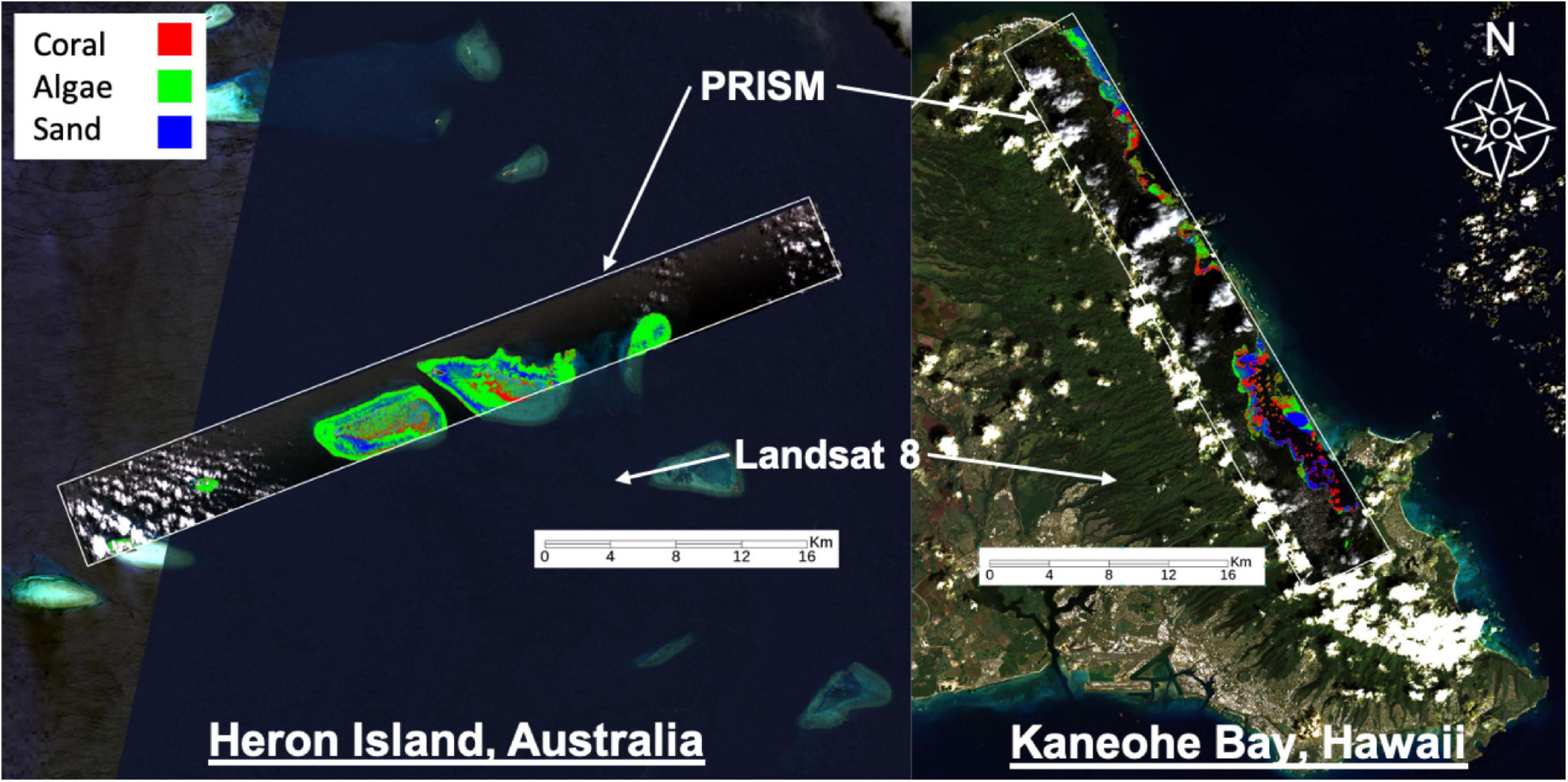
Figure 1. Remote sensing data used for this study. Landsat 8 data provides global-scale coverage but at coarse spatial and spectral resolutions that are often insufficient for benthic cover analysis. PRISM is an airborne imaging spectrometer with finer spatial and spectral resolution that was used by the CORAL mission to discriminate benthic functional types. The CORAL mission focused on three benthic functional types – coral, algae, and sand – and thus only these three types are considered herein (as shown). Coral (red), algae (green), and sand (blue) abundance maps were estimated by Thompson et al. (2017) and validated by the CORAL mission with photomosaics collected in the field.

Benthic functional type corresponds to probabilities associated with coral, algae, and sand for each seafloor pixel, and was determined by logistic regression using mean reflectance spectra from an existing spectral library (Hochberg and Atkinson, 2003; Hochberg et al., 2003). We acknowledge that additional benthic functional types could be distinguished from the PRISM dataset with utilization of other spectral libraries, but the focus of CORAL – and thus this work – was on coral, algae, and sand. Examples of PRISM-derived benthic composition from the CORAL mission are shown in Figure 1, with each pixel representing the primary benthic functional type (i.e., greatest percentage of one type per pixel, wherein all types sum to one per pixel). Herein we evaluate PRISM-derived benthic reflectance since it provides invariance to water column properties. Utilization of in situ measurements of benthic reflectance are preferred; however, there were no coincident collections of such measurements with overflights under cloud-free conditions. Maps of PRISM-derived benthic composition (i.e., coral, algae, and sand) are used to validate our mapping/sampling results, serving as “ground truth.” Note that PRISM-derived products were validated by an extensive field collection as part of the CORAL mission and is not the focus herein (e.g., Thompson et al., 2017). For example, PRISM-derived benthic composition maps were validated by 10 m × 10 m photomosaics collected in the field at random. In each 10 m × 10 m plot approximately 500–1000 digital photographs were taken, mosaicked using structure-from-motion techniques (Agisoft Metashape) to provide a single orthomosaic, and then analyzed using coral reef science standard point-count methods to provide proportional benthic composition for benthic functional types.

We also use Level 2 surface reflectance products from the orbital instrument Landsat-8 (Figure 1). Landsat-8 provides global-scale coverage, but at coarser spatial (30 m) and spectral resolution, serving as our source of remote data. We use the first four bands, which provide limited information in the visible wavelengths as compared to PRISM data. For Kaneohe Bay, we use image LC08_L2SP_064045_20170306_20200905_02_T1, which was collected on the same day as the corresponding CORAL flight line (6 March 2017). For Heron Island, we use image LC08_L2SP_091076_20161026_20200905_02_T1; due to cloud coverage issues, we had to use an image that was collected on a different day (26 October 2016).

Probabilistic Machine Learning for Coral Reef Mapping

This work adapts and extends the method by Candela et al. (2020), which combines remote sensing and in situ data for wide-area geologic mapping, to coral reefs. Here our focus is to construct benthic cover maps.

Problem Formulation

Each material reflects, emits, or absorbs light in unique ways throughout the electromagnetic spectrum. The measured signals are called spectra and contain recognizable features or patterns that can be used for composition analysis. The CORAL mission focused on coral, algae, and sand as the most common, widespread, and important types of benthic cover. We preserve that taxonomy in this study for simplicity. Figure 2 shows benthic functional type derived from spectra of coral, algae, and sand collected by PRISM during the CORAL mission.

FIGURE 2

Figure 2. Benthic reflectance of coral (left), algae (center), and sand (right) as estimated using the approach by Thompson et al. (2017) applied to PRISM data.

In this paper, we develop a method for mapping the abundances of different endmembers in a coral reef over a large area. We combine two different types of spectral measurements: low-resolution (or multispectral) remote data $\overrightarrow{x}\in X\subset {ℝ}^m$, and high-resolution (or hyperspectral) in situ data $\overrightarrow{y}\in Y\subset {ℝ}^n$. Remote spectra are available beforehand for many spatial locations $\overrightarrow{l}\in L\subset {ℝ}^2$ (latitude and longitude), but in general their spectral resolution does not permit endmember identification. In contrast, in situ spectra tend to have a spectral resolution that is sufficient for composition analysis, but unfortunately only a scarce number of samples can be collected by an agent such as a scuba diver or an AUV. Our objective is not only to extrapolate in situ samples over large areas with the assistance of remote sensing, but also to build coral reef maps that can easily adapt and improve with new information. We refer to this problem as active coral reef mapping; an illustration is shown in Figure 3.

FIGURE 3

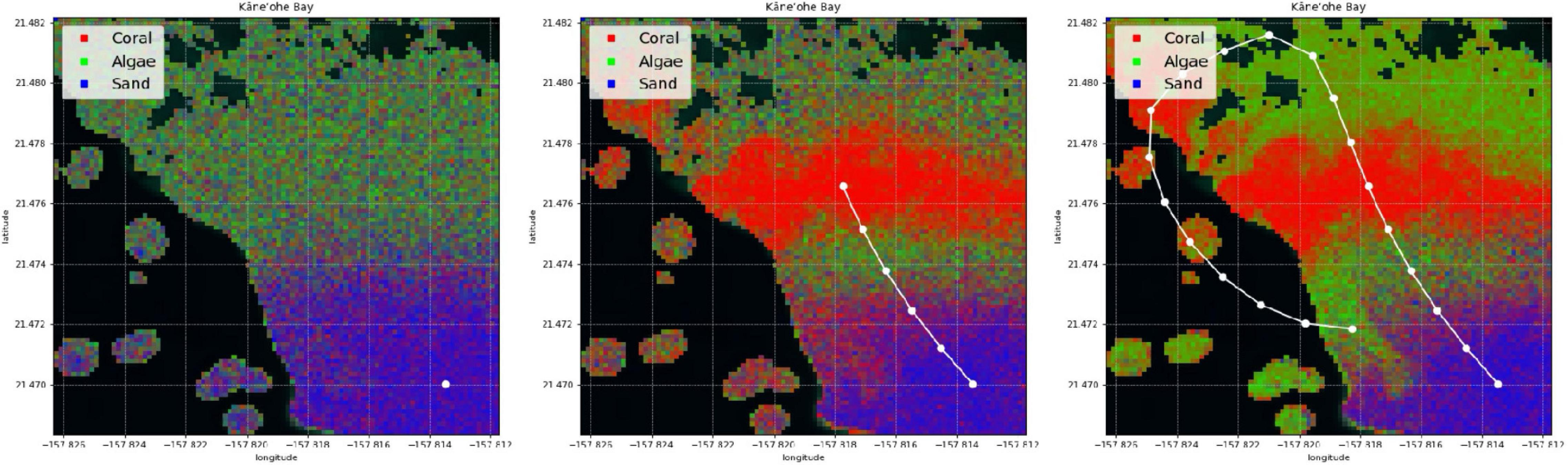
Figure 3. Example of our active process for coral reef mapping applied in Kaneohe Bay, Hawaii. The CORAL mission focused on shallow water areas, and thus a mask (as shown in black areas) is applied for depths greater than 5 m within the subsetted scenes. Experience with the CORAL data suggests that the accuracy of the standard coral, algae, and sand estimation degrades below 5 m depth. For the purposes of this paper, we focus on shallow water areas with plenty of signal. The mapping process starts with poor predictions (left). Just a few in situ samples are extrapolated throughout large areas with the assistance of remote sensing (center). The predicted coral reef map improves as more samples are collected (right).

Overall, our approach consists of two steps: spectral mapping and endmember mapping. First, we use remote sensing as a prior to extrapolate high-resolution in situ spectral measurements over large areas (Figure 4). Then, we utilize the predicted high-resolution spectra to estimate endmember abundance via spectral unmixing. We decouple these steps to allow for alternative spectral unmixing techniques. Specifically, both spectral and endmember mapping are achieved by combining different probabilistic machine learning algorithms. Gaussian process (GP) regression has been widely used in spatial statistics (Cressie, 1993; Rasmussen and Williams, 2006), adaptive sampling (Krause et al., 2008), and autonomous robotic exploration (Thompson, 2008; Kumar et al., 2019). However, most work regarding GPs (especially for AUVs) involves mapping scalar fields such as salinity, temperature, altimetry, or dissolved oxygen measurements (Binney et al., 2010; Flaspohler et al., 2019; Stankiewicz et al., 2021). In contrast, our goal is to learn and map non-scalar data, i.e., high-resolution spectra. We tackle this problem with feature extraction techniques, which reduce the dimensionality of spectra by deriving a subset of non-redundant features. Feature extraction approaches have been used for (non-scalar) benthic habitat mapping (Rao et al., 2017; Shields et al., 2020). Nonetheless, they use deep learning architectures instead of GPs for spatial modeling, thus complicating the implementation of true adaptive sampling for real time applications. Once our model predicts spectra from features, we utilize learning-based spectral unmixing algorithms to estimate endmember abundances from spectra. Figure 5 shows a summary diagram of our approach. The rest of this section describes spectral feature extraction, Gaussian process regression, and learning-based spectral unmixing in more detail.

FIGURE 4

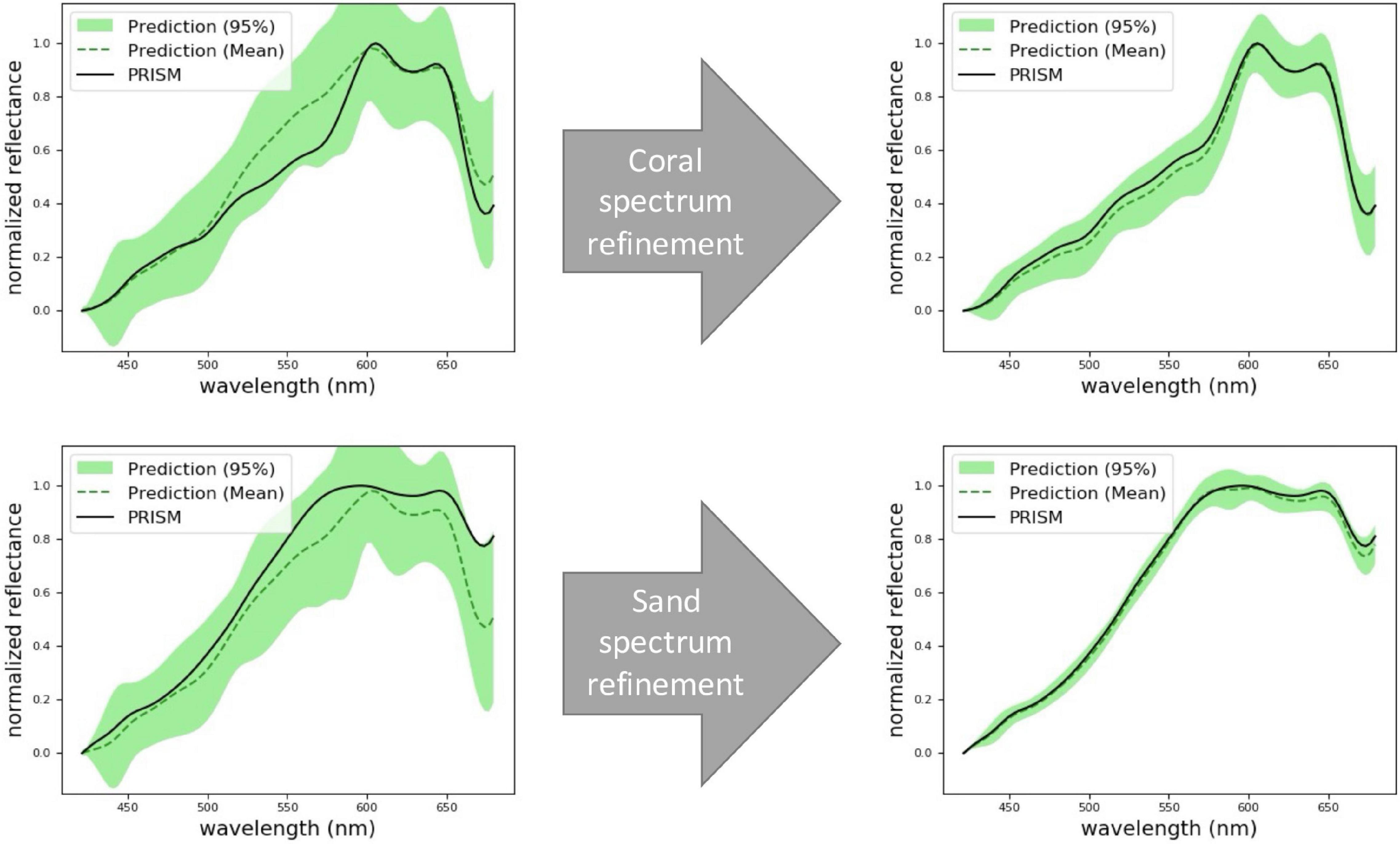
Figure 4. Prediction of coral (top row) and sand (bottom row) spectra at two locations that are never actually sampled. Here we use PRISM as the ground truth. At first, the model’s predictions have a low accuracy and a high uncertainty (left column). After collecting more samples, the model refines its spectral predictions (right column).

FIGURE 5

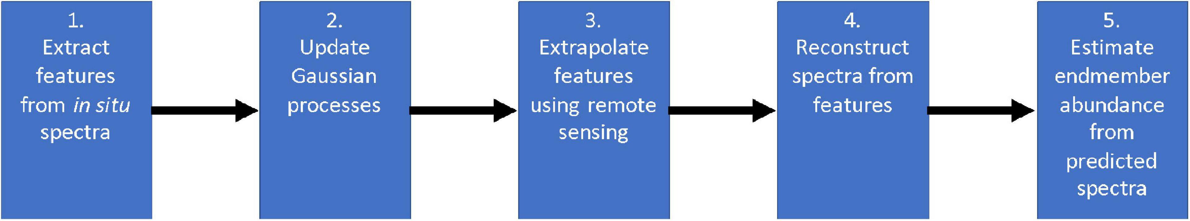
Figure 5. Active coral reef mapping process.

Extraction of Spectral Features

Many channels and wavelengths in hyperspectral measurements are strongly correlated, especially adjacent bands. This allows for dimensionality reduction techniques that learn a set of representative features that efficiently compress and capture most of the information in spectra. Hence, dimensionality reduction is also known as feature extraction. Formally, they convert a set of high-resolution observations $\overrightarrow{y}\in Y\subset {ℝ}^n$ into a set of lower dimensional features $\overrightarrow{z}\in Z\subset {ℝ}^d$, where d≪n. In this work we apply and compare two feature extraction methods: Principal Component Analysis (PCA) and the Variational Autoencoder (VAE).

Principal component analysis is a linear dimensionality reduction method that produces a sequence of orthogonal vectors, known as components, that best fit the data. Components allow individual dimensions to be linearly uncorrelated and enable the linear projection of data to a lower dimensional space. The first feature of the lower dimensional space is the one that learns most of the useful information. The next features monotonically capture less information and more noise, until the last features essentially learns pure noise.

Variational autoencoder (Kingma et al., 2013) is a neural network that performs non-linear dimensionality reduction. It produces a feature representation that resembles a standard multivariate normal distribution, i.e., $\overrightarrow{z}\sim N(\overrightarrow{0},I_d)$. This operation effectively decorrelates and normalizes features. Moreover, VAEs tend to spread information evenly across the latent dimensions while filtering noise. The VAE is composed of two networks: an encoder that extracts the features, and a decoder that reconstructs high-resolution observations using the learned features. In this work, we use the architecture described in Candela et al. (2018).

We stress that both PCA and VAE are unsupervised methods since they learn features without the need of labeled data. They offer a significant advantage over approaches that rely on manually engineered features, which tend to be domain-specific, arbitrary, and laborious.

It is worth noting that automated feature extraction requires the exact same input size. Nonetheless, it is possible to generalize and scale these algorithms to data from similar spectrometers via resampling or interpolation. This idea has been used in a similar study by Candela et al. (2020), where infrared spectra (2000–2500 nm) is used for mineral identification. First, a VAE is pretrained using data from the Airborne Visible InfraRed Imaging Spectrometer Next Generation (AVIRIS-NG), which has approximately 90 bands in the 2000–25000 nm spectral range. This VAE is then used to process resampled spectra from an Analytical Spectral Devices (ASD) FieldSpec spectrometer, which has about 400 bands in a similar spectral range. However, a substantial difference in spectral resolution or spectral range (e.g., visible vs. thermal infrared wavelengths) would most likely require a retraining process.

It is important to underscore that in our method, feature extraction ignores spatial information and neighboring context; it only considers individual spectra. It is worth noting that the recent Location Guided Autoencoder (LGA) by Yamada et al. (2021) considers spatial autocorrelations by making a simple modification to regular VAEs, potentially improving performance. For generalization purposes, we assume that spectral features are learned from spectral libraries that may not necessarily contain the corresponding spatial information. We next explain how our approach models and learns spatial autocorrelation between spectra in an adaptive manner using GPs.

Spatial Regression of Spectral Features

We use GPs for spatial regression, that is, to learn the spatial distribution of spectra throughout the scene. GPs are a powerful technique for extrapolation, as well as for the refinement of mapping as new data is collected.

Gaussian process are typically used for mapping scalar values, for example ocean temperature, salinity, altimetry, or dissolved oxygen measurements (Binney et al., 2010; Flaspohler et al., 2019; Stankiewicz et al., 2021). However, our coral reef mapping problem involves multivariate data (i.e., high-resolution spectra). We overcome this challenge by using GP regression to learn the distribution of low-dimensional features Z instead. Moreover, dimensionality reduction with either PCA or VAE uncorrelates the learned feature representation. This trick simplifies the problem substantially by allowing for the utilization of a small number of i = 1, 2,…,d independent GPs.

We next provide a brief explanation regarding the elements of our specific GP regression model. If needed, extensive GP documentation can be found in Rasmussen and Williams (2006). Formally, we define an input vector that concatenates spatial coordinates and remote spectra as $\overrightarrow{v}=[\overrightarrow{l},\overrightarrow{x}]\in V\subset {ℝ}^{2+m}$, similarly as Thompson (2008). We assume there exists a latent function fⁱ:V→ℝ that maps an input $\overrightarrow{v}$ to each feature zⁱ:

$$z^i=f^i(\overrightarrow{v})+{\in }^i.$$

In other words, the goal of a GP is to learn a distribution over the values that $f^i(\overrightarrow{v})$ can take in order to predict a spectral feature zⁱ for many locations over large areas. A GP assumes that for any set of inputs, the vector of outputs is distributed as a multivariate Gaussian, which is parametrized as follows:

$$\left[\begin{array}{c}{z}_1^{i*}\hfill \\ \mathrm{⋮}\hfill \\ z_q^{i*}\hfill \\ f^i(\overrightarrow{v_1})\hfill \\ \mathrm{⋮}\hfill \\ f^i(\overrightarrow{v_p})\hfill \end{array}\right]\sim$$

$$N(\left[\begin{array}{c}\hfill {\mathrm{\mu }}^i(\overrightarrow{v_1^{*}})\hfill \\ \hfill \mathrm{⋮}\hfill \\ \hfill {\mathrm{\mu }}^i(\overrightarrow{v_q^{*}})\hfill \\ \hfill {\mathrm{\mu }}^i(\overrightarrow{v_1})\hfill \\ \hfill \mathrm{⋮}\hfill \\ \hfill {\mathrm{\mu }}^i(\overrightarrow{v_p})\hfill \end{array}\right],[\begin{array}{c}\hfill K_{00}^i+{({\mathrm{\sigma }}_{noise}^i)}^{2}I\hfill \\ \hfill K_{UO}^i\hfill \end{array}\hspace{1em}\begin{array}{c}\hfill K_{OU}^i\hfill \\ \hfill K_{UU}^i+{({\mathrm{\sigma }}_{noise}^i)}^{2}I\hfill \end{array}]).$$

A GP combines observed (or training) data $0=\{({\overrightarrow{v}}_1^{*},z_1^{i*}),\mathrm{\dots },({\overrightarrow{v}}_q^{*},z_q^{i*})\}$ with a finite set of unseen points $U=\{(\overrightarrow{v_1},f^i({\overrightarrow{v}}_1)),\mathrm{\dots },({\overrightarrow{v}}_p,f^i(\overrightarrow{\mathit{v}}))\}$. This allows observed data to be used to predict unseen data. The prediction also follows a Gaussian distribution:

$$\left[\begin{array}{c}\hfill f^i({\overrightarrow{v}}_1)\hfill \\ \hfill \mathrm{\dots }\hfill \\ \hfill f^i({\overrightarrow{v}}_p)\hfill \end{array}\right]\sim N({\widehat{\mathrm{\mu }}}^i(U|O),{\widehat{\mathrm{\Sigma }}}^i(U|O))$$

where ${\widehat{\mathrm{\mu }}}^i$ is the predicted or posterior mean, and ${\widehat{\mathrm{\Sigma }}}^i$ is the predicted or posterior covariance matrix. These are computed using the standard formulas for conditional multivariate Gaussians (Eaton, 1983):

$${\widehat{\mathrm{\mu }}}^i(U|O)=\left[\begin{array}{c}\hfill {\mathrm{\mu }}^i({\overrightarrow{v}}_1)\hfill \\ \hfill .\hfill \\ \hfill .\hfill \\ \hfill .\hfill \\ \hfill {\mathrm{\mu }}^i({\overrightarrow{v}}_p)\hfill \end{array}\right]+K_{UO}^i{(K_{oo}^i+{({\mathrm{\sigma }}_{noise}^i)}^{2}I)}^{-1}$$

$$\left[\begin{array}{c}\hfill z_1^{i*}-{\mathrm{\mu }}^i({\overrightarrow{v}}_1^{*})\hfill \\ \hfill .\hfill \\ \hfill .\hfill \\ \hfill .\hfill \\ \hfill z_1^{i*}-{\mathrm{\mu }}^i({\overrightarrow{v}}_q^{*})\hfill \end{array}\right],$$

$${\widehat{\mathrm{\Sigma }}}^i(U|O)=K_{UU}^i+{({\mathrm{\sigma }}_{noise}^i)}^{2}I+K_{UO}^i{(K_{OO}^i+{({\mathrm{\sigma }}_{noise}^i)}^{2}I)}^{-1}{K}_{OU}^i.$$

When using GPs, one most specify a prior mean function μⁱ:V→ℝ, as well as a covariance function kⁱ:V×V→ℝ. The covariance function kⁱ is used to construct covariance matrices kⁱ, for instance:

$$K_{OU}^i=\left[\begin{array}{ccccc}\hfill k^i(\overrightarrow{v_1^{*}},\overrightarrow{\underset{1}{\mathit{v}}})\hfill & \hfill .\hfill & \hfill .\hfill & \hfill .\hfill & \hfill k^i(\overrightarrow{v_1^{*}},\overrightarrow{\underset{p}{\mathit{v}}})\hfill \\ \hfill .\hfill & \hfill .\hfill & & & \hfill .\hfill \\ \hfill .\hfill & & \hfill .\hfill & & \hfill .\hfill \\ \hfill .\hfill & & & \hfill .\hfill & \hfill .\hfill \\ \hfill k^i(\overrightarrow{v_q^{*}},\overrightarrow{\underset{1}{\mathit{v}}})\hfill & \hfill .\hfill & \hfill .\hfill & \hfill .\hfill & \hfill k^i(\overrightarrow{v_q^{*}},\overrightarrow{\underset{p}{\mathit{v}}})\hfill \end{array}\right]$$

Here we assume that the mean function is always zero (i.e.,${\mathrm{\mu }}^i(\overrightarrow{\mathit{v}})=0,\forall \overrightarrow{v}\in V$) because of the way features are normalized by both PCA and VAE. For the covariance function, we rely on the widely used squared exponential kernel. Specifically, we use a kernel that distinguishes between spatial and spectral dimensions as follows:

$$k^i(\overrightarrow{v},\overrightarrow{v}{}^{\prime })={\mathrm{\theta }}_0^i\exp (-\frac{{||\overrightarrow{l}-\overrightarrow{l{}^{\prime }}||}_2^2}{2({\mathrm{\theta }}_l^i)}-\frac{{||\overrightarrow{x}-\overrightarrow{x{}^{\prime }}||}_2^2}{2({\mathrm{\theta }}_x^i)})$$

where $[{\mathrm{\theta }}_0^i,{\mathrm{\theta }}_l^i,{\mathrm{\theta }}_x^i]$ are the kernel hyperparameters. Additionally, we utilize the GP variant for noisy observations, and thus use an additional hyperparameter for the noise standard deviation ${\sigma }_{noise}^i$ The hyperparameters $[{\mathrm{\theta }}_0^i,{\mathrm{\theta }}_l^i,{\mathrm{\theta }}_x^i,{\mathrm{\sigma }}_{noise}^i]$ are learned using the process in Rasmussen and Williams (2006).

Learning-Based Spectral Unmixing

Spectral unmixing is a procedure by which a measured spectrum is decomposed into a collection of constituent endmembers. The main characteristic of this procedure is that it estimates the proportions or abundances for at least K ≥ 2 components in each spectrum (e.g., 40% coral, 30% algae, and 30% sand in one pixel). Spectral unmixing is especially useful for scenarios in which components are highly mixed; as opposed to conventional classification, which assumes that one endmember is strongly dominant over the rest. Let us denote these endmembers’ spectra as $\overrightarrow{e_1},\overrightarrow{e_2},\mathrm{\dots },\overrightarrow{e_k}\in Y$, and their respective fractional abundances, or mixing ratios, as $\overrightarrow{r}=[r_1,r_1,\mathrm{\dots },r_k]$, such that:

$$\sum _{j=1}^K{r}_j=1,r_j\in [0,1]$$

In general, there are two different models for spectral unmixing: linear and non-linear (Lein, 2012). We explore and compare both in this work. Linear models assume that a spectrum $\overrightarrow{y}$ can be represented as a linear combination of its endmembers:

$$\overrightarrow{y}=E\overrightarrow{r},$$

where $E=[{\overrightarrow{e}}_1,{\overrightarrow{e}}_2,\mathrm{\dots }{\overrightarrow{e}}_k]$ corresponds to the endmember matrix and $\overrightarrow{r}$ is the variable to solve in the previous linear equation. We compare three different linear models:

• Unconstrained least squares (ULS): solves the equation for $\overrightarrow{r}$ using normal least squares without any constraints.

• Non-negative least squares (NNLS): solves the equation for $\overrightarrow{r}$ withr_j≥0∀r_j.

• Fully constrained least squared (FCLS): solves the equation for $\overrightarrow{r}$ with ${\sum }_{j=1}^K{r}_j=1,r_j\in [0,1]$ using the method by Heinz and Chang (2001).

Non-linear models use more complex and varied functions. Here we focus on a learning-based method for spectral unmixing. In particular, a neural network (NN) that learns how to predict fractional abundances from spectra:

$$\overrightarrow{r}=N{N}_w(\overrightarrow{y})$$

where NN is the spectral unmixing function learned by the neural network with hyperparameters or weights w. We train this network using a data set that consists of pairs of high-resolution PRISM spectra $\overrightarrow{y}$ and their associated ground-truth fractional abundances $\stackrel{\to *}{r}$. For purposes of this work, we assume that ground truth values are given by the PRISM-derived products that were generated by Thompson et al. (2017) (see Section “Remote Sensing Data”).

The neural network we use is a multilayer perceptron. For reproducibility purposes, we next explain the used architecture. The network is implemented in the deep learning framework Keras (Chollet, 2015). The size of the input layer isdim⁡(Y) = n. The output of the network consists of a softmax layer of size 3 that ensures both constraints are not violated, i.e., that it always predicts non-negative fractional abundances that sum to 1. We use the popular Adam optimizer (Kingma and Ba, 2014). The detailed architecture of the network is shown in Table 1.

TABLE 1

Table 1. Architecture of the multilayer perceptron network for spectral unmixing.

We use the Kullback–Leibler divergence (KLD) as the loss function. The Kullback–Leibler divergence is a more suitable score for mixtures of endmembers when compared to conventional classification accuracy. Regular classification assumes that mixtures are negligible. In contrast, the Kullback–Leibler divergence measures the difference between two probability distributions (Cover and Thomas, 2006). We treat the real $\stackrel{\to *}{r}$ and predicted $\overrightarrow{r}$ mixing ratios as probability distributions, which is a valid assumption since mixing ratios are non-negative and sum to 1. Hence, we use the Kullback–Leibler divergence as a loss function that measures unmixing accuracy. It is defined as follows:

$$KLD(\stackrel{\to *}{\mathit{r}}||\overrightarrow{\mathit{r}})=\sum _{j=1}^K{r}_j^{*}\log \frac{r_j^{*}}{r_j},$$

Decision Theory for Sample Selection

The agent executing the coral reef mapping mission aims to collect the most informative in situ samples. Quantitatively speaking, these are the samples that better explain and reconstruct the explored coral reef. In general, we can formulate this notion in terms of the following optimization problem:

$$\begin{array}{c}\hfill \underset{p}{\max } Info(M|P)subject toCost(P)\le Budget,\hfill \end{array}$$

where $M=\{\overrightarrow{v_1},\overrightarrow{v_2},\mathrm{\dots },\overrightarrow{v_p}\}$ is the set of pixels in the model that are to be extrapolated from remote sensing data, and $P=\{\overrightarrow{S_1},\overrightarrow{S_1},\mathrm{\dots },\overrightarrow{S_q},\}$ is the set of in situ samples$\overrightarrow{s}=[\overrightarrow{l},\overrightarrow{y}]$, given by pairs of spatial coordinates and high-resolution spectra. Here we assume there is a much larger number of pixels in the remote data than number of in situ samples, i.e.,p≫q. Info(M|P) is the information of the model given a set of in situ samples. We also include a sampling budget that can represent a quantity such as a maximum number of samples, a time constraint, etc.

In order to quantify and optimize the information of the model Info(M|P), we rely on principles of information theory and statistical learning, as well as on various algorithms for optimal sample selection. We describe and later compare four different strategies (Figure 6): random sampling, Bayesian experimental design, Monte Carlo Tree Search, and ergodic optimal control.

FIGURE 6

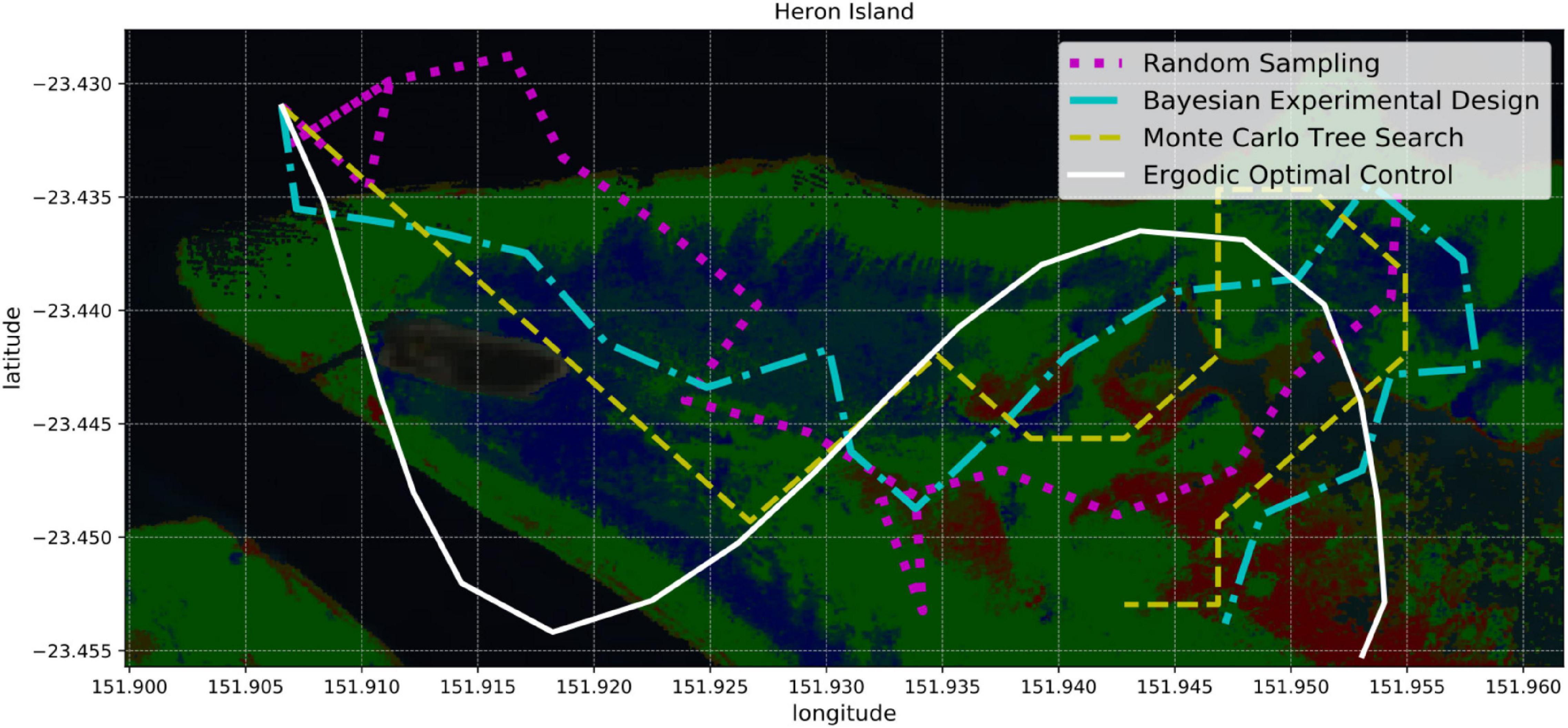
Figure 6. Four sampling strategies for coral reef mapping: random sampling, Bayesian experimental design, Monte Carlo tree search, and ergodic optimal control. Random sampling is the simplest approach since it ignores how useful future samples might be. Bayesian experimental design provides a probabilistic framework for identifying the most informative samples and planning paths accordingly. Monte Carlo tree search combines random sampling with a tree search that focuses on the most promising actions. Ergodic optimal control not only selects informative samples, but also generates smooth trajectories that can be suitable for boats or AUVs.

Random Sampling

Random sampling serves as a baseline that does not quantify nor use information from the model whatsoever, hence poorer performance is to be expected. In order to generate trajectories that are somewhat smooth, random sampling occurs inside a fixed radius at each step. We employ two different random strategies. One samples from a uniform distribution inside the circular region, and one samples from a uniform distribution along the perimeter of the region. Figure 7 shows an illustration of both random sampling methods, which we call random uniform (RU) and random edge (RE).

FIGURE 7

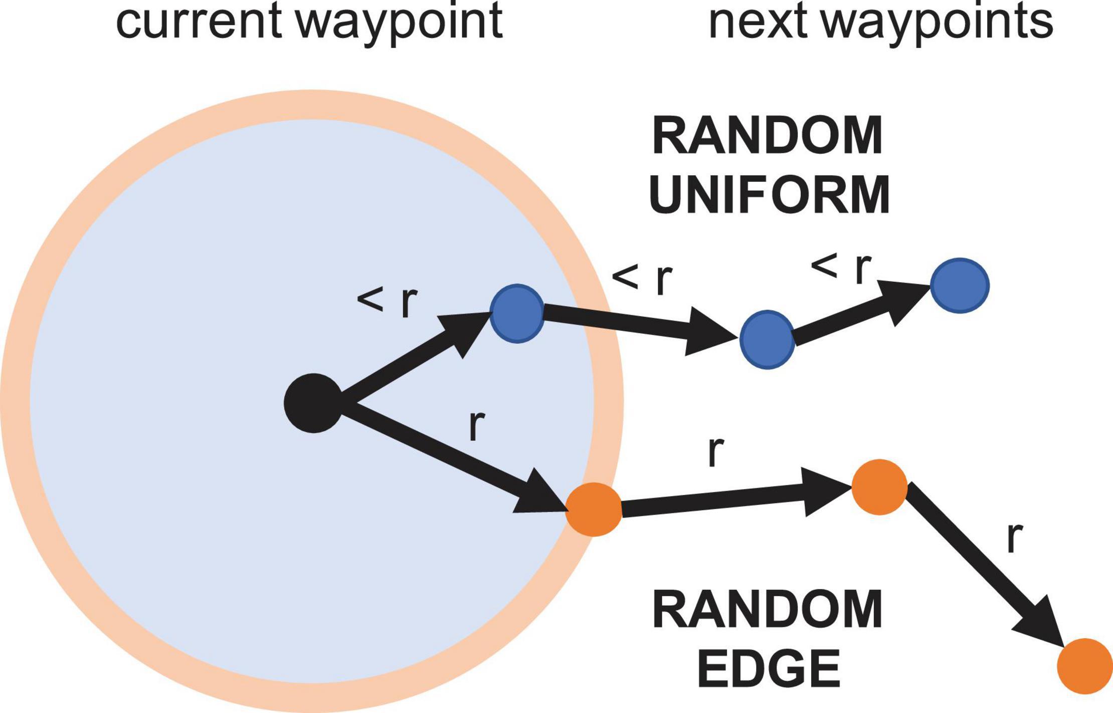
Figure 7. Visualization of the random sampling strategies. Random uniform selects any point inside a local region defined by a fixed radius r. Random edge selects any point along the region’s perimeter, potentially increasing traversed distance and coverage.

Bayesian Experimental Design

Bayesian experimental design is a framework for decision making, specifically for designing experiments that are optimal with respect to a Bayesian probabilistic criterion (Chaloner and Verdinelli, 1995). In this case, the experimental design consists of in situ samples that are to be collected in the water that will be optimally informative. Such design is derived by optimizing the expected value of a utility function that quantifies information in a probabilistic model. Here we focus on Shannon entropy H(A), which measures the average level of information or uncertainty in a random variable A (Cover and Thomas, 2006; Krause et al., 2008). It is defined as follows:

$$H(A)=-\sum _{a\in A}p(a)\log (p(a)).$$

The posterior Shannon entropy H(A|B) measures the average uncertainty of A after collecting new information B. It is given by:

$$H(A|B)=-\sum _{b\in B}p(b)\sum _{a\in A}p(a|b)\log (p(a|b)).$$

As explained earlier, our probabilistic model relies on a GP-based formulation. The posterior entropy of a GP is given by Krause et al. (2008):

$$H(A|B)=\frac{1}{2}\log \{{(2\mathrm{\pi }e)}^{dim(A)}det(\sum ^{\mathrm{\wedge }}(A|B))\}$$

In our coral reef mapping problem, the random variable of interest is the spatial distribution of spectral features throughout the remote sensing image M. Ultimately, we want to quantify the uncertainty of our coral reef mapping model given new in situ samplesP. Since our probabilistic model consists of d independent GPs, the posterior entropy of the map is additive across features; a property further explained by Cover and Thomas (2006). Then the posterior entropy of our model is given by the following expression:

$$H(M|P)=\sum _{i=1}^d\frac{1}{2}\log \{{(2\mathrm{\pi }e)}^{dim(M)}det(\sum ^{\mathrm{\wedge }i}(M|P))\}$$

Shannon entropy quantifies the uncertainty of the model M and decreases as more samples are collected (Figure 8). Consequently, an optimal sampling strategy P* would minimize entropy:

FIGURE 8

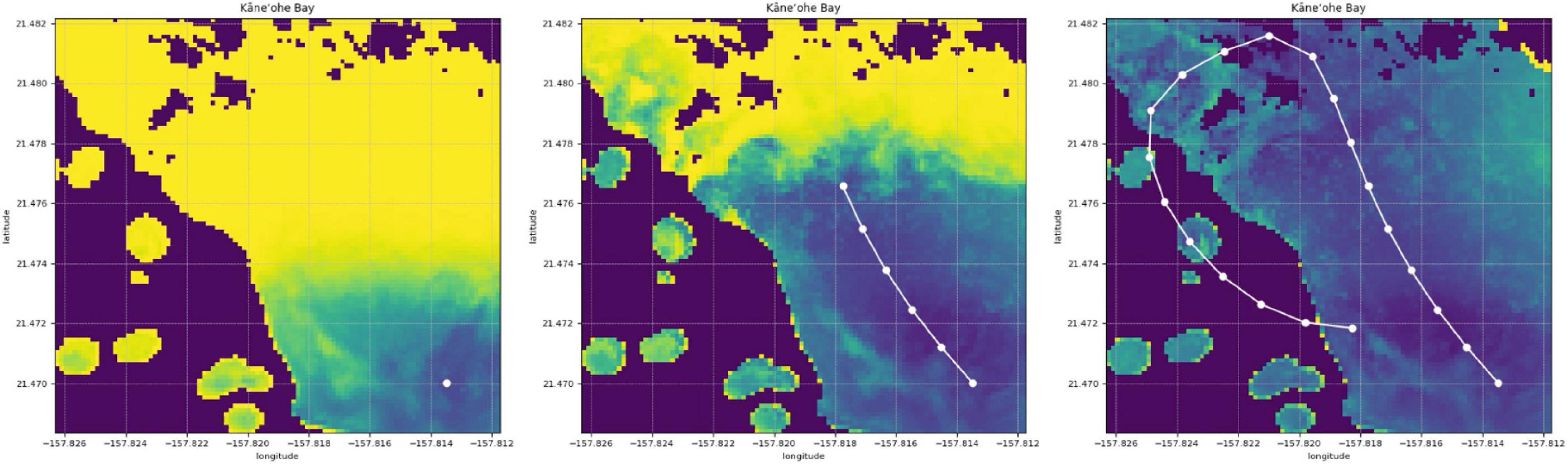
Figure 8. Visualization of the uncertainty of the model in Kaneohe Bay in terms of Shannon entropy. Light/yellow tones indicate high uncertainty areas, whereas dark blue tones denote low uncertainty. The mapping process starts with high uncertainty throughout the map (left). Uncertainty decreases as more samples are collected (center). Uncertainty is propagated throughout the scene as a function of spectral and spatial similarity in remote sensing data. Eventually there is little uncertainty left in most of the map due to the efficient extrapolation of representative samples (right).

$$P^{*}=\arg \underset{P}{\min }H(M|P)$$

Unfortunately, this optimization problem has been shown to be NP-hard (Ko et al., 1995), in other words, impossible to solve for a computer in a reasonable amount of time. The reason is that the complexity of the problem rapidly increases when evaluating each combination of possible samples. Therefore, we use and later compare two greedy heuristics that achieve near-optimal results (Krause et al., 2008). Both rely on a local-region sampling approach, similarly to our random sampling method.

Maximum entropy (ME) sampling selects one sample at a time. The next in situ sample is collected at the remote sensing pixel $\overrightarrow{v^{*}}$ with the largest individual uncertainty:

$$\overrightarrow{v^{*}}=\begin{array}{c}\hfill \arg \underset{\overrightarrow{v}}{\max }H(\overrightarrow{v})\hfill \end{array}.$$

ME sampling is relatively simple to execute, but it tends to select outliers.

An improved strategy is maximum information gain (MIG) sampling. It also selects one sample at a time. The next sample is collected at the pixel with the largest information gain, that is, with the greatest expected reduction in entropy:

$$\overrightarrow{v^{*}}=\begin{array}{c}\hfill \arg \underset{\overrightarrow{v}}{\max }H(\overrightarrow{v})\hfill \end{array}-E_{\overrightarrow{y}}[H(\overrightarrow{v}+\overrightarrow{s})]$$

MIG sampling is more expensive since it requires computation of an expectation, but it tends to outperform maximum entropy sampling by selecting more representative samples.

Monte Carlo Tree Search

Monte Carlo Tree Search (MCTS) is a heuristic search strategy that uses random trials for decision processes that are too difficult to solve. It constructs a search tree that is explored and expanded based on a random sampling process that focuses on the most promising decisions so far. MCTS integrates closely with GP models (Flaspohler et al., 2019; Candela et al., 2020). We specifically use information gain as its objective function. The main advantage against maximum information gain sampling is that MCTS is not greedy; specifically, it can look ahead multiple steps to maximize over a series of decisions. The algorithm expands branches to simulate the total information gain after multiple steps and returns the first step of the branch with the maximum total information gain. With each execution of a single step, the GPs are updated with the new sample before the next step is planned. MCTS is similar to the rapidly exploring information gathering (RIG) algorithms by Hollinger and Sukhatme (2014). They are both sampling-based approaches. However, the formulation of MCTS does rely on discretization of the environment, whereas RIG methods can operate in continuous spaces at the cost of potentially ignoring valuable samples. The algorithm we use here, developed by Kodgule et al. (2019), utilizes an 8-connected grid. It is important to note that MCTS has no conception of its total path length during execution, just a look-ahead depth. Computation time is often significantly larger when compared to other sampling planners. Nevertheless, MCTS is non-myopic and provides a high performance bound.

Ergodic Optimal Control

Ergodic theory is a mathematical framework for studying the statistical properties of dynamical systems and stochastic processes (Petersen, 1984). Ergodic optimal control leverages such concepts to derive sampling trajectories that are both smooth and informative. Regarding smoothness, our GP-based formulation is a continuous model with the inherent benefit of allowing samples anywhere, not only from discretized locations, such as a grid. Regarding informativeness, the key idea behind ergodic optimal control is to compute trajectories such that the amount of time spent in a region is proportional to the expected information gain in that region. Much research focuses on designing ergodic trajectories, often framed as coverage problems (Hussein and Stipanovic, 2007; Mathew and Mezić, 2011). We examine two algorithms specifically designed for information gathering, Spectral Multi-scale Coverage (SMC) and Projection-based Trajectory Optimization (PTO).

SMC, proposed by Mathew and Mezić (2011), provides distinct benefit of balancing exploration and exploitation (seeking new information versus confirming expectations). Additionally, it produces very smooth trajectories. Formally, the objective function is designed to maximize the rate of decay of an ergodicity metric that measures the difference between the time-averaged behavior of the trajectory and the uncertainty of the model in terms of entropy. An informative trajectory will visit high-entropy regions frequently and low-entropy regions occasionally. The model is updated after collecting a sample and a new trajectory is computed at every step to produce a path.

The PTO trajectory planning algorithm, proposed by Miller and Murphey (2013), directly optimizes ergodicity over the entire trajectory. SMC, on the other hand, improves the rate of change of ergodicity over a single step. PTO tends to generate trajectories that collect even more informative samples than SMC, but at the expense of less smoothness, more total traversed distance, and little control on step size.

Experiments

We conduct three different experiments in this work. For the first two experiments, we address automated spectral analysis. The first experiment evaluates the performance of PCA and VAE in terms of spectral feature extraction. The second experiment compares the forementioned linear and learning-based unmixing algorithms. The third experiment is the most important since it consists of a simulation study that combines and extends ideas from the previous methods and experiments. It involves active coral reef mapping and sampling in Heron Island and Kaneohe Bay using the data described in Section “Remote Sensing Data.” All experiments, training, and simulation are performed using a laptop computer with an Intel i7 processor (2.9 GHz quad-core) and 16 GB of memory.

For the first two experiments, we employ a data set that consists of 3000 spectra sampled from both PRISM flight lines. Thousand spectra are used for the training set, 1000 for the validation set, and 1000 for the test set. All these spectra are withheld from the final experiments. The 3000 spectra are sampled using the k-means++ approach (Arthur and Vassilvitskii, 2007) to ensure that their both spectra and fractional abundances are diverse and representative. To avoid overfitting, we employ early stopping during training, which is a popular approach in deep learning (Goodfellow et al., 2016). It consists in selecting the neural network weights that minimize the loss of the validation set while training (using the training set). Other approaches, such as k-fold cross-validation, are excellent to avoid overfitting, but are typically too expensive to use with neural networks.

Results and Discussion

Spectral Feature Extraction

We compare the feature extraction algorithms described in Section “Extraction of Spectral Features”: PCA and VAE. Each of these two models learns how to convert high-resolution PRISM spectra (92 bands in 420–680 nm) into a set of features, or dimensions in the latent space. Afterwards, the models are used to reconstruct spectra from features. In this experiment we observe how error changes as a function of number of features ranging from 1 to 6. Figure 9 shows the reconstruction error of the training, validation, and test sets. First, we notice that reconstruction errors are similar for the three sets, suggesting a good generalization. We observe that VAE, the non-linear model, can compress data better than linear PCA in all cases since the reconstruction error is smaller and has a smaller variance. As one would expect, average error (for both PCA and VAE) tends to decrease as more features are used since less information is lost in the compression process. Consequently, the difference between PCA and VAE is less clear for 5 or 6 dimensions. In those cases, PCA may be more appealing since it is much faster to train and apply, at least from an implementation standpoint. However, a disadvantage of PCA is that the first dimensions (features) learn most of the information while the last dimensions essentially learn just noise. In contrast, VAE tends to spread information evenly across the latent dimensions while filtering noise.

FIGURE 9

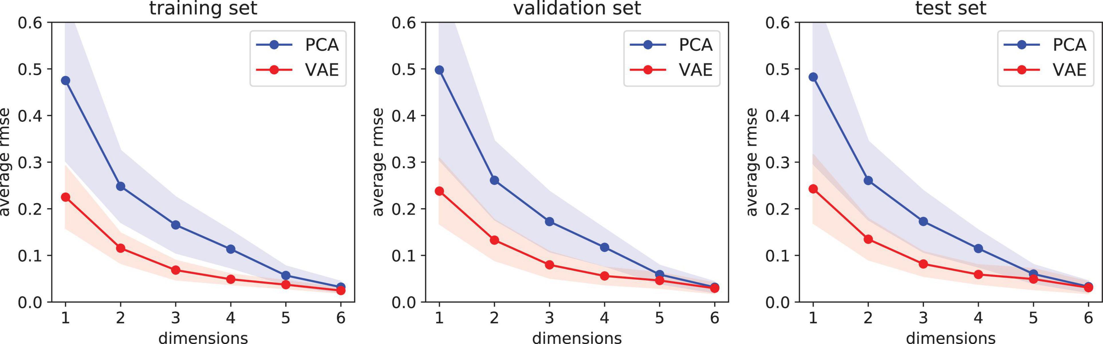
Figure 9. Reconstruction error as a function of feature dimension. Results show the average error plus-minus one standard deviation for 1000 samples in each of the three sets: training (left), validation (center), and test (right). The variational autoencoder (VAE) performs better than principal component analysis (PCA) since its reconstruction error has a smaller mean and variance. Reconstruction errors are similar for the three sets, suggesting a good generalization.

Spectral Unmixing

We compare the spectral unmixing performance of ULS, NNLS, FCLS, and NN. We use the same data set and evaluate performance in terms of two metrics that measure the difference between the predicted and real endmember abundances. These are the root mean squared error (RMSE) and the Kullback–Leibler divergence (KLD); the latter is a smooth function that measures the difference between the real and the predicted endmember abundances by treating them as probability distributions. We assume that the ground truth values are the ones estimated by Thompson et al. (2017). The associated results are shown in Table 2. We observe that linear unmixing improves as more constraints are enforced, but at the cost of losing physical meaning (e.g., negative fractional abundances are impossible in practice). Our neural network not only outperforms the linear methods, but also provides valid and consistent solutions because of its softmax output layer. The neural network is a method that is not constrained to linear representations. Another possible explanation for this result is that linear methods are very susceptible to the quality of the endmember extraction process, as well as to variability within classes.

TABLE 2

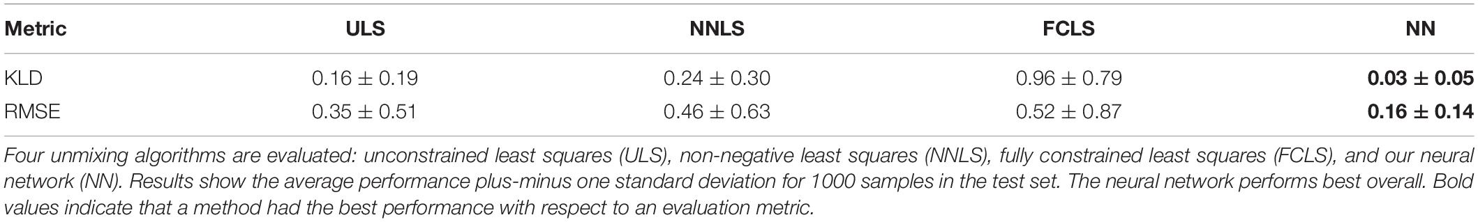
Table 2. Unmixing algorithms and their performance in terms of Kullback–Leibler divergence (KLD) and root mean squared error (RMSE).

Mapping and Sampling

This is the most important experiment in the study. It tests the ability of our approach to carry out large-scale coral reef mapping and sampling through the combination of remote sensing and in situ data. Remote sensing data comes from Landsat 8 surface reflectance products, whereas PRISM spectra are proxy for in situ samples due to high quality and resolution (both spectral and spatial).

In this experiment, we use VAE for feature extraction and the neural network for spectral unmixing because of their superior results. The data set that is used for training is withheld from this experiment. Min-max normalization is applied to both Landsat and PRISM spectra to allow the model to focus on spectral features rather than albedo values. The VAE extracts features from PRISM spectra and encodes them into a space with dimensionality d = 3. We select this value because: (1) is an intermediate value in our previous experiments, (2) VAE with d = 3 has a similar error than PCA with d = 3, and (3) false color images can be easily generated for the learned features. The overall model consists of three independent GPs that are pre-trained with the same data set, and later fine-tuned online to better adapt to incoming data.

Hundreds of sampling traverses were simulated at each of the two sites. For Heron Island, we focus on a 6 × 3 km subregion that is diverse in terms of benthic cover; for Kaneohe Bay, we focus on a smaller subregion of size 1.5 × 1.5 km (Figure 10). Forty-nine different starting locations were evenly spaced throughout each subregion; end goals were not specified. Consequently, we simulated and generated 49 traverses using each sampling algorithm, 343 traverses in total at each site. Additionally, we impose a constraint of 20 samples per traverse.

FIGURE 10

Figure 10. Experimental setting for the simulation study. A subregion of 6 × 3 km in Heron Island is shown on the left, whereas a region of 1.5 × 1.5 km in Kaneohe Bay appears on the right. Top row: abundance maps estimated by Thompson et al. (2017) and validated by the CORAL mission, serving as the ground truth in this study. Middle row: predicted abundances using the sampling strategy followed during the CORAL mission. Bottom row: predicted abundances using paths generated by two optimal sampling strategies, Maximum Information Gain (left) and Spectral Multi-scale Coverage (right). White asterisks indicate sampling locations. In this example, the optimal sampling strategies produce more accurate maps both as a function of spectral reconstruction error, in terms of Root Mean Squared Error (RMSE), and unmixing accuracy, in terms of the Kullback–Leibler Divergence (KLD).

An example of a simulated traverse at Kaneohe Bay together with its corresponding coral reef mapping process is shown in Figure 3. Signatures are successfully identified and extrapolated throughout the scene. The map is refined as more samples are collected. We observe that just a few samples (20) are sufficient to map the benthic cover of most of the 1.5 × 1.5 km area.

We analyze the performance of the seven sampling strategies discussed in subsection “Decision Theory for Sample Selection”: RU, RE, ME, MIG, MCTS, SMC, and PTO. Furthermore, we compare them with two additional approaches: a bound in which every pixel in the scene is sampled (ultimately thousands of points), and a sampling strategy that consists of the coordinates from which actual samples were collected by scuba divers during the CORAL field campaign (Figure 10). We use three metrics to evaluate the performance of the different sampling strategies in terms of mapping accuracy. For normalization purposes, we compute the averages with respect to the total number of points in the map. The first metric is the posterior entropy (Equation 3), which is directly minimized by most planners and is calculated without a ground truth. The second metric is the reconstruction error of spectra throughout the scene in terms of RMSE. It should be indirectly minimized by the planners since it always requires a basis for comparison, which is PRISM data in this case. The third metric is KLD, which measures unmixing accuracy. Furthermore, we report results with respect to three cost variables: total computation time, total traversed distance, and roughness of the traverse. The latter two are directly related to energy and time consumption. The roughness cost quantifies sudden turns along the trajectory, where perfectly straight paths receive a score of 0 degrees. Roughness is based on the smoothness scores proposed by Hidalgo-Paniagua et al. (2017) and Guillén Ruiz et al. (2020).

We use Pearson’s correlation coefficient to measure correlation between metrics throughout the simulations. Pearson’s coefficient is a measure of the strength of the linear relationship between two variables that is defined as the covariance of the variables divided by the product of their standard deviations. This is the best-known and most used type of correlation coefficient. Reconstruction error (RMSE) vs. model uncertainty (entropy) scatter plots for Heron Island and Kaneohe Bay have Pearson’s correlation coefficients of 0.881 and 0.948, respectively, 7 sampling strategies × 49 simulated traverses per sampling strategy × 20 samples per traverse. These values indicate a positive correlation between Landsat and PRISM data; they also confirm that entropy is a suitable objective function for spectral mapping. We observe a similar result when comparing KLD with entropy. The Pearson correlation coefficients are 0.937 and 0.836, demonstrating that entropy is also very useful for building accurate abundance maps. These results are also shown in Figure 11.

FIGURE 11

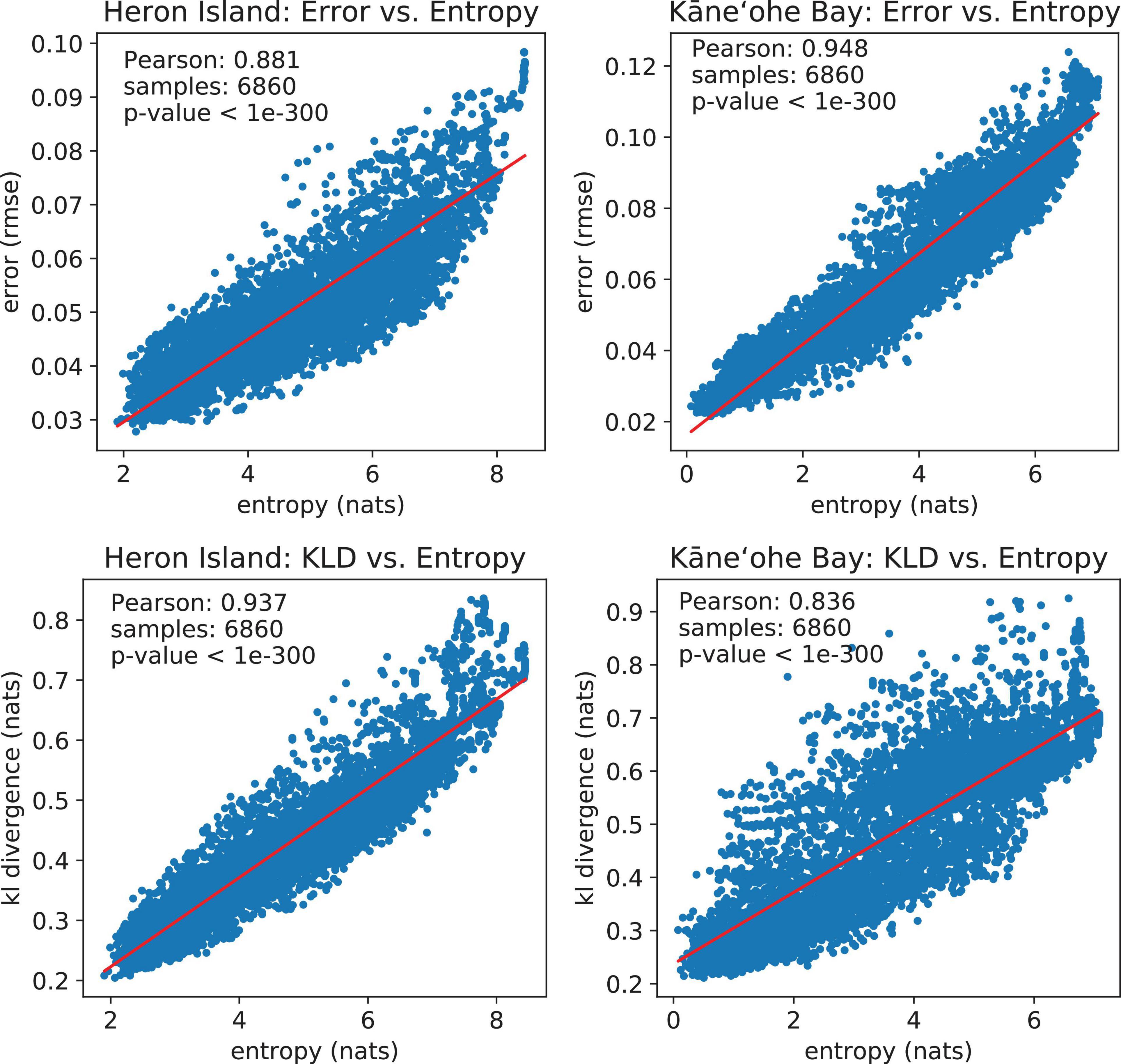
Figure 11. Top row: Spectral reconstruction error (RMSE) vs. model uncertainty (entropy). Both variables are strongly correlated according to Pearson’s correlation coefficient. Bottom row: Unmixing accuracy (KLD) vs. model uncertainty (entropy). Both variables are strongly correlated according to Pearson’s correlation coefficient.

To evaluate the performance of the various sampling strategies discussed in section “Decision Theory for Sample Selection,” the corresponding accuracy plots are shown in Figure 12, whereas the associated costs appear in Table 3. Note that Table 3 does not include cost results for the scuba diving strategy. The optimal sampling strategies generate paths, whereas the scuba diving samples were collected throughout multiple days, sometimes by more than one person; hence comparisons may not be fair. In all cases, entropy, reconstruction error, and KLD show decreasing trends that approach the optimal bound as more samples are collected. Random sampling strategies perform worst overall since they do not identify the most informative samples. Random edge is better than random uniform, apparently because it covers more distance. However, long traverses are not enough to achieve good performance since random edge is outperformed by the rest of the sampling algorithms. The greedy strategies, maximum entropy and maximum information gain, do better than random sampling. As expected, information gain is a more useful reward than bare entropy. Non-greedy approaches perform best since they look farther. PTO has the best performance scores, but at the cost of significantly longer traverses that cannot be controlled nor bounded. MCTS has similar performance scores with much more reasonable traverses, but with expensive computation times. SMC seems like an intermediate alternative with the appeal of having the smallest roughness scores overall. Interestingly, the divers’ strategy tends to score somewhere in between the random methods and the intelligent algorithms in terms of mapping accuracy (Figure 12). This seems reasonable since the divers did not formulate sample selection in terms of Shannon entropy, let alone optimized it directly; nonetheless, they were certainly executing a more intelligent strategy than mere random sampling.

FIGURE 12

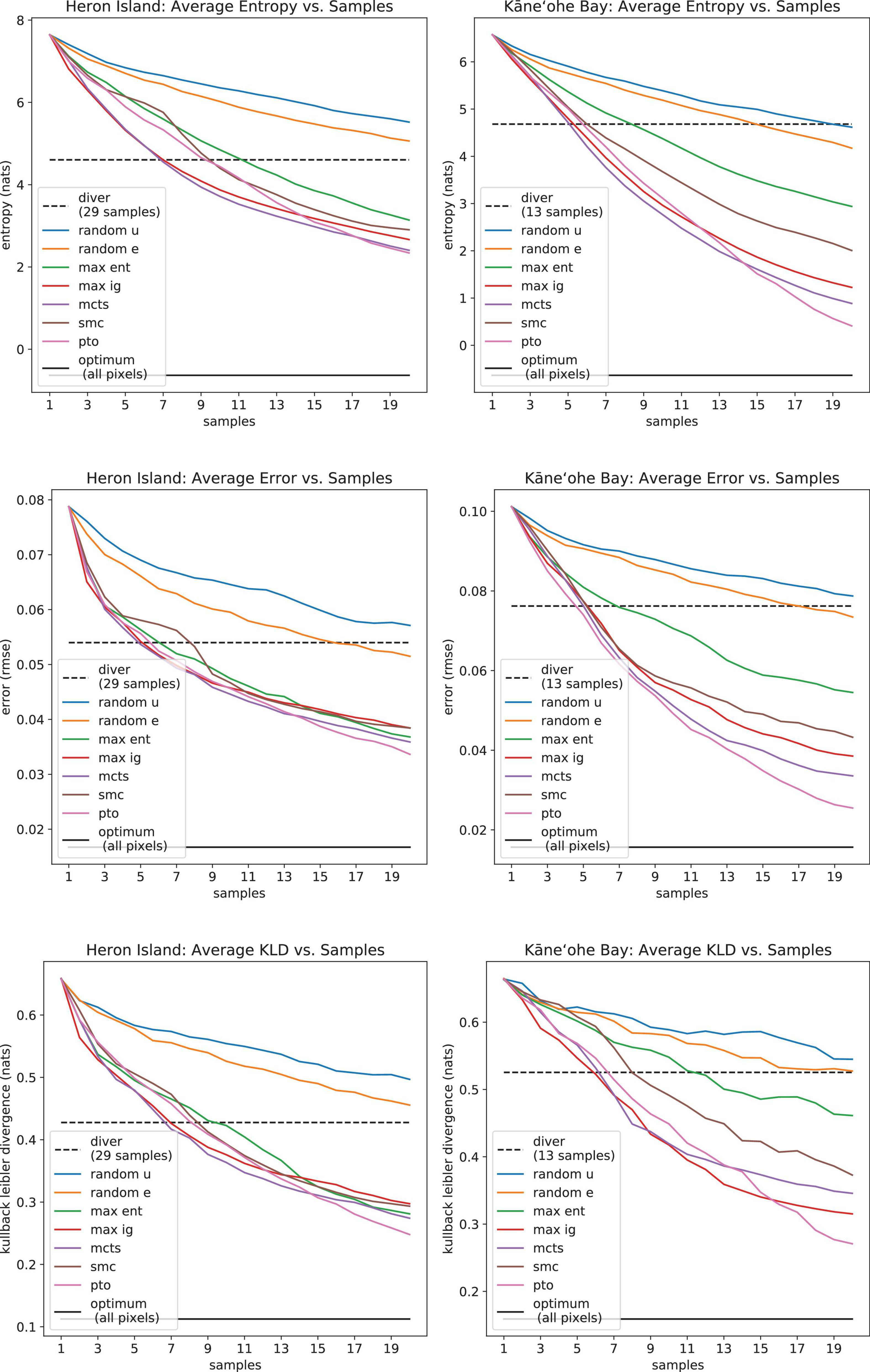
Figure 12. Average model uncertainty (Shannon entropy, top row), spectral reconstruction error (RMSE, middle row), and unmixing accuracy (KLD, bottom row) as a function of samples.

TABLE 3

Table 3. Associated costs for each sampling algorithm in terms of computation time, traversed distance, and smoothness.

Conclusion

This paper presents an approach to map coral reefs over large areas and improve the efficiency of in situ sampling. Through combination of remote sensing and in situ data, our method achieves wide-scale coverage by extrapolating relevant spectral features and by adapting to new information. This is done through a probabilistic machine learning model that fuses spectral feature extraction, spatio-spectral Gaussian process regression, and learning-based spectral unmixing. Furthermore, our approach identifies and quantifies the most valuable samples by utilizing well-defined principles of decision theory, information theory, and experimental design for sample selection. We then apply and compare various optimization techniques designed for information gathering tasks; specifically, greedy heuristics for Bayesian experimental design, Monte Carlo tree search, and ergodic optimal control.

Our simulation study using Landsat 8 and PRISM revealed key insights in the application of learning-based methods for spectral analysis and endmember mapping. We observe that hyperspectral data can be effectively compressed using linear methods like PCA, and even more accurately with non-linear methods such as VAE. Similarly, we also confirm that neural networks are powerful tools for non-linear spectral unmixing. And more importantly, we demonstrate that the combination of these methods, together with remote sensing, allows for the extrapolation of just a few in situ signatures to many locations in large areas. Ultimately the spectral reconstruction and mapping techniques presented herein lay the groundwork for application to multispectral satellite data (e.g., Landsat series, WorldView-2/3, etc.) to provide global estimates of coral reef benthic composition over time. This would represent an enormous leap in understanding the trajectory of global coral reef condition. Further, it directly improves management of coral reef ecosystems given (1) its potential to fill gaps among sparse in situ observations, especially in remote, unpopulated, or inaccessible areas, and (2) its ability to aid in design and refinement of a monitoring program – informing key locations for in situ surveys.

Regarding decision theory for informative sample selection, our results indicate that probabilistic modeling leads to substantial benefits. Concretely, we observe that Shannon entropy is strongly correlated to both spectral reconstruction error and unmixing accuracy, showing that entropy is a suitable objective function for efficient endmember mapping. We evaluate various state-of-the-art sampling strategies and conclude that they can accommodate diverse needs and constraints. PTO has the best mapping accuracy, but at the expense of very long traverses that are hard to bound. We recommend MCTS if computation time is not a critical issue. SMC appears to be a well-balanced method: it has a competitive performance with fast computation times, its traversal distances are straightforward to control, and it generates the smoothest trajectories overall, potentially resulting in significant energy and time savings.

Future investigations will improve, extend, and further validate our current model for coral reef mapping. Our results on benthic functional type mapping encourage us to pursue more complex endeavors such as coral diversity and health studies. We plan to address reef evolution over time, a thing that was not possible due to limited temporal sampling during PRISM data collection. In addition to spatial and spectral information, temporal measurements could be easily integrated into the Gaussian processes comprising our model; for instance, Gaussian processes are commonly used for time series analysis. Furthermore, we would like our model to incorporate data from other instruments. Spectrometers, despite their rich information and undeniable utility, are currently expensive to acquire and difficult to deploy in the field, especially on board AUVs. Also, spectral analysis usually requires a certain degree of expert knowledge together with access to special spectral libraries. Hence, we would like to adapt our models to instruments that may be easier to deploy for scuba divers and AUVs, such as cameras. For instance, normal images are easier for people to understand and label; besides, widely available computer vision and deep learning models could be used for automatic analysis. Finally, we intend to demonstrate the potential of our approach in the field and conduct experiments in actual coral reefs with the objective of helping divers or AUVs collect informative samples in real time.

Data Availability Statement

The original contributions presented in the study are included in the article/Supplementary Material, further inquiries can be directed to the corresponding author/s.

Author Contributions

MG, DT, GW, and DW conceived the project. AC and KE collected the data and led data analysis and modeling. AC wrote the manuscript, with contributions from all co-authors. All the authors contributed to the article and approved the submitted version.

Funding

This work was supported by funding through the Jet Propulsion Laboratory’s Strategic University Research Partnerships (SURP) Program and the National Science Foundation National Robotics Initiative Grant #IIS-1526667. AC was supported by a CONACYT Graduate Fellowship and KE was supported by a NASA Space Technology Research Fellowship.

Conflict of Interest

The authors declare that the research was conducted in the absence of any commercial or financial relationships that could be construed as a potential conflict of interest.

Publisher’s Note

All claims expressed in this article are solely those of the authors and do not necessarily represent those of their affiliated organizations, or those of the publisher, the editors and the reviewers. Any product that may be evaluated in this article, or claim that may be made by its manufacturer, is not guaranteed or endorsed by the publisher.

Acknowledgments

This research was carried out in part at the Jet Propulsion Laboratory, California Institute of Technology, under a contract with the National Aeronautics and Space Administration and funded through JPL’s Strategic University Research Partnerships (SURP) program.

Supplementary Material

The Supplementary Material for this article can be found online at: https://www.frontiersin.org/articles/10.3389/fmars.2021.689489/full#supplementary-material

References

Arthur, D., and Vassilvitskii, S. (2007). “k-means++: the advantages of careful seeding,” in Proceedings of the eighteenth annual ACM-SIAM symposium on Discrete algorithms. (Philadelphia: Society for Industrial and Applied Mathematics), 1027–1035.

Google Scholar

Binney, J., Krause, A., and Sukhatme, G. S. (2010). “Informative path planning for an autonomous underwater vehicle,” in IEEE International Conference on Robotics and Automation (ICRA), (US: IEEE), 4791–4796.

Google Scholar

Bongiorno, D. L., Bryson, M., Bridge, T. C. L., Dansereau, D. G., and Williams, S. B. (2018). Coregistered Hyperspectral and Stereo Image Seafloor Mapping from an Autonomous Underwater Vehicle. J. Field Robot. 35, 312–329. doi: 10.1002/rob.21713

CrossRef Full Text | Google Scholar

Candela, A., Kodgule, S., Edelson, K., Vijayarangan, S., Thompson, D. R., Noe Dobrea, E., et al. (2020). “Planetary Robotic Exploration Combining Remote an In Situ Measurements for Active Spectroscopic Mapping,” in In IEEE International Conference on Robotics and Automation (ICRA), (US: IEEE), 5986–5993.

Google Scholar

Candela, A., Thompson, D. R., and Wettergreen, D. (2018). “Automatic Experimental Design Using Deep Generative Models of Orbital Data,” in In International Symposium on Artificial Intelligence, Robotics and Automation in Space (i-SAIRAS), (Madrid: i-SAIRAS).

Google Scholar

Chaloner, K., and Verdinelli, I. (1995). Bayesian Experimental Design: a Review. Stat. Sci. 10, 273–304.

Google Scholar

Chollet, F. (2015). Keras. Available online at: https://keras.io (aaccessed March 31, 2021).

Google Scholar

Costanza, R., de Groot, R., Sutton, R., van der Ploeg, S., Anderson, S. J., Kubiszewski, I., et al. (2014). Changes in the global value of ecosystem services. Glob. Environ. Change 26, 152–158.

Google Scholar

Cover, T. M., and Thomas, J. A. (2006). Elements of Information Theory, 2nd Edn. Hoboken: Wiley-Interscience.

Google Scholar

Cressie, N. A. C. (1993). Statistics for Spatial Data. Hoboken: John Wiley & Sons, Inc.

Google Scholar

Eaton, M. L. (1983). Multivariate Statistics: a Vector Space Approach, 1st Edition. Hoboken: John Wiley & Sons.

Google Scholar

Flaspohler, G., Preston, V., Michel, A. P. M., Girdhar, Y., and Roy, N. (2019). Information-Guided Robotic Maximum Seek-and-Sample in Partially Observable Continuous Environments. IEEE Robot. Automation Lett. 4, 3782–3789. doi: 10.1109/LRA.2019.2929997

CrossRef Full Text | Google Scholar

Fossum, T. O., Ryan, J., Mukerji, T., Eidsvik, J., Maughan, T., Ludvigsen, M., et al. (2020). Compact models for adaptive sampling in marine robotics. Int. J. Robot. Res. 39, 127–142. doi: 10.1177/0278364919884141

CrossRef Full Text | Google Scholar

Gattuso, J.-P., Magnan, A., Billé, R., Cheung, W. W. L., Howes, E. L., Joos, F., et al. (2015). Contrasting futures for ocean and society from different anthropogenic CO2 emissions scenarios. Science 349:aac4722. doi: 10.1126/science.aac4722

PubMed Abstract | CrossRef Full Text | Google Scholar

Goodfellow, I., Bengio, Y., and Courville, A. (2016). Deep Learning. Cambridge: MIT Press.

Google Scholar

Green, E. P., Mumby, P. J., Edwards, A. J., and Clark, C. D. (1996). A review of remote sensing for the assessment and management of tropical coastal resources. Coast. Manag. 24, 1–40. doi: 10.1080/08920759609362279

CrossRef Full Text | Google Scholar

Guillén Ruiz, S., Calderita, L. V., Hidalgo-Paniagua, A., and Bandera Rubio, J. P. (2020). Measuring Smoothness as a Factor for Efficient and Socially Accepted Robot Motion. Sensors 20, 1–20. doi: 10.3390/s20236822

PubMed Abstract | CrossRef Full Text | Google Scholar

Hedley, J. D., Roelfsema, C. M., Chollett, I., Harborne, A. R., Heron, S. F., Weeks, S., et al. (2016). Remote sensing of coral reefs for monitoring and management: a review. Remote Sens. 8:118. doi: 10.3390/rs8020118

CrossRef Full Text | Google Scholar

Heinz, D. C., and Chang, C. (2001). Fully Constrained Least Squares Linear Spectral Mixture Analysis Method for Material Quantification in Hyperspectral Imagery. IEEE Trans. Geosci. Remote Sens. 39, 529–545. doi: 10.1109/36.911111

CrossRef Full Text | Google Scholar

Hidalgo-Paniagua, A., Vega-Rodríguez, M. A., Ferruz, J., and Pavon, N. (2017). Solving the multi-objective path planning problem in mobile robotics with a firefly-based approach. Soft Comput. 21, 949–964. doi: 10.1007/s00500-015-1825-z

CrossRef Full Text | Google Scholar

Hochberg, E. J., and Atkinson, M. J. (2003). Capabilities of remote sensors to classify coral, algae, and sand as pure and mixed spectra. Remote Sens. Environ. 85, 174–189. doi: 10.1016/s0034-4257(02)00202-x

CrossRef Full Text | Google Scholar

Hochberg, E. J., Atkinson, M. J., and Andrefouet, S. (2003). Spectral reflectance of coral reef bottom-types worldwide and implications for coral reef remote sensing. Remote Sens. Environ. 85, 159–173. doi: 10.1016/s0034-4257(02)00201-8

CrossRef Full Text | Google Scholar

Hochberg, E. J., and Gierach, M. M. (2021). Missing the reef for the corals: unexpected trends between coral reef condition and the environment at the ecosystem scale. Front. Mar. Sci. doi: 10.3389/fmars.2021.727038

CrossRef Full Text | Google Scholar

Hoegh-Guldberg, O., Mumby, P. J., Hooten, A. J., Steneck, R. S., Greenfield, P., Gomez, E., et al. (2007). Coral reefs under rapid climate change and ocean acidification. Science 318, 1737–1742.

Google Scholar

Hoegh-Guldberg, O., Poloczanska, E. S., Skirving, W., and Dove, S. (2017). Coral reef ecosystems under climate change and ocean acidification. Front. Mar. Sci. 4:158. doi: 10.3389/fmars.2017.00158

CrossRef Full Text | Google Scholar

Hollinger, G. A., and Sukhatme, G. S. (2014). Sampling-based Robotic Information Gathering Algorithms. Int. J. Robot. Res. 33, 1271–1287. doi: 10.1177/0278364914533443

CrossRef Full Text | Google Scholar

Hussein, I. I., and Stipanovic, D. M. (2007). Effective Coverage Control for Mobile Sensor Networks with Guaranteed Collision Avoidance. IEEE Trans. Control Syst. Technol. 15, 642–657. doi: 10.1109/tcst.2007.899155

CrossRef Full Text | Google Scholar

Kingma, D. P., and Ba, J. (2014). “Adam: a Method for Stochastic Optimization. arXiv [Preprint]. Available Online at: https://arxiv.org/abs/1412.6980 (accessed March 31, 2021).

Google Scholar

Kingma, D. P., and Welling, and Max. (2013). “Auto-Encoding Variational Bayes. arXiv. [Preprint]. Available Online at: http://arxiv.org/abs/1312.6114 (accessed March 31, 2021).

Google Scholar

Ko, C., Lee, J., and Queyranne, M. (1995). An exact algorithm for maximum entropy sampling. Operat. Res. 43, 684–691. doi: 10.1287/opre.43.4.684

PubMed Abstract | CrossRef Full Text | Google Scholar

Kodgule, S., Candela, A., and Wettergreen, D. (2019). “Non-myopic Planetary Exploration Combining in Situ and Remote Measurements,” in In IEEE/RSJ International Conference on Intelligent Robots and Systems (IROS), (US: IEEE), 536–543.

Google Scholar

Krause, A., Singh, A. P., and Guestrin, C. (2008). Near-Optimal Sensor Placements in Gaussian Processes: theory, Efficient Algorithms and Empirical Studies. J. Mach. Learn. Res. 9, 235–284. doi: 10.1145/1102351.1102385

CrossRef Full Text | Google Scholar

Kuchler, D. A., Biña, R. T., and Claasen, D. V. R. (1988). Status of high-technology remote sensing for mapping and monitoring coral reef environments. Sixth Int. Coral Reef Symp. 1, 97–101.

Google Scholar

Kumar, S., Luo, W., Kantor, G., and Sycara, K. (2019). “Active Learning with Gaussian Processes for High Throughput Phenotyping,” in In Proceedings of the 18th International Conference on Autonomous Agents and MultiAgent Systems, (Montreal: International Foundation for Autonomous Agents and Multiagent Systems), 2078–2080.

Google Scholar

Lein, J. K. (2012). Environmental Sensing: Analytical Techniques for Earth Observation, 1st Edition. New York: Springer.

Google Scholar

Maritorena, S., Morel, A., and Gentili, B. (1994). Diffuse reflectance of oceanic shallow waters: influence of water depth and bottom albedo. Limnol. Oceanogr. 39, 1689–1703. doi: 10.4319/lo.1994.39.7.1689

CrossRef Full Text | Google Scholar

Mathew, G., and Mezić, I. (2011). Metrics for ergodicity and design ergodic dynamics for multi-agent systems. Physica D 240, 432–442. doi: 10.1016/j.physd.2010.10.010

CrossRef Full Text | Google Scholar

Miller, L. M., and Murphey, T. D. (2013). “Trajectory optimization for continuous ergodic exploration,” in In: 2013 American Control Conference, (US: IEEE), 4196–4201.

Google Scholar

Moberg, F., and Folke, C. (1999). Ecological goods and services of coral reef ecosystems. Ecol. Econ. 29, 215–233. doi: 10.1016/s0921-8009(99)00009-9

CrossRef Full Text | Google Scholar

Mumby, P. J., Skirving, W., Strong, A. E., Hardy, J. T., LeDrew, E. F., Hochberg, E. J., et al. (2004). Remote sensing of coral reefs and their physical environment. Mar. Pollut. Bull. 48, 219–228.

Google Scholar

National Academies of Sciences, Engineering, and Medicine (NASEM). (2018). Thriving on Our Changing Planet: A Decadal Strategy for Earth Observation from Space. Washington: The National Academies Press.

Google Scholar

Pandolfi, J. M., Connolly, S. R., Marshall, D. J., and Cohen, A. L. (2011). Projecting coral reef futures under global warming and ocean acidification. Science 333, 418–422. doi: 10.1126/science.1204794

PubMed Abstract | CrossRef Full Text | Google Scholar

Petersen, K. (1984). Ergodic Theory. Cambridge: Cambridge University Press.

Google Scholar

Rao, D., De Deuge, M., Nourani–Vatani, N., Williams, S. B., and Pizarro, O. (2017). Multimodal learning and inference from visual and remotely sensed data. Int. J. Robot. Res. 36, 24–43. doi: 10.1177/0278364916679892

CrossRef Full Text | Google Scholar

Rasmussen, C. E., and Williams, C. K. I. (2006). Gaussian Processes for Machine Learning. Cambridge: The MIT Press.

Google Scholar

Shields, J., Pizarro, O., and Williams, S. B. (2020). “Towards Adaptive Benthic Habitat Mapping,” in IEEE International Conference on Robotics and Automation (ICRA), (US: IEEE), 9263–9270.

Google Scholar

Smith, S. V., and Buddemeier, R. W. (1992). Global change and coral reef ecosystems. Ann. Rev. Ecol. Syst. 23, 89–118.

Google Scholar

Stankiewicz, P., Tan, Y. T., and Kobilarov, M. (2021). Adaptive sampling with an autonomous underwater vehicle in static marine environments. J. Field Robot. 38, 572–597. doi: 10.1002/rob.22005

CrossRef Full Text | Google Scholar

Thompson, D. R. (2008). Intelligent Mapping for Autonomous Robotic Survey. Ph.D. thesis. Pittsburgh: Robotics Institute, Carnegie Mellon University.

Google Scholar

Thompson, D. R., Hochberg, E. J., Asner, G. P., Green, R. O., Knapp, D. E., Gao, B., et al. (2017). Airborne Mapping of Benthic Reflectance Spectra with Bayesian Linear Mixtures. Remote Sens. Environ. 200, 18–30. doi: 10.1016/j.rse.2017.07.030

CrossRef Full Text | Google Scholar

Yamada, T., Prügel-Bennett, A., and Thornton, B. (2021). Learning features from georeferenced seafloor imagery with location guided autoencoders. J. Field Robot. 38, 52–67. doi: 10.1002/rob.21961

CrossRef Full Text | Google Scholar