
95% of researchers rate our articles as excellent or good
Learn more about the work of our research integrity team to safeguard the quality of each article we publish.
Find out more
ORIGINAL RESEARCH article
Front. Mar. Sci. , 11 October 2021
Sec. Ocean Observation
Volume 8 - 2021 | https://doi.org/10.3389/fmars.2021.688815
This article is part of the Research Topic Acoustically Mapping the Ocean View all 10 articles
 Marcela Montserrat Landero Figueroa1*
 Miles J. G. Parsons2
 Benjamin J. Saunders3
 Ben Radford2
 Iain M. Parnum1
Demersal fishes constitute an essential component of the continental shelf ecosystem, and a significant element of fisheries catch around the world. However, collecting distribution and abundance data of demersal fish, necessary for their conservation and management, is usually expensive and logistically complex. The increasing availability of seafloor mapping technologies has led to the opportunity to exploit the strong relationship demersal fish exhibit with seafloor morphology to model their distribution. Multibeam echo-sounder (MBES) systems are a standard method to map seafloor morphology. The amount of acoustic energy reflected by the seafloor (backscatter) is used to estimate specific characteristics of the seafloor, including acoustic hardness and roughness. MBES data including bathymetry and depth derivatives were used to model the distribution of Abalistes stellatus, Gymnocranius grandoculis, Lagocephalus sceleratus, Lethrinus miniatus, Loxodon macrorhinus, Lutjanus sebae, and Scomberomorus queenslandicus. The possible improvement of model accuracy by adding the seafloor backscatter was tested in three different areas of the Ningaloo Marine Park off the west coast of Australia. For the majority of species, depth was a primary variable explaining their distribution in the three study sites. Backscatter was identified to be an important variable in the models, but did not necessarily lead to a significant improvement in the demersal fish distribution models’ accuracy. Possible reasons for this include: the depth and derivatives were capturing the significant changes in the habitat, or the acoustic data collected with a high-frequency MBES were not capturing accurately relevant seafloor characteristics associated with the species distribution. The improvement in the accuracy of the models for certain species using data already available is an encouraging result, which can have a direct impact in our ability to monitor these species.
Coral reef fish constitute an essential component of the continental shelf ecosystem, and a significant element of fisheries catch around the world (Anderson et al., 2009). Successful management and conservation of these demersal fishes rely on our ability to monitor their abundance and distribution. However, collecting distribution and abundance data is often expensive and logistically complex (Anderson et al., 2009). Increasing availability of seafloor mapping technologies, such as Multibeam echo-sounders (MBES), has led to the opportunity to exploit the strong relationship demersal fish species exhibit with seafloor morphology to model their distribution in a cost-effective manner (Brown et al., 2012).
Multibeam echo-sounders (MBES) are used to map the seafloor by transmitting acoustic energy toward the seafloor. The two-way travel time of this energy, to and from the transducer, combined with the angle of its travel, is used to determine the depth (bathymetry). The amount of acoustic energy reflected by the seafloor (backscatter) is used to estimate specific characteristics of the seafloor, including acoustic hardness and roughness (Fonseca and Mayer, 2007). The importance of depth to the assemblage of demersal fish has been well established (Fitzpatrick et al., 2012; Garcia-Alegre et al., 2014). As well as the direct influence depth has on demersal fish, it is also seen as a proxy for a broader set of variables involved in processes that occur at different levels of the water column which are usually harder to sample, e.g., temperature and light (Sih et al., 2017). Depth derivatives (e.g., ruggedness) are used to describe the complexity of the seafloor which can also influence the distribution of demersal fish at a variety of scales (Monk et al., 2011; Costa et al., 2014). Differences in the seafloor backscatter are used to help discriminate between benthic habitats, which can be closely related to the distribution of demersal species (e.g., sand vs. rock bottom; Monk et al., 2010; Monk et al., 2011). Therefore, the inclusion of seafloor backscatter data in demersal fish distribution models is slowly becoming more common. Multiple descriptors can be derived from the original backscatter data adding several lines of potentially useful information for species distribution modeling (Hasan et al., 2012a).
One of the most common products derived from the raw backscatter data is a mosaic, where the backscattered energy (measured as the backscatter strength on the dB scale, and backscatter intensity on the linear scale) received from different grazing angles is normalized for a certain angle or a range of angles. This method produces a regular grid usually with a resolution equal to the bathymetry layer (Fonseca et al., 2009). However, the relationship between the backscatter strength/intensity and grazing angle is related, for certain frequencies, to particular properties of the seafloor (Fonseca and Mayer, 2007). Normalizing the data to a specific angle dismisses valuable information contained in the angular response curve (ARC) (Hamilton and Parnum, 2011). Another approach is to characterize the seafloor using the Angle vs. Range Analysis (ARA) (Fonseca et al., 2009). During the ARA analysis, the backscatter response observed is compared to expected acoustic response curves based on a mathematical model, the Jackson Model (Jackson et al., 1986). In particular, the ARA analysis can be used to estimate the sediment grain size, which has been shown in some demersal species to be a driver of distribution, or at least a correlate. Previous studies have focused on testing the relevance of including the backscatter and its derivatives to model the distribution of benthic habitat classes (Ierodiaconou et al., 2007; Brown et al., 2012; Hasan et al., 2012a). Less attention has been placed in testing the benefit of adding the angular response data in modeling the distribution of demersal fishes which traditionally included the mosaic image and derivatives e.g., texture features (Hasan et al., 2014).
In the present study, terrain variables were used to model the distribution of fish data derived from Baited Remote Underwater Stereo-Video (stereo-BRUVS). The overarching aim was to test the possible improvement of a model’s accuracy if the backscatter data is included. This was tested in three areas of the Ningaloo Marine Park (NMP) with different bathymetry and levels of terrain complexity. Seven species where chosen as an indicative evaluation of the accuracy of species distribution models: starry triggerfish (Abalistes stellatus), Robinson’s seabream (Gymnocranius grandoculis), silver toadfish (Lagocephalus sceleratus), red throat emperor (Lethrinus miniatus), sliteye shark (Loxodon macrorhinus), red emperor (Lutjanus sebae), and school mackerel (Scomberomorus queenslandicus). The probability of presence of each of these species was modeled using depth, depth derivatives and backscatter (mosaic and ARC) data as explanatory variables.
Ningaloo Reef (NR) is the longest fringing coral reef in Australia, and is considered a biodiversity hotspot and to be in a good state of conservation compared with other coral reefs (Gazzani and Marinova, 2007; Schonberg and Fromont, 2012). The NMP was designed to protect 90% of these iconic waters (CALM and MPRA, 2005). A biodiversity analysis of different phyla including demersal fish, sponges, and soft corals showed the NMP is a biogeographical overlap zone, where more tropical species occur in the northern section and both tropical and temperate species are present in the southern area (Simpson and Waples, 2012). In the present study, three areas of the NMP were used to model the distribution of demersal species of fish using depth derivatives and backscatter information. Mandu in the northern area, Point Cloates in the central area and Gnaraloo in the southern zone (Figure 1).
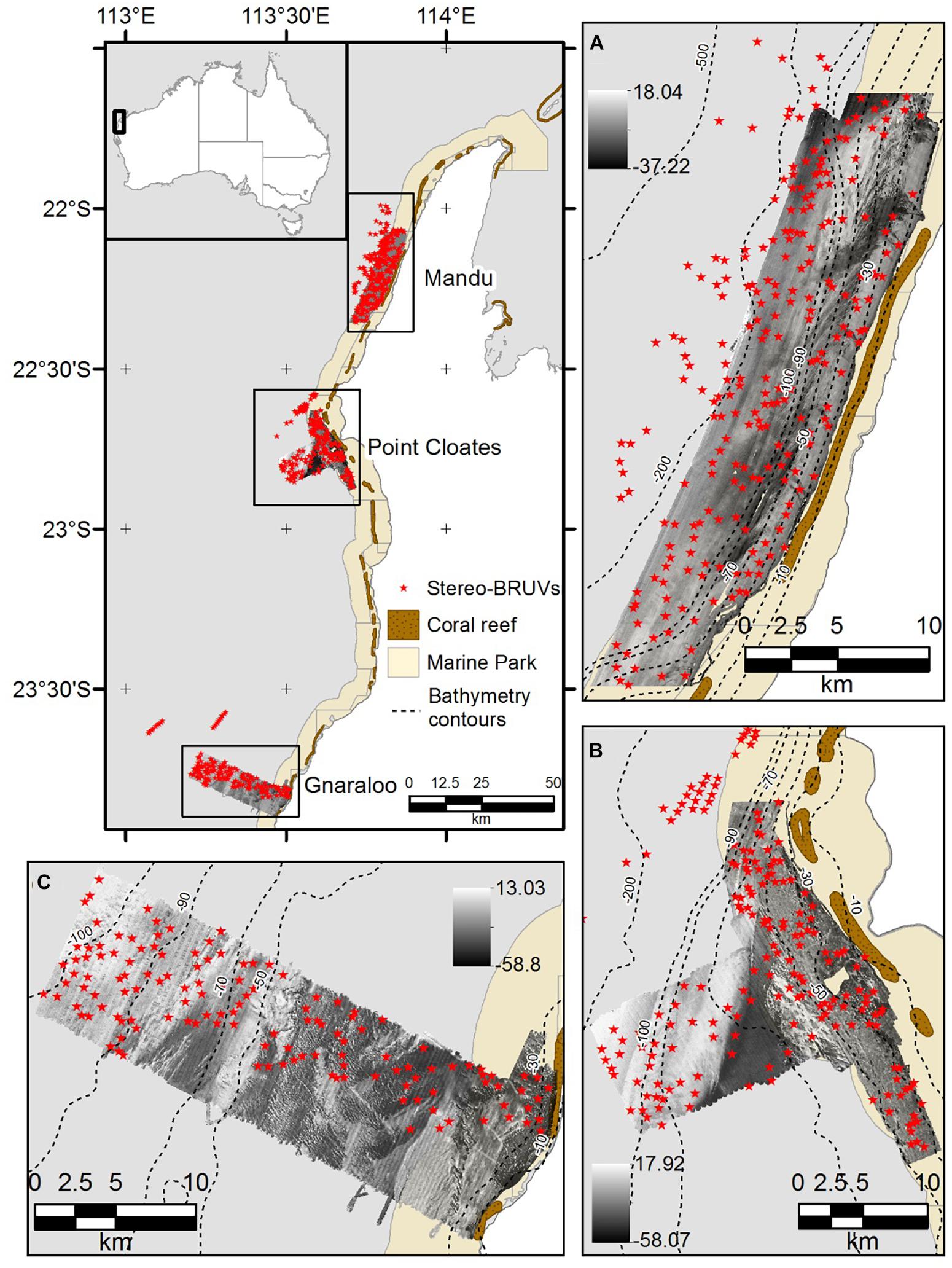
Figure 1. Study site. (A) Mandu in the northern area of the NMP, (B) Point Cloates in the central area, and (C) Gnaraloo in the southern area of the NMP. The deployment location of the stereo-BRUVS is shown as red stars, and the backscatter mosaics are shown as black and white images.
A multidisciplinary project was conducted in NMP between 2006 and 2009 by the Western Australia Marine Science Institution (WAMSI) and associates (Waples and Hollander, 2008). As part of this project, many aspects of the NMP were studied, including the demersal fish composition using Baited Remote Underwater Stereo-Video (stereo-BRUVS). A total of 656 stereo-BRUVS were deployed across the areas in Figure 1 in March-May 2009, between depths of 15 and 350 m. The stereo-BRUVS data included 239 deployments in Mandu, 185 in Pt Cloates and 155 in Gnaraloo (Waples and Hollander, 2008; Simpson and Waples, 2012). A database that included relative abundance, produced by the Australian Institute of Marine Science (AIMS), was used in the present study. The commonly used metric, MaxN, corresponds to the maximum number of individuals of the same species observed together in one frame at any one time, during the analyzed period of the video, and has been shown to provide a conservative estimate of relative abundance (Willis et al., 2000; Cappo et al., 2003). Only the first hour of recording was used for the MaxN estimation analysis, which commences the moment the cameras touch the bottom. More details on the collection and analysis of the stereo-BRUVS can be found in Harvey et al. (2007).
Depth and depth derivatives MBES surveys of the study areas were conducted in 2008 by Geoscience Australia and AIMS, using a Kongsberg EM3002, operating at 300 kHz. The MBES bathymetry was downloaded from the Geoscience Australia (GA) website as a raster with 3 m resolution. Ten depth derivatives were calculated from the bathymetry as shown in Table 1 (Moore et al., 2010, 2011). Some of the derivatives were produced using the raster package (Hijmans, 2016) of the free software R (R Development Core Team, 2017) and the rest were produced using Landserf v2.3 as specify in Table 1. Ecological processes occurring at different scales can affect the distribution and abundance of demersal fishes. Therefore, four different windows sizes were used in the production of the derivatives. The finest scale of analysis was fixed by the resolution of the MBES data (3 m) and a 3 × 3 window of analysis, while the other three were chosen based on the spatial dependence of the species. A variogram analysis was used to identify the maximum distance at which the species display spatial dependency (the range) (Holmes et al., 2008). For the species with spatial dependency, the range was above 4 km. Therefore, the scales were chosen to cover the span between the finest resolution and below the maximum range of any of the species using four windows sizes of analysis (number of cells) 3 by 3 (81 m2), 9 by 9 (729 m2), 15 by 15 (2,025 m2), and 21 by 21 (3,969 m2). The largest windows size was selected to be within the maximum range of the species, but also based on the pixel size of the ARA-phi layer (60 m). For the fractal dimension calculation, the smallest windows size allowed in Landserf is 9 by 9. Therefore, the 3 by 3 window analysis was not used for this variable.
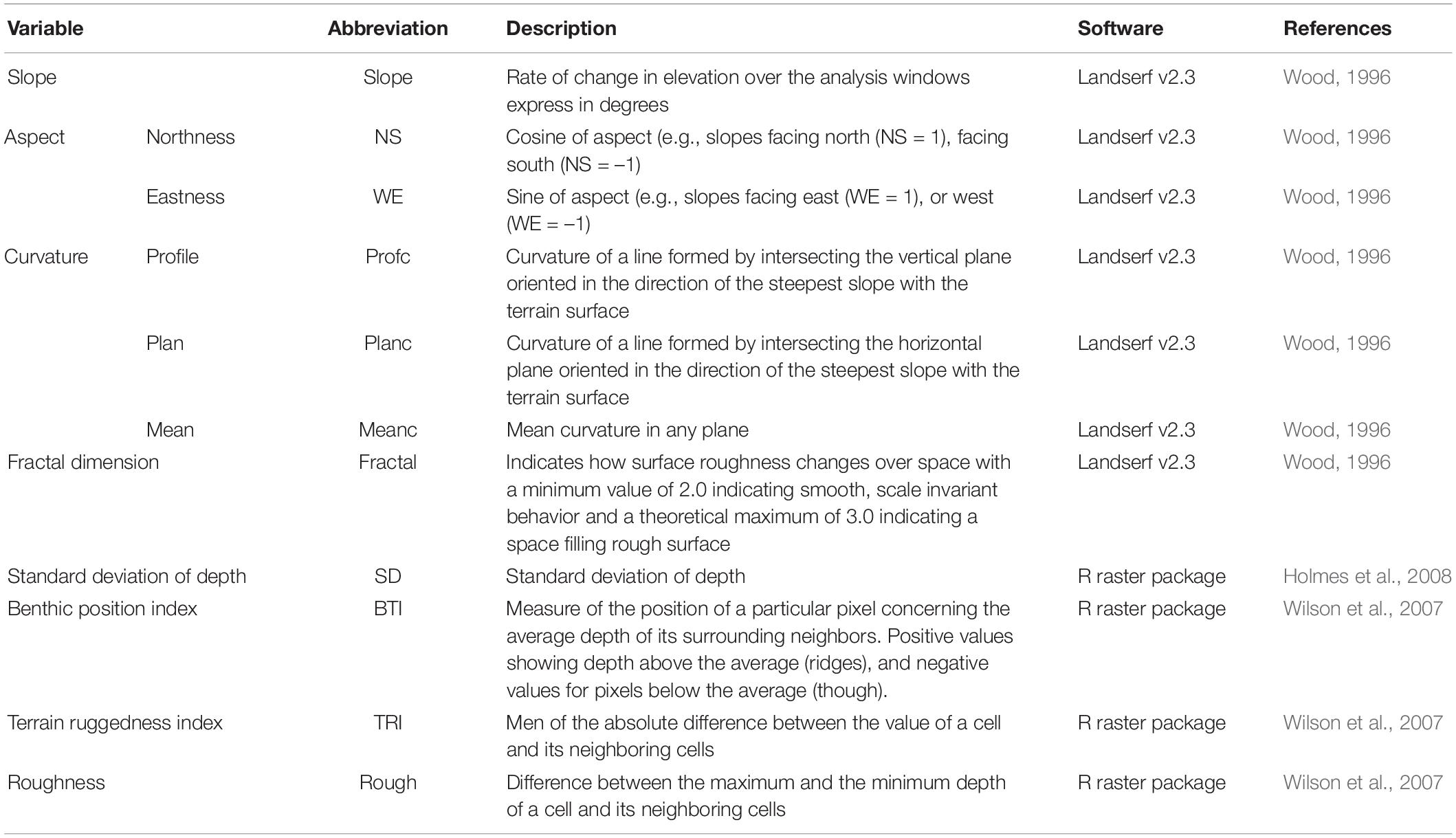
Table 1. Depth derivatives produced from bathymetry. Aspect (orientation of the slope) was divided in two variables using trigonometric transformations.
The backscatter information was included in the models as two different layers. The first one was the full-coverage, 3-m resolution mosaic, downloaded from the GA website. The second one is an approximation of the sediment phi size estimated using the ARA (Fonseca et al., 2009), applied to the raw files.
The relationship between the backscatter strength and the grazing angle is commonly known as the ARC. ARC is related, for certain frequencies, to particular properties of the seafloor (Hasan et al., 2014). Therefore, the ARC can be used to infer characteristics of the seafloor using the Angle vs. Range Analysis (ARA; Fonseca et al., 2009). In this study, we used the FMGT software (version 7.8) to conduct an ARA analysis using the raw MBES backscatter data. A full description of the method followed during the ARA analysis in FMGT can be found in Fonseca and Mayer (2007), a brief description of the method is given here.
The backscatter angular response is first corrected for radiometric and geometric distortions to locate each ping to its correct angular position. In the next step, a group of consecutive pings is stacked in the along-track direction, 30 pings were stacked. The stack of the pings produces two seafloor patches, one for the port side and another for the starboard side. The size of the patch being analyzed is approximately half of the swath of the MBES system coverage. The stacking of the pings in a patch has the effect of reducing the resolution of the final layer, but it is a necessary step to reduce the speckle noise, typical to any acoustic method. An average ARC calculated for each patch is then compared to a formal mathematical model which relates the observed backscatter with seafloor properties in a process called the ARA-inversion. During the inversion, the model is used to produce an approximation of the acoustic impedance, roughness and consequently the mean grain size of the patch under analysis. An ARA-inversion analysis was conducted for all the patches in the three studied sites to obtain maps of the distribution of grain size, with a resolution of 60 m. During the analysis, only incidence angles between 20 and 60° were included, as the angles in the near nadir and outer angle regions tend to be noisy with less power of discrimination between different types of substrate (Hasan et al., 2012b).
As part of the WAMSI project, 290 sediment samples were collected using a Van-Veen grab sampler for surface and subsurface material between 2007 and 2006 (Colquhoun et al., 2007). The grain size estimated for this ground-truth data was compared with sediment phi size estimated using the ARA analysis, correlation and regression was used to test the relationship between them.
The environmental variables including depth, depth derivatives, and the backscatter data were used as explanatory variables to explain the probability of presence of A. stellatus, G. grandoculis, L. sceleratus, L. miniatus, L. macrorhinus, L. sebae, and S. queenslandicus. The species were selected based on a minimum 25 presence in each of the sampled areas. All the species included in the present study are carnivores with different degrees of generalist feeding behavior using a variety of benthic habitats (Table 2). Lutjanids and lethirinids including G. grandoculis, L. miniatus, and L. sebae have a strong association to hard bottom or substrate with a certain degree of vertical relief (Parrish, 1987). L. sceleratus and A. stellatus, on the other hand, have a preference for sandy bottoms (Randall, 1967; Rousou et al., 2014). Seafloor backscatter can help to differentiate hard from sandy bottoms; therefore, this study has the hypothesis that the inclusion of seafloor backscatter will improve the accuracy of the models for the lutjanids and lethirinids species. For S. queenslandicus and L. macrorhinus, water column variables may be more important in explaining their distribution (Collette and Nauen, 1983; Gutteridge et al., 2011), and it is expected that the inclusion of seafloor backscatter data to have a marginal effect on their models.
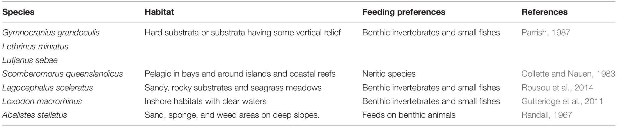
Table 2. Habitat and feeding preference of the species included in the study.
Random Forest (RF) is a robust statistical method with many advantages to solving ecological problems, including high classification accuracy and particularly high capacity to model complex interactions without statistical pre-assumptions like normality (Breiman, 2001). The algorithm begins by selecting a bootstrap sample from the data, approximately 63% of the original observations are used at least once in the bootstrap sample. The rest of the observations not selected for the bootstrap sample are called out-of-bag (OOB) observations. RF fits a tree to each bootstrap sample, but in each node, only a subsample of the variables is available for the binary partitioning (one-third of the total number of variables in the case of regression and the square root in the case of classification). All the trees are fully grown and used to predict the OOB observations. The predicted value for each observation is based on the average value predicted by the trees (Breiman, 2001). In this study, we used RF classification to model the presence/absence of the nine selected species and RF regression for the richness of species.
For the RF classification, the sensitivity and specificity were evaluated using the Area Under the Curve (AUC) of the Receiver Operator Curve. The AUC varies between 0 and 1. Values higher than 0.9 are considered outstanding whereas values between 0.9 and 0.7 indicate good performance. Values lower than 0.7 indicate poor prediction and values lower than 0.5 indicate that the model is not better than a random classification (Hosmer et al., 2013). The performance of the models was also tested using the F1, and Kappa statistics. The F1 is the harmonic mean of precision and sensitivity while the Kappa statistic (K) measures the level of chance-corrected agreement between the observed and predicted classes. According to Landis and Koch (1977) the level of agreement measured with K can be classified as K < 0.0 poor, 0 ≤ K < 0.2 slight, 0.21 ≤ K < 0.4 fair, 0.41 ≤ K < 0.6 moderate, 0.61 ≤ K < 0.8 substantial, K > 0.8 almost perfect. The effect of including the backscatter data as explanatory variables in the accuracy of the models was examined using two scenarios, the first one including depth and depth derivatives (DV) and in the second one the two backscatter variables were added (DVBS). A fivefold cross-validation procedure was used, for each fold 65 percent of the data was used to train the model and the rest to test it, an AUC, F1, and K was obtained for each fold and the mean and standard error of the statistics is reported. The difference in the mean AUC, F1, and K for the DV and DVBS scenarios was tested using a t-test in R. The mean importance of the co-variables was also calculated. For the RF regression the accuracy was measured by the mean square error (MSE), and also the percentage of variance explained by the model is reported.
A significant correlation was found in the Mandu area between the phi sediment size estimated using the backscatter data in the ARA analysis and the ground-truth sediment samples grain size (r = 0.59, p < 0.001, r2 = 0.25, p < 0.001). A significant correlation was also found in the Pt Cloates area between the phi sediment size estimated using the backscatter data in the ARA analysis and the ground-truth sediment samples grain size (r = 0.47, p = 0.003, r2 = 0.22, p < 0.001). The relationship between the grab grain size and the ARA-phi for the full data combined was also significant (p < 0.001, Figure 2). No significant correlation was found for the Gnaraloo site.
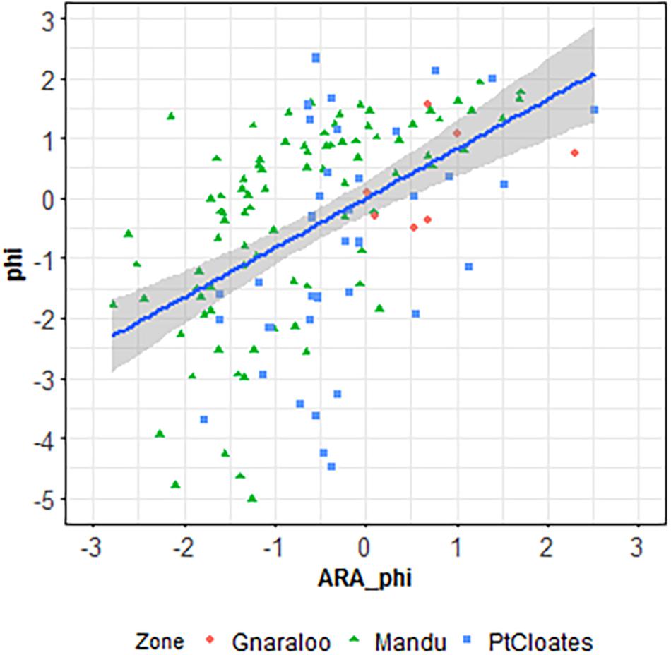
Figure 2. Linear regression between the grain size calculated with the ARA analysis and the phi size calculated from the ground-truth samples.
The performance of the models was species- and area-dependent with some species being better modeled in some areas than others and all species models having acceptable levels of accuracy (mean AUC > 0.7) in at least one of the studied sites (Figure 3A). The effect of adding the backscatter data (DVBS) also varied by species and study site with no consistent improvement in the accuracy of the models. The Mandu area had fewer models of species with acceptable levels of accuracy (mean AUC > 0.7) while Pt Cloates had only one species with model mean AUC consistently < 0.7. A similar pattern was observed in terms of K with lower values K < 0.2 in the Mandu area and higher mean K-values in the Pt Cloates area K > 0.4 considered as moderate performance (Figure 3B). The majority of the species had relatively high F1 mean > 0.7 (Figure 3C).
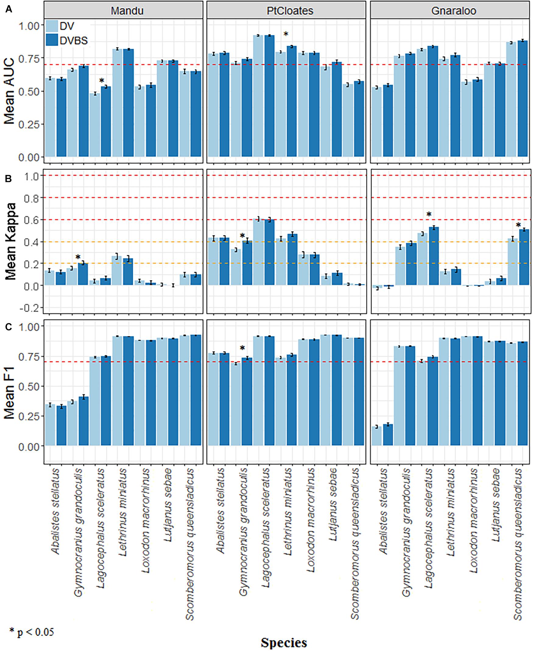
Figure 3. (A) Mean AUC, (B) Kappa, and (C) F1, and standard error of the Random Forest distribution models for A. stellatus, G. grandoculis, L. sceleratus, L. miniatus, L. macrorhinus, L. sebae, and S. queenslandicus in the three study sites of the Ningaloo Marine Park. The depth and depth derivative scenario (DV), and the depth, depth derivatives plus the backscatter data (DVBS) scenario are shown. Red dotted horizontal lines in (A,C) show AUC = 0.7 and F1 = 0.7 respectively, and for (B) the orange dotted lines indicate K = 0.2 and K = 0.4, while the red ones indicate K = 0.6 and K = 0.8. * denotes significance at the 0.05 level.
For G. grandoculis, the inclusion of the seafloor backscatter had a positive effect on the performance of the models increasing the mean AUC, K and F1 in all the three study sites. The increase on the mean value was significant for the K statistic in the Mandu and Pt Cloates area, and for the F1 in the Pt Cloates area. The significant increase of the F1 in the Pt Cloates area meant the accuracy of the resulting model was F1 > 0.7. The significant increase of the mean K also meant the model including the seafloor backscatter had an accuracy considered moderate (K > 0.4). Although the increase of the mean AUC in the G. grandoculis models was not significant, the mean AUC (± se) for Pt Cloates area was > 0.7 after the inclusion of the seafloor backscatter data (Figure 3A).
The DVBS scenario had a better performance in the models of L. miniatus, and S. queensladicus in at least two of the study sites, with different levels of improvement. The inclusion of DVBS resulted in a significant increase of the mean AUC for L. miniatus in the Pt Cloates area (Figure 3A) and a significant increase in the mean K in the S. queensladicus model in the Gnaraloo area (Figure 3B). A significant increase in the mean AUC was observed for the L. sceleratus model (Figure 3A) in the Mandu area, and a significant increase of the mean K in the Gnaraloo area (Figure 3B), when the seafloor backscatter was included; however, the mean AUC of the model in the Mandu area remained < 0.7.
The RF for the richness of demersal species explained different level of variance in the three study sites (Table 3). The model with the lowest level of mean explained variance was at Gnaraloo, although, the DVBS scenario produced a significant increase of explained variance by 5% (P < 0.05). In the Mandu area, a significant portion of variance was explained by the models, with more than 25% of mean explained variance. However, no change in explained variance was observed in the DVBS scenario. The richness of demersal fish species was particularly well modeled in the Pt Cloates area with variance explained of greater than 40%. The importance of the backscatter data was evident with an increase of the explained variance in the DVBS scenario, although the increase was not significant (Table 3).
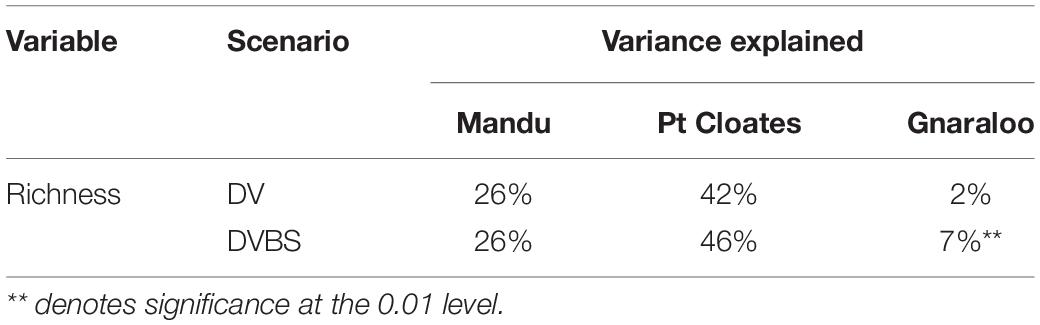
Table 3. Mean percentage of variance explained by the Random Forest for the total richness of species in the three study sites for both the depth and depth derivatives (DV, BT + DV) and depth, depth derivatives and seafloor backscatter data (DVBS, BT + DV + BS) scenarios.
A summary of the most important variables explaining the distribution of the species is shown in Table 4. Depth and seafloor backscatter were the most important variables in the construction of the models for the majority of the species in the three study sites (Table 4). Depth was key for the majority of the species in the three study areas, with some exceptions. Variables related to terrain variability (including roughness, TRI, and standard deviation of depth) were important for many of the species, in particular at a broad-scale (15–21 neighbors). For the models of L. sceleratus, L. macrorhinus, and S. queenlandicus, for example, the terrain variability variables had higher importance than depth in the Pt Cloates area.
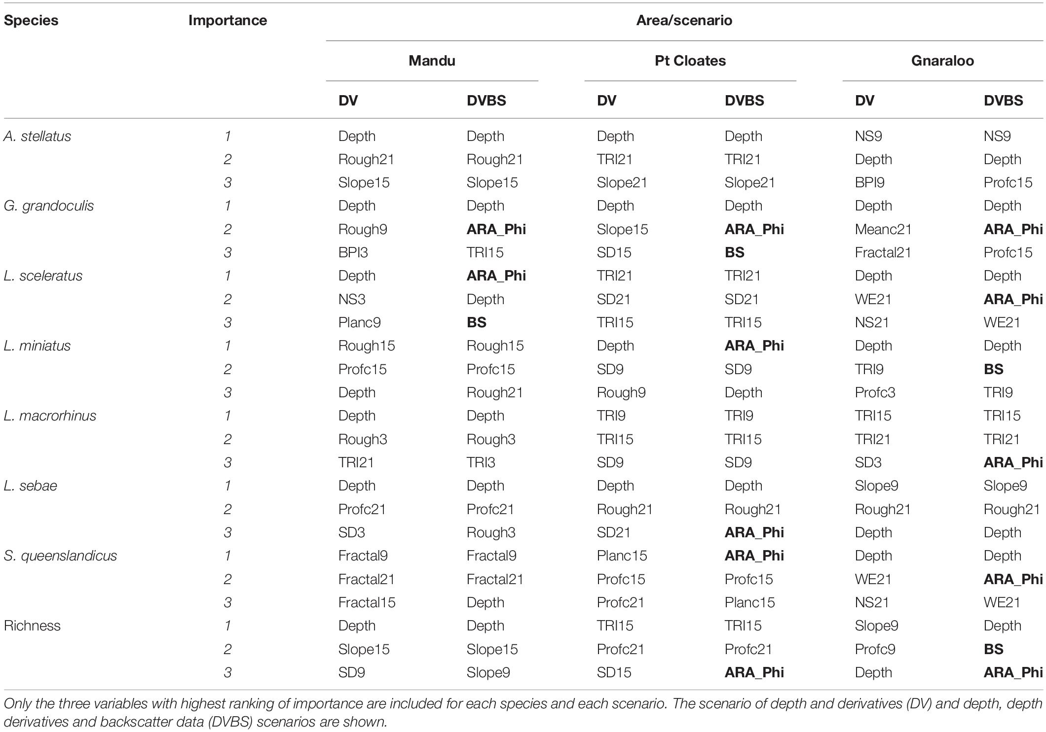
Table 4. Summary of variable importance in the construction of the distribution models for the species included in the study.
The seafloor backscatter, and the ARA-phi layer, were among the three most important variables in the models of six of the seven studied species in at least one of the study areas. For G. grandoculis, the ARA-phi was the second most important variable in the models of the three study sites, confirming its importance for this species as shown by higher mean AUC, F1 and K of the DVBS models compared to the DV scenario. For L. sceleratus DVBS models in both the Mandu and Gnaraloo areas the ARA-phi and the backscatter mosaic ranked among the three most important variables in the models. The ARA-phi variable was identified as one of the three most important variables in the models of L. miniatus, S. queenslandicus, in both Pt Cloates and Gnaraloo areas. For the L. macrorhinus and L. sebae model, the ARA-Phi was important in the Gnaraloo and Pt Cloates areas, respectively.
Depth was the most important variable in the construction of the model for the richness of species in the Mandu area, in both DV and DVBS scenarios. For the Pt Cloates area, TRI, followed by the profile curvature were the most important variables explaining the richness of species. The ARA-phi layer was also considered important when included in the model for Pt Cloates, although with a lower ranking. For the Gnaraloo area, slope, profile curvature and depth were the most important variables in the DV model, while for the DVBS model, both the ARA-phi layer and backscatter mosaic were second and third in importance.
The accuracy of the species distribution models based on depth and depth derivatives varied among species and study sites. Higher accuracies were observed, in general, for the species in the Pt Cloates area, which is considered to have a complex seafloor. The terrain variables were less successful in modeling the presence of the species in the Mandu area. The addition of the seafloor backscatter in the species distribution models did not necessarily increase the model’s accuracy in a significant manner, although, in the majority of the cases the ARA-phi layer was ranked as an important variable when included in the models. The ARA-phi layer was particularly important in the model of G. grandoculis in the three study sites, and L. miniatus in two areas, increasing the accuracy of the models. A significant portion of the species richness variation was explained using the terrain variables, and the addition of the seafloor backscatter improved the accuracy of the model in the Gnaraloo area.
A significant relationship was found between the phi size estimated with the ARA analysis and the grain sediment size measured from the grab samples. However, the ARA-phi analysis did not identify coarse gravel sediments (cobbles) with phi values below −3. Previous studies have suggested the inclusion of backscatter, and in particular, the use of the angular response of the backscatter can add to the discrimination between benthic habitats (Hasan et al., 2014). However, the seafloor backscatter intensity can be affected in different ways by the frequency of the echo-sounder, sediment grain size, nature, and magnitude of seabed roughness, and volume scattering by subsurface scatters (Ferrini and Flood, 2006). For example, previous studies have shown that the use of high-frequency MBES (e.g., 300 kHz) can lead to misclassification of coarse sediments when the grain size is larger than the acoustic wavelength of the sonar. In such cases, there is a decrease in the backscatter values for sediments of increasing grain size (i.e., λ = –2.3 ϕ, equal to 5 mm; Eleftherakis et al., 2014). In this study, something similar was observed with a significant correlation between grain size and the acoustic backscatter (ARA-phi), but low agreement between the two for large grain sizes. Also, scattering register by a high-frequency echo-sounder would be related to seabed surface roughness while scattering by particles under the sediment-water interface will be relatively more important at lower frequencies (Jackson et al., 1986). A previous study compared a high (200 kHz) and low (50 kHz) frequency echo-sounders and its ability to discriminate sediment grain size and found the higher frequency system failed to differentiate between sediment grain sizes even between mud and sand (Freitas et al., 2008). The importance of the different variables influencing the backscatter of the seafloor can also vary between sampling sites (Ferrini and Flood, 2006). Therefore the seafloor backscatter on its own has limitations to predict seabed characteristics (Ferrini and Flood, 2006).
A drawback in the approach adopted in this study was using a constant number of stack pings during the ARA analysis, as the area sampled would then depend on the water depth. As a result, the sampling areas in the shallowest depths were around three times smaller than in the deepest zones. This can produce a misinterpretation of the sediment class in deeper areas, in particular, in areas of transition between two different classes. However, the vast majority of stereo-BRUVs deployments were not located in areas of transition between different ARA-phi classes reducing the risk of mixing sediment classes. Hence, it is unlikely that the different resolutions of the ARA-phi size layer had a significant effect on the species distribution models. The high ranking of the ARA-phi in the models of species distribution, reinforce the idea that the resolution of the variable was appropriate.
For the majority of species, depth was a primary variable in explaining their distribution across the three study sites and for both DV and DVBS scenarios. Depth is a common variable influencing the distribution of species in coral reef areas, as it is related to the effects of light availability on community composition and function (Hill et al., 2014).
The importance of the depth derivatives at different window sizes varied among species and study sites. For the most abundant species, such as A. stellatus, L. sceleratus, and G. grandoculis, broader-scale variables (15 × 15 and 21 × 21 windows size) of TRI, roughness, slope and fractal dimension were considered key variables in explaining their distribution. These results agree with previous studies, showing that broad-scale variables are more relevant for species with higher mobility and larger home ranges that use a variety of benthic habitats (Franklin et al., 2009; Tamburello et al., 2015). For other species, like L. macrorhinus, which had the lowest prevalence in the study, the fine-scale variables were more important in two of the study areas, indicating a higher level of specialization. For the remaining species, a mix of fine and broad-scale variables was important in the construction of the distribution models.
The ARA-phi layer which was calculated with a broad resolution of 60 m, was found to be one of the three most important variables in the species models. This reaffirms the importance of broad-scale variables for roaming species with a wide niche (Monk et al., 2011; Moore et al., 2011). The backscatter mosaic at 3 m resolution was often included as a key variable, though to a lesser extent. This study investigated the hypothesis that the addition of the seafloor backscatter would increase the accuracy of the models, in particular, for G. grandoculis, L. miniatus, L. sebae, L. sceleratus, and A. stellatus models. Seafloor backscatter data were consistently important in the models of G. grandoculis, increasing the model’s accuracy for the three study sites. G. grandoculis is a species that inhabits rocky bottoms (Dorenbosch et al., 2005), which can explain the importance of backscatter in the construction of the models as this variable can be used to differentiate between soft/hard bottoms (Kloser et al., 2010). L. miniatus is associated with sand around coral reefs areas where it feeds on benthic invertebrates, which could explain the importance of the seafloor backscatter in the models of two of the study sites (Carpenter and Niem, 1998). However, results showed only an increase of 2–5% in the model mean AUC for G. grandoculis, L. miniatus and L. sceleratus, in at least two of the study sites, and similar incremental increases in F1 and K. Also, the increase of the mean AUC was only significant for L. sceleratus and L. miniatus, therefore the improvement can only be seen as indicative. L. miniatus is often more prevalent in shallow waters, such as on the Great Barrier Reef where it was found in 12–18 m of water (Newman and Williams, 2001), which may explain the lack of importance in the model accuracy for this species in the Mandu area. Depth might play a more important role at Mandu, where rapid changes in bathymetry are observed (Brooke et al., 2009). L. sceleratus, inhabits offshore sandy bottoms in their early life stages with a habitat shift to deeper or rocky grounds for the largest individuals (Fitzpatrick et al., 2012). The inclusion of the ARA layer may, therefore, add useful information to differentiate between sandy and rocky habitats. For L. sebae, the inclusion of the seafloor backscatter had a positive effect on the accuracy of the models for the Pt Cloates while variables measuring the rugosity of the seafloor were particularly important for this species in the three study sites. This species is associated with exposed reef slope (Fitzpatrick et al., 2012) which could explain the importance of variables related to the complexity of the seafloor as coral reef areas have, in general, higher levels of terrain complexity and rugosity.
Depth and backscatter were not considered as important in explaining the distribution of some species. For example, L. macrohinus is a small species of shark whose distribution was more related to variables measuring the rugosity of the seafloor. Another species, S. queenslandicus, is an epipelagic neritic schooling species (Collette and Nauen, 1983; Kailola et al., 1993), which might explain the poor performance of the models for this species in two of the study sites, as variables of the terrain might not be related to its distribution.
Previous studies have found the addition of backscatter metrics can be important in the construction of models of demersal fish distribution (Monk et al., 2011) or suggested further studies were needed to assess the relationship between seafloor backscatter and the assemblage of demersal fish (Schultz et al., 2014). The results of this study showed that the seafloor backscatter was an important variable in the models of demersal fish distribution. However, the inclusion of this variable did not necessarily lead to an improvement in the accuracy of the models. Possible reasons for that may be that the depth and derivatives were capturing the significant changes in the habitat, or that the substrate was not a significant driver for the species distribution.
Another factor is the uncertainty associated with the use of seafloor backscatter to approximate specific characteristics of the seafloor, including roughness and hardness, but also sediment grain size. The amount of energy reflected by the seafloor is affected by the frequency of the MBES, and although higher frequencies are more affected by seabed roughness, they have less penetration in the sediment. For example, a 100 kHz frequency in fine sediment is expected to penetrate between 0.1–1 m (Fonseca et al., 2002), while a 12 kHz can penetrate up to 12 m in muddy deposits (Schneider von Deimling et al., 2013). The level of penetration in the sediments of high frequencies is also highly sensitive to small changes in sediment properties, in particular, between fine sediments (Gaida et al., 2018). Higher frequencies are also less effective to map coarse sediment larger than the wavelength of the MBES, which will have a lower level of acoustic reflectance. Therefore, the high frequency of the MBES (300 kHz) could limit the power of discrimination between benthic habitats (Boscoianu et al., 2008; Schneider von Deimling et al., 2013), that might be relevant for habitat selection of demersal fish. The use of multi-frequencies could increase our ability to discriminate between seabed environments (Feldens et al., 2018; Gaida et al., 2020). Previous studies have shown the use of multiple frequencies, in particular lower frequencies (e.g., 100 kHz) can help differentiate between soft sediments (Costa, 2019). However, the possible improvement of benthic habitat discrimination will also be related to the characteristics of the study site, as shown by Gaida et al. (2018).
The analysis of the 656 stereo-BRUVS showed that only around 3% of the species were moderately prevalent, occurring in ≥ 20% of the sampling point (Simpson and Waples, 2012). In the present study, we included some of these species, those with a minimum of 25 occurrences on each of the three sites in an effort to compare the model performance in different areas of the NMP. Therefore, they all presented a certain degree of generalist behavior which is related to less specialized habitat requirements, and as a result it is more difficult to produce well performing models of the species distributions (Wilson et al., 2008). Finally, the combination of stereo-BRUVS with acoustic data in itself includes a certain degree of uncertainty, for example, by the use of bait which can attract fish from the areas around the deployment. The possible impact of the incorrect location of presence records in the models of species distribution will be less likely for species for which depth and ARA-phi variables were important, considering that both variables have a high local spatial autocorrelation (in an area of 500 m around the stereo-BRUVs deployment) (Naimi et al., 2014). Future studies using more than one frequency are needed to better test the benefit of using the seafloor backscatter in habitat distribution models of species of demersal fish, in particular, for non-generalist species.
Demersal species were well modeled with the depth and depth derivatives in the majority of the species analyzed, in at least one of the study sites. The addition of the backscatter data increased the accuracy of the models for some species, in particular, a consistent positive effect was observed for G. grandoculis. Depth derivatives can integrate some of the seafloor roughness information which may explain the limited benefit of adding the backscatter data in some of the species distribution models. Additional information related to the hardness/roughness not included in the depth derivatives were important for some species for which the inclusion of the backscatter data had a positive effect.
For some species the mosaic backscatter layer appeared as an important variable in explaining their distribution. In general, however, the ARA-layer was more important for the variables in the construction of the models. This is an encouraging result that demonstrates that the use of novel derivatives which take advantage of the angular response can produce models with higher accuracies. Although the increase in the accuracy of the models was not significant for the majority of the species, it can be considered an indicative result, and more efforts are needed to confirm this pattern.
The raw data supporting the conclusions of this article will be made available by the authors, without undue reservation.
The animal study was reviewed and approved by the Curtin University Ethics Committee, AEC approval number: AEC_2014_09.
ML: conceptualization, methodology, formal analysis, writing-original draft, writing-review, and editing. MP: conceptualization, supervision, writing-original draft, writing-review, and editing. BS: conceptualization, methodology, writing-review, and editing. BR: conceptualization, formal analysis, writing-review, and editing. IP: conceptualization, investigation, supervision, writing-review, and editing. All authors contributed to the article and approved the submitted version.
Consejo Nacional de Ciencia y Tecnologia (CONACYT), provided a Ph.D. scholarship CVU 230139 for ML.
The authors declare that the research was conducted in the absence of any commercial or financial relationships that could be construed as a potential conflict of interest.
All claims expressed in this article are solely those of the authors and do not necessarily represent those of their affiliated organizations, or those of the publisher, the editors and the reviewers. Any product that may be evaluated in this article, or claim that may be made by its manufacturer, is not guaranteed or endorsed by the publisher.
We would like to thank Geoscience Australia for making the bathymetry and backscatter data available and particularly Justy Siwabessy for helping provide the raw MBES data. We would also like to thank WAMSI for funding research and making data available from NMP. Stereo-BRUVS data were collected through the Western Australian Marine Science Institute (WAMSI) Node 3 Project 1 Subproject 3.1.1: Deepwater communities at Ningaloo Marine Park.
Anderson, T. J., Syms, C., Roberts, D. A., and Howard, D. F. (2009). Multi-scale fish-habitat associations and the use of habitat surrogates to predict the organisation and abundance of deep-water fish assemblages. J. Exp. Mar. Biol. Ecol. 379, 34–42. doi: 10.1016/j.jembe.2009.07.033
Boscoianu, M., Molder, C., Arhip, J., Stanciu, M. I, and Vizitiu, I. C. (2008). “Feature sets based on fuzzy reasoning for automatic sea floor characterization,” in Proceedings of the 10th WSEAS international conference on Mathematical Methods, Computational Techniques, Non-Linear Systems, Intelligent Systems, eds N. E. Mastorakis, M. Poulos, V. Mladenov, Z. Bojkovic, D. Simian, and S. Kartalopoulos (Athens: World Scientific and Engineering Academy and Society), 234–239.
Brooke, B., Nichol, S., Hughes, M., McArthur, M., Anderson, T., Przeslawski, R., et al. (2009). Carnarvon Shelf Survey Post-Survey Report. Canberra, ACT: Geoscience Australia Record.
Brown, C. J., Sameoto, J. A., and Smith, S. J. (2012). Multiple methods, maps, and management applications: purpose made seafloor maps in support of ocean management. J. Sea Res. 72, 1–13. doi: 10.1016/j.seares.2012.04.009
CALM and MPRA (eds) (2005). Management Plan for the Ningaloo Marine Park and Muiron Islands Marine Management Area 2005–2015. Perth, WA: Government of Western Australia.
Cappo, M., Harvey, E., Malcolm, H., and Speare, P. (2003). “Potential of video techniques to monitor diversity, abundance and size of fish in studies of marine protected areas,” in Potential of Video Techniques to Monitor Diversity, Abundance and Size of Fish in Studies of Marine Protected Areas, eds J. P. Beumer, A. Grant, and D. C. Smith (Queensland, QLD: University of Queensland).
Carpenter, K. E., and Niem, V. H. (1998). The Living Marine Resources of the Western Central Pacific: Bony fishes part 4 (Labridae to Latimeriidae), Estuarine Crocodiles, Sea Turtles, Sea Snakes and Marine Mammals. Rome: Food and Agriculture Organization of the United Nations.
Collette, B. B., and Nauen, C. E. (1983). Scombrids of the World: An Annotated and Illustrated Catalogue of Tunas, Mackerels, Bonitos, and Related Species Known to Date. United Nations Development Programme. Rome: Food and Agriculture Organization of the United Nations.
Colquhoun, J., Heyward, A., Rees, M., Twiggs, E., Fitzpatrick, B., McAllister, F., et al. (2007). Ningaloo Reef Marine Park Deepwater Benthic Biodiversity Survey. Metadata Report -Number 2. Crawley WA: : Australian Institute of Marine Science.
Costa, B. (2019). Multispectral acoustic backscatter: how useful is it for marine habitat mapping and management? J. Coast. Res. 35:1062. doi: 10.2112/jcoastres-d-18-00103.1
Costa, B., Taylor, J. C., Kracker, L., Battista, T., and Pittman, S. (2014). Mapping reef fish and the seascape: using acoustics and spatial modeling to guide coastal management. PLoS One 9:e85555. doi: 10.1371/journal.pone.0085555
Dorenbosch, M., Grol, M. G. G., Christianen, M. J. A., Nagelkerken, I., and van der Velde, G. (2005). Indo-Pacific seagrass beds and mangroves contribute to fish density coral and diversity on adjacent reefs. Mar. Ecol. Prog. Ser. 302, 63–76. doi: 10.3354/meps302063
Eleftherakis, D., Snellen, M., Amiri-Simkooei, A., Simons, D. G., and Siemes, K. (2014). Observations regarding coarse sediment classification based on multi-beam echo-sounder’s backscatter strength and depth residuals in Dutch rivers. J. Acoust. Soc. Am. 135, 3305–3315. doi: 10.1121/1.4875236
Feldens, P., Schulze, I., Papenmeier, S., Schoenke, M., and von Deimling, J. S. (2018). Improved interpretation of marine sedimentary environments using multi-frequency multibeam backscatter data. Geosciences 8:214. doi: 10.3390/geosciences8060214
Ferrini, V. L., and Flood, R. D. (2006). The effects of fine-scale surface roughness and grain size on 300 kHz multibeam backscatter intensity in sandy marine sedimentary environments. Mar. Geol. 228, 153–172. doi: 10.1016/j.marego.2005.11.010
Fitzpatrick, B. M., Harvey, E. S., Heyward, A. J., Twiggs, E. J., and Colquhoun, J. (2012). Habitat specialization in tropical continental shelf demersal fish assemblages. PLoS One 7:e39634. doi: 10.1371/journal.pone.0039634
Fonseca, L., Brown, C., Calder, B., Mayer, L., and Rzhanov, Y. (2009). Angular range analysis of acoustic themes from Stanton Banks Ireland: a link between visual interpretation and multibeam echosounder angular signatures. Appl. Acoust. 70, 1298–1304. doi: 10.1016/j.apacoust.2008.09.008
Fonseca, L., and Mayer, L. (2007). Remote estimation of surficial seafloor properties through the application angular range analysis to multibeam sonar data. Mar. Geophys. Res. 28, 119–126. doi: 10.1007/s11001-007-9019-4
Fonseca, L., Mayer, L., Orange, D., and Driscoll, N. (2002). The high-frequency backscattering angular response of gassy sediments: model/data comparison from the Eel River Margin, California. J. Acoust. Soc. Am. 111, 2621–2631. doi: 10.1121/1.1471911
Franklin, J., Wejnert, K. E., Hathaway, S. A., Rochester, C. J., and Fisher, R. N. (2009). Effect of species rarity on the accuracy of species distribution models for reptiles and amphibians in southern California. Divers. Distrib. 15, 167–177. doi: 10.1111/j.1472-4642.2008.00536.x
Freitas, R., Rodrigues, A. M., Morris, E., Lucas Perez-Llorens, J., and Quintino, V. (2008). Single-beam acoustic ground discrimination of shallow water habitats: 50 kHz or 200 kHz frequency, survey? Estuar. Coast. Shelf Sci. 78, 613–622. doi: 10.1016/j.ecss.2008.02.007
Gaida, T. C., Ali, T. A. T., Snellen, M., Amiri-Simkooei, A., van Dijk, T. A. G. P., and Simons, D. G. (2018). A multispectral bayesian classification method for increased acoustic discrimination of seabed sediments using multi-frequency multibeam backscatter data. Geosciences 8:455. doi: 10.3390/geosciences8120455
Gaida, T. C., Mohammadloo, T. H., Snellen, M., and Simons, D. G. (2020). Mapping the seabed and shallow subsurface with multi-frequency multibeam echosounders. Remote Sens. 12:52. doi: 10.3390/rs12010052
Garcia-Alegre, A., Sanchez, F., Gomez-Ballesteros, M., Hinz, H., Serrano, A., and Parra, S. (2014). Modelling and mapping the local distribution of representative species on the Le Danois Bank, El Cachucho Marine Protected Area (Cantabrian Sea). Deep Sea Res. Part II Top. Stud. Oceanogr. 106, 151–164. doi: 10.1016/j.dsr2.2013.12.012
Gazzani, F., and Marinova, D. (2007). “Using choice modelling to account for biodiversity conservation: non-use value for ningaloo reef,” in MODSIM07 - Land, Water and Environmental Management: Integrated Systems for Sustainability, eds L. Oxley and D. Kulasiri (Christchurch: Modelling and Simulation Society of Australia and New Zealand).
Gutteridge, A., Bennett, M., Huveneers, C., and Tibbetts, I. (2011). Assessing the overlap between the diet of a coastal shark and the surrounding prey communities in a sub−tropical embayment. J. Fish Biol. 78, 1405–1422. doi: 10.1111/j.1095-8649.2011.02945.x
Hamilton, L. J., and Parnum, I. (2011). Acoustic seabed segmentation from direct statistical clustering of entire multibeam sonar backscatter curves. Cont. Shelf Res. 31, 138–148. doi: 10.1016/j.csr.2010.12.002
Harvey, E. S., Cappo, M., Butler, J. J., Hall, N., and Kendrick, G. A. (2007). Bait attraction affects the performance of remote underwater video stations in assessment of demersal fish community structure. Mar. Ecol. Prog. Ser. 350, 245–254. doi: 10.3354/meps07192
Hasan, R. C., Ierodiaconou, D., and Laurenson, L. (2012a). Combining angular response classification and backscatter imagery segmentation for benthic biological habitat mapping. Estuar. Coast. Shelf Sci. 97, 1–9. doi: 10.1016/j.ecss.2011.10.004
Hasan, R. C., Ierodiaconou, D., and Monk, J. (2012b). Evaluation of four supervised learning methods for benthic habitat mapping using backscatter from multi-beam sonar. Remote Sens. 4, 3427–3443. doi: 10.3390/rs4113427
Hasan, R. C., Ierodiaconou, D., Laurenson, L., and Schimel, A. (2014). Integrating multibeam backscatter angular response, mosaic and bathymetry data for benthic habitat mapping. PLoS One 9:e97339. doi: 10.1371/journal.pone.0097339
Hill, N. A., Lucieer, V., Barrett, N. S., Anderson, T. J., and Williams, S. B. (2014). Filling the gaps: predicting the distribution of temperate reef biota using high resolution biological and acoustic data. Estuar. Coast. Shelf Sci. 147, 137–147. doi: 10.1016/j.ecss.2014.05.019
Holmes, K. W., Van Niel, K. P., Radford, B., Kendrick, G. A., and Grove, S. L. (2008). Modelling distribution of marine benthos from hydroacoustics and underwater video. Cont. Shelf Res. 28, 1800–1810. doi: 10.1016/j.csr.2008.04.016
Hosmer, D. W., Lemeshow, S., and Sturdivant, R. X. (2013). Applied Logistic Regression. New York, NY: Wiley.
Ierodiaconou, D., Laurenson, L., Burq, S., and Reston, M. (2007). Marine benthic habitat mapping using Multibeam data, georeferencedvideo and image classification techniques in Victoria, Australia. J. Spat. Sci. 52, 93–104. doi: 10.1080/14498596.2007.9635105
Jackson, D. R., Winebrenner, D. P., and Ishimaru, A. (1986). Application of the composite roughness model to high-frequency bottom backscattering. J. Acoust. Soc. Am. 79, 1410–1422. doi: 10.1121/1.393669
Kailola, P., Williams, M., Stewart, P., Reichelt, R., McNee, A., and Grieve, C. (1993). Australian Fisheries Resources. Canberra, ACT: Bureau of Resource Sciences.
Kloser, R. J., Penrose, J. D., and Butler, A. J. (2010). Multi-beam backscatter measurements used to infer seabed habitats. Cont. Shelf Res. 30, 1772–1782. doi: 10.1016/j.csr.2010.08.004
Landis, J. R., and Koch, G. G. (1977). The Measurement of observer agreement for categorical data. Biometrics 33:159. doi: 10.2307/2529310
Monk, J., Ierodiaconou, D., Bellgrove, A., Harvey, E., and Laurenson, L. (2011). Remotely sensed hydroacoustics and observation data for predicting fish habitat suitability. Cont. Shelf Res. 31, S17–S27. doi: 10.1016/j.csr.2010.02.012
Monk, J., Ierodiaconou, D., Versace, V. L., Bellgrove, A., Harvey, E., Rattray, A., et al. (2010). Habitat suitability for marine fishes using presence-only modelling and multibeam sonar. Mar. Ecol. Prog. Ser. 420, 157–174. doi: 10.3354/meps08858
Moore, C. H., Harvey, E. S., and Van Niel, K. (2010). The application of predicted habitat models to investigate the spatial ecology of demersal fish assemblages. Mar. Biol. 157, 2717–2729. doi: 10.1007/s00227-010-1531-4
Moore, C. H., Van Niel, K., and Harvey, E. S. (2011). The effect of landscape composition and configuration on the spatial distribution of temperate demersal fish. Ecography 34, 425–435. doi: 10.1111/j.1600-0587.2010.06436.x
Naimi, B., Hamm, N. A. S., Groen, T. A., Skidmore, A. K., and Toxopeus, A. G. (2014). Where is positional uncertainty a problem for species distribution modelling? Ecography 37, 191–203. doi: 10.1111/j.1600-0587.2013.00205.x
Newman, S. J., and Williams, D. M. (2001). Spatial and temporal variation in assemblages of Lutjanidae, Lethrinidae and associated fish species among mid-continental shelf reefs in the central Great Barrier Reef. Mar. Freshw. Res. 52, 843–851. doi: 10.1071/MF99131
Parrish, J. D. (1987). “The trophic biology of snappers and groupers,” in Tropical Snappers and Groupers: Biology and Fisheries Management, eds J. J. Polovina and S. Ralston (Boulder, CO: Westview Press), 405–463.
R Development Core Team (2017). R: A Language and Environment for Statistical Computing. Vienna: R Foundation for Statistical Computing.
Randall, J. E. (1967). Food Habits of Reef Fishes of the West Indies. Honolulu, HI: Hawaii Institute of Marine Biology University of Hawaii.
Rousou, M., Ganias, K., Kletou, D., Loucaides, A., and Tsinganis, M. (2014). Maturity of the pufferfish Lagocephalus sceleratus in the southeastern Mediterranean Sea. Sex. Early Dev. Aquat. Organ. 1, 35–44. doi: 10.3354/sedao00005
Schneider von Deimling, J., Weinrebe, W., Tóth, Z., Fossing, H., Endler, R., Rehder, G., et al. (2013). A low frequency multibeam assessment: spatial mapping of shallow gas by enhanced penetration and angular response anomaly. Mar. Pet. Geol. 44, 217–222. doi: 10.1016/j.marpetgeo.2013.02.013
Schonberg, C. H. L., and Fromont, J. (2012). Sponge gardens of Ningaloo reef (Carnarvon Shelf, Western Australia) are biodiversity hotspots. Hydrobiologia 687, 143–161. doi: 10.1007/s10750-011-0863-5
Schultz, A. L., Malcolm, H. A., Bucher, D. J., Linklater, M., and Smith, S. D. A. (2014). Depth and medium-scale spatial processes influence fish assemblage structure of unconsolidated habitats in a subtropical marine park. PLoS One 9:e96798. doi: 10.1371/journal.pone.0096798
Sih, T. L., Cappo, M., and Kingsford, M. (2017). Deep-reef fish assemblages of the Great Barrier Reef shelf-break (Australia). Sci. Rep. 7, 1–18. doi: 10.1038/s41598-017-11452-1
Simpson, C., and Waples, K. (2012). Node 3: Managing and Conserving the Marine State. Perth, WA: Western Australian Marine Science Institution.
Tamburello, N., Côté, I. M., and Dulvy, N. K. (2015). Energy and the scaling of animal space use. Am. Natural. 186, 196–211. doi: 10.1086/682070
Waples, K., and Hollander, E. (2008). Ningaloo Research Progress Report: Discovering Ningaloo–Latest Findings and Their Implications for Management in Ningaloo Research Coordinating Committee, Ningaloo Research Program. Perth, WA: Department of Environment and Conservation.
Willis, T. J., Millar, R. B., and Babcock, R. C. (2000). Detection of spatial variability in relative density of fishes: comparison of visual census, angling, and baited underwater video. Mar. Ecol. Prog. Ser. 198, 249–260. doi: 10.3354/meps198249
Wilson, M. F. J., O’Connell, B., Brown, C., Guinan, J. C., and Grehan, A. J. (2007). Multiscale terrain analysis of multibeam bathymetry data for habitat mapping on the continental slope. Mar. Geod. 30, 3–35. doi: 10.1080/01490410701295962
Wilson, S. K., Burgess, S. C., Cheal, A. J., Emslie, M., Fisher, R., Miller, I., et al. (2008). Habitat utilization by coral reef fish: implications for specialists vs. generalists in a changing environment. J. Anim. Ecol. 77, 220–228. doi: 10.1111/j.1365-2656.2007.01341.x
Keywords: demersal fish, habitat models, multibeam, seafloor backscatter, bathymetry, depth derivatives
Citation: Landero Figueroa MM, Parsons MJG, Saunders BJ, Radford B and Parnum IM (2021) Testing the Improvement of Coral Reef Associated Fish Distribution Models Based on Multibeam Bathymetry by Adding Seafloor Backscatter Data. Front. Mar. Sci. 8:688815. doi: 10.3389/fmars.2021.688815
Received: 31 March 2021; Accepted: 20 September 2021;
Published: 11 October 2021.
Edited by:
Katy Sheen, University of Exeter, United KingdomReviewed by:
Camilo Roa, Florida International University, United StatesCopyright © 2021 Landero Figueroa, Parsons, Saunders, Radford and Parnum. This is an open-access article distributed under the terms of the Creative Commons Attribution License (CC BY). The use, distribution or reproduction in other forums is permitted, provided the original author(s) and the copyright owner(s) are credited and that the original publication in this journal is cited, in accordance with accepted academic practice. No use, distribution or reproduction is permitted which does not comply with these terms.
*Correspondence: Marcela Montserrat Landero Figueroa, bW9uc2VycmF0LmxhbmRlcm9AY3VydGluLmVkdS5hdQ==; orcid.org/0000-0001-6529-0676
Disclaimer: All claims expressed in this article are solely those of the authors and do not necessarily represent those of their affiliated organizations, or those of the publisher, the editors and the reviewers. Any product that may be evaluated in this article or claim that may be made by its manufacturer is not guaranteed or endorsed by the publisher.
Research integrity at Frontiers
Learn more about the work of our research integrity team to safeguard the quality of each article we publish.