 Leonardo Azevedo
 Luís Matias2
95% of researchers rate our articles as excellent or good
Learn more about the work of our research integrity team to safeguard the quality of each article we publish.
Find out more
ORIGINAL RESEARCH article
Front. Mar. Sci. , 12 August 2021
Sec. Ocean Observation
Volume 8 - 2021 | https://doi.org/10.3389/fmars.2021.685007
This article is part of the Research Topic Acoustically Mapping the Ocean View all 10 articles
A two-dimensional multichannel seismic reflection profile acquired in the Madeira Abyssal Plain during June 2016 was used in a modeling workflow comprising seismic oceanography processing, geostatistical inversion and Bayesian classification to predict the probability of occurrence of distinct water masses. The seismic section was processed to image in detail the fine scale structure of the water column using seismic oceanography. The processing sequence was developed to preserve, as much as possible, the relative seismic amplitudes of the data and enhance the shallow structure of the water column by effectively suppressing the direct arrival. The migrated seismic oceanography section shows an eddy at the expected Mediterranean Outflow Water depths, steeply dipping reflectors, which indicate the possible presence of frontal activity or secondary dipping eddy structures, and strong horizontal reflections between intermediate water masses suggestive of double diffuse processes. We then developed and applied an iterative geostatistical seismic oceanography inversion methodology to predict the spatial distribution of temperature and salinity. Due to the lack of contemporaneous direct measurements of temperature and salinity we used a global ocean model as spatial constraint during the inversion and nearby contemporaneous ARGO data to infer the expected statistical properties of both model parameters. After the inversion, Bayesian classification was applied to all temperature and salinity models inverted during the last iteration to predict the spatial distribution of three distinct water masses. A preliminary interpretation of these probabilistic models agrees with the expected ocean dynamics of the region.
Fine-scale ocean processes happening on ranges from a few meters to a few kilometers have a profound impact on turbulent dynamics, on the ocean energy budget, on primary production and ecosystems, on gas and tracer exchange, and ultimately on the global ocean circulation and climate (e.g., Wunsch and Ferrari, 2004; Mahadevan, 2016). Yet, ocean measurements at high resolutions are limited to fixed point probes or profiling devices. Therefore, quasi-synoptic measurements of simultaneously vertical and lateral high resolutions require detailed planning and the combination of several probing devices, which are not globally available to sample the ocean (Pascual et al., 2017).
Seismic oceanography (SO) is an interdisciplinary research field that uses common marine multichannel seismic reflection (MCS) data to capture high-resolution images of the ocean’s thermohaline structure. This geophysical technique has proven its value in imaging the oceanic structures with an unprecedent detail both in the horizontal and vertical directions in different basins worldwide (Holbrook et al., 2003; Hobbs et al., 2007; Ruddick et al., 2009; Pinheiro et al., 2010). SO data are indirect information of relevant oceanographic features and complement the information provided by conventional oceanographic casts, which are direct measurements of the ocean properties but sparsely distributed. More recently, these data have been used to estimate the oceanic turbulent dissipation (Holbrook et al., 2013; Sallarès et al., 2016; Dickinson et al., 2017; Fortin et al., 2017) and to estimate the spatial distribution of the ocean’s temperature and salinity using amplitude-vs.-offset analysis (Páramo and Holbrook, 2005), deterministic seismic oceanography inversion methods (Wood et al., 2008; Sallarès et al., 2009; Papenberg et al., 2010; Kormann et al., 2011; Song et al., 2012; Bornstein et al., 2013; Biescas et al., 2014; Padhi et al., 2015; Blacic et al., 2016; Dagnino et al., 2016, 2018; Minakov et al., 2017; Gunn et al., 2018; Tang et al., 2018, 2019; Gunn et al., 2020), stochastic seismic oceanography inversion (Tang et al., 2016; Azevedo et al., 2018; Jun et al., 2019) and automatic velocity analysis (Chhun and Tsuji, 2020).
In SO, multichannel seismic reflection data is processed to boost the amplitudes corresponding to seismic reflections occurring at interfaces between water layers of different temperature and salinity, where water temperature is the most important property and contributes on average 80% to the reflection coefficient (Ruddick et al., 2009; Sallarès et al., 2009). A challenge for SO data processing is the ability to image reflections near the sea surface, as traditional seismic processing sequences fail to successfully mitigate the effect of the direct wave traveling from source to receivers on the very weak reflections in the near-surface water layer (e.g., Ruddick et al., 2009; Pinheiro et al., 2010). Several processing workflows have been proposed to tackle this limitation. Huang et al. (2012) used an adaptive subtraction scheme. Hardy et al. (2007) and Jones et al. (2008) combined linear moveout with dip filtering. Ristow et al. (2017) used a combination of a linear Radon transformation with adaptive subtraction. Often, another source of coherent noise originates from the echo of the previous shot, but this noise is not addressed herein. The objective of the seismic oceanography processing shown herein is twofold: (1) to effectively attenuate the direct arrival effect using a combination of linear moveout, horizontal median filtering and adaptive subtraction; and (2) to preserve the relative seismic amplitudes of the seismic data. The attenuation of the direct wave arrival ensures a good image of the water structure in the first few hundred of meters, whereas preservation of original amplitudes is required to invert the seismic data for the ocean’s physical properties.
Seismic oceanography data represent an indirect measurement of the physical properties of the water column such as temperature and salinity. In fact, seismic reflections present in SO data originate from the interfaces between water masses with distinct properties. From an oceanographic perspective, having the ability to predict the spatial distribution of such properties from SO data would provide insights about oceanographic processes not detected by conventional oceanographic sampling techniques. The spatial prediction of such properties from seismic oceanography data is an inverse problem. Mathematically, seismic oceanography inversion can be expressed as:
where F is the forward operator through which the recorded seismic amplitudes (dobs), with dobsϵRd, are obtained from an ocean’s model, mϵRm, and e represents the error term associated with the observations and modeling uncertainties errors present in the seismic oceanography data. In the seismic oceanography case, the ocean’s acoustic properties (P-wave propagation velocity and density), m, can be computed from temperature and salinity using the thermodynamic equation of seawater (IOC, SCOR, and IAPSO, 2010).
Seismic inversion methods can be broadly divided in two different classes: deterministic or statistical (Bosch et al., 2010). Deterministic approaches are based on regression models of optimization algorithms providing a single best-fit solution. In deterministic seismic inversion the uncertainty assessment is limited and defined as a linearization around the best-fit inverse solution, which is normally retrieved by least squares, and in this sense, the uncertainty is strictly represented by a local multivariate Gaussian (Tarantola, 2005). In statistical seismic inversion, the solution is expressed as a probability density function in the model parameters space. Therefore, these inversion methods provide a set of alternative models as solution and allow the assessment of the uncertainty associated with the inverted models (Tarantola, 2005). Assessing the uncertainty about the predictions in seismic inversion is critical in any modeling procedure. The uncertainty represents the lack of knowledge about the system under investigation, measurement errors and physical approximation during the data processing (Tarantola, 2005). Also, accounting for uncertainty, and therefore risk, leads to better-informed decisions.
There are different statistical-based seismic inversion methods. These seismic inversion methodologies are iterative procedures based on different stochastic optimization algorithms such as simulated annealing, genetic algorithms, probability perturbation method, gradual deformation, geostatistical simulation and neighborhood algorithm (e.g., Sen and Stoffa, 1991; Bortoli et al., 1993; Sambridge, 1999; Le Ravalec-Dupin and Noetinger, 2002; Soares et al., 2007; González et al., 2008; Grana et al., 2012; Azevedo et al., 2015; Azevedo and Soares, 2017).
Iterative geostatistical seismic inversion methods allow predicting models at higher resolution than the observed data due to their ability to incorporate high-resolution information provided by existing direct observations (e.g., Azevedo and Soares, 2017). This is particularly of interest in oceanographic studies as it might open a window to a reality not yet known. Conventional ocean models built exclusively from the interpolation of sparse direct measurements of ocean properties, such as CTD and/or XBT, are always a smooth representation of the true ocean variability and are unable to describe complex features in detail due to the large distances between observations. The inverted models of the ocean properties retrieved from SO data are much richer from a spatial perspective as the SO data constrains the model predictions far from the location of the direct observations (e.g., Dagnino et al., 2016).
In a preliminary work, geostatistical inversion has been successfully applied to predict the spatial distribution of ocean temperature and salinity from seismic oceanography data (Azevedo et al., 2018). These authors showed how geostatistical SO inversion could retrieve a set of high-resolution temperature and salinity models that generate synthetic SO data consistent with observations. Each model represents an alternative scenario that fits equally well the observed data SO data. However, in this approach the model perturbation technique (i.e., geostatistical simulation) (Deutsch and Journel, 1992) requires the existence of contemporaneous and collocated direct measurements of temperature and salinity (e.g., CTD/XBT casts) along the SO section to be inverted. The simultaneous acquisition of CTD/XBT data is difficult due to both operational challenges and costs, and represents a major drawback in the practical use of this technique.
The main objective of this work is to propose an alternative geostatistical SO inversion method to overcome the need for contemporaneous and collocated direct observations of temperature and salinity, which might open the door to the generalization of this type of inversion method in SO studies. Low-resolution models of temperature and salinity are extracted from large-scale ocean simulations and integrated as part of the objective function within the geostatistical SO inversion method. The low-resolution models represent a background model with the expected spatial trend of temperature and salinity (Pereira et al., 2019). In practice the background models act as spatial constraints in the inversion procedure. These models are not included as part of the model parameter space to avoid limiting the exploration of the model parameter space and therefore in a limited uncertainty assessment. The marginal and joint distributions of temperature and salinity, necessary to perform the geostatistical simulations, are borrowed from quasi-contemporaneous and quasi-collocated ARGO floats profiles (Argo, 2000) which were acquired approximately simultaneous during the acquisition of the MCS profile.
As part of the proposed workflow, and to interpret the inverted models obtained in the last iteration of the inversion procedure, we classified the set of inverted models generated during the last iteration of the geostatistical SO inversion into distinct water masses using Bayesian classification (Avseth et al., 2005). From the classified models we computed the probability of occurrence of each water mass. The most likely depths of the different water masses agree with the expected values for the area of interest as proposed by other authors (Comas-Rodríguez et al., 2011).
The following section presents a detailed description of the proposed geostatistical SO inversion methodology and the Bayesian classifier used to predict the spatial distribution of the expected water masses. The proposed inversion method is then applied to a MCS profile acquired over the Madeira abyssal plain (MAP) that was specifically reprocessed for this purpose. The tailored seismic processing workflow is described in the subsequent section. We then show a preliminary and global interpretation of the oceanographic insights provided by the inverted models. The workflow proposed in this work can be applied to other locations worldwide where no contemporaneous direct measurements of salinity and temperatures and global ocean models exist in the vicinity of the seismic profiles.
The proposed iterative geostatistical SO inversion method inverts SO data directly for temperature and salinity when no contemporaneous direct observations of the ocean are available. It can be considered an extension of the method introduced by Azevedo et al. (2018). It allows the simultaneous integration of high-resolution direct measurements of temperature and salinity, such as CTD and XBT data, and background models from climatology, data products or numerical ocean simulations. A relevant aspect of the proposed method is that the background models do not constrain the model generation (e.g., used for example as a local mean during the geostatistical simulation), but are included as part of a two-term objective function where they act as a spatial regularizer (Pereira et al., 2019).
The proposed iterative geostatistical SO inversion method can be divided into four main steps: (i) generation of temperature and salinity background models; (ii) generation of high-resolution temperature and salinity models using stochastic sequential simulation and co-simulations; (iii) multi-objective mismatch evaluation; (iv) stochastic update and generation of a new set of models.
In the application example shown herein, two-dimensional large-scale temperature and salinity sections, describing the expected background spatial distribution, were retrieved from global numerical simulations of ocean dynamics provided by the Copernicus Marine Environment Monitoring Service (CMEMS, 2016). These sections were extracted for the same geographical location, acquisition date and time of the available SO section. From a geophysical inversion point of view, these simulated profiles can be thought as low-frequency models in conventional seismic inversion methodologies (e.g., Sams and Carter, 2017; Pereira et al., 2019).
Contemporaneous observed high-resolution temperature and salinity vertical profiles acquired close to the seismic oceanography profile were used to infer the marginal and joint distributions of both ocean properties. This information was used during the model generation and perturbation and not as spatial constraining data. These data were used as target marginal and joint distributions to be reproduced by the geostatistical simulation algorithms. In this inversion method, water temperature models are generated with direct sequential simulation (DSS; Soares, 2001) and salinity models were co-simulated with co-DSS with joint probability distributions (Horta and Soares, 2010). The sequential generation of models ensures that the observed relationship between temperature and salinity is reproduced in any given pair of models generated during the iterative procedure. This is essential to guarantee the plausibility of the predicted location and extent of water masses and for classification of distinct water masses as shown below.
The pairs of temperature and salinity models are used to compute water density and P-wave propagation velocity using the international thermodynamic equation of seawater (IOC, SCOR, and IAPSO, 2010). Then, normal incidence reflection coefficients are computed and convolved with a representative wavelet. In cases where contemporaneous and collocated vertical profiles of salinity and temperature are available, the wavelet can be estimated by comparing synthetic seismic traces with the real data (i.e., as in conventional seismic-to-well tie). For this work, however, the wavelet was extracted from the processed SO data by averaging the primary seafloor reflection of several traces selected from a region of relatively flat bathymetry, following the approach used by Warner (1990). The resulting synthetic traces are then compared against the corresponding real traces following:
where xs and ys are the real and synthetic seismic traces, respectively, with N seismic samples. The similarity, S, like the Pearson’s correlation coefficient is bounded between −1 and 1, but ensures a simultaneous match of the synthetic seismic on both waveform and amplitude values of the recorded SO data. The plausibility of the inverted models depends on the reproduction of both properties of the observed data.
The deviations (dev) of each single realization of temperature and salinity from the background ocean models are computed following:
where msim is a realization of temperature or salinity and mbackground is the corresponding background model. Finally, a two-term objective function (OF) is computed combining Eqs. (2) and (3):
where w1 and w2 are user defined weights that sum to 1 and control the influence of each term depending on the quality of the existing SO data and the reliability of the background model; devT and devS are the deviations of the simulated parameter from the background model for temperature and salinity, respectively. If the quality of the SO data is low, then w1 should decrease. Similarly, if the reliability of the background temperature and salinity is poor, w2 should be reduced. In the application example shown herein w1 and w2 were set by trial-and-error. However, these can be optimized under an optimization framework (e.g., Gennert and Yuille, 1988; Mead, 2008; Marler and Arora, 2010). Notice that OF is also bounded between −1 and 1 so it can be used as a proxy of a collocated correlation coefficient in the geostatistical co-simulation of a new set of temperature and salinity models in the subsequent iteration of the inversion (e.g., Soares, 2001).
For a given iteration (j), the pairs of temperature and salinity traces (i.e., vertical columns of grid samples) that ensure the maximum OF values are stored in auxiliary temperature and salinity models along with the corresponding OF values. These models are used as secondary variables in the co-simulation of a new set of models in the subsequent iteration. In practice, regions of the seismic profile with low OF will exhibit a large variability of simulated values within the ensemble of simulated models, while region of high OF will produce similar models in the next iteration.
The proposed iterative geostatistical SO inversion method is summarized in the following sequence of steps (Figure 1):
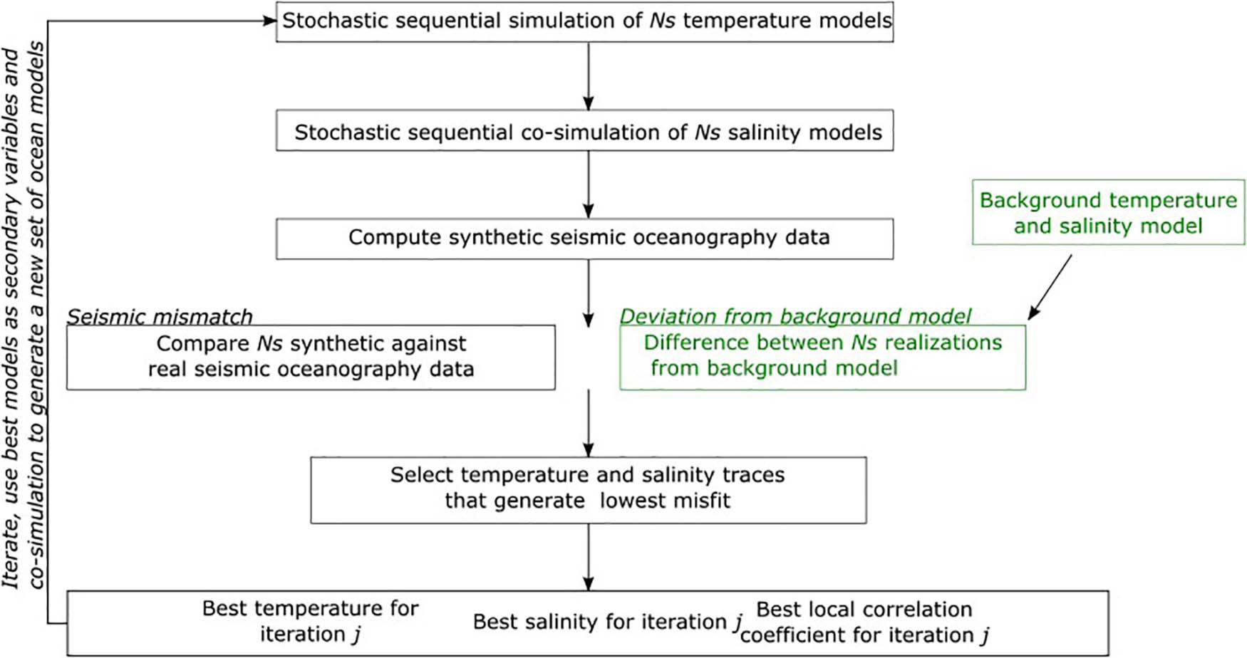
Figure 1. Schematic representation of the proposed geostatistical SO inversion including temperature and salinity background models. Green boxes represent the steps related to the integration of background ocean models.
(i) Create temperature and salinity background models for the entire inversion grid. The background models might be vertical sections extracted from numerical ocean simulations collocated with the existing SO data for the same acquisition time;
(ii) Stochastic sequential simulation (direct sequential simulation; Soares, 2001) of Ns temperature models for the entire inversion grid. Direct temperature measurements located nearby the location of the SO profile are used to infer the conditioning distribution;
(iii) Stochastic sequential co-simulation (direct sequential co-simulation with joint probability distributions; Horta and Soares, 2010) of Ns salinity models for the entire inversion grid. Direct salinity measurements located nearby the region of interest are used to infer the conditioning distribution. Each temperature model simulated in ii is used as an auxiliary variable to ensure the relationship between both ocean properties are reproduced in each Ns pairs of simulated models;
(iv) For each pair of simulated ocean models, calculation of Ns reflection coefficient models using the International thermodynamic equation of seawater (IOC, SCOR, and IAPSO, 2010). The resulting Ns reflection coefficients volumes are then convolved on a trace-by-trace basis with a wavelet extracted from the recorded seismic reflection data, producing Ns synthetic SO sections;
(v) Calculate the objective function (Eq. 4) on a trace-by-trace basis;
(vi) Select and store the temperature and salinity traces that generated the highest OF value in best local salinity and temperature models along with the corresponding OF;
(vii) Use these local best OF, temperature and salinity models as secondary variables in the co-simulation of a new set of temperature and salinity models;
(viii) Return to ii and iterate until the global correlation coefficient between real and synthetic SO data is above a certain threshold or a pre-defined number of iterations is reached.
Temperature and salinity models simulated and co-simulated during the last iteration generate highly correlated synthetic SO data with the observed data. These models were classified into distinct water masses. Bayesian classification (e.g., Avseth et al., 2005; Grana et al., 2017) was trained based on the existing direct measurements of temperature and salinity profiles of spatially located nearby Argo floats taken during the acquisition of the seismic oceanography data. Nw different types of water were identified including the Central Atlantic Water, the Mediterranean Outflow and the Subarctic Intermediate Waters, as described in Comas-Rodríguez et al. (2011). The statistical properties (i.e., mean, covariance and proportions) were inferred from the training data and used to compute the prior and likelihood function for the Bayesian classification according to Bayes’ rule:
where, d is the vector of the ocean properties used for the classification, the simulated pairs of models, and k is the number of water masses. In Eq. (5), P(d|k) is the likelihood function, P(k) is the prior model and P(d) is a normalization constant. The set of Ns models classified in k water masses was then used to compute the probability of occurrence of each water mass.
Finally, the pointwise average models of temperature and salinity inverted during the last iteration of the inversion and the water probability sections were used to perform a simple and preliminary interpretation of the oceanographic features observed in the data. Nevertheless, this is not the main focus of this work.
The proposed iterative geostatistical SO inversion method was applied to a seismic profile (WM-MAD01-003) acquired over the MAP with conventional MCS reflection methods (Figure 2). A summary of the main acquisition parameters is shown in Table 1. This seismic profile was acquired by the Portuguese Task Force for the Extension of the Continental Shelf (EMEPC in its Portuguese acronym) between June 6 and June 8, 2006 and is part of a larger seismic dataset located within the MAP. The typical thermohaline structure of the water column in this area is characterized by surface waters of subtropical type (warmer and saltier) over central waters of subpolar origins (Central Atlantic Waters) with lower temperature and salinity. Below the Central Atlantic Waters between about 500–1,500 m the water becomes saltier and warmer due to the presence of Mediterranean Outflow Water (MOW). Deeper in the water column, at the lower intermediate levels, temperature and salinity decrease with the presence of subpolar type intermediate waters (e.g., Segade et al., 2015). This vertical structure of water masses is unique as far as a considerable thermohaline structure is enclosed in the upper 2,000 m of the water column and a clear structure in the SO data was expected. Besides, this area is characterized by recurrent eddy activity associated with the energetic and unstable Azores Current jet on the upper ocean (Barbosa Aguiar et al., 2011), and with the main path of propagation of the Mediterranean Water Eddies (Richardson et al., 2000; Barbosa Aguiar et al., 2013), which carry very distinct salty and warm water anomalies within its core at intermediate levels.
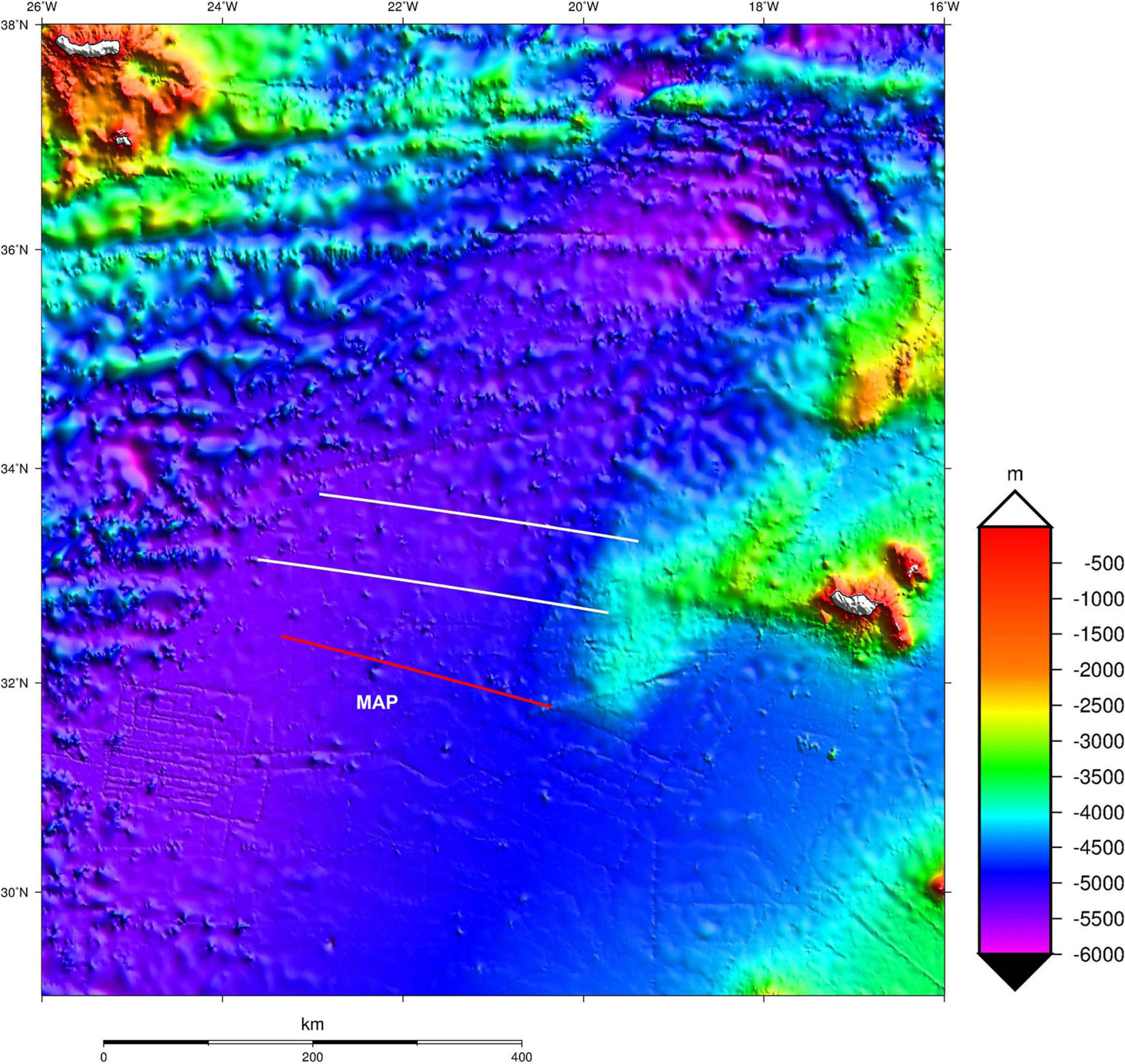
Figure 2. Location of the MAP. The red line shows the location of the SO profile inverted with the proposed method. White lines correspond to other MCS profiles acquired under the same seismic acquisition survey.
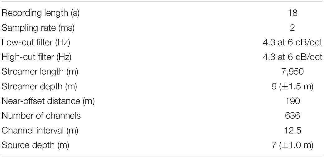
Table 1. Summary of the acquisition parameters of the MCS profiles acquired in the MAP.
The MCS profile was processed to image the fine-structure in the water column. Particular attention was given to mitigate the effect of the direct arrival and enhance shallow reflections while preserving true amplitudes by applying processing parameters that minimize amplitude and phase distortion. Different processing sequences would produce different results and impact the models predicted with the SO inversion. The detailed description of the processing sequence is presented in the following sub-section.
As collocated and contemporaneous direct measurements of temperature and salinity were not available, we used three vertical profiles of temperature and salinity (from two ARGO floats—ARGO, 4,660 and 44,909), profiling close to the acquisition period (in May 21 and May 31, 2006) and located in the surroundings of the SO section during the data acquisition (Figure 3). The ARGO profiles were used to infer the marginal (Figure 4) and joint distributions (Figure 5) of both ocean properties and were used as conditioning distributions for the stochastic sequential simulation and co-simulation of temperature and salinity models. We assume that the statistical properties of temperature and salinity measured by these floats hold for the location of the SO profile. According to the temperature and salinity measurements, three distinct water masses could be inferred: central Atlantic water; MOW; and Subarctic Intermediate Water, as described in Comas-Rodríguez et al. (2011). Low-frequency temperature and salinity background models were built using a global ocean dynamics model (CMEMS, 2016) for the dates of seismic acquisition (Figure 6). These two-dimensional sections are collocated with the MCS data but are smooth and low resolution. While the background temperature model shows a vertical trend of high temperature at shallower water depths and low temperature at deeper depths, the background salinity model follows the description above and considers the effect of the MOW (i.e., a saltier water layer) around 1,125 m of water depth.
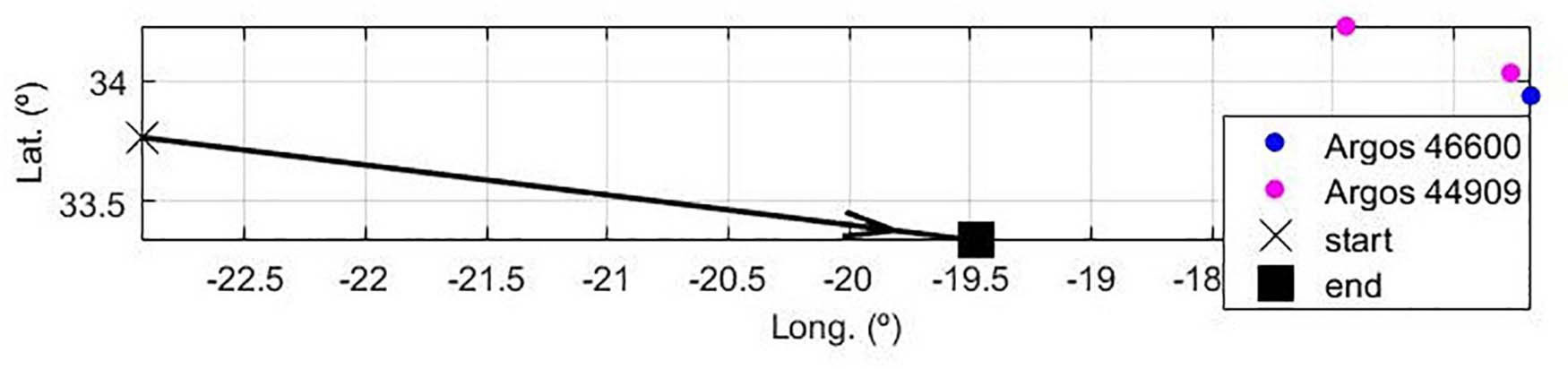
Figure 3. Relative location of the SO seismic profile and the two ARGO floats used for the seismic oceanography inversion.
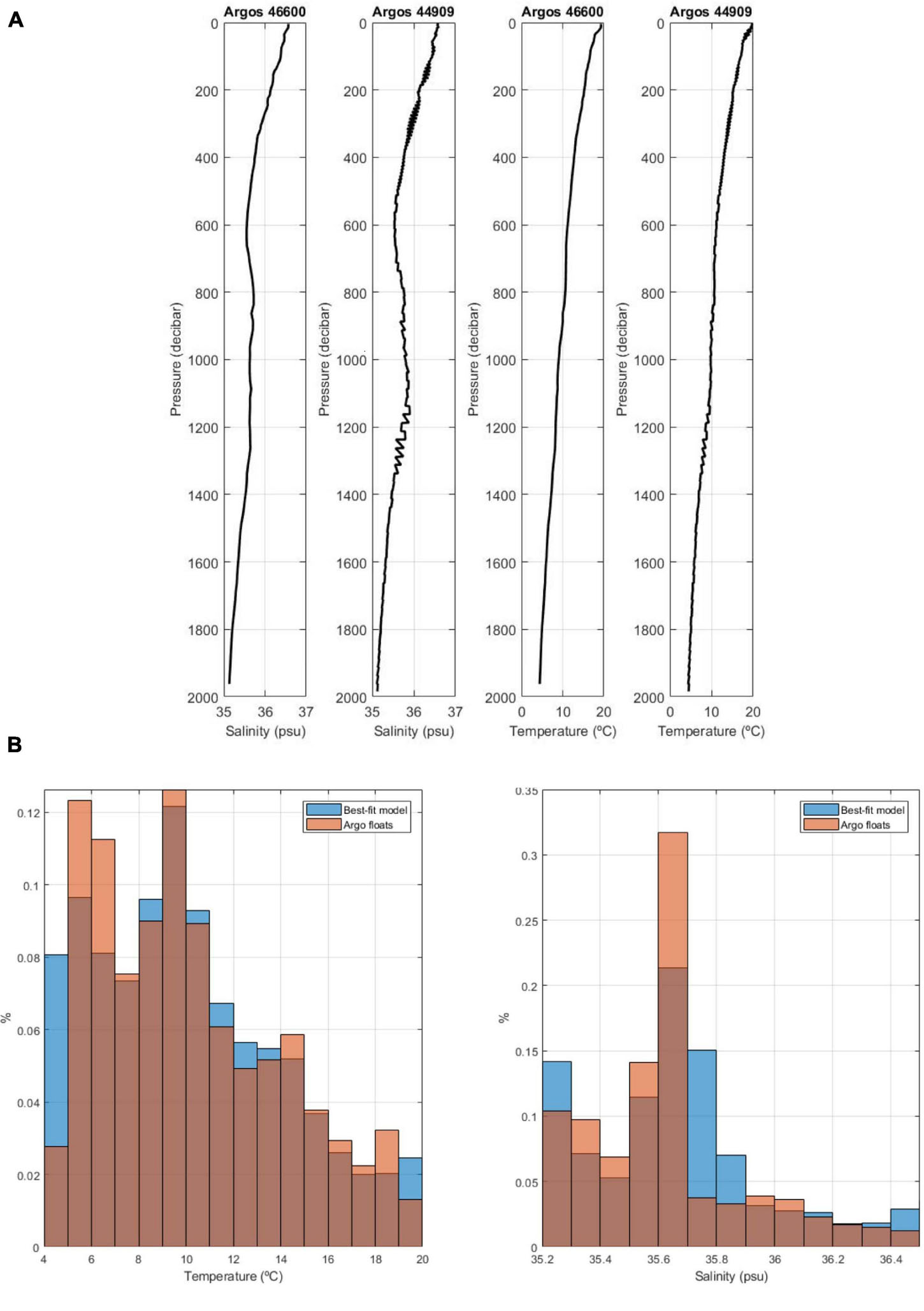
Figure 4. (A) ARGO profiles showing the measured temperature and salinity vs. pressure. (B) Comparison between histograms inferred from the temperature and salinity measured by the ARGO floats and the best-fit inverse models.
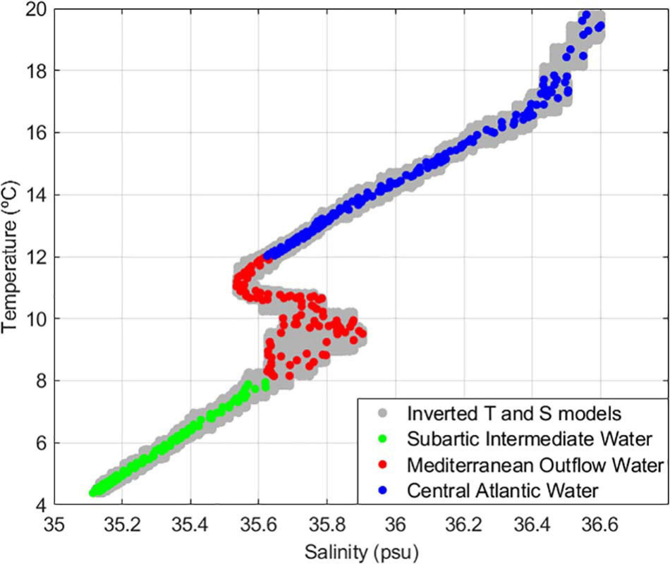
Figure 5. Joint distribution of temperature vs. salinity. Colored markers represent direct measurements from two ARGO floats and were used as training dataset for the Bayesian classification; pair of best-fit inverse models retrieved at the end of the inversion procedure are colored in gray.
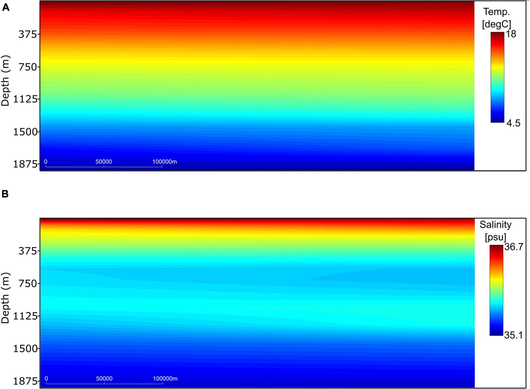
Figure 6. Background models of (A) temperature and (B) salinity extracted from the large-scale dynamics ocean model.
The processing sequence (Figure 7) included data resampling and recording length reduction to comprise data exclusively above the seafloor. Bad traces, both due to poor signal-to-noise ratio or bad readings, were edited and those unrecoverable were removed from the dataset. The direct arrival was tackled by applying a horizontal median filter with adaptive amplitude subtraction, similar to ocean bottom seismometers data processing (Duncan and Beresford, 1995). This kind of amplitude subtraction aims at minimizing the effects on the resulting amplitudes. This process was performed sequentially in a four-step approach (Figure 8): first, field records were flattened using a linear moveout correction with a constant velocity of 1,500 m/s (Figure 8A); the flattened records were doubled to avoid edge effects when applying a median filter (Figure 8B); a horizontal median filter was applied to those records to preserve horizontal coherent reflection (Figure 8C). Finally, the resulting record was subtracted to the doubled flatten record (Figure 8E) to eliminate the effect of the direct arrivals and keep reflections in the records (Figure 8F). The filtered gather, after applying a normal moveout (NMO) correction with a constant velocity of 1,500 m/s, is shown in Figure 8G where the reflections within the water column around 500 ms are enhanced.
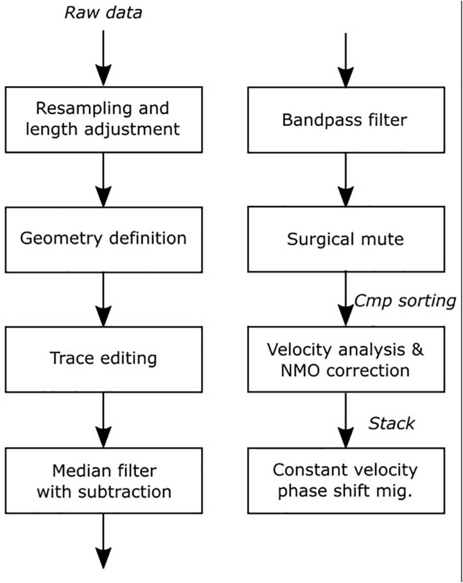
Figure 7. Seismic processing flow applied to the SO profile to enhance the reflections within the water column and in particular the shallow part of the section.
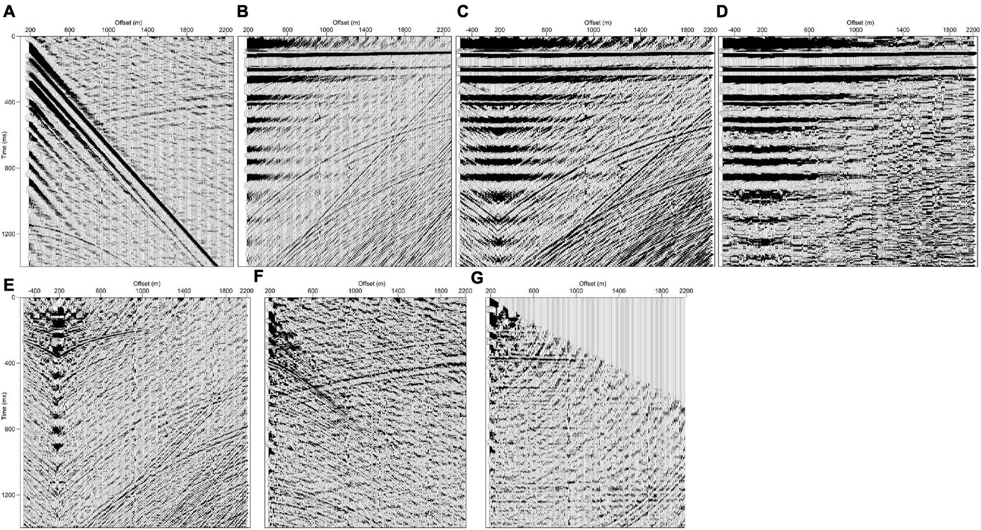
Figure 8. (A) An illustrative field seismic record. Echo from the previous shot is very clear. Shallow reflections from the water layer are obscured by the very strong direct arrival; (B) field record after linear moveout; (C) doubling the short offsets and merging to build a shot gather that will mitigate the border effects of the median filter; (D) after applying the median filter with 11 traces; (E) same as (C) after subtraction of the median filter shown in (D); (F) field record [as shown in (A)], after the full processing sequence of horizontal median filter with subtraction to attenuate the energy from the direct wave in the water; (G) processed record after NMO correction at 1,500 m/s (50% stretch mute allowed).
The second part of the processing sequence comprises band-pass filtering between 10 and 80 Hz, and surgical mutes to remove bursts of energy at the smallest offsets (Pinheiro et al., 2010). True amplitude recovery was applied to compensate spherical divergence. A detailed velocity analysis was performed along the MCS profile. The resulting velocity field was used in the normal moveout correction of the records. After CMP sorting, the CMP gathers were stacked considering all offsets. Finally, a constant velocity (1,500 m/s) phase-shift migration (Stolt, 1978) and time-to-depth conversion were carried out using the same constant velocity model.
Due to computational constraints, the MCS profile was processed in swaths of 400 field records, with an overlap of 50 records. This computational limitation results in the vertical stripping observed in the final time migrated section, which also affect the inverted temperature and salinity models (Figure 9). All sections are plotted in the depth domain to ease interpretation by assuming an average P-wave velocity of 1,500 m/s. However, the inversion of the SO section was performed in the time domain (i.e., prior to depth conversion).
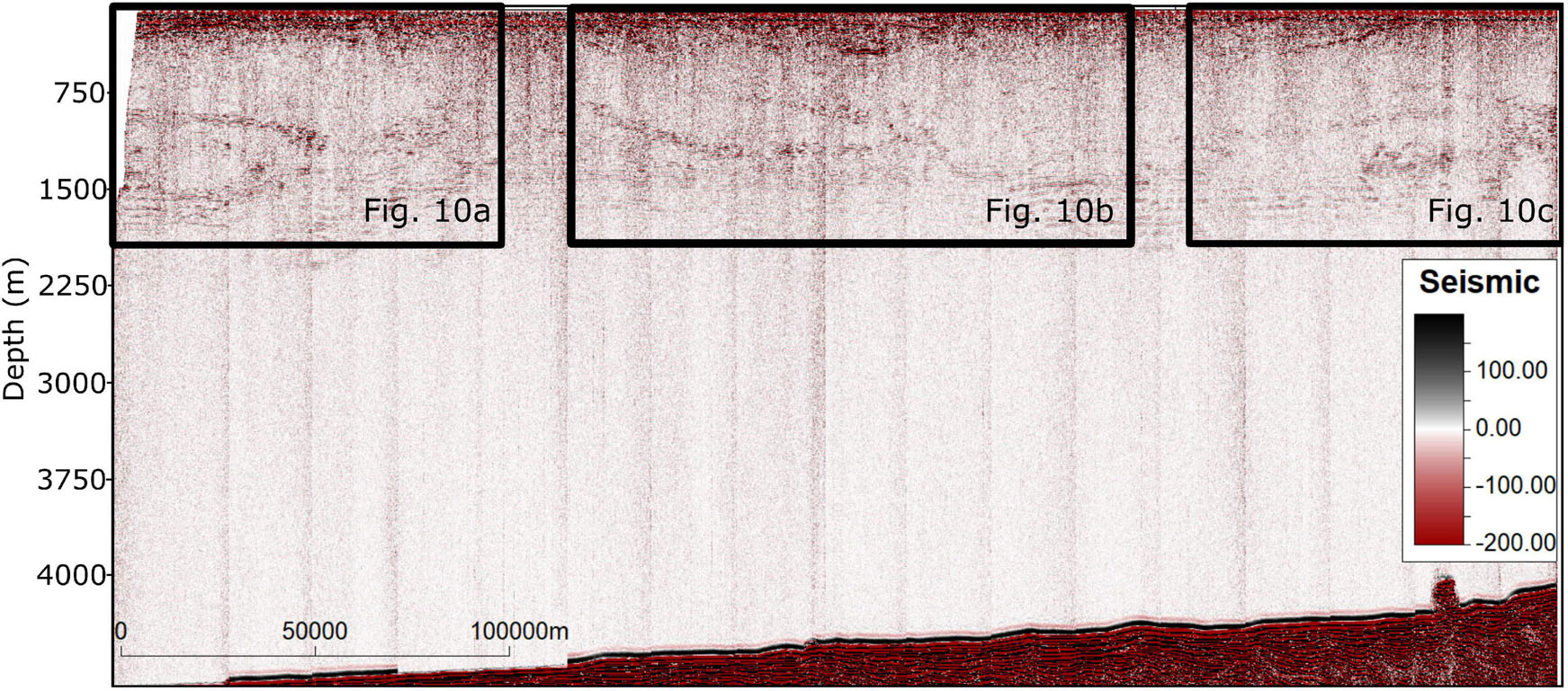
Figure 9. Migrated seismic profile. Black boxes represent the locations of the zoom-ins shown in Figure 10.
A preliminary interpretation of the SO profile allows its vertical division in two layers: the top one, down to approximately 1,875 m, comprises bright and coherent reflections with different seismic signatures and dips; the bottom one, below this depth, which is relatively reflection-free maybe due to the relatively homogeneous North Atlantic Deep Water. For this reason, only the top layer of the SO profile was considered for the geostatistical inversion (i.e., from 0 to 2.5 s in TWT).
The top layer shows the presence of an eddy at depths where Meddies are typically expected 600–1,500 m (Figure 10A). A smaller lenticular feature is also observed at shallow depths (around 750 m) that could be associated with the transition to Mediterranean waters or a secondary feature associated with that eddy (Figure 10B). Oblique reflections between 750 and 2,250 m might be related to oceanic fronts within the MOW or an inclined eddy of smaller dimensions as imaged in Tang et al. (2020). A possible double diffusion phenomenon can be detected by the continuous, parallel and bright reflections at approximately 1,500 ms for almost all the profile (Figure 10C). Double diffusion generates staircase thermohaline structure. The seismic signature of this oceanic structure has already been observed and investigated in the area near the Lesser Antilles in the Caribbean Sea (e.g., Fer et al., 2010) and in the Gulf of Cadiz associated to Mediterranean Outflow Water eddies (e.g., Biescas et al., 2008).
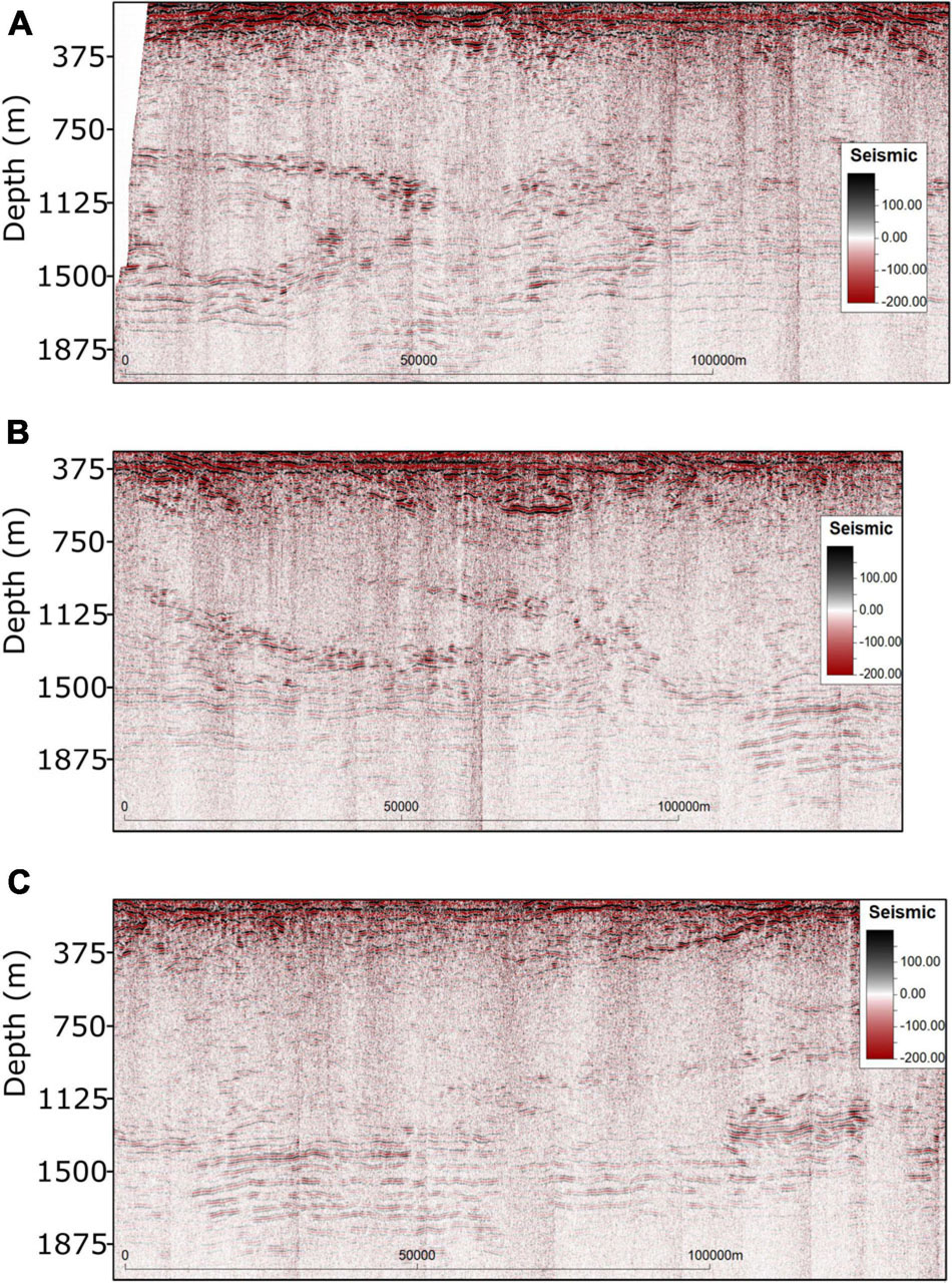
Figure 10. Close-up of: (A) the eddy interpreted in the Western part of the profile; (B) elliptical shallow feature and oblique reflection within the MOW; and (C) bright continuous seismic reflections interpreted as possible double diffusion.
The geostatistical SO inversion ran with six iterations, where at each iteration thirty-two pairs of temperature and salinity models were generated using direct sequential simulation (Soares, 2001) and direct sequential co-simulation with joint probability distributions (Horta and Soares, 2010). The stochastic sequential simulation and co-simulation were conditioned to the histograms and bi-histograms from Figures 4, 5, respectively. Since the ARGO floats were not located along the seismic profile, no spatial conditioning was considered. Vertical variograms for each property were modeled from both ARGO floats while the horizontal variogram was modeled directly on the seismic amplitudes. This is a conventional approach in seismic reservoir characterization and often results in overestimation of the horizontal ranges of the variogram model (Azevedo and Soares, 2017). The objective function (Eq. 4) used to drive the inversion is based on the mismatch between synthetic and real seismic traces used for the inversion and the deviation of each realization of temperature and salinity from the background models shown in Figure 6.
The synthetic SO data computed from the pointwise average temperature and salinity models generated during the last iteration is shown in Figure 11. These data reproduce the location of the main oceanographic features as interpreted from the observed data as well as their amplitude content. As expected, the synthetic SO data calculated from these models is less noisy than the observed seismic (e.g., Avseth et al., 2005) and, consequently, increases the spatial continuity of the seismic reflections at the bottom part of the section (∼1,500 m). Iterative geostatistical seismic inversion methods are known for the ability to remain unmatched in noisy areas of the observed data (Azevedo and Soares, 2017). This effect is illustrated by the lack of vertical artifacts in the synthetic data. To illustrate the local convergence of the synthetic data, Figure 11C shows the trace-by-trace S between true and inverted SO data.
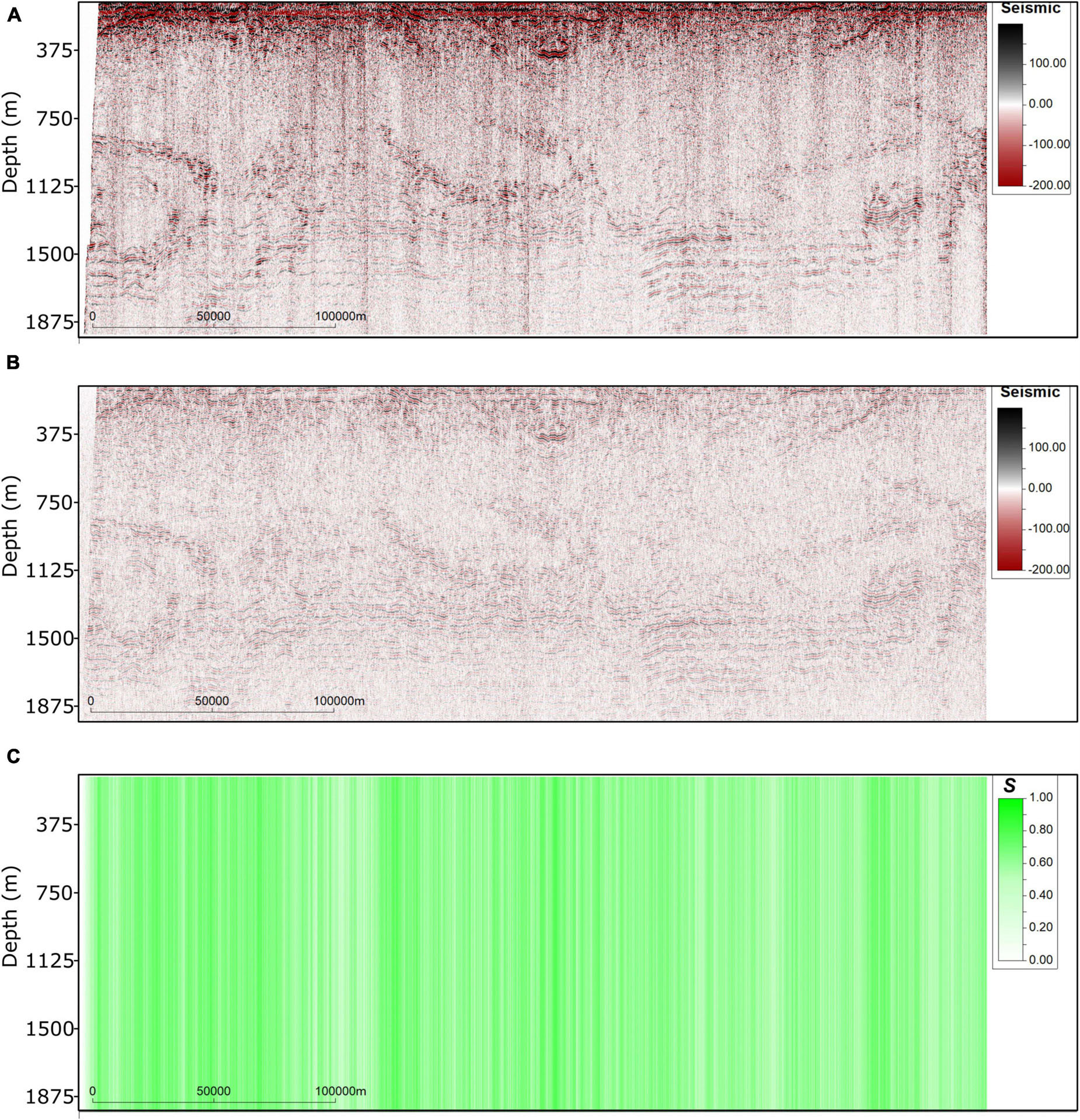
Figure 11. (A) Observed SO data used in the inversion; (B) synthetic SO data computed from the pointwise mean temperature and salinity models generated during the last iteration; (C) trace-by-trace S between (A,B).
The inverted temperature and salinity models (Figure 12) capture the oceanic features of interest at finer scale when compared with the observed SO data. This effect is related to the use of geostatistical simulation as model perturbation technique, the geostatistical simulation fills-in the frequency band related to high-frequencies (Azevedo and Soares, 2017). Modeling oceanographic features at these scales is not possible with either deterministic seismic inversion methods or conventional interpolation techniques of direct observations of the ocean properties as represented by CTDs or XBTs. This is one of the main benefits of using geostatistical seismic inversion methods. These models show the filamentation structures around the eddie’s core and in particular the warm intrusions around the homogenous nucleus. The use of background temperature and salinity models (Figure 6) allows reproducing the expected large-scale vertical distribution of both properties as interpreted from the global ocean models.
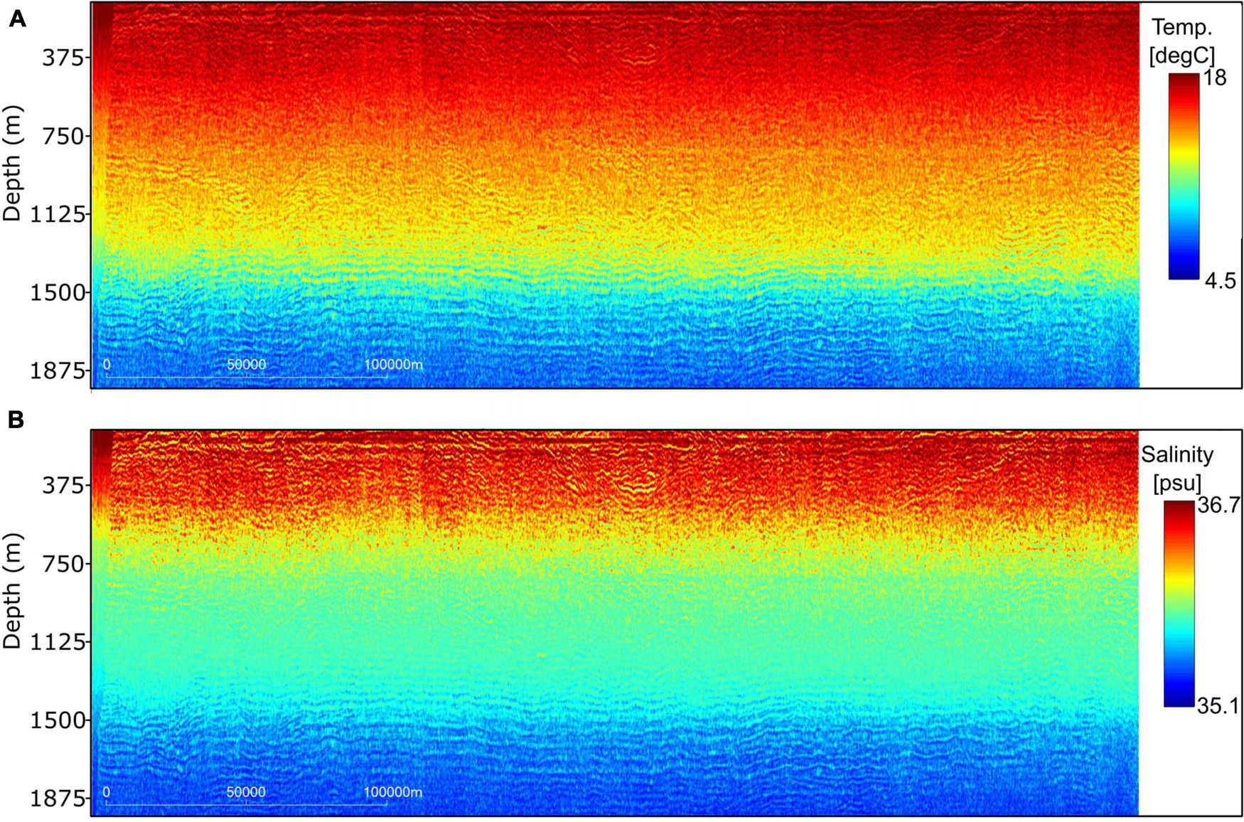
Figure 12. Pointwise mean model of the set of inverted (A) temperature and (B) salinity models generated during the last iteration of the geostatistical inversion.
Additionally, the benefit of using geostatistical inversion methods is related to the ability to assess the uncertainty associated with the model predictions. Figure 13 shows the pointwise variance of temperature and salinity computed from the ensemble of models generated for each property during the last iteration of the inversion procedure. It is interesting to discuss the spatial distribution pattern of these models. As temperature is the main contributor for the existence of reflection coefficients (Ruddick et al., 2009; Sallarès et al., 2009) the spatial uncertainty (i.e., the variance) is smaller in regions where the observed SO data exhibits coherent seismic reflections (i.e., above approximately 375 m and below 1,500 m). On the other hand, the region of lower variance for salinity, between the 750 and 1,125 m, matches the depths associated with the saltier layer as observed in the background model (Figure 6). The reason for this phenomenon still needs to be further investigated but might be related to: (i) the differences in signal-to-noise ratio in different parts of the seismic section; (ii) the local influence of the background models.
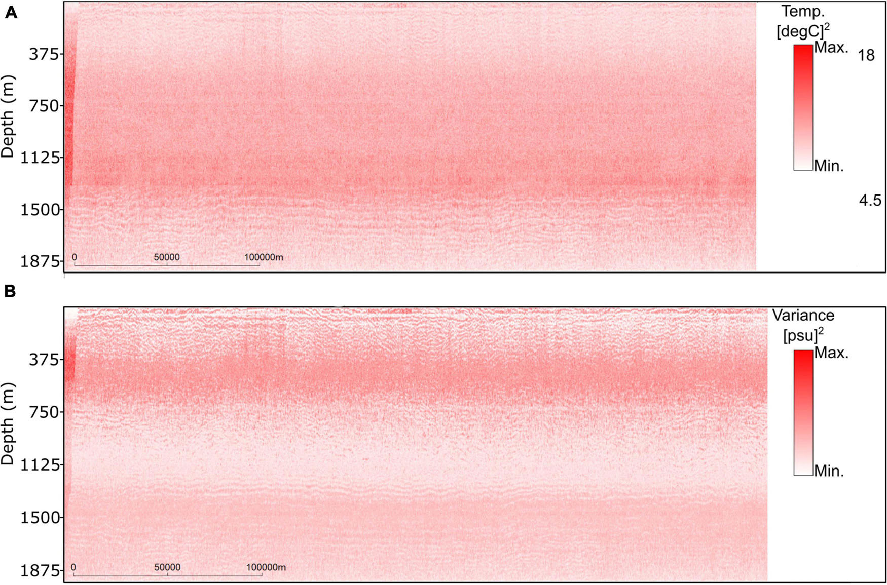
Figure 13. Pointwise variance model of the set of inverted (A) temperature and (B) salinity models generated during the last iteration of the geostatistical inversion.
When contemporaneous direct measurements of temperature or salinity along the SO profile are available, one could assess the local performance of the inversion by retaining one observation out of the conditioning data and comparing the inverted traces with the observed data (i.e., a blind-well test in subsurface modeling). In this application example we compare the depth trend of the inverted two-dimensional sections of temperature and salinity of all the realizations generated during the last iteration of the inversion with the vertical one-dimensional profiles acquired by the ARGO floats (Figure 14). Note that the ARGO floats are not used to spatially constrain the inversion. In this simple exercise we aim at evaluating if the vertical trend of both properties is reproduced. As expected the direct measurements are not exactly reproduced but we consider the reproduction of the main trends to be a positive result. To illustrate the potential of geostatistical seismic inversion methods we used the ensemble of pairs of temperature and salinity models generated during the last iteration to generate two-dimensional sections of probability of occurrence of different water masses. First each pair of models was classified into three distinct water masses using Bayesian classification. The a priori probabilities were inferred from the ARGO floats profiles, which were used as a training dataset (Figure 5). After classification of each pair, the ensemble of 32 models was used to compute the probability of occurrence of each water type (Figure 15). The resulting probability sections agree with the overall knowledge of this oceanic basin and with previous results obtained using exclusively large-scale oceanographic observations (Comas-Rodríguez et al., 2011). It is relevant to highlight that the order relationship of the different water masses (i.e., the Central Atlantic Water above the MOW above of the Subarctic Intermediate Water) is reproduced in the probability models, but it is not imposed by any other information rather than the SO data and the background models. As expected the regions of higher uncertainty are located at the boundaries of each water mass.
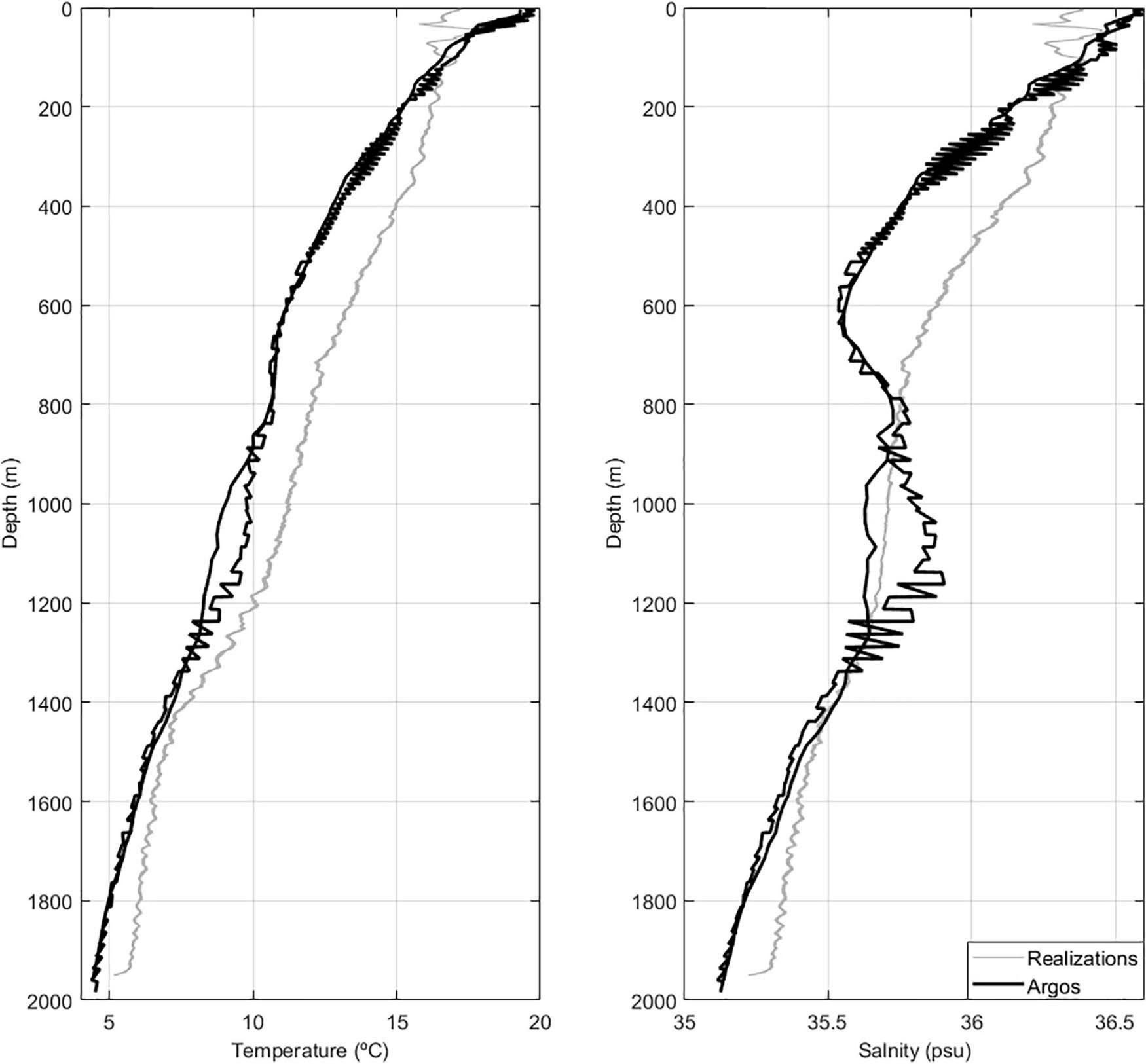
Figure 14. Comparison between the temperature and salinity vertical profiles measured at the ARGO floats locations (Figure 3) and the average vertical profile of temperature and salinity for all the thirty-two realizations generated during the last iteration of the geostatistical inversion.
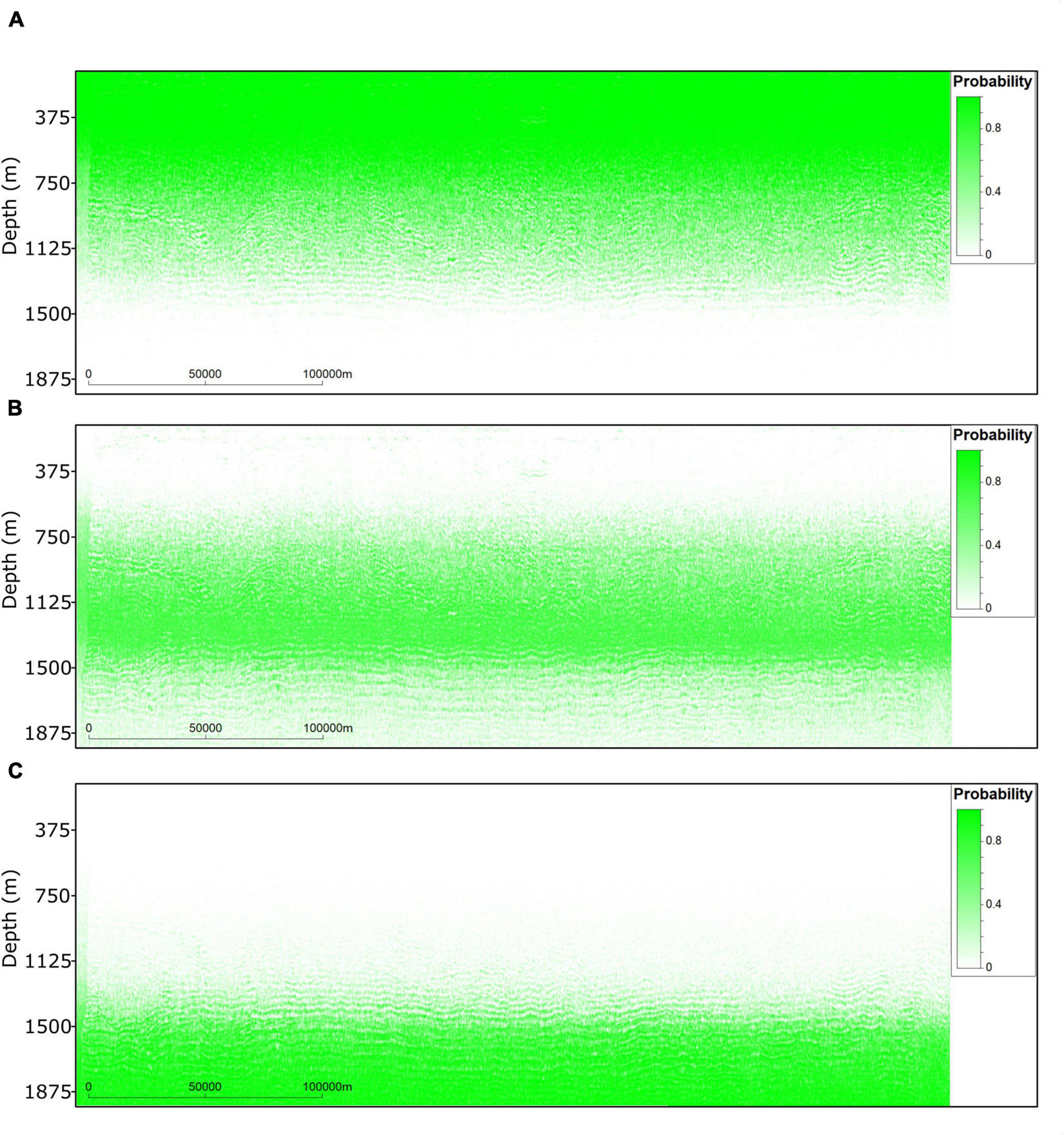
Figure 15. Probability of occurrence of: (A) Central Atlantic Water; (B) Mediterranean Outflow Water; (C) Subarctic Intermediate Water. Probability models calculated from the classification of the thirty-two temperature and salinity models generated during the last iteration of the inversion using the training data shown in Figure 5.
This paper presents the first seismic oceanography images of the Madeira abyssal plain region. The work focuses on two main aspects: (i) the introduction of a simple but efficient way to mitigate the effect of the direct arrival in the data; and (ii) the development of a geostatistical SO inversion that can be used when contemporaneous and collocated direct measurements are not available. The interpretation of the inverted models from an oceanographic perspective is limited, as it would benefit from the processing and inversion of the other two adjacent SO sections.
The processing sequence applied to these data was able to effectively attenuate the effect of the direct wave, revealing reflections in the first few hundred meters below the sea surface (Figure 10). The time-migrated section clearly shows fine-scale structure down to 2,000 m, below this depth the SO data shows no reflection. The upper part of the section exhibits a series of interesting oceanographic features that might be interpreted as eddies associated with the MOW and as double diffusive phenomena. However, these features need to be further explored to provide insights about the complex dynamics of the study area (Figure 10). The detailed interpretation of these oceanographic features will be performed after inverting the neighbor SO profiles existing in the region.
The processed time-migrated section was inverted using the proposed geostatistical SO inversion. We show how this inversion technique can be applied when no direct and contemporaneous observations of the ocean are available. We leverage common models of large-scale ocean dynamics and existing vertical profiles of the ocean properties measured by ARGO floats. This method was proved to be a useful tool to characterize sub-mesoscale oceanic features and has demonstrated a potential to invert for temperature and salinity. From the inverted models we also propose Bayesian classification of water masses. The probability of occurrence of the different water masses along the profile clearly agrees with the known vertical distribution (Figure 15).
As a final remark, it is worthwhile to highlight that the ensemble of inverted temperature and salinity fields generated at the last iteration still exhibits large variability (Figure 14). While this uncertainty is related to the lack of knowledge about the system under investigation (i.e., the ocean properties), it may be reduced and better predictions can be obtained by including additional constraints from other oceanographic variables (e.g., density, water column stability) during the inversion procedure. This approach would increase the reliability of the inverted models.
The original contributions presented in the study are included in the article/supplementary material, further inquiries can be directed to the corresponding author/s.
LA conceptualized and implemented 50% of the geostatistical SO inversion and wrote of the manuscript. LM conceptualized and supervised the SO processing data and wrote part of the manuscript. FT implemented 50% of the geostatistical SO inversion, ran the inversion on the application example, and wrote the manuscript. RT applied the SO processing flow. ÁP contributed for the preliminary interpretation of the results from an oceanographic point of view and wrote the manuscript. All authors contributed to the article and approved the submitted version.
The authors declare that the research was conducted in the absence of any commercial or financial relationships that could be construed as a potential conflict of interest.
All claims expressed in this article are solely those of the authors and do not necessarily represent those of their affiliated organizations, or those of the publisher, the editors and the reviewers. Any product that may be evaluated in this article, or claim that may be made by its manufacturer, is not guaranteed or endorsed by the publisher.
We gratefully acknowledge the support of the CERENA (strategic project FCT-UIDB/04028/2020). We would also like to thank EMEPC for acquiring and making this seismic profile available, CGG for the donation of Hampson-Russell used to extract the wavelet from the seismic oceanography data, Schlumberger for the donation of academic licenses of Petrel®, and Parallel Geoscience Corporation for SPW 4.0 used for the processing of the seismic data. These direct measurements of temperature and salinity were collected and made freely available by the International ARGO Program and the national programs that contribute to it (http://www.argo.ucsd.edu and http://argo.jcommops.org). The ARGO Program is part of the Global Ocean Observing System. This study has been conducted using E.U. Copernicus Marine Service Information. We are also grateful to the two reviewers for the detailed and extensive review of the original manuscript.
Argo (2000). Argo Float Data and Metadata from Global Data Assembly Centre (Argo GDAC). SEANOE. doi: 10.17882/42182
Avseth, P., Mukerji, T., and Mavko, G. (2005). Quantitative Seismic Interpretation. Cambridge: Cambridge University Press.
Azevedo, L., Huang, X., Pinheiro, L. M., Nunes, R., Caeiro, M. H., Song, H., et al. (2018). Geostatistical inversion of seismic oceanography data for ocean salinity and temperature models. Math. Geosci. 50, 477–489. doi: 10.1007/s11004-017-9722-x
Azevedo, L., Nunes, R., Correia, P., Soares, A., Guerreiro, L., and Neto, G. S. (2015). Integration of well data into geostatistical seismic amplitude variation with angle inversion for facies estimation. Geophysics 80, M113–M128.
Azevedo, L., and Soares, A. (2017). Geostatistical Methods for Reservoir Geophysics, 1st Edn. Salmon Tower Building, NY: Springer International Publishing.
Barbosa Aguiar, A., Peliz, A., and Carton, X. (2013). A census of Meddies in a long-term high-resolution simulation. Progr. Oceanogr. 116, 80–94. doi: 10.1016/j.pocean.2013.06.016
Barbosa Aguiar, A. C., Peliz, A. J., Cordeiro Pires, A., and Le Cann, B. (2011). Zonal structure of the mean flow and eddies in the Azores Current system. J. Geophys. Res. 116.
Biescas, B., Ruddick, B. R., Nedimovic, M. R., Sallarès, V., Bornstein, G., and Mojica, J. F. (2014). Recovery of temperature, salinity, and potential density from ocean reflectivity. J. Geophys. Res. Oceans 119, 3171–3184. doi: 10.1002/2013JC009662
Biescas, B., Sallarès, V., Pelegrí, J. L., Machín, F., Carbonell, R., Buffett, G., et al. (2008). Imaging meddy finestructure using multichannel seismic reflection data. Geophys. Res. Lett. 35:11.
Blacic, T. M., Jun, H., Rosado, H., and Shin, C. (2016). Smooth 2-D ocean sound speed from Laplace and Laplace-Fourier domain inversion of seismic oceanography data. Geophys. Res. Lett. 43, 1211–1218. doi: 10.1002/2015GL067421
Bornstein, G., Biescas, B., Sallarès, V., and Mojica, J. F. (2013). Direct temperature and salinity acoustic full waveform inversion. Geophys. Res. Lett. 40, 4344–4348. doi: 10.1002/grl.50844
Bortoli, L. J., Alabert, F., Haas, A., and Journel, A. G. (1993). “Constraining stochastic images to seismic data,” in Geostatistics Troia’92, ed. A. Soares (Dordrecht: Kluwer), 325–337.
Bosch, M., Mukerji, T., and González, E. F. (2010). Seismic inversion for reservoir properties combining statistical rock physics and geostatistics: A review. Geophysics 75:75A165. doi: 10.1190/1.3478209
Chhun, C., and Tsuji, T. (2020). Sound speed of thermohaline fine structure in the Kuroshio Current inferred from automatic sound speed analysis. Expl. Geophys. 51, 581–590. doi: 10.1080/08123985.2020.1736548
CMEMS (2016). Global Ocean 1/12° Physics Analysis and Forecast Updated Daily. Available online at: https://sextant.ifremer.fr/record/eec7a997-c57e-4dfa-9194-4c72154f5cc5/
Comas-Rodríguez, I., Hernández-Guerra, A., Fraile-Nuez, E., Martínez-Marrero, A., Benítez-Barrios, V. M., Pérez-Hernández, M. D., et al. (2011). The Azores Current System from a meridional section at 24.5°W. J. Geophys. Res. 116:C09021. doi: 10.1029/2011JC007129
Dagnino, D., Sallarès, V., Biescas, B., and Ranero, C. R. (2016). Fine-scale thermohaline ocean structure retrieved with 2-D prestack full-waveform inversion of multichannel seismic data: Application to the Gulf of Cadiz (SW Iberia). J. Geophys. Res. Oceans 121, 5452–5469. doi: 10.1002/2016JC011844
Dagnino, D., Sallarès, V., and Ranero, C. R. (2018). Waveform-preserving processing flow of multichannel seismic reflection data for Adjoint-State Full-waveform inversion of ocean Thermohaline Structure. IEEE Trans. Geosci. Remote Sen. 56, 1615–1625. doi: 10.1109/TGRS.2017.2765747
Deutsch, C. V., and Journel, A. G. (1992). GSLIB: Geostatistical Software Library and User’s Guide. New York, NY: Oxford University Press.
Dickinson, A., White, N. J., and Caulfield, C. P. (2017). Spatial variation of diapycnal diffusivity estimated from seismic imaging of internal wave field, Gulf of Mexico. J. Geophys. Res. Oceans 122, 9827–9854. doi: 10.1002/2017jc013352
Duncan, G., and Beresford, G. (1995). Median filter behaviour with seismic data. Geophys. Prospect. 43, 329–345. doi: 10.1111/j.1365-2478.1995.tb00256.x
Fer, I., Nandi, P., Holbrook, W. S., Schmitt, R. W., and Páramo, P. (2010). Seismic imaging of a thermohaline staircase in the western tropical North Atlantic. Ocean Sci. 6, 621–631. doi: 10.5194/os-6-621-2010
Fortin, W. F. J., Holbrook, W. S., and Schmitt, R. W. (2017). Seismic estimates of turbulent diffusivity and evidence of nonlinear internal wave forcing by geometric resonance in the South China Sea. J. Geophys. Res. Oceans 122, 8063–8078. doi: 10.1002/2017jc012690
Gennert, M. A., and Yuille, A. L. (1988). “Determining the optimal weights in multiple objective function optimization,” in Proceedings of the Second International Conference on Computer Vision, (Tampa, FL), 87–89.
González, E. F., Mukerji, T., and Mavko, G. (2008). Seismic inversion combining rock physics and multiple-point geostatistics. Geophysics 73, R11–R21. doi: 10.1190/1.2803748
Grana, D., Lang, X., and Wu, W. (2017). Statistical facies classification from multiple seismic attributes: comparison between Bayesian classification and expectation-maximization method and application in petrophysical inversion. Geophys. Prospect. 65, 544–562. doi: 10.1111/1365-2478.12428
Grana, D., Mukerji, T., Dvorkin, J., and Mavko, G. (2012). Stochastic inversion of facies from seismic data based on sequential simulations and probability perturbation method. Geophysics 77, M53–M72. doi: 10.1190/geo2011-0417.1
Gunn, K. L., White, N., and Caulfield, C.-c. P (2020). Time-Lapse seismic imaging of oceanic fronts and transient lenses within South Atlantic Ocean. J. Geophys. Res. Oceans 125:e2020JC016293. doi: 10.1029/2020JC016293
Gunn, K. L., White, N. J., Larter, R. D., and Caulfield, C. P. (2018). Calibrated seismic imaging of eddy-dominated warm-water transport across the Bellingshausen Sea, Southern Ocean. J. Geophys. Res. Oceans 123, 3072–3099. doi: 10.1029/2018JC013833
Hardy, R., Jones, S., Hardy, D., and Hobbs, R. (2007). Seismic Oceanography: Processing Data From the Rockall Trough, West of Ireland. SEG Technical Program Expanded Abstracts. Tulsa, OK: Society of Exploration Geophysicists, 894–898.
Hobbs, R., Carbonell, R., Artale, V., Geli, L., Gutscher, M., Huthnance, J., et al. (2007). GO—Geophysical Oceanography: A New Tool to Understand the Thermal Structure and Dynamics of Oceans. Durham: Durham University.
Holbrook, W. S., Fer, I., Schmitt, R. W., Lizarralde, D., Klymak, J. M., Helfrich, L. C., et al. (2013). Estimating oceanic turbulence dissipation from seismic images. J. Atmospheric Oceanic Technol. 30, 1767–1788. doi: 10.1175/jtech-d-12-00140.1
Holbrook, W. S., Paramo, P., Pearse, S., and Schmitt, R. W. (2003). Thermohaline fine structure in an oceanographic front from seismic reflection profiling. Science 301, 821–824. doi: 10.1126/science.1085116
Horta, A., and Soares, A. (2010). Direct sequential co-simulation with joint probability distributions. Math. Geosci. 42, 269–292. doi: 10.1007/s11004-010-9265-x
Huang, X., Song, H., Bai, Y., Chen, J., and Liu, B. (2012). Estimation of seawater movement based on reflectors from a seismic profile. Acta Oceanol. Sin 31, 46–53. doi: 10.1007/s13131-012-0235-7
IOC, SCOR, and IAPSO (2010). The International Thermodynamic Equation of Seawater - 2010: Calculation and Use of THERMODYNAMIC PROPERTIES. INTERGOVERNMENTAL Oceanographic Commission, Manuals and Guides No. 56. Paris: UNESCO, 196.
Jones, S. M., Hardy, R. J. J., Hobbs, R. W., and Hardy, D. (2008). The new synergy between seismic reflection imaging and oceanography. First Break 26: 8010.
Jun, H., Cho, Y., and Noh, J. (2019). Trans-dimensional Markov chain Monte Carlo inversion of sound speed and temperature: application to yellow sea multichannel seismic data J. Mar. Syst. 197:103180. doi: 10.1016/j.jmarsys.2019.05.006
Kormann, J., Biescas, B., Korta, N., de la Puente, J., and Sallarès, V. (2011). Application of acoustic full waveform inversion to retrieve high-resolution temperature and salinity profiles from synthetic seismic data. J. Geophys. Res 116:C11039. doi: 10.1029/2011JC007216
Le Ravalec-Dupin, M., and Noetinger, B. (2002). Optimization with the gradual deformation method. Math. Geol. 34, 125–142.
Mahadevan, A. (2016). the impact of submesoscale physics on primary productivity of plankton. Ann. Rev. Mar. Sci. 8, 161–184. doi: 10.1146/annurev-marine-010814-015912
Marler, R. T., and Arora, J. S. (2010). The weighted sum method for multi-objective optimization: new insights Struct. Multidiscip. Optim. 41, 853–862. doi: 10.1007/s00158-009-0460-7
Mead, J. L. (2008). Parameter estimation: a new approach to weighting a priori information. J. Inverse Ill-posed Probl. 16, 175–193. doi: 10.1515/JIIP.2008.011
Minakov, A., Keers, H., Kolyukhin, D., and Tengesdal, H. C. (2017). Acoustic waveform inversion for ocean turbulence. J. Phys. Oceanogr. 47, 1473–1491. doi: 10.1175/jpo-d-16-0236.1
Padhi, A., Mallick, S., Fortin, W., Holbrook, W. S., and Blacic, T. M. (2015). 2-D ocean temperature and salinity images from pre-stack seismic waveform inversion methods: an example from the South China Sea. Geophys. J. Int. 202, 800–810. doi: 10.1093/gji/ggv188
Papenberg, C., Klaeschen, D., Krahmann, G., and Hobbs, R. W. (2010). Ocean temperature and salinity inverted from combined hydrographic and seismic data. Geophys. Res. Lett. 37:L04601.
Páramo, P., and Holbrook, W. S. (2005). Temperature contrasts in the water column inferred from amplitude-versus-offset analysis of acoustic reflections. Geophys. Res. Lett. 32:L24611. doi: 10.1029/2005GL024533
Pascual, A., Ruiz, S., Olita, A., Troupin, C., Claret, M., Casas, B., et al. (2017). Multiplatform experiment to unravel meso- and submesoscale processes in an intense front (AlborEx). Front. Mar. Sci. 4:39. doi: 10.3389/fmars.2017.00039
Pereira, P., Azevedo, L., Nunes, R., and Soares, A. (2019). The impact of a priori elastic models into iterative geostatistical seismic inversion. J. Appl. Geophys. 170:103850. doi: 10.1016/j.jappgeo.2019.103850
Pinheiro, L. M., Song, H., Ruddick, B., Dubert, J., Ambar, I., Mustafa, K., et al. (2010). Detailed 2-D imaging of the mediterranean outflow and meddies off W Iberia from multichannel seismic data. J. Mar. Syst. 79, 89–100. doi: 10.1016/j.jmarsys.2009.07.004
Richardson, P. L., Bower, A., and Zenk, W. (2000). A census of meddies tracked by floats. Prog. Oceanogr. 45, 209–250. doi: 10.1016/s0079-6611(99)00053-1
Ristow, J. P., Cordioli, J. A., Barão, M. V. C., Klein, A. H. F., and Barrault, G. F. G. (2017). “Development of methodological proceeding for seismic oceanography using legacy multi-channel seismic data of the oil and gas industry,” in Proceedings of the 2017 IEEE/OES Acoustics in Underwater Geosciences Symposium (RIO Acoustics), (Rio de Janeiro), 1–8. doi: 10.1109/RIOAcoustics.2017.8349710
Ruddick, B., Song, H. B., Dong, C. Z., and Pinheiro, L. (2009). Water column seismic images as maps of temperature gradient. Oceanography 22, 192–205. doi: 10.5670/oceanog.2009.19
Sallarès, V., Biescas, B., Buffett, G., Carbonell, R., Dañobeitia, J. J., and Pelegrí, J. L. (2009). Relative contribution of temperature and salinity to ocean acoustic reflectivity. Geophys. Res. Lett. 36:L00D06.
Sallarès, V., Mojica, J. F., Biescas, B., Klaeschen, D., and Gràcia, E. (2016). Characterization of the submesoscale energy cascade in the Alboran Sea thermocline from spectral analysis of high-resolution MCS data. Geophys. Res. Lett. 43, 6461–6468. doi: 10.1002/2016gl069782
Sambridge, M. (1999). Geophysical inversion with a neighbourhood algorithm-I. Searching a parameter space. Geophys. J. Int. 138, 479–494. doi: 10.1046/j.1365-246x.1999.00876.x
Sams, M., and Carter, D. (2017). Stuck between a rock and a reflection: a tutorial on low-frequency models for seismic inversion. Interpretation 5, B17–B27.
Segade, L. I. C., Gilcoto, M., Mercier, H., and Pérez, F. F. (2015). Quasi-synoptic transport, budgets and water mass transformation in the Azores–Gibraltar Strait region during summer 2009. Progress Oceanogr. 130, 47–64. doi: 10.1016/j.pocean.2014.09.006
Sen, M. K., and Stoffa, P. L. (1991). Nonlinear one dimensional seismic waveform inversion using simulated annealing. Geophysics 56, 1624–1638. doi: 10.1190/1.1442973
Soares, A., Diet, J. D., and Guerreiro, L. (2007). “Stochastic inversion with a global perturbation method,” in Proceedings of the Petroleum Geostatistics EAGE, (Houten: European Association of Geoscientists and Engineers), 10–14.
Song, H. B., Huang, X. H., Pinheiro, L. M., Song, Y., Dong, C. Z., and Bai, Y. (2012). “Inversion studies in seismic oceanography,” in Computational Methods for Applied Inverse Problems, Chap. 16, eds Y. Wang, A. G. Yagola, and C. Yang (Berlin, Boston: De Gruyter), 395–410. doi: 10.1515/9783110259056.395
Tang, Q., Gulick, S. P. S., Sun, J., Sun, L., and Jing, Z. (2020). Submesoscale features and turbulent mixing of an oblique anticyclonic eddy in the Gulf of Alaska investigated by marine seismic survey data. J. Geophys. Res. Oceans 125:e2019JC015393. doi: 10.1029/2019JC015393
Tang, Q., Hobbs, R., Zheng, C., Biescas, B., and Caiado, C. (2016). Markov Chain Monte Carlo inversion of temperature and salinity structure of an internal solitary wave packet from marine seismic data. J. Geophys. Res. Oceans 121, 3692–3709. doi: 10.1002/2016JC011810
Tang, Q., Tong, V. C. H., Hobbs, R. W., and Morales Maqueda, M. Á (2019). Detecting changes at the leading edge of an interface between oceanic water layers. Nat. Commun. 10:4674. doi: 10.1038/s41467-019-12621-8
Tang, Q., Xu, M., Zheng, C., Xu, X., and Xu, J. (2018). A locally generated high-mode nonlinear internal wave detected on the shelf of the northern South China Sea from marine seismic observations. J. Geophys. Res. Oceans 123, 1142–1155. doi: 10.1002/2017JC013347
Tarantola, A. (2005). Inverse Problem Theory and Methods for Model Parameter Estimation. Philadelphia: Society for Industrial and Applied Mathematics, 1–54.
Warner, M. (1990). Absolute reflection coefficients from deep Seismic reflections. Tectonophysics 173, 15–23. doi: 10.1016/0040-1951(90)90199-I
Wood, W. T., Holbrook, W. S., Sen, M. K., and Stoffa, P. L. (2008). Full waveform inversion of reflection seismic data for ocean temperature profiles. Geophys. Res. Lett. 35:L04608. doi: 10.1029/2007GL032359
Keywords: seismic oceanography, geostatistical inversion, temperature prediction, salinity prediction, ocean modeling, Madeira Abyssal Plain
Citation: Azevedo L, Matias L, Turco F, Tromm R and Peliz Á (2021) Geostatistical Seismic Inversion for Temperature and Salinity in the Madeira Abyssal Plain. Front. Mar. Sci. 8:685007. doi: 10.3389/fmars.2021.685007
Received: 24 March 2021; Accepted: 19 July 2021;
Published: 12 August 2021.
Edited by:
Kathy Gunn, University of Miami, United StatesReviewed by:
Alex Dickinson, Newcastle University, United KingdomCopyright © 2021 Azevedo, Matias, Turco, Tromm and Peliz. This is an open-access article distributed under the terms of the Creative Commons Attribution License (CC BY). The use, distribution or reproduction in other forums is permitted, provided the original author(s) and the copyright owner(s) are credited and that the original publication in this journal is cited, in accordance with accepted academic practice. No use, distribution or reproduction is permitted which does not comply with these terms.
*Correspondence: Leonardo Azevedo, TGVvbmFyZG8uYXpldmVkb0B0ZWNuaWNvLnVsaXNib2EucHQ=
Disclaimer: All claims expressed in this article are solely those of the authors and do not necessarily represent those of their affiliated organizations, or those of the publisher, the editors and the reviewers. Any product that may be evaluated in this article or claim that may be made by its manufacturer is not guaranteed or endorsed by the publisher.
Research integrity at Frontiers
Learn more about the work of our research integrity team to safeguard the quality of each article we publish.