Visualising the Uncertainty Cascade in Multi-Ensemble Probabilistic Coastal Erosion Projections

Future projections of coastal erosion, which are one of the most demanded climate services in coastal areas, are mainly developed using top-down approaches. These approaches consist of undertaking a sequence of steps that include selecting emission or concentration scenarios and climate models, correcting models bias, applying downscaling methods, and implementing coastal erosion models. The information involved in this modelling chain cascades across steps, and so does related uncertainty, which accumulates in the results. Here, we develop long-term multi-ensemble probabilistic coastal erosion projections following the steps of the top-down approach, factorise, decompose and visualise the uncertainty cascade using real data and analyse the contribution of the uncertainty sources (knowledge-based and intrinsic) to the total uncertainty. We find a multi-modal response in long-term erosion estimates and demonstrate that not sampling internal climate variability’s uncertainty sufficiently could lead to a truncated outcomes range, affecting decision-making. Additionally, the noise arising from internal variability (rare outcomes) appears to be an important part of the full range of results, as it turns out that the most extreme shoreline retreat events occur for the simulated chronologies of climate forcing conditions. We conclude that, to capture the full uncertainty, all sources need to be properly sampled considering the climate-related forcing variables involved, the degree of anthropogenic impact and time horizon targeted.

Introduction

Mean sea level, wave conditions, storm surges and tides are shaping coasts worldwide (Wong et al., 2014). These coastal drivers are altered by global and regional climate change, bringing additional uncertainty to present conditions that grows toward the end of the century and beyond (Kopp et al., 2017). The way this uncertainty propagates from different levels of radiative forcing in the form of emission and concentration scenarios (RCPs) through global and regional climate models (GCMs and RCMs, respectively), and coastal regional forcing and erosion models is primarily assessed using top-down approaches (Ranasinghe, 2016; Toimil et al., 2020a), which require bias correction and downscaling procedures (Zscheischler et al., 2018). Top-down approaches involve undertaking a sequence of steps through which information and uncertainty cascade from one step to the next, leading to an expansion of the envelope of uncertainty, widely referred to as the cascade of uncertainty (Mitchell and Hulme, 1999; Wilby and Dessai, 2010) in the literature.

When it comes to develop coastal erosion projections, the uncertainty that arises from top-down approaches can be classified as intrinsic or knowledge-related (Toimil et al., 2020a). Intrinsic uncertainty is inherent to the climate change problem and irreducible (Giorgi, 2010) and includes uncertainty in emission scenarios and in the internal variability of the climate system. Conversely, knowledge uncertainty, which is said not to exist in the “real world” (Mankin et al., 2020), is rooted in our imperfect knowledge of atmospheric, biogeochemical, physical, dynamic and coastal processes and could be decreased by advancing science understanding and increasing computational resources. Knowledge uncertainty comprises concentration scenario uncertainty, GCM–RCM uncertainty, bias uncertainty, downscaling uncertainty, and (epistemic) coastal erosion model (CEM) uncertainty. Such uncertainty sources can dominate one another (Giorgi, 2010) and their importance depends on many factors that encompass the climate-related variable, the time horizon of the projection, the region, and the geographic scale (Hawkins and Sutton, 2009; Fernández et al., 2019).

It will never be possible to quantify very accurately the likelihood that future climate change will reach a particular magnitude, although some quantitative bounds can be assessed and potentially narrowed (Sutton, 2019). And even when uncertainty is large and irreducible and hampers communication, its characterisation remains the means to effective risk-informed decision-making (Mankin et al., 2020). To date, there have been many attempts to address uncertainty in climate projections, but little attention has been really paid to impacts and risks (IPCC, 2013, 2018), which require considering at least two important aspects that could bring additional challenges. Risk assessment seeks to account for the full range of potential unwanted or “bad” outcomes even when they are very uncertain (and very unlikely) (Sutton, 2019). The second aspect is associated with practical and conceptual barriers in how to approach uncertainty sampling across the entire top-down approach. Existing studies limit exploration to knowledge uncertainty and single dimensions, involving one or two steps in the top-down approach, for example, by considering different representative concentration pathways or RCPs, GCM, or GCM–RCM ensembles with a single realisation, a variation range of mean sea-level rise (SLR), or CEM ensembles (Toimil et al., 2020a). Accounting for these uncertainty sources in an aggregated manner, however, would help to identify what is the step in the top-down process contributing the most and where to focus efforts to reduce uncertainty. Internal variability uncertainty, which is due to the natural variations in the climate system, by contrast cannot be reduced and has been demonstrated to be large and persistent, having the potential to impoverish decision-making if disregarded (e.g., Mankin et al., 2020). In the same manner different GCMs and RCMs give different responses about future climate, so does different realisations of the same GCMs or RCMs (under the same assumptions) due to their stochastic nature. This noise arisen from internal variability can be a very valuable source of information for the assessment of coastal erosion, where the chronology of the climate-related forcing conditions could be determinant, especially on short-term timescales (Toimil et al., 2017).

Just as important as it is considering the cascade of uncertainty is to visualise it, and this is crucial because visualisation is usually the prelude to understanding. However, to our knowledge, very few studies to date have tried to visualise this cascade using real data, all of which focused on climate variables. For instance, Hawkins (2014) pioneered the visualisation of the uncertainty cascade in global mean surface temperature projections considering three pyramid levels (RCPs–GCMs-realisations). Following the same visualisation, Swart et al. (2015) analysed of the influence of internal variability on Arctic sea-ice extent (RCPs–GCMs-realisation) and, more recently, Fernández et al. (2019) presented a research work on seasonal precipitation and temperature changes and their dependence on GCMs and RCMs, realisations, emission scenarios or RCPs, and resolution. While studies on projections of coastal impacts and, in particular, of coastal erosion, have shown progress in the quantification of the relative contribution of uncertainty dimensions to the total uncertainty (e.g., Le Cozannet et al., 2019; Athanasiou et al., 2020), they mainly focus on the application of variance-based decomposition methods and mostly limit the top-down approach-related sources of uncertainty considered to RCPs, SLR, and CEMs, and do not provide neither a conception nor a visualisation of the full cascade.

In this paper, we develop coastal erosion projections following each of the steps of the top-down procedure and sampling the associated knowledge and intrinsic uncertainty. We decompose and factorise the cascade of uncertainty going from RCPs down to future coastal erosion estimates. Our approach combines the fully implementation of probabilistic SLR projections and dynamic projections of waves and storm surges in an ensemble of two CEMs for different RCPs and GCMs, including bias correction and the hybrid downscaling of waves to nearshore. In addition, we sample uncertainty in climate variability by generating thousands of synthetic multivariate time series of projected nearshore waves and storm surges, leading to chronologies different from the dynamic projections’ original realisation. Using a real beach as an illustration and looking at long-term shoreline recession and non-stationary extreme retreat events, we analyse the dependence of far-future coastal erosion projections on RCPs and GCMs, climate variability, SLR percentiles, and CEMs.

The paper is structured as follows. Section “Study Area” provides a brief description of the study area where the analysis is performed. Section “Development of Coastal Erosion Projections” describes the approach proposed for the development of coastal erosion projections. Section “Visualisation and Communication of Uncertainty in Coastal Erosion Projections” analyses uncertainty in coastal erosion projections and discusses ways of visualisation. Finally, section “Conclusion” provides some concluding remarks.

Study Area

The analysis is performed in San Lorenzo Beach, a pocket urban beach located in Gijon (Asturias), northern Spain. It has a macrotidal semidiurnal regime (2–5 m of spring tidal range) and fine (0.2–0.3 mm) quartz sand. The most energetic waves come from the Northwest to the North-Northwest sectors. During extreme weather events, these waves can reach up significant wave heights of 10 m and peak periods of 20 s. San Lorenzo response to coastal climate forcing is cross-shore dominated as has negligible alongshore gradients in longshore sediment transport and does not experience significant rotation. It has homogenous grain size and composition along its whole cross section and has a constant berm height along its length. Toimil et al. (2017) derived these parameters from field surveys.

Development of Coastal Erosion Projections

We develop long-term multi-ensemble probabilistic coastal erosion projections for the period 2081–2100 in San Lorenzo Beach following the steps of the top-down approach to sufficiently quantify the associated uncertainty. Such steps are shown in Figure 1. We first compile dynamic projections of waves and storm surges developed for 2 RCPs (RCP4.5 and RCP8.5, box A) and 6 GCMs each (box b1). In a second step, we correct their bias (box b2) and downscale wave projections to the coast using a hybrid approach that combines statistical and numerical modelling and incorporates the effects of projected mean sea level on nearshore waves (box b3). We generate 1,000 synthetic multivariate time series of GCM-driven projected wave conditions and storm surges (box b4). Additionally, we obtain 3 SLR trajectories corresponding to three percentiles from probabilistic local SLR projections for the radiative forcings RCP4.5 and RCP8.5, and reconstruct the astronomical tide (boxes c2, D, respectively). Finally, we apply 2 CEMs that provide the beach response to cross-shore forcing (box e1). As a result (2 RCPs × 6 GCMs × 1,000 realisations × 3 SLR percentiles × 2 CEMs), we obtain 72,000 hourly time series of projected shoreline evolution (box e2). As can be seen, boxes a (RCP ensemble), b2 (GCM ensemble), b5 (climate variability uncertainty sampling, denoted as CLIM VAR), c2 (SLR percentiles), and e1 (CEM ensemble) correspond to the different levels of the cascade of uncertainty. Note that actions displayed in grey are the projections of waves, storm surge and SLR, which have not been developed in this study but used as input for the following steps.

FIGURE 1

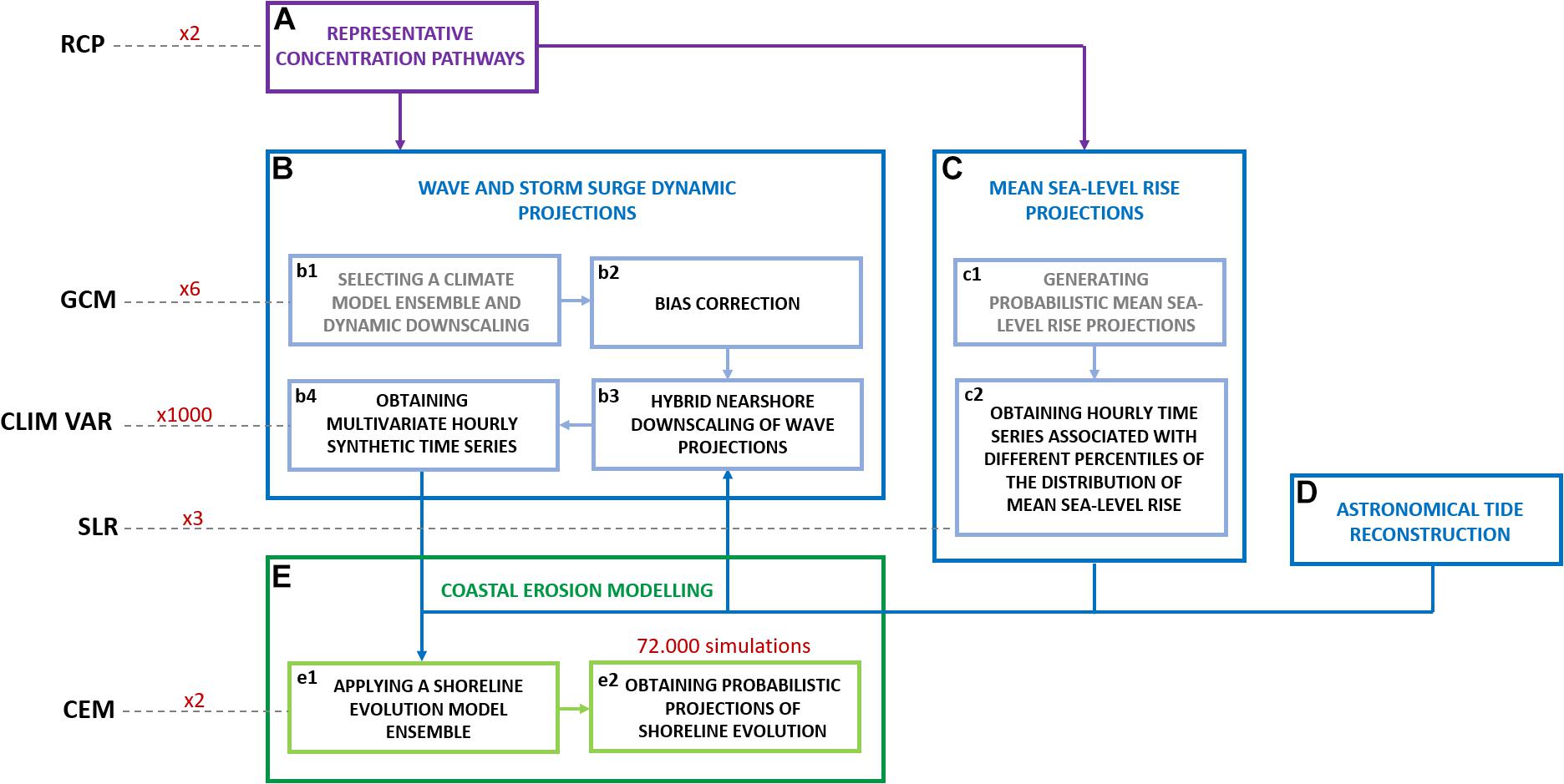
Figure 1. Flowchart describing the methodology proposed for the development of coastal erosion projections. Boxes A–E represent different components of the top-down approach and, in particular, boxes A (RCP ensemble), b2 (GCM ensemble), b5 (internal climate variability sampling denoted as CLIM VAR), c2 (SLR percentiles), and e1 (CEM ensemble) relate to the different levels of the cascade of uncertainty. Actions displayed in grey colour involve actions not undertaken in this study although used as input for other steps.

Projections of Mean Sea-Level Rise

Projections of global mean SLR provide insufficient information to support climate change adaptation, as local decisions require local projections that accommodate different risk tolerances (Kopp et al., 2014). In this study, we use complete probability distributions of regional mean SLR considering Antarctic ice-sheet (AIS) simulations (DeConto and Pollard, 2016), including ice-shelf hydrofracturing and ice-cliff collapse (DP16, Kopp et al., 2017). The use of explicit physics has led to a significant upward shift in central projections for the RCP4.5 and RCP8.5 scenarios with respect to its predecessor Kopp et al. (2014), which relies on expert assessment and elicitation. While DP16 projections are only based on a single AIS model and need further development to increase confidence (Hinkel et al., 2019), they allow expanding the space of the physically coherent and can be a useful tool to explore the uncertainty in future extreme outcomes.

We obtain probabilistic SLR projections at Gijon tide-gauge, using the code provided by Kopp et al. (2017), for the RCP4.5 and RCP8.5 scenarios. For both RCPs, we account for SLR uncertainty by considering the 5, 50, and 95th percentiles of the simulated frequency distributions. As can be observed in Figure 2, the projected 50th percentile increases from 0.59 to 0.90 m, and from 0.87 to 1.46 m from 2081 to 2100 under the RCP4.5 and the RCP8.5, respectively. While assuming constant acceleration of ice loss leads to an increase in forcing sensitivity, the central 90% of simulations by 2100 for the RCP4.5 (0.36–1.63 m) and the RCP8.5 (0.76–2.55 m), respectively, overlap near the mid-low RCP8.5 percentiles. The highest RCP8.5 percentiles spread significantly from the mean values.

FIGURE 2

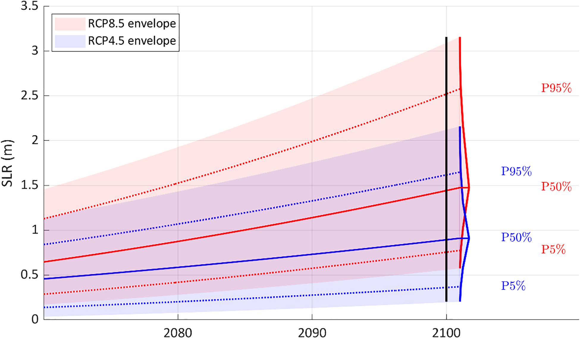
Figure 2. Probabilistic projections of local-mean sea-level rise at Gijon tide-gauge for RCP4.5 and RCP8.5 from 2070 to 2100 using Kopp et al. (2017) framework. Solid lines indicate 50th percentile; dashed lines indicate 5 and 95th percentiles; shaded areas represent the 0.5 and 99.5th percentiles of the SLR distribution for 2100.

Projections of Waves and Storm Surges

IHCantabria (2020) has recently generated dynamic multi-model projections of wave conditions and storm surge. Wave projections were developed for the Northeast Atlantic Ocean using the WaveWatch III third generation wave model (Tolman and The WaveWatch III^® Development Group, 2014). In the model, three regional grids (Artic, Atlantic and Spain-Atlantic with resolutions of 1° × 1°, 0.5° × 0.5°, and 0.1°×0.1°, respectively) were nested to a global grid with a resolution of 1°×1°. The global grid was forced with winds and ice coverage from 6 GCMs.

Storm surge projections were produced for the Atlantic and Mediterranean coast of Spain using the ROMS ocean circulation model (Shchepetkin and McWilliams, 2005) with a 0.08° × 0.06° resolution grid. The grid was forced with winds and sea level pressure from 6 GCMs.

Ensemble of Climate Models and Dynamic Downscaling

The wave and ocean models were forced with the outputs of the GCMs described in Supplementary Table 1. The selection of the GCMs (with spatial resolution between 0.75° and 2.5°) was based on the provision of the variables of interest at the required temporal resolution (3-hourly), time periods (1985–2005, 2026–2045, and 2081–2100) and concentration scenarios (RCP4.5 and RCP8.5), and on if these variables were derived from the same GCM realisation and initialisation. For this study, we consider the model simulations for both RCPs, 6 GCMs (ACCESS1.0, CMCC-CC, CNRM-CM5, HadGEM2-ES, IPSL-CM5A-MR, and MIROC5) from the Coupled Model Intercomparison Project 5 (CMIP5), and two time periods, the long-term future (2081–2100) and the historical reference (1985–2005).

The wave model was run following a multigrid configuration as for the development of the global ocean wave database GOW2 (Pérez et al., 2017). Earth2014 (Hirt and Rexer, 2015) and GSHHG (Global Self-consistent Hierarchical High-resolution Geography) databases were used to define the bathymetry and the coastlines, respectively. The bathymetric information for ROMS came from the EMODnet database. The GCM variables used to force the wave and ocean models were wind fields at 10 m over the sea surface level and concentrations of ice coverage (from 0 to 1), and surface wind fields and sea level pressure, respectively. GCM-derived variables were in both cases interpolated at each node of the computational grid at an hourly scale for the complete simulated periods.

Bias Correction

GCM outputs contain important biases when compared to observations, which need to be corrected before using them for impact studies. As these outputs are not synchronised with reanalysis or hindcast data, bias correction cannot be applied on an hourly basis but on the distributions or statistics of the variables to be corrected (Maraun, 2016). In recent years, different methods for bias correction have been developed. These range from simple techniques based on the delta method (Hay et al., 2000) that are convenient for monthly or annual data, to more sophisticated approaches based on quantile–quantile mapping that are more suitable when working at daily scales (Gutiérrez et al., 2018).

In this study, we apply the empirical quantile mapping (EQM) method. The EQM consists of analysing the distribution of observed values and adjusting some characteristics of the empirical probability distribution function with projected values by means of identifying quantiles. This adjustment applies to the wave and storm surge projections in the historical period (1986–2005) and in the future period (2081–2100) to correct the simulations (Dequé, 2007). The EQM is given by the following equation:

$$z={\text{CDF}}_{\text{obs}}^{-1}\left({\text{CDF}}_{\text{mod}}\left(y\right)\right)(1)$$

where z and y are the corrected and original values of the model, respectively; and CDF_obs and CDF_mod are the empirical cumulative distribution functions of the observations and the model, respectively.

We define the quantiles following linear spacing (q_i = 1, 5, 10,…, 90) and Gumbel distribution fitting (for quantiles over the 90th percentile). For each quantile, we obtain the correction term and interpolate linearly between them. Then, we extrapolate the data outside the predefined quantile range using the same correction term found for the first and last quantiles (Lemos et al., 2020). Additionally, we define bias as a time-invariant component of a model error. For the historical period (reference), we use the GOW2 database to correct the wave climate simulations (significant wave height, Hs, and peak period, Tp) and the GOS dataset (Cid et al., 2014) to correct the storm surge.

In order to validate the EQM-based bias correction, we compare the GOW2 and GOS distribution functions with the climatic data from the GCMs using the PDF_score (probability density function score), as proposed by Perkins et al. (2007). The PDF_score measures the degree of similarity of two probability density functions, allowing the comparison of entire time series without the limitation of having non-simultaneous climatic data over time (it takes value 1 when the functions are similar, and 0 when there is no overlap between them). Further details on the validation are provided in the Supplementary Material.

Figure 3 shows the comparison of the distribution function of Hs for each GCM in the historical period (1985–2005) with the GOW2 historical distribution. The CMCC model, which is the GCM with the highest spatial resolution, is the ensemble member that better reproduces the hindcast simulations. The other members of the GCM ensemble underestimate Hs. Figure 3A illustrates the distribution function of Hs at deep water from the GOW2 hindcast and the climatic data from the ensemble members (ACCESS1.0, CMCC-CC, CNRM-CM5, HadGEM2-ES, IPSL-CM5A-MR, and MIROC5) with the corresponding PDF_score. Figure 3B shows the Q–Q plot of the original (uncorrected) Hs per ensemble member against GOW2 Hs. Five ensemble members show a consistent underestimation, especially at the upper quantiles (i.e., extreme values, over the 99th percentile). Figures 3C,D display the distribution function and the Q–Q plot for the corrected Hs, showing how bias correction leads to a better agreement between each ensemble member and GOW2. The improvement in representing the most extreme events is due to the Gumbel distribution fitting for quantiles over the 90th percentile. Supplementary Figure 1 presents the equivalent analysis for the storm surge.

FIGURE 3

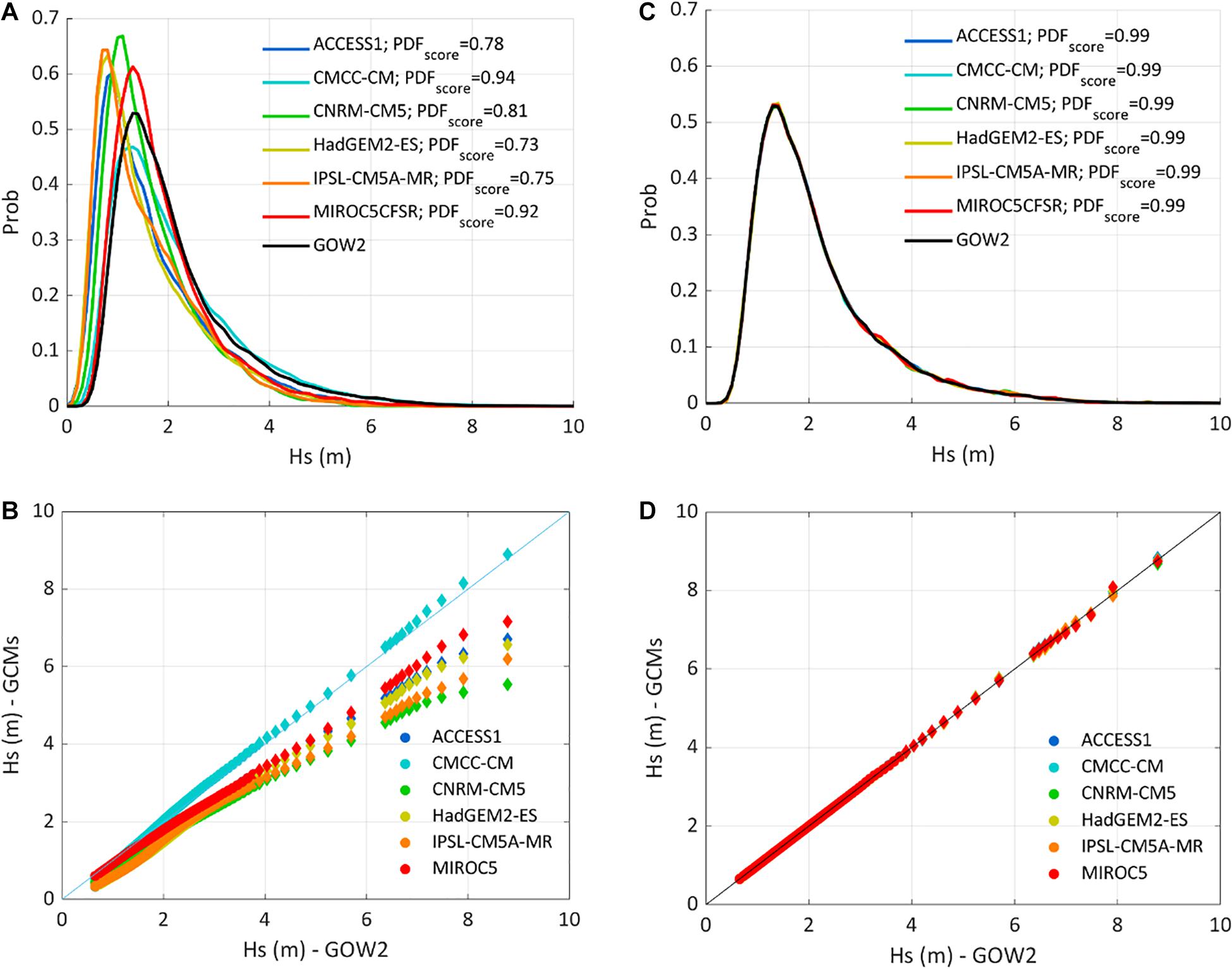
Figure 3. (A) Probability distribution function of Hs at deep waters from the hindcast GOW2 database and the uncorrected climatic data from each ensemble member (i.e., ACCESS1.0, CMCC-CC, CNRM-CM5, HadGEM2-ES, IPSL-CM5A-MR, and MIROC5) with the corresponding PDFscore. (B) Q–Q plot of the original uncorrected Hs, per ensemble member. (C) Probability distribution functions of GOW2 Hs and corrected Hs associated with each ensemble member. (D) Q–Q plot of the original uncorrected Hs, per ensemble member.

Hybrid Downscaling of Waves Projections

Despite the dynamic projections present very high resolution along the Spanish coast, we nest a coastal wave propagation model to capture wave transformations that result from interactions with the bathymetry and future sea level (SLR, projected storm surge and astronomical tides). Since downscaling hourly wave conditions for 2 RCPs and 6 GCMs considering 3 SLR trajectories requires a huge computational effort, hybrid downscaling techniques can offer advantage. We apply the hybrid downscaling technique developed by Camus et al. (2011), which combines mathematical tools (i.e., a selection algorithm and a multidimensional interpolation method) with numerical simulations to obtain the future wave forcings of the CEMs. The steps of the hybrid downscaling approach are: (1) selection of the closest node to the study beach from dynamical wave projections at 0.1° resolution along the Spanish coast and the closest wind node from the corresponding GCM, and collection of the time series of the state parameters Hs, Tp and mean direction, as well as the wind velocity and direction for the target time period (2081–2100) and from the 6 GCMs; (2) selection of a limited number of cases (500), which are the most representative of all possible future wave conditions at 0.1° resolution; (3) propagation of the selected cases using a wave transformation model for each scenario considered at four sea levels (0.0, 2.5, 5.0, and 8.0 m) that cover the whole casuistry of storm surge, tide, and SLR by the end of the century; and (4) reconstruction of the time series of sea state parameters near the beach (but outside the active sediment transport extent) for each RCP and SLR scenario, and for each GCM independently at the corresponding hourly sea level. These steps are illustrated in Supplementary Figure 2.

In order to select the subset of sea states that best represent wave conditions at 0.1° and wind, we apply the maximum dissimilarity algorithm (MDA). We use this subset of conditions as boundary conditions to the SWAN model (Booij et al., 1999) nesting three grids to achieve a spatial resolution of 20 m in the area of San Lorenzo Beach. During the simulations, wave amplification due to non-linear interactions between waves and projected sea level is accounted for as in Camus et al. (2019). For the reconstruction of the nearshore wave time series, we use a multidimensional interpolation method based on radial basis functions (RBF). RBFs allow to define a statistical relationship between the offshore wave parameters and nearshore conditions, which are the output of the SWAN model.

Generation of Multivariate Synthetic Time Series

In nature, wave conditions and storm surges are random. This means that while each GCM simulation is a precise rendering of the future climate, no GCM projection will happen (Mankin et al., 2020). Internal climate variability is an intrinsic uncertainty inherent to the climate problem (Giorgi, 2010), which could be addressed through using ensembles of transient and credible simulations starting at different times in the control period (Toimil et al., 2020a), also known as initial condition ensembles (Mankin et al., 2020). Here, we build upon already elaborated multi-model projections that may undersample internal climate variability uncertainty. For this uncertainty to be accounted for, we apply a vector autoregressive (VAR) model (Solari and van Gelder, 2012) that considers empirical functions to stochastically generate 1,000 multivariate hourly time series of waves and storm surges for each (RCP-)GCM over the time periods 1986–2005 and 2081–2100. Similar to an initial condition ensemble, this allows to produce a distribution of outcomes consistent with the same assumptions underlying the original GCM-driven runs.

Vector autoregressive models are extensions of autoregressive models for multivariate data. Autoregressive models provide the present value of an observation as a linear function of past observations. A similar VAR model based on GEV functions was applied in Toimil et al. (2017) to obtain multivariate hourly time series of waves and storm surges in San Lorenzo Beach using historical data.

The statistical analysis of the persistence regimes allows to verify that the VAR model is able to reproduce the temporal dependence structure of the original time series. Supplementary Figure 3 shows the persistence regimes of Hs over different thresholds and the joint probability distribution of sea state parameters and storm surge. The persistence regimes can be especially relevant when it comes to apply equilibrium models to reproduce the shoreline response to cross-shore forcing since their nature is such that a larger portion of the potential erosion (or accretion) can be attained for conditions which remain over long periods (Miller and Dean, 2004).

Coastal Erosion Modelling

The last step in the top-down approach is the coastal erosion modelling. CEMs can be sensitive to multiple factors, highly dependent on empirical parameters and present limitations to simulate physical processes realistically (Montaño et al., 2020; Toimil et al., 2020b). For this reason, we consider epistemic uncertainty in erosion modelling by performing an ensemble of CEMs. We set-up and apply two equilibrium models that couple short-term coastal dynamics and long-term SLR. The two models have been calibrated in the study beach over the period 1979–2020 using nearshore waves downscaled from GOW2, updated storm surges from GOS, and the reconstruction of the astronomical tide as forcing conditions, as well as aerial photographs and survey data as described in Toimil et al. (2017).

We run each CEM with 36,000 combinations of the projected forcing variables for the period 2081–2100 that result from 2 RCPs, 6 GCMs, and 1,000 synthetic multivariate hourly time series of waves and storm surges for each GCM and 3 alternative hourly SLR trajectories related to three percentiles. Additionally, we perform 6,000 extra runs with the forcing variables driven by the 6 GCMs over the period 1985–2005.

Ensemble of Cross-Shore Erosion Models

The CEMs we implement rely on the classical equilibrium or linear relaxation in which the difference with respect to an equilibrium term drives shoreline evolution (Eq. 2). This short-term shoreline response, which can be induced by time-varying water levels or breaking waves combines with a long-term response due to SLR in a coupled fashion.

$$\frac{dy(t)}{dt}=VG\Delta D(t)(2)$$

where y(t) is the shoreline position at time t; V is a constant governing the rate at which the shoreline approaches the equilibrium; G is a modulating function; and ΔD(t) is the disequilibrium term that forces shoreline evolution.

The first CEM we implement (CEM1) is the shoreline evolution model proposed by Toimil et al. (2017), which is composed of the equilibrium shoreline evolution model of Miller and Dean (2004) and a SLR-induced shoreline recession model that seeks to reproduce the landward displacement of the coast due to SLR, also known as the Bruun effect (Bruun, 1962). In this case, the shoreline change rate can adopt two values, one for erosion V = k⁻ and another one for accretion V = k⁺. The modulating function G is equal to one and the disequilibrium term responds to ΔD(t) = y_eq(t)−y(t). The equilibrium shoreline position thus combines short- and long-term effects following:

$$y_{eq}\left(t\right)=\mathrm{\Delta }{y}_0-W_b^{*}\left(t\right)\left(\frac{0.106H_b\left(t\right)+SS\left(t\right)+AT\left(t\right)}{B+2H_b\left(t\right)}\right)-W^{*}\left(t\right)\frac{SLR(t)}{B+h^{*}}(3)$$

where Δy₀ is an empirical parameter; $W_b^{*}$ is the active surf zone width determined from the break point by $W^{*}={\left(\raisebox{1ex}{$H_b$}\!\left/ \!\raisebox{-1ex}{$\gamma A$}\right.\right)}^{1.5}$, in which A is the profile scale parameter (Dean, 1991); H_b is the breaking Hs obtained using γ = 0.55 spectral breaking criteria; SS is the storm surge; AT is the astronomical tide; B is the berm height; W^∗ is the active beach profile width; and h^∗ is the depth of closure calculated using the empirical formula of Birkemeier (1985).

The second CEM we implement (CEM2) is an equilibrium energy-based model modified from Yates et al. (2009) to consider SLR effects. The shoreline change rate is approximated to be the same for erosion and accretion events V = C, the modulating function is V = E^1/2 (where E means the wave energy), and the disequilibrium term is ΔD(t) = E(t)−E_eq(t). The equilibrium energy term E_eq(t) accounts for the Bruun effect, which is treated as a long-term trend following Jaramillo et al. (2020):

$$E_{eq}\left(t\right)=a\left(y(t)+W^{*}\left(t\right)\frac{SLR\left(t\right)}{B+h^{*}}\right)+b(4)$$

CEM1 and CEM2 are forced with wave-breaking parameters, which we estimate from nearshore waves. Considering the large number of VAR-based realisations, we apply a simple propagation technique based on wave energy conservation, the Snell’s law of refraction, and a constant depth-breaking criterion.

Multi-Ensemble Probabilistic Projections of Shoreline Evolution

As a result of the thousands of CEM simulations, we obtain three different simulation packages (SP). The first SP (SP1) corresponds to 72,000 projected hourly shoreline evolutions from 2081 to 2100. These time series of shoreline change account for the uncertainty sampled at the steps of the top-down approach by considering 2 RCPs, 6 GCMs, 1,000 synthetic multivariate chronologies of future waves and storm surges for each RCP–GCM, 3 RCP–SLR trajectories related to three percentiles, and 2 CEMs. The second SP (SP2) includes 12,000 reference shoreline evolutions on hourly basis for the historical period 1985–2005, based on 6 GCMs, 1,000 synthetic multivariate chronologies of future waves and storm surges for each GCM, and 2 CEMs. Finally, the third SP (SP3) contains 72 projected hourly shoreline evolutions from 2081 to 2100 that differ from those of SP1 in that they do not consider climate variability uncertainty. The time series of shoreline change of SP3 account for 2 RCPs, 6 GCMs, 3 RCP–SLR trajectories related to three percentiles, and 2 CEMs.

Figure 4 displays the 72,000 simulations of SP1: 36,000 for the RCP4.5 (Figure 4A) and 36,000 for the RCP8.5 (Figure 4B). In each panel, shaded bands represent the 99% confidence levels related to the 5, 50, and 95th percentiles of SLR (colour code), superimposed by the simulations of SP3 (grey solid lines). The grey dashed line indicates the physical boundary of the beach (beyond this limit it would have disappeared). The blue and red dashed lines define the mean plus/minus standard deviation space associated with CEM1 and CEM2, respectively. As can be observed, such space is overall wider (higher upper-bound and lower lower-bound) for CEM2, especially resulting in larger erosion over time for the RCP–SLR combinations considered. Another aspect worth mentioning is the influence of GCMs internal climate variability in shoreline change. There is a hint that SP3 time series virtually never reach the 99% confidence levels of SP1, so not considering chronologies alternative to each GCM simulation could translate into the exclusion of potential outcomes. Importantly, these outcomes are more likely to be associated with erosion than with accretion phases, and this is more apparent for the RCP8.5. This may be because the exploration of different chronologies, even though they maintain the same pdf as the original GCM-driven simulations, may allow detecting different extreme retreat events that could result from cumulative effects such as less storm spacing or calm conditions over shorter periods of time.

FIGURE 4

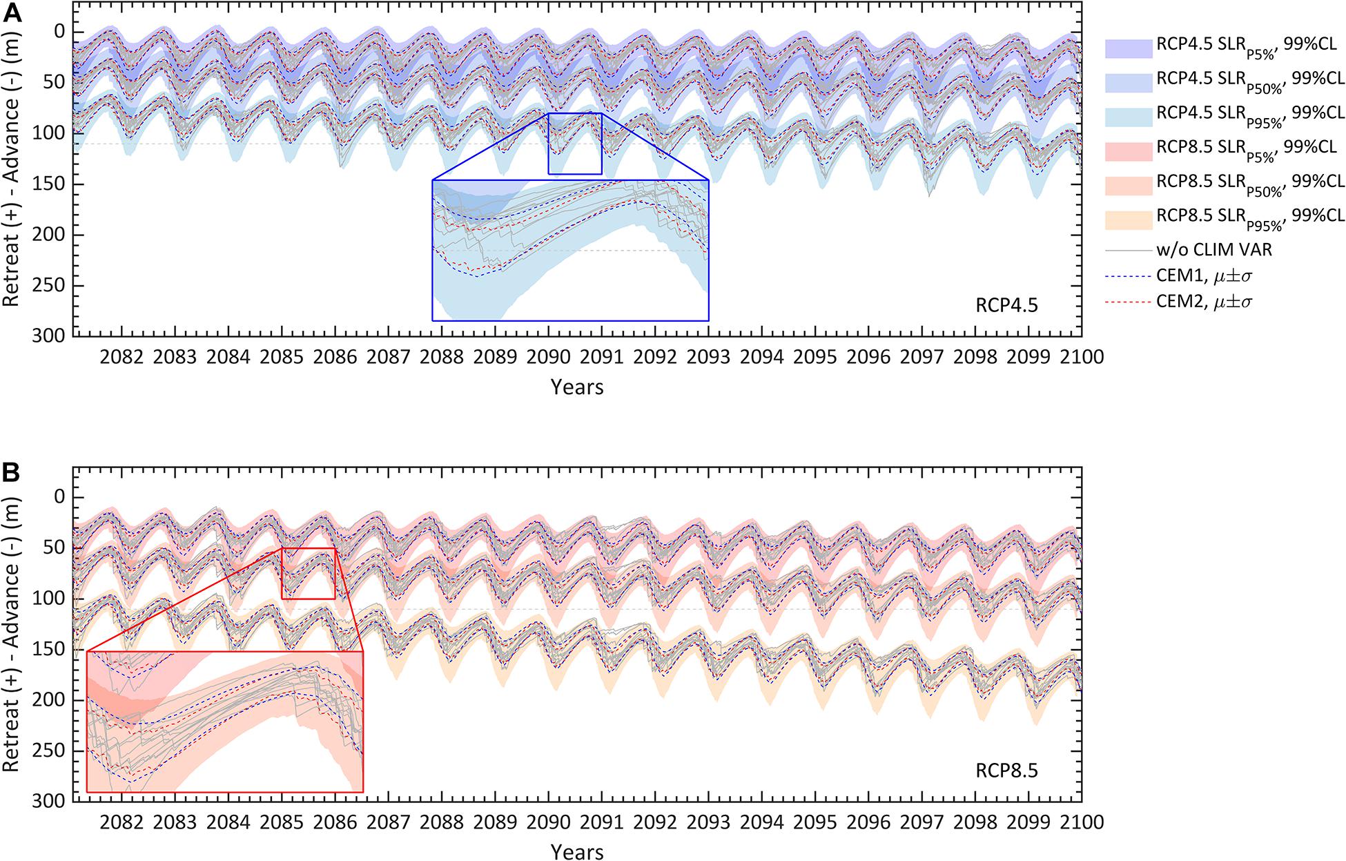
Figure 4. Shoreline evolution projections for the period 2081–2100 in San Lorenzo Beach. Shoreline position retreat (positive values) and advance (negative values) with respect to the present position. Coloured shaded bands and dashed lines are related to the 72,000 simulations of SP1 generated for 2 RCPs (RCP4.5 and RCP8.5, A,B, respectively), 6 GCMs (ACCESS1.0, CMCC-CC, CNRM-CM5, HadGEM2-ES, IPSL-CM5A-MR and MIROC5), 3 SLR percentiles (5, 50, and 95th), climate variability (1,000 multivariate realisations per each RCP-GCM) and 2 CEMs. The 72 simulations of SP3 (without considering climate variability) are represented by the grey solid lines. The grey dashed line represents the threshold beyond which the beach would have disappeared.

For both RCPs, results are strongly clustered by the SLR percentiles. In the case of the SLR 50th percentile, SP1 mean shoreline retreats increase from 52 to 64 m and from 75 to 103 m between 2081 and 2100 for the RCP4.5 and the RCP8.5, respectively. As expected, the greatest dispersion of the results occurs by 2100, where SP1 and SP3 shoreline retreats roughly range, respectively, between 9–138 and 25–115 m for the RCP4.5, and between 37–200 and 52–177 m for the RCP8.5. These ranges cover all possible outcomes from the lower bound of the 99% confidence level associated with the SLR 5th percentile to the upper bound of the 99% confidence level for the SLR 5th percentile.

Using the complete time series, we compute an indicator of the long-term or structural shoreline recession in 2081 and 2100 relative to 2005 (hereinafter R2081 and R2100, respectively) by subtracting the 2-year average initial position from the 2-year average final position of the shoreline from each model simulation. Additionally, we analyse changes in (episodic) extreme retreat events over the period 2081–2100 by fitting annual maxima shoreline retreats to non-stationary extreme value distributions. These outcomes are further described and analysed in section “Visualisation and Communication of Uncertainty in Coastal Erosion Projections”.

Visualisation and Communication of Uncertainty in Coastal Erosion Projections

Based on SP1, SP2, and SP3 shoreline evolution time series, we develop four analyses that provide different although complementary ways of visualising and communicating uncertainty in coastal erosion projections. We decompose the uncertainty cascade down to coastal erosion projections using real data, factorise long-term erosion estimates by the uncertainty dimensions deemed and determine their relative importance, and explore non-stationary extreme retreat events and the influence of climate variability on them.

The Cascade of Uncertainty

The paradigm of the cascade of uncertainty (Mitchell and Hulme, 1999; Wilby and Dessai, 2010) has been used in the literature to illustrate theoretically both the information and the uncertainty cascading across the modelling chain of the top-down approach, from the RCPs to coastal impact estimates, whether in the form of a triangle (e.g., Toimil et al.,2020a,b) or as a sequential diagram (e.g., Ranasinghe, 2016). However, more challenging is moving from theory to practice, particularly when the cascade extends down to impact models’ response. Figure 5 attempts to visualise the real cascade of uncertainty in coastal erosion projections in San Lorenzo Beach built upon actual data (SP1), expanding from the RCPs (upper tip where all lines converge; top layer) to the R2100 indicator (bottom layer). From top to bottom, the second layer shows an ensemble of 6 GCMs (ACCESS1.0, CMCC-CC, CNRM-CM5, HadGEM2-ES, IPSL-CM5A-MR, and MIROC5) forced by 2 future concentration pathways (RCP4.5 and RCP8.5). The following layer illustrates the role of uncertainty sampling in internal climate variability (denoted as CLIM VAR in the vertical axis). 1,000 multivariate realisations of potential chronologies of future wave conditions and surges for each RCP-GCM account for the stochastic nature of these dynamics. The fourth layer represents the combination of the multiple realisations of projected waves and storm surges with 3 different RCP-induced SLR trajectories (5, 50 and 95th percentiles) to force the CEMs. Next, each line splits into 2 CEMs, each of which delivers its corresponding R2100 value. For the sake of visibility and to avoid overplotting, we only plot 720 simulations (out of 72,000), although covering the full R2100 range, and distribute RCP, GCM, CLIM VAR, SLR, and CEM levels evenly in space, with R2100 reaching real values along the horizontal axis. Likewise, we neither depict the threshold beyond which the beach would have disappeared and that would be placed in 110 m (horizontal axis).

FIGURE 5

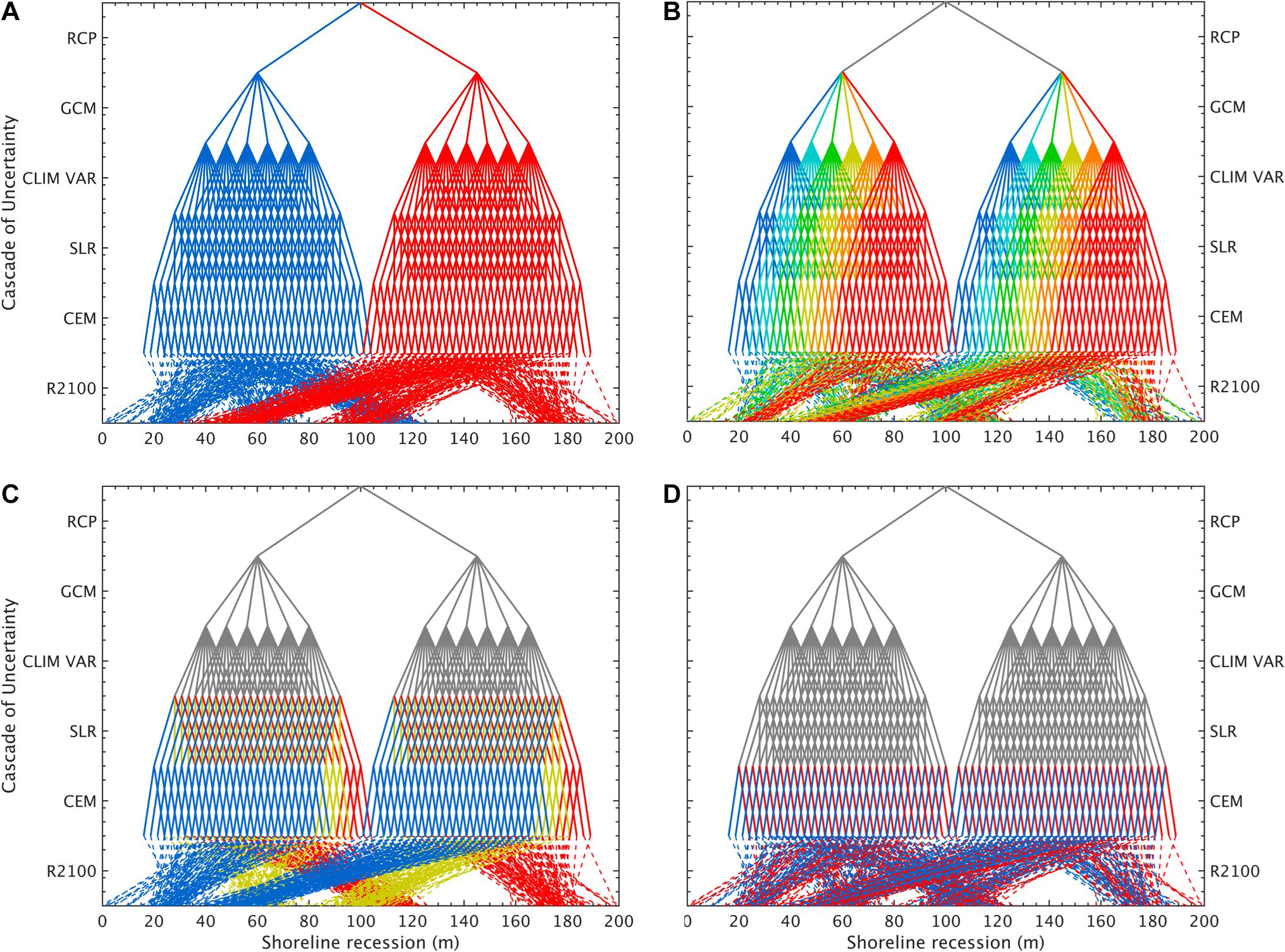
Figure 5. Visualisation of the cascade of uncertainty in coastal erosion projections by 2100. The cascade is built upon SP1 simulations. From top to bottom: first layer shows the 2 RCPs, second layer shows the ensemble of 6 GCMs, third layer shows climate variability, fourth layer shows the 3 SLR percentiles, fifth layer shows the ensemble of 2 CEMs and the last layer shows the R2100 indicator (actual values displayed on the horizontal axis). (A–D) illustrate the cascade under four factorisations that highlight the uncertainty spread due to the choice of RCPs, GCMs (considering climate variability realisations), SLR percentiles, and CEMs. For the sake of visibility, we plot 720 SP1 simulations (out of 72,000) covering the full range of 2100 and distribute RCP, GCM, CLIM VAR, SLR, and CEM levels evenly in space.

Figures 5A–D illustrate the cascade of uncertainty in R2100 under four different factorisations. These factorisations seek to disentangle the uncertainty in R2100 estimates based on the choice of RCP (Figure 5A), GCM including the associated climate variability realisations (Figure 5B), SLR percentile (Figure 5C), and CEM (Figure 5D). As such, the range of R2100 values is the same in all panels, extending roughly from 0 to 200 m. In Figure 5A, each colour shows a different RCP-driven R2100 pathway (RCP4.5-blue and RCP8.5-red). Thus, the ensemble of GCM forced by the same RCP are coloured alike, and the same applies to the subsequent layers down to coastal erosion projections. In Figure 5B, we start decomposing by GCM and each colour represents a different GCM-driven R2100 pathway (ACCESS1.0-blue, CMCC-CC-cyan, CNRM-CM5-green, HadGEM2-ES-yellow, IPSL-CM5A-MR-orange, and MIROC5-red). Likewise, in Figure 5C, SLR percentiles are decomposed next and coloured according to the R2100 pathway they drive (P5%-blue, P50%-yellow, and P95%-red). Finally, Figure 5D shows R2100 factorised by the CEM dimension (CEM1-blue and CEM2-red).

Looking at the bottom layer, the dashed lines thus inherit their colour from the choices of RCP, GCM, SLR percentile, and CEM and allow to visualise the uncertainty range in R2100 that can be attributed to them at a glance. For instance, R2100 roughly range from 0 to 120 m for the RCP4.5 and from 30 to 200 m for the RCP8.5 (Figure 5A). As we focus on the long term (2100), GHG concentration differences are high and the different scenarios clearly represent two different R2100 populations that cannot be easily merged, which is further emphasised by the choice of SLR percentile (colour differentiated in Figure 5C). This results in a strong multi-modal response in R2100 induced by RCP–SLR with 4 different clusters: (1) P5% RCP4.5–SLR, (2) P50% RCP4.5–SLR and P5% RCP8.5–SLR, (3) P95% RCP4.5–SLR and P50% RCP8.5–SLR, and (4) P95% RCP8.5–SLR. This could be explained by the facts that we concentrate in a far future and that DP16 projections provide SLR extreme outcomes (e.g., a rise of 2.55 m for the RCP8.5 by 2100 in Gijon). Such multi-modal response gets weaker as we move into close time horizons. Supplementary Figure 4 shows the equivalent cascade of uncertainty for R2081 (also calculated using SP3 data). As it illustrates, not only are the clusters more diffuse by 2081, but the uncertainty spread in coastal erosion projections has narrowed and shifted toward smaller values on the horizontal axis.

Figure 5D reinforces the idea that, in general, CEM2 (wave energy-based including SLR trend) provides more extreme values, widening the range and thus, the uncertainty, in R2100. The GCM dimension (Figure 5B) does not appear to dominate the spread in the simulated projections. However, that does not mean that the additional simulations derived stochastically do not play an important role. Figure 6 shows the same plots as in Figure 5 but with the superimposition of SP3 R2100 (72 simulations) represented by solid black lines, which cover shoreline retreats roughly ranging from 15 to 185 m. R2100 uncertainty spread is thus increased by nearly 20% when considering a more complete sampling of climate variability compared to the more common approach of using a single realisation of GCM-driven wave and storm surge projections. This could be because, while it is known that the chronology can highly influence short-term shoreline changes (Toimil et al., 2017), certain chronologies may eventually affect long-term erosion (R2100), which if disregarded may lead to the misallocation of adaptation resources.

FIGURE 6

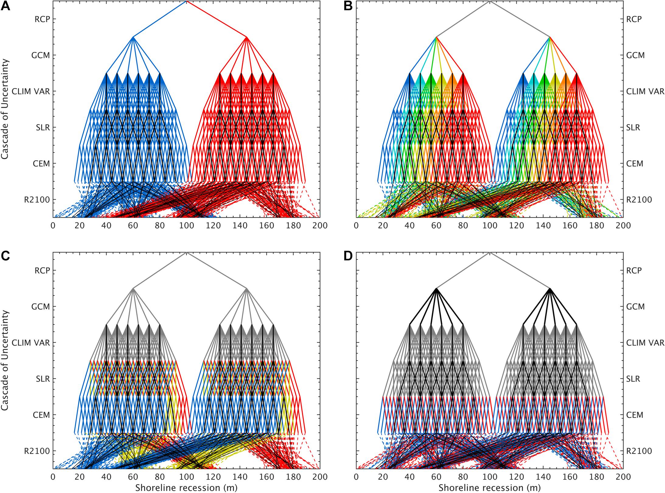
Figure 6. Visualisation of the cascade of uncertainty in coastal erosion projections by 2100 using SP1 and SP3 simulations. SP1 data (720 simulations out of 72,000) is displayed as in Figure 5 and SP3 data (72 simulations) are superimposed and represented by solid black lines. From top to bottom: first layer shows the 2 RCPs, second layer shows the ensemble of 6 GCMs, third layer shows climate variability, fourth layer shows the 3 SLR percentiles, fifth layer shows the ensemble of 2 CEMs and the last layer shows the R2100 indicator (actual values displayed on the horizontal axis). (A–D) illustrate the cascade under four factorisations that highlight the uncertainty spread due to the choice of RCPs, GCMs (considering climate variability realisations), SLR percentiles, and CEMs.

Factorisation of Uncertainty Sources

The R2100 cascade of uncertainty shows a clear multi-modal response dominated by the choice of the RCP and the SLR percentile. To isolate the effects of each uncertainty source over the coastal erosion projections, Figure 7 illustrates R2100 values factorised by the dimensions considered in absolute terms (column on the right) and nondimensionalised by SLR (column on the left). These R2100 values are based on SP1 (72,000 simulations accounting for climate variability) and SP3 (72 simulations not considering climate variability) data, which are represented using coloured and black symbology, respectively. R2100 values are factorised by their driving RCPs (Figures 7A,B), GCMs (Figures 7C,D) and CEMs (Figures 7E,F), all of which are in turn disaggregated by the SLR percentiles (5, 50, and 95th).

FIGURE 7

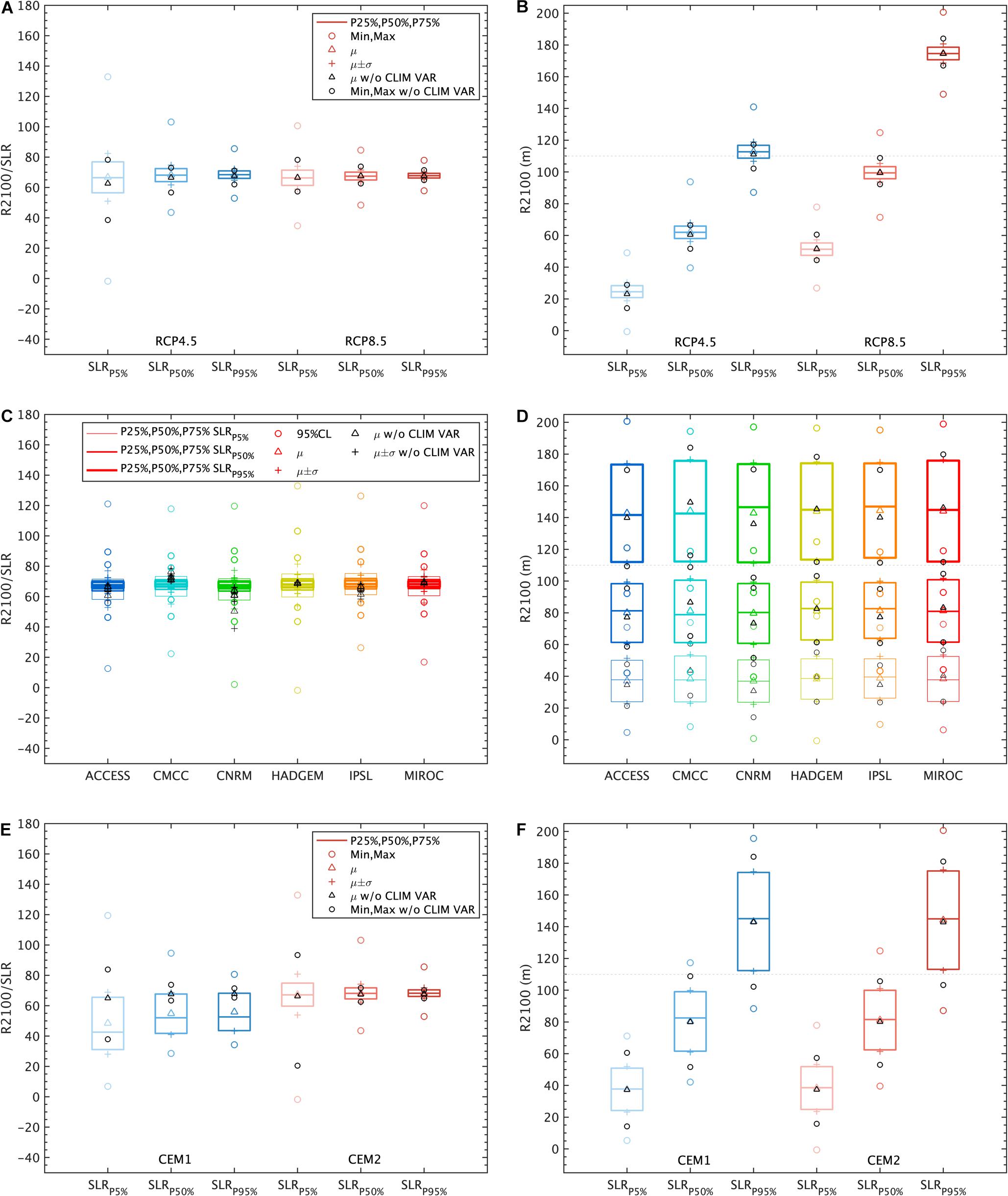
Figure 7. R2100 values factorised by their driving RCPs (A,B), GCMs (C,D) and CEMs (E,F), all of them disaggregated in turn by the SLR percentiles (5, 50, and 95th). R2100 factorisation is provided in absolute terms (m) on the right column and nondimensionalised by SLR on the left column. SP1 (72,000 simulations considering climate variability) and SP3 (72 simulations without considering climate variability) are represented using coloured and black symbology, respectively. Note that in B,D and F the grey dashed line represents the threshold beyond which the beach would have disappeared.

One of the most apparent features of Figure 7 is the role of climate variability in the R2100 spread range. While SP3 mean values can be either above or below SP1 mean values, SP3 maximum and minimum values are far (or very far in nondimensionalised panels) from the same statistics of SP1, highlighting the fact that not quantifying internal variability’s full extent sufficiently could be critical from a decision standpoint. As can be observed in Figure 7D, the variability inter-GCM for any SLR percentile is low for SP3 data, and very low for SP1. This could be expected because the multi-model projections of waves and storm surges show very little change in the signal and among GCMs, and due to the fact that we have corrected their bias (this can be deemed some sort of standardisation) and generated thousands of realisations with the VAR model under the same assumptions.

The highest the SLR percentile, the most the R2100 spread range is reduced when nondimensionalised, a reduction that is more significant for the RCP8.5 (Figure 7A) and longer-term horizons (Supplementary Figure 5). This could be explained because the higher the SLR, the more it dominates the central values of the R2100 distribution and, although the variability range is similar regarding the SLR percentile in absolute terms, when nondimensionalised by SLR, this variability is reduced the higher the SLR value. This decrease is sharper for the 25–75th percentiles of CEM2-driven R2100 than for CEM1-related outcomes (Figure 7E). However, CEM2 minimum and maximum values are shown to be more extreme than those from CEM1, whether or not nondimensionalised, as partly seen in Figures 5, 6.

Fraction of the Total Uncertainty

To further quantify the dominant drivers of uncertainty in these projections of coastal erosion and their relative contribution to R2100 uncertainty, we apply a four-factor, ANOVA-based variance decomposition to three experiments where RCPs, GCMs, SLR percentiles and CEMs are the uncertainty sources. The first experiment (A) consists of comparing the variance partitioning between SP1 72,000 simulations and SP3 72 simulations (A1 and A2, respectively). The second experiment (B) compares this variance partitioning between SP1 and SP3, both excluding the SLR 95th percentile (48,000 and 48 simulations, and B1 and B2, respectively). Finally, the third experiment (C) concentrates on the RCP8.5 and the SLR 50th percentile of SP1 and SP3, which reduces the simulations involved to 12,000 and 12 (C1 and C2), respectively.

Figure 8 shows for the experiments A–C the contribution of the uncertainty sources and their interaction to R2100 total uncertainty. The findings are consistent with the results obtained from previous analyses. Overall, we find a strong dominating influence of the SLR and RCP dimensions, which could be attributable to the horizon considered (2100), where RCPs diverge significantly, and the extreme SLR projections used.

FIGURE 8

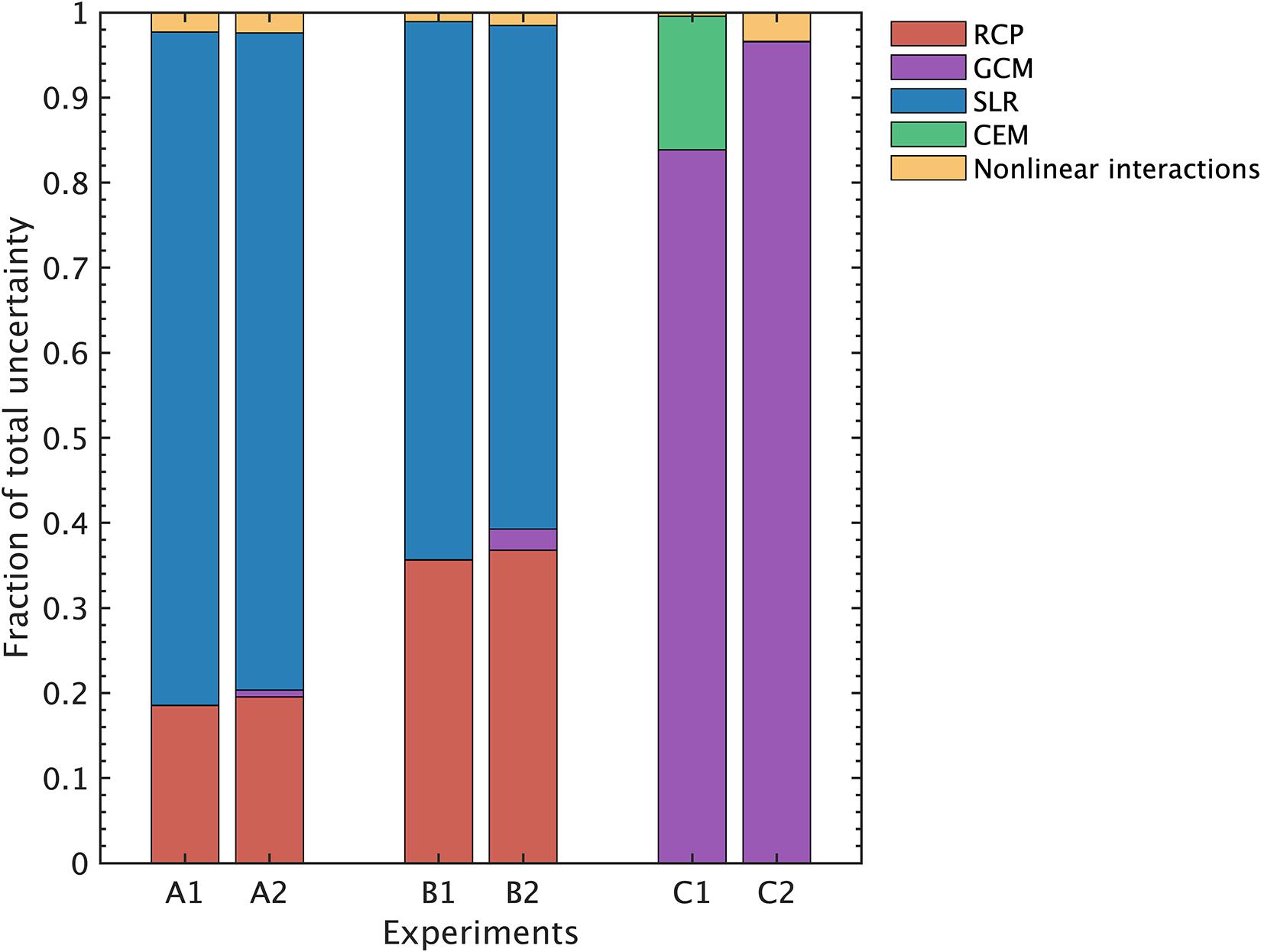
Figure 8. Contribution of each uncertainty source (RCPs, GCMs, SLR percentiles, and CEMs) and their interactions to total R2100 uncertainty. The variance partitioning is based on a four-factor ANOVA-based decomposition method. Experiment A compares SP1 72,000 simulations, with SP3 72 simulations (A1 and A2, respectively); experiment B compares SP1 48,000 simulations and SP3 48 simulations, both excluding the SLR 95th percentile (B1 and B2, respectively); and experiment C compares SP1 12,000 simulations and SP3 12 simulations, both constrained to RCP8.5 and SLR 95th percentile (C1 and C2, respectively).

Experiment A highlights the virtually negligible influence of GCM uncertainty (∼0%) compared with RCP’s (∼18%) and SLR’s (>80%) when considering the full range of R2100 (SP1, A1). This could be explained by the fact that the 1,000 additional realisations per each RCP–GCM to sample intrinsic uncertainty hide the variability of the GCMs themselves (Figure 7D), to which bias correction has also been applied. In A2, while SLR (∼75%) and RCP (∼20%) uncertainty continue to dominate, there is some (although little) room for GCM uncertainty contribution (∼1%).

As DP16 projections provide extreme SLR outcomes, experiment B seeks to analyse how the contributions would change if the SLR upper bound were the 50th percentile. Compared to experiment A, RCPs’ uncertainty contribution increases (∼36 and ∼37% for B1 and B2, respectively), SLR’s decreases (∼64 and ∼60% for B1 and B2, respectively) and, as could be expected, GCMs’ increases its relative importance (up to 3%) as for B2.

Finally, experiment C leaves RCP and SLR out of the equation. As a result, GCM uncertainty dominates but its contribution is still weaker in C1 than in C2 (∼84 and ∼97%, respectively) because of the effect of climate variability uncertainty. In C1 there is new room for the contribution of CEM uncertainty (∼16%). In any case, the contribution of the pairwise (RCP–GCM, RCP–SLR, RCP–CEM, GCM–SLR, GCM–CEM, and SLR–CEM) triple (RCP–GCM–SLR, RCP–GCM–CEM, RCP–SLR–CEM, and GCM-SLR-CEM) and quadruple (RCP–GCM–SLR–CEM) interactions to R2100 uncertainty is <3%.

Non-stationary Extreme Value Analysis and Influence of Climate Variability

Extreme shoreline positions are characterised by return levels of erosion, which can provide very valuable information for decision-making, as risk-reduction actions (e.g., beach nourishment design) often take place in response to unusually large shoreline recession. The analysis of the variability of extreme erosion events, however, is a complex issue as processes at two different time scales occur simultaneously: the interannual variability due to the combined effect of waves and storm surges, and the slow-onset SLR and its long-term effect, which leads to the gradual, persistent landward and upward displacement of the coastline. SLR, thus, introduces a positive and persistent erosive trend that can only be properly addressed by conducting non-stationary extreme-value analysis.

In this study, we use the Non-stationary Extreme Value Analysis (NEVA) package (Cheng et al., 2014) to estimate effective return levels, which indicate the return level that should be considered to have the same probability of occurrence over time. In NEVA, non-stationarity is based on the assumption that the location parameter of the Generalised Extreme Value (GEV) distribution is linearly time dependent according to the trend. We apply the non-stationary GEV distribution to annual maxima shoreline retreats. We obtain the effective return levels corresponding to 10, 25, and 50 years over the period 2081–2100 for the SP1 and SP3 time series of shoreline evolution. Figure 9 illustrates the time evolution of mean effective return levels (SP3, grey solid lines) and 99% confidence levels (SP1, coloured shaded areas) disaggregated by SLR percentiles and RCPs, where only time series with significant SLR trend are shown. There is more overlap among the RCP4.5 results (upper panels), especially for the SLR 50 and 95th percentiles and longer return levels. For the RCP8.5 (red panels), the mean effective return level of a 10-year extreme erosion in 2080 is 58.9, 92.8, and 140.7 m, while in 2100 is 78.8, 127.1, and 202.6 m for the 3 SLR percentiles, respectively. As can be observed, the time evolution of the effective return levels for the 6 GCMs of SP3 simulations has significant variability, which increases considerably for SP1 outcomes (with VAR-based simulations). The 99% confidence bands become wider as the corresponding year of the return level gets higher. These bands are asymmetric, with the higher spread of the return levels with respect to the mean for the high percentiles rather than for the low ones. Overall, RCP4.5’s exhibit higher variability and this could be explained by the lesser influence of SLR, which leads to chronology having greater impact on the results.

FIGURE 9

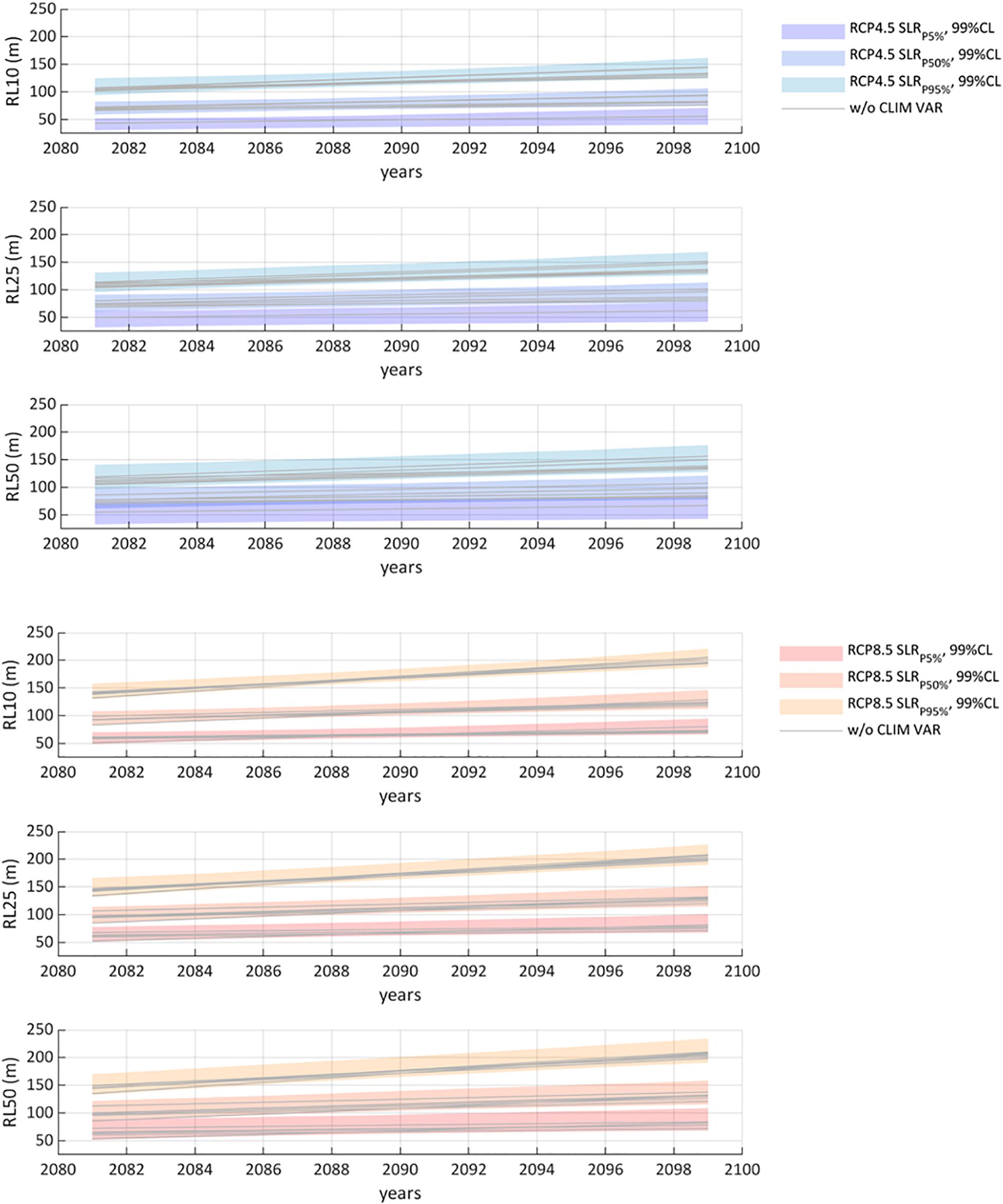
Figure 9. Effective return levels corresponding to 10, 25, and 50 years under the non-stationary assumption for the period 2080–2100 and for the SLR trajectories (associated with the 5, 50, and 95th percentiles) under the RCP4.5 (blue panels) and the RCP8.5 (red panels). Grey solid lines represent the return periods calculated from the GCM-driven simulations of SP3 (without climate variability). Coloured shaded areas show the 99% confidence bands of the non-stationary GEV fit to the annual maxima shoreline retreats derived from SP1 simulations.

Figure 10 shows the time series of annual maxima shoreline retreat for the IPSL-CM5A-MR model (solid grey line), where we compare its original run (SP3) and four different VAR-based simulations (#74, #294, #314, and #345 of SP1, represented by solid black lines) for the RCP8.5. We calculate the shoreline retreat annual maxima trend for each simulation (dashed lines). The trends of the SP3 run and the simulation #74 are similar (Figure 10A). However, the trends of the other three VAR-based simulations (Figures 10B–D) are higher than the SP3 run due to more erosive shoreline retreat evolution over the period 2081–2100. These higher trends reflect a higher increase of effective return levels of 25 years by 2100 compared to those from the SP3 run (pink lines). In addition, we find that shoreline retreat in 2081 influences the effective return levels over the following years. Take the case of simulation #314 (Figure 10C), where shoreline retreat is significantly lower than for the SP3 run, constraining the return level reached in 2100, although with a higher trend. The return level of the simulation #294 (Figure 10B) reflects by 2100 a combination of large shoreline recession in 2081 and a high erosion trend. The interannual variability of this return levels thus explains the wide extension of the confidence bands of the effective return levels, especially as for the upper bound. This confirms the influence of sampling climate variability uncertainty using the VAR model in the R2100 indicator identified in the previous analysis.

FIGURE 10

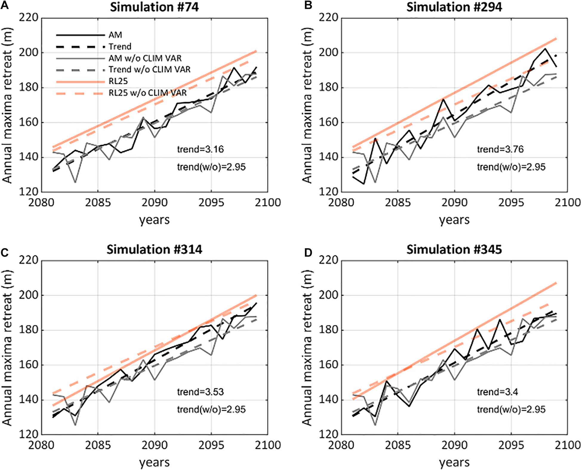
Figure 10. Time series of annual maxima shoreline retreat corresponding to the IPSL-CM5A-MR model (solid grey line) and the simulations #74 (A), #294 (B), #314 (C), and #345 (D) of SP1 associated with this GCM (solid black line). Dashed lines represent the annual maxima shoreline retreat trends. Effective 25-year return levels under the non-stationary assumption over 2080–2100 for the SLR 95th percentile and for the RCP8.5. The pink solid line shows the results of the SP1 simulation; and the pink dashed line represents the results associated with the original GCM simulation (SP3).

It seems that the chronology of the sea state parameters and storm surge is the factor that most influences the interannual evolution of shoreline retreat, rather than the magnitude of these dynamics during storms. To further verify the effect of climate variability in short-term erosion, we analyse the relationship between the number of storms per year and the annual maxima shoreline retreat over the historical period of several IPSL-CM5A-MR simulations of SP2 (Figure 11). We define storm events as independent 3-day events over the threshold of Hs that guarantees an average of 3 storms per year. For instance, the largest shoreline retreat in simulation #74 (Figure 11A) exceeds 42 m and happens in 1993 due to the cumulative effect of more than 10 storms over that year. Another example is the maximum shoreline retreat in simulation #294 (Figure 11B, higher in magnitude than in #74), which roughly reaches 52 m in 1999 because of the combined effect of many storms and a positive erosive trend over the previous years. In simulations #314 and #345 (Figures 11C,D, respectively), the largest annual maxima shoreline retreat occurs due to the significant erosion over the two preceding years (the beach is not able to recover in summer) induced by the large number of storms per year. In the original IPS-CM5A-MR run, the maximum shoreline retreat does not exceed 37 m and occurs in 1994, when also the highest number of storms happened (Supplementary Figure 6). From this analysis, we can conclude that the most extreme shoreline retreats are generated by “extreme” synthetic chronologies of wave and storm surge conditions simulated by the VAR model.

FIGURE 11

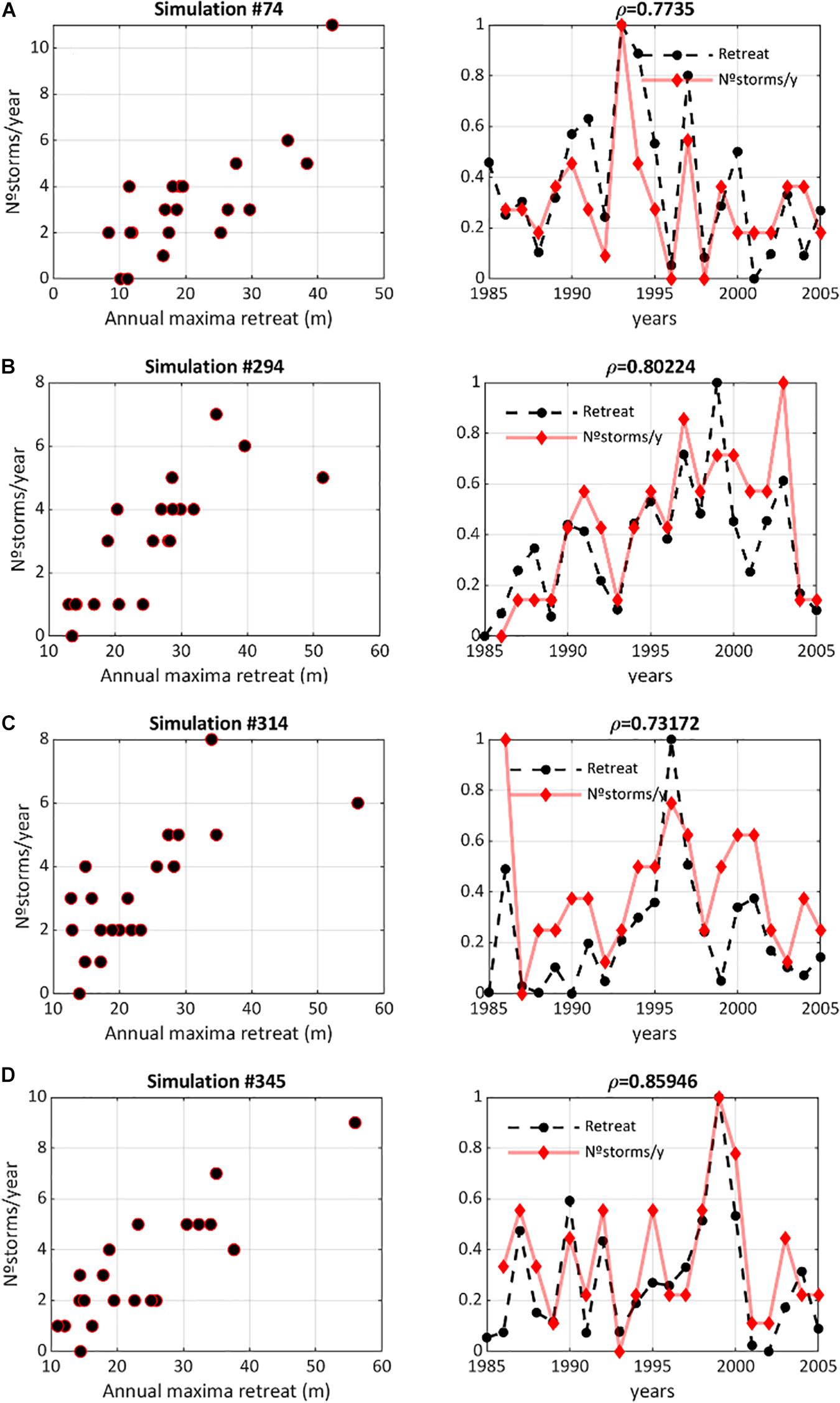
Figure 11. Scatter plot of the annual maxima shoreline retreat compared to the annual number of storms (left column). Time series of the normalised annual maxima shoreline retreat and normalised annual number of storms for the simulations #74 (A), #294 (B), #314 (C), and #345 (D) of SP2 associated with the IPSL-CM5A-MR model in the historical period (1985–2005) (right column).

Conclusion

Climate projections have brought into focus the imperative need to adapt coastal areas to a changing climate under conditions of deep uncertainty. Positioning decision-making in the best situation requires substantial efforts to better attribute uncertainty in impact assessments. This involves identifying and sampling sources of uncertainty and considering their nature, spreading and cumulative effect. The visualisation of this whole process can help understand the relative importance of the steps of the top-down approach to full uncertainty in impact estimates and where to concentrate energy and resources.

In this paper, we developed long-term multi-ensemble probabilistic coastal erosion projections following the steps of the top-down approach with the primary objectives of decomposing and visualising the cascade of uncertainty using real data and analysing the contribution of each step to the total uncertainty. For that purpose, we compiled dynamic projections of waves and storm surges (for 2 representative concentration pathways and 6 global climate models), corrected their bias and transferred projected offshore waves to nearshore by applying a hybrid downscaling technique that allows to consider sea-level effects on wave propagation. Next, we stochastically generated 1,000 additional multivariate realisations of projected waves and storm surges per each combination of representative concentration pathway and global climate model to account for different chronologies potentially driven by climate variability. We combined these 12,000 time series of future nearshore waves and storm surges with three mean sea-level rise trajectories corresponding to 3 percentiles of the simulated frequency distributions for the radiative forcing scenarios considered. Finally, we forced 2 coastal erosion models and derived 72,000 future time series of shoreline evolution. Based on these time series we calculated long-term and episodic (non-stationary) erosion, which could be useful tools to inform decision-makers on the shoreline future mean position and its variance.

It is noteworthy to mention that our choice to have applied bias correction before the hybrid downscaling in this study is based on the availability of reliable historical wave data in deep water. Besides, we consider that it is more realistic to propagate every hourly sea state at each corrected sea level, and this implies to correct the storm surge bias before downscaling waves. However, these two steps could be exchanged if robust historical nearshore data are available to apply the correction.

By means of this approach, we considered both knowledge uncertainty and intrinsic uncertainty. The first was characterised by using ensembles of representative concentration pathways, global climate models, and coastal erosion models, and a range of mean sea-level rise trajectories. Intrinsic uncertainty was accounted for by performing multiple multivariate realisations of projected waves and storm surges that were based on the same assumptions that the original projections but provided alternative chronologies that allowed to consider an overall larger range of variability and different extreme retreat events. Further developments of this approach could consider additional uncertainty sources such as coastal erosion model parameterisations (e.g., model coefficient adjustments would be needed as the 1979–2020 model structure will not necessarily remain unaltered in the future) or the application of different bias correction methods.

Two aspects that highly conditioned the results were our focus on the far future (2081–2100) and the use of projections of mean sea-level rise using Antarctic ice-sheet simulations. A justification for these choices is that risk assessments usually consider far-future lead times (i.e., 2100) and always require the full range of potential damaging outcomes, including low-probability high-impact scenarios. In the visualisation of the cascade of uncertainty, this resulted in a multi-modal response that was stronger in 2100 than in 2081, and where we identified four different clusters combining representative concentration pathways and mean sea-level rise percentiles. Both the cascade and the subsequent factorisation of long-term coastal erosion values highlighted that not quantifying internal variability’s full extent sufficiently could lead to a truncated range of outcomes, and adverse implications for decision-making. Another key feature relates to the influence of climate models uncertainty to the total uncertainty, which we found virtually negligible for the simulations that consider climate variability uncertainty sampling, partly due to the climate variables considered and bias correction (necessary for impact assessments), and because of the thousands of multivariate realisations we produced stochastically. Such realisations have the same underlying assumptions but provide alternative chronologies of wave conditions and storm surges. This noise itself has proven to be an important part of the full range of outcomes, as we found that the most extreme annual maxima shoreline retreats occurred for synthetic chronologies simulated by the stochastic model. These findings show that in order to capture the full uncertainty in coastal erosion projections, all uncertainty sources need to be adequately sampled considering case-specific aspects such as the climate variables, the degree of anthropogenic impact (e.g., radiative forcing or Antarctic ice-sheet contribution) and time horizon. In the near future (e.g., 2021–2050), the small differences in greenhouse gas concentration between radiative forcing scenarios could show greater inter-model variability, which would be similar to a random sample of realisations from the same climate model (e.g., as in Fernández et al., 2019). Further, projected changes in wave conditions and storm surge are relatively small in the study area. However, in other regions where future changes are more significant and the deviation in the ensemble projections is wider, climate model uncertainty could certainly account for a larger fraction of the total uncertainty.

Importantly, this study should be viewed as a way to expand scientific understanding of uncertainty treatment in coastal erosion projections when using the top-down approach, rather than providing the best projections of what coastal erosion in San Lorenzo Beach will be like. In particular, we tried to make progress on the incorporation, visualisation and analysis of the sources of uncertainty involved. For the sake of facilitating a better explanation of our final aim, namely visualising the uncertainty we used a pilot site for which data and models were at hand. The combination of better suited climate projections, improved downscaling methods and more detailed coastal erosion models (including more sophisticated wave-breaking propagation) would presumably result in a different range of shoreline recession values, and extreme retreat events of different magnitude and frequency. However, the approach and the uncertainty treatment herein proposed applies in any case.

Data Availability Statement

The original contributions presented in the study are included in the article/Supplementary Material, further inquiries can be directed to the corresponding author/s.

Author Contributions

AT developed the concept and wrote the original manuscript. AT and PC designed the analysis and designed the figures and their descriptions. AT, PC, and MA-C performed the analysis. IL verified the analysis. AT, PC, MA-C, and IL discussed and commented on the manuscript. All authors contributed to the article and approved the submitted version.

Funding

AT acknowledges the financial support from the FENIX Project by the Government of Cantabria. This research was also funded by the Spanish Government via the grant RISKCOADAPT (BIA2017-89401-R).

Conflict of Interest

The authors declare that the research was conducted in the absence of any commercial or financial relationships that could be construed as a potential conflict of interest.

Acknowledgments

The authors thank the Working Group on Coupled Modelling of the World Climate Research Programme, which is responsible for the CMIP, and the climate modelling groups for producing and making available their model output.

Supplementary Material

The Supplementary Material for this article can be found online at: https://www.frontiersin.org/articles/10.3389/fmars.2021.683535/full#supplementary-material

References

Athanasiou, P., van Dongeren, A., Giardiono, A., Vousdoukas, M. I., Ranasinghe, R., and Kwadijk, J. (2020). Uncertainties in projections of sandy beach erosion due to sea level rise: an analysis at the European scale. Sci. Rep. 10:11895.

Google Scholar

Birkemeier, W. A. (1985). Field data on seaward limit of profile change. J. Waterw. Port. Coast Ocean. Eng. 111, 598–602. doi: 10.1061/(asce)0733-950x(1985)111:3(598)

CrossRef Full Text | Google Scholar

Booij, N., Ris, R. C., and Holthuijsen, L. H. (1999). A third-generation wave model for coastal regions 1. Model description and validation. J. Geophys. Res. Oceans 104, 7649–7666. doi: 10.1029/98JC02622

CrossRef Full Text | Google Scholar

Bruun, P. (1962). Sea-level rise as a cause of shore erosion. J. Waterways Harbors Division ASCE 88, 117–130. doi: 10.1061/jwheau.0000252

PubMed Abstract | CrossRef Full Text | Google Scholar

Camus, P., Méndez, F. J., and Medina, R. (2011). A hybrid efficient method to downscale wave climate to Coastal areas. Coast. Eng. 58, 851–862. doi: 10.1016/j.coastaleng.2011.05.007

CrossRef Full Text | Google Scholar

Camus, P., Tomás, A., Díaz- Hernández, G., Rodríguez, B., Izaguirre, C., and Losada, I. J. (2019). Probabilistic assessment of port operation downtimes under climate change. Coast. Eng. 147, 12–24. doi: 10.1016/j.coastaleng.2019.01.007

CrossRef Full Text | Google Scholar

Cheng, L., AghaKouchak, A., Gilleland, E., and Katz, R. W. (2014). Non-stationary extreme value analysis in a changing climate. Clim. Change 127, 353–369. doi: 10.1007/s10584-014-1254-5

CrossRef Full Text | Google Scholar

Cid, A., Castanedo, S., Abascal, A. J., Menéndez, M., and Medina, R. (2014). A high resolution hindcast of the meteorological sea level component for Southern Europe: the GOS dataset. Clim. Dyn. 43, 2167–2184. doi: 10.1007/s00382-013-2041-0

CrossRef Full Text | Google Scholar

Dean, R. G. (1991). Equilibrium beach profiles: principles and applications. J. Coast. Res. 7, 53–84.

Google Scholar

DeConto, R. M., and Pollard, D. (2016). Contribution of Antarctica to past and future sea-level rise. Nature 531, 591–597. doi: 10.1038/nature17145

PubMed Abstract | CrossRef Full Text | Google Scholar

Dequé, M. (2007). Frequency of precipitation and temperature extremes over France in an anthropogenic scenario: model results and statistical correction according to observed values. Glob. Planet. Change 57, 16–26. doi: 10.1016/j.gloplacha.2006.11.030

CrossRef Full Text | Google Scholar

Fernández, J., Frías, M. D., Cabos, W. D., Cofiño, A. S., Domínguez, M., Fita, L., et al. (2019). Consistency of climate change projections from multiple global and regional model intercomparison projects. Clim. Dyn. 52, 1139–1156. doi: 10.1007/s00382-018-4181-8

CrossRef Full Text | Google Scholar

Giorgi, F. (2010). “Uncertainties in climate change projections, from the global to the regional scale,” in Proceedings of the EPJ Web of conferences, Vol. 9(Les Ulis: EDP Sciences), 115–129. doi: 10.1051/epjconf/201009009

PubMed Abstract | CrossRef Full Text | Google Scholar

Gutiérrez, J. M., Maraun, D., Widmann, M., Huth, R., Hertig, E., Benestad, R., et al. (2018). An intercomparison of a large ensemble of statistical downscaling methods over Europe: results from the VALUE perfect predictor cross-validation experiment. Int. J. Climatol. 39, 3750–3785. doi: 10.1002/joc.5462

CrossRef Full Text | Google Scholar

Hawkins, E. (2014). The cascade of Uncertainty in Climate Projections. In. Climate Lab Book (Open Climate Science). Available online at: http://www.climate-lab-book.ac.uk/2014/cascade-of-uncertainty doi: 10.1002/joc.5462 (accessed April, 2021)

CrossRef Full Text | Google Scholar

Hawkins, E., and Sutton, R. (2009). The potential to narrow uncertainty in regional climate predictions. Bull. Am. Meteorol. Soc. 90, 1095–1108. doi: 10.1175/2009bams2607.1

CrossRef Full Text | Google Scholar

Hay, L. E., Wilby, R. J. L., and Leavesley, G. H. (2000). A comparison of delta change and downscaled GCM scenarios for three mountainous basins in the United States. J. Am. Water Resour. Assoc. 36, 387–397. doi: 10.1111/j.1752-1688.2000.tb04276.x

CrossRef Full Text | Google Scholar

Hinkel, J., Church, J. A., Gregory, J. M., Lambert, E., Le Cozannet, G., Lowe, J., et al. (2019). Meeting user needs for sea level rise information: a decision analysis perspective. Earths Future 7, 320–337. doi: 10.1029/2018EF001071

CrossRef Full Text | Google Scholar

Hirt, C., and Rexer, M. (2015). Earth2014: 1 arc-min shape, topography, bedrock and ice-sheet models – available as gridded data and degree-10,800 spherical harmonics. Int. J. Appl. Earth Obs. Geoinf. 39, 103–112. doi: 10.1016/j.jag.2015.03.001

CrossRef Full Text | Google Scholar

IHCantabria (2020). High-Resolution Projections of Waves and Water Levels Along the Spanish Coast. Spanish Ministry for the Ecological Transition and the Demographic Challenge, 60 pages (in Spanish). Avilable online at: www.miteco.gob.es/es/costas/temas/proteccion-costa/tarea_2_informe_pima _adapta_mapama_tcm30-498855 pdf (accessed April, 2021)

Google Scholar

IPCC (2013). “Summary for Policymakers,” in Climate Change 2013: The Physical Science Basis. Contribution of Working Group I to the Fifth Assessment Report of the Intergovernmental Panel on Climate Change, eds T. F. Stocker, D. Qin, G.-K. Plattner, M. Tignor, S. K. Allen, J. Boschung, et al. (Cambridge: Cambridge University Press).

Google Scholar

IPCC (2018). “Summary for Policymakers,” in Global Warming of 1.5°C. An IPCC Special Report on the Impacts of Global Warming of 1.5°C above Pre-industrial Levels and related Global Greenhouse Gas Emission Pathways, in the Context of Strengthening the global Response to The Threat of climate Change, Sustainable Development, and Efforts to Eradicate Poverty, eds V. Masson-Delmotte, P. Zhai, H.-O. Pörtner, D. Roberts, J. Skea, P. R. Shukla, et al. (Geneva: World Meteorological Organization), 32.

Google Scholar

Jaramillo, C., Jara, M. S., González, M., and Medina, R. (2020). A shoreline evolution model considering the temporal variability of the beach profile sediment volume (sediment gain/loss). Coast. Eng. 156:103612. doi: 10.1016/j.coastaleng.2019.103612

CrossRef Full Text | Google Scholar

Kopp, R. E., DeConto, R. M., Bader, D. A., Hay, C. C., Horton, R. M., Kulp, S., et al. (2017). Evolving understanding of Antartic ice-sheet physics and ambiguity in probabilistic sea-level projections. Earths Future 5, 1217–1233. doi: 10.1002/2017ef000663

CrossRef Full Text | Google Scholar

Kopp, R. E., Horton, R. M., Little, C. M., Mitrovica, J. X., Oppenheimer, M., Rasmussen, D. J., et al. (2014). Probabilistic 21st and 22nd century sea-level projections at global network of tide-gauge sites. Earths Future 2, 383–406. doi: 10.1002/2014ef000239

CrossRef Full Text | Google Scholar

Le Cozannet, G., Castelle, B., Ranasinghe, R., Wöppelmann, G., Rohmer, J., Bernon, N., et al. (2019). Quantifying uncertainties of sandy shoreline change projections as sea level rises. Sci. Rep. 9:42. doi: 10.1038/s41598-018-37017-4

PubMed Abstract | CrossRef Full Text | Google Scholar

Lemos, G., Menendez, M., Semedo, A., Camus, P., Hemer, M., Dobrynin, M., et al. (2020). On the need of bias correction methods for wave climate projections. Glob. Planet. Change 186:103109. doi: 10.1016/j.gloplacha.2019.103109

CrossRef Full Text | Google Scholar

Mankin, J. S., Lehner, F., Coats, S., and McKinnon, K. A. (2020). The value of initial condition large ensembles to robust adaptation decision-making. Earths Future 8:e2012EF001610.

Google Scholar

Maraun, D. (2016). Bias correcting climate change simulations – a critical review. Curr. Clim. Change Rep. 2, 211–220. doi: 10.1007/s40641-016-0050-x

CrossRef Full Text | Google Scholar

Miller, J. K., and Dean, R. G. (2004). A simple new shoreline change model. Coast. Eng. 51, 531–556. doi: 10.1016/j.coastaleng.2004.05.006

CrossRef Full Text | Google Scholar

Mitchell, T. D., and Hulme, M. (1999). Predicting regional climate change: living with uncertainty. Prog. Phys. Geogr. 23, 57–78. doi: 10.1191/030913399672023346

CrossRef Full Text | Google Scholar

Montaño, J., Coco, G., Antolínez, J. A. A., Beuzen, T., Bryan, K. R., Cagigal, L., et al. (2020). Blind testing of shoreline evolution models. Sci. Rep. 10:2137.

Google Scholar

Pérez, J., Menéndez, M., and Losada, I. J. (2017). GOW2: a global wave hindcast for coastal applications. Coast. Eng. 124, 1–11. doi: 10.1016/j.coastaleng.2017.03.005

CrossRef Full Text | Google Scholar

Perkins, S. E., Pitman, A. J., Holbrook, N. J., and McAneney, J. (2007). Evaluation of the AR4 climate models’ simulated daily maximum temperature, minimum temperature, and precipitation over Australia using probability density functions. J. Clim. 20, 4356–4376. doi: 10.1175/jcli4253.1

CrossRef Full Text | Google Scholar

Ranasinghe, R. (2016). Assessing climate change impacts on open sandy coasts: a review. Earth Sci. Rev. 160, 320–332. doi: 10.1016/j.earscirev.2016.07.011

CrossRef Full Text | Google Scholar

Shchepetkin, A. F., and McWilliams, J. C. (2005). The regional oceanic modeling system (ROMS): a split-explicit, free-surface, topography-following-coordinate oceanic model. Ocean Modelling 9, 347–404. doi: 10.1016/j.ocemod.2004.08.002

CrossRef Full Text | Google Scholar

Solari, S., and van Gelder, P. H. (2012). “On the use of vector autoregressive VAR and regime switching VAR models for the simulation of sea and wind state parameters,” in Marine Technology and Engineering, eds C. G. Soares, Y. Garbatov, N. Fonseca, and A. P. Texeira (London: Taylor&Francis Group), 217–230.

Google Scholar

Sutton, R. T. (2019). Climate science needs to take risk assessment much more seriously. Bull. Am. Meteorol. Soc. 100, 1637–1642. doi: 10.1175/bams-d-18-0280.1

CrossRef Full Text | Google Scholar

Swart, N. C., Fyfe, J. C., Hawkins, E., Kay, J. E., and Jahn, A. (2015). Influence of internal variability on Arctic sea-ice trends. Nat. Clim. Change 5, 86–89. doi: 10.1038/nclimate2483

CrossRef Full Text | Google Scholar

Toimil, A., Camus, P., Losada, I. J., Le Cozannet, G., Nicholls, R. J., Idier, D., et al. (2020a). Climate change-driven coastal erosion modelling in temperate sandy beaches: methods and uncertainty treatment. Earth Sci. Revi. 202:103110. doi: 10.1016/j.earscirev.2020.103110

CrossRef Full Text | Google Scholar

Toimil, A., Losada, I. J., Camus, P., and Diaz-Simal, P. (2017). Managing coastal erosion under climate change at the regional scale. Coast. Eng. 128, 106–122. doi: 10.1016/j.coastaleng.2017.08.004

CrossRef Full Text | Google Scholar

Toimil, A., Losada, I. J., Nicholls, R. J., Dalrymple, R. A., and Stive, M. J. F. (2020b). Addressing the challenges of climate change risks and adaptation in coastal areas: a review. Coast. Eng. 156;103611. doi: 10.1016/j.coastaleng.2019.103611

CrossRef Full Text | Google Scholar

Tolman, H., The WaveWatch Iii^® Development Group (2014). User Manual and System Documentation of WAVEWATCH III <^® version 4.18. Tech. Note 316, NOAA/NWS/NCEP/MMAB, Maryland: U.S. Department of Commerce, National Oceanic and Atmospheric Administration, National Weather Service, National Centers for Environmental Prediction, University Research Court College Park, 282. doi: 10.1021/ic501637m Appendices

CrossRef Full Text | PubMed Abstract | Google Scholar

Wilby, R. L., and Dessai, S. (2010). Robust adaptation to climate change. Weather 65, 180–185.

Google Scholar

Wong, P. P., Losada, I. J., Gattuso, J. P., Hinkel, J., Khattabi, A., McInnes, K. L., et al. (2014). “Coastal systems and low-lying areas,” in Climate Change 2014: Impacts, Adaptation, and Vulnerability; Part A: Global and Sectoral Aspects. Contribution of Working Group II to the Fifth Assessment Report of the Intergovernmental Panel on Climate Change, eds C. B. Field, V. R. Barros, D. J. Dokken, K. J. Mach, M. D. Mastrandrea, T. E. Bilir, et al. (Cambridge: Cambridge University Press), 361–409.

Google Scholar

Yates, M. L., Guza, R. T., and O’reilly, W. C. (2009). Equilibrium shoreline response: observations and modeling. J. Geophys. Res. Oceans 114, C09014.

Google Scholar

Zscheischler, J., Westra, S., van den Hurk, B. J. J. M., Seneviratne, S. I., Ward, P. J., Pitman, A., et al. (2018). Future climate risk from compound events. Nat. Clim. Change 8, 469–477. doi: 10.1038/s41558-018-0156-3

CrossRef Full Text | Google Scholar