Delayed-Mode Quality Control of Oxygen, Nitrate, and pH Data on SOCCOM Biogeochemical Profiling Floats

The Southern Ocean Carbon and Climate Observations and Modeling (SOCCOM) project has deployed 194 profiling floats equipped with biogeochemical (BGC) sensors, making it one of the largest contributors to global BGC-Argo. Post-deployment quality control (QC) of float-based oxygen, nitrate, and pH data is a crucial step in the processing and dissemination of such data, as in situ chemical sensors remain in early stages of development. In situ calibration of chemical sensors on profiling floats using atmospheric reanalysis and empirical algorithms can bring accuracy to within 3 μmol O₂ kg^–1, 0.5 μmol NO₃^– kg^–1, and 0.007 pH units. Routine QC efforts utilizing these methods can be conducted manually through visual inspection of data to assess sensor drifts and offsets, but more automated processes are preferred to support the growing number of BGC floats and reduce subjectivity among delayed-mode operators. Here we present a methodology and accompanying software designed to easily visualize float data against select reference datasets and assess QC adjustments within a quantitative framework. The software is intended for global use and has been used successfully in the post-deployment calibration and QC of over 250 BGC floats, including all floats within the SOCCOM array. Results from validation of the proposed methodology are also presented which help to verify the quality of the data adjustments through time.

Introduction

The Southern Ocean Carbon and Climate Observations and Modeling (SOCCOM) project has finished its sixth year reaching a total of 194 biogeochemical (BGC)-Argo profiling floats deployed throughout the Southern Ocean (Figure 1). Funded by the United States National Science Foundation (NSF) Office of Polar Programs, this novel basin-scale network of biogeochemical sensors has filled one of the largest observational gaps in the global ocean. Due to the success of the current program, the SOCCOM project has been renewed for an additional 4 years, with the goal of deploying 120 more BGC profiling floats south of 30°S. In addition, the NSF has funded the Global Ocean Biogeochemistry (GO-BGC) Array, which will extend the current BGC-Argo program considerably through the deployment of an additional 500 floats throughout the global ocean. Emerging data from floats within the SOCCOM array have already expanded our understanding of the Southern Ocean’s role in the global carbon cycle and have improved the capability of ocean models to predict future change (Verdy and Mazloff, 2017; Gray et al., 2018; Russell et al., 2018; Williams et al., 2018; Bushinsky et al., 2019a; Swart et al., 2019). Key to these advancements has been the underlying quality of the dataset which relies on pre-deployment sensor calibration and post-deployment quality control (QC), bringing sensor accuracies to within the narrow range required for climate studies (Johnson et al., 2017). Operational procedures for post-deployment processing of CTD data from the Argo array are well established. A number of real-time checks constitute the first level of QC, many of which have been adopted for BGC data as well (Schmechtig et al., 2016). Salinity profiles from Argo floats are also subject to delayed-mode assessments that typically apply interpolation methods to relate float data to a climatology (Wong et al., 2003; Gaillard et al., 2009; Guinehut et al., 2009; Owens and Wong, 2009). Argo salinity data have been estimated to be accurate to 0.01 PSU after delayed-mode adjustments, and temperature and pressure data are generally thought of as acceptable for use in data assimilation and other direct applications prior to receiving any delayed-mode assessment (Wong et al., 2020).

FIGURE 1

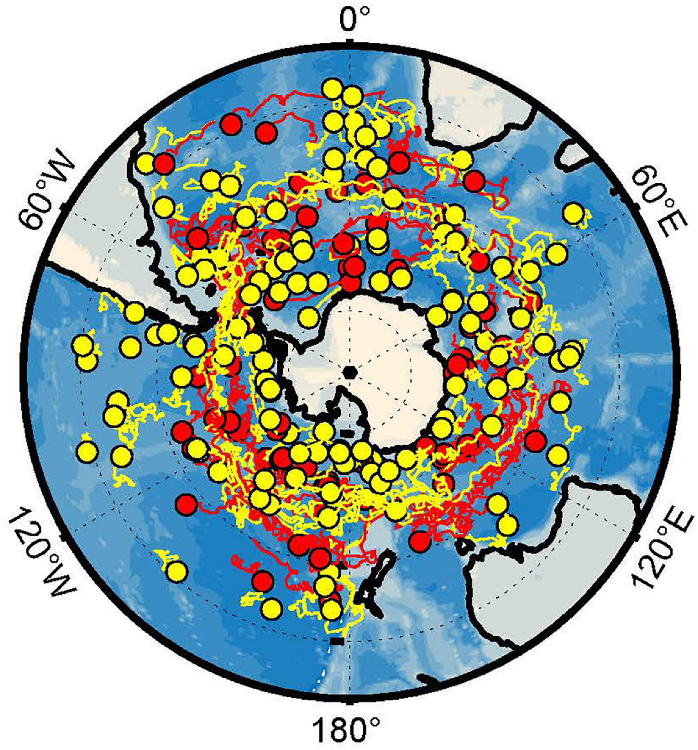
Figure 1. Current location (circles) and associated trajectories (lines) from floats within the SOCCOM array, as of December, 2020. Both operational (yellow) and inactive (red) floats are shown.

In contrast, in situ chemical sensors for measuring oxygen, nitrate, and pH on BGC-Argo floats represent newer technologies that require significantly more QC. Generally, the scientific use of raw, unadjusted BGC-Argo float data is not recommended. The real-time and delayed-mode adjustment processes greatly improve the quality of the BGC sensor data and result in a data set that is suited for research in a variety of applications. Various delayed-mode methods for BGC sensor recalibration and QC for oxygen, pH, and nitrate have been suggested (Johnson et al., 2013, 2015, 2017; Takeshita et al., 2013; Williams et al., 2016; Bittig et al., 2018a) but integrating the suite of methodologies into a coherent framework that can be used operationally across a fleet has proven challenging. Producing science-quality biogeochemical data requires consistent and traceable correction methods that can be adopted globally across all data centers involved in the processing and dissemination of BGC-Argo float data.

In this article we present the methodology developed as part of the SOCCOM program to assess oxygen, nitrate, and pH sensor gain, drifts and offsets in delayed-mode. The two accompanying MATLAB tools, SAGE (SOCCOM Assessment and Graphical Evaluation) and SAGE-O₂, are also described. The magnitude of required adjustments within the SOCCOM array and an independent validation of the described methods are also discussed.

SOCCOM Float Array

The SOCCOM array of profiling floats includes both Teledyne/Webb Research (TWR) APEX and Sea-Bird Scientific (SBE) Navis floats. All SOCCOM floats utilize Iridium two-way satellite communication and are equipped with ice-avoidance software as described in Riser et al. (2018) (following the method originally developed by Klatt et al. (2007)). For profiles taken while under ice, geographic coordinates cannot be obtained so latitude and longitude are estimated through linear interpolation. All SOCCOM floats are programmed to perform the nominal Argo mission of 10-day profile frequency from a maximum depth of 2000 m with an interim park depth of 1000 m.

The Southern Ocean Carbon and Climate Observations and Modeling floats carry a suite of biogeochemical sensors for measuring dissolved oxygen, nitrate, pH, chlorophyll fluorescence, and optical backscatter [colored dissolved organic matter (CDOM) fluorescence is also measured by sensors onboard certain Navis floats]. Although delayed-mode QC of the bio-optical parameters is a current area of research, chlorophyll-a, backscatter and CDOM visualizations have not been integrated into the SAGE software and these sensors are thus not considered further in this article. For information on the real-time processing and adjustment of these parameters see Johnson et al. (2017) and (Schmechtig et al., 2015, 2016, 2017, 2018a, b). The processing of raw oxygen, nitrate and pH sensor data from SOCCOM floats follows the procedures outlined within Argo processing documentation (Johnson et al., 2018a, b, Thierry et al., 2018a). Oxygen, nitrate, and pH sensor models vary slightly between the two float platforms used in SOCCOM. The In Situ Ultraviolet Spectrophotometer (ISUS) nitrate (Johnson and Coletti, 2002) and Deep-Sea DuraFET pH (Johnson et al., 2016) sensors used on APEX floats are primarily built and calibrated at the Monterey Bay Aquarium Research Institute (MBARI). pH sensors manufactured at SBE are also deployed on APEX floats. These receive pressure and temperature calibrations at SBE, and a final pH calibration at MBARI. All other sensors (including the SBE pH sensor onboard Navis floats, Submersible Ultraviolet Nitrate Analyzer, and SBE63 optodes onboard Navis floats, and Aanderaa optodes onboard APEX floats) receive factory-calibration direct from the manufacturer. Both sensor categories (MBARI-calibrated or manufacturer-calibrated) can suffer from shifts in laboratory calibration leading to changes in performance that manifest as sensor offsets or drifts in the field. While the root cause of such a calibration shift is not always known, the methods described herein provide a robust means for correction.

Automatic QC procedures are applied in real-time to flag grossly erroneous data within the SOCCOM array. These tests roughly follow the Argo real-time tests for BGC data as outlined in Schmechtig et al. (2016). Figure 2 shows SOCCOM float tracks colored by data quality, which is a useful way to assess the regional coverage of “good” BGC sensor data within the Southern Ocean and aids in deployment planning. Points along a float track marked in purple represent profiles where the automated QC tests have marked 100% of the data “bad.” Of the three parameters shown, pH sensor data have the highest number of “bad” quality flags, at 32.52% of the data, with a large regional gap located in the Pacific. Note that historical data from inactive floats remain a valuable part of the SOCCOM dataset.

FIGURE 2

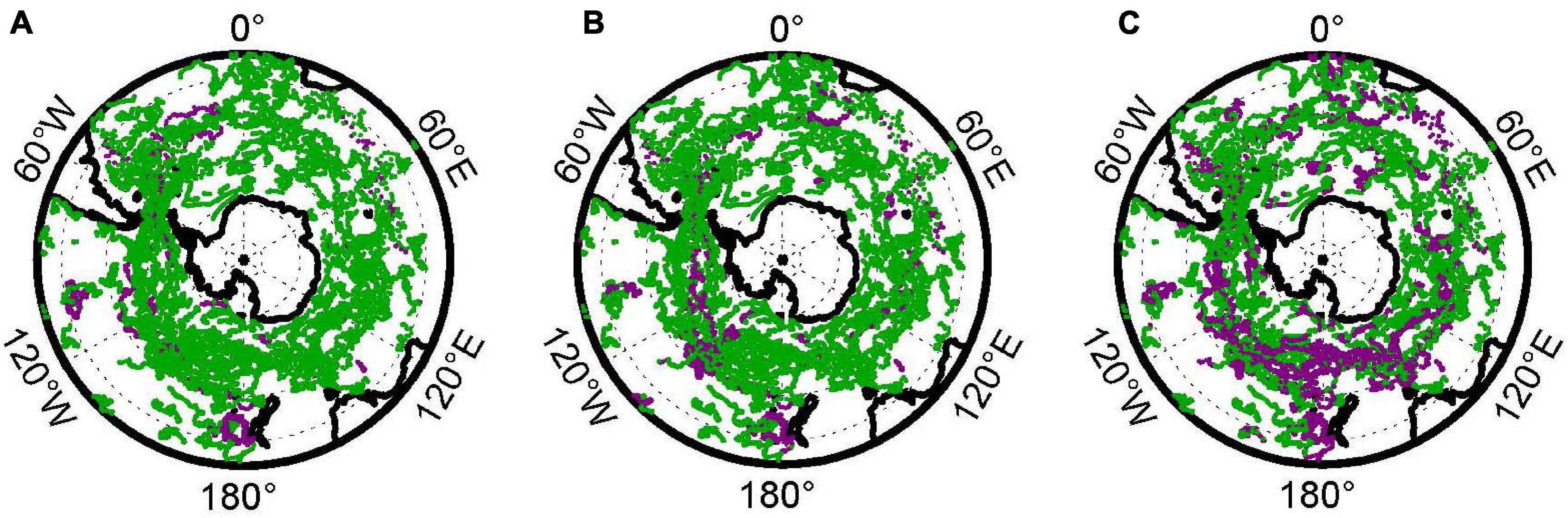
Figure 2. SOCCOM float tracks colored by data quality for (A) oxygen, (B) nitrate, and (C) pH. Points along a float track marked in purple represent profiles where 100% of the data has been marked “bad” by one of the automated QC tests. All other profile locations are indicated in green.

After passing the real-time quality checks, oxygen, nitrate, and pH data that are considered adjustable can be brought up to the accuracy level required for global biogeochemical studies through relatively simple correction procedures (Johnson et al., 2018b; Thierry et al., 2018b). This represents the second level of QC (Bittig et al., 2019). In the next sections, the delayed-mode procedures and accompanying software tools used to adjust oxygen, nitrate, and pH data from BGC-Argo profiling floats used by the SOCCOM program are presented.

Methods

Adjustment of Oxygen Data

The delayed-mode correction procedure for biogeochemical data on a SOCCOM float begins with oxygen. This is because the deep reference fields used in nitrate and pH QC (described in section “Reference Models Used in the Adjustment of Nitrate and pH Data”) are generated from empirical algorithms that require accurate oxygen measurements (along with other core variables and position information) as input parameters. Takeshita et al. (2013) have shown that the raw oxygen data from floats can be in error by as much as 20% of surface water oxygen saturation due to sensor drift during storage out of the water. Following Johnson et al. (2015), oxygen concentrations [(O₂), μmol kg^–1] can be corrected using a multiplicative gain factor, G, to improve the accuracy of a sensor suffering from the effects of storage drift [for additional information on optode storage drift see Bittig et al. (2018a) and D’Asaro and McNeil (2013)]:

$${\left[O_2\right]}_{corr}=G\times {\left[O_2\right]}_{raw}(1)$$

There is some evidence in the literature that a slope correction on oxygen concentration could potentially be improved by the inclusion of an intercept, especially in regions of near-zero oxygen levels (Bittig and Körtzinger, 2015; Bushinsky et al., 2016; Drucker and Riser, 2016; Nicholson and Feen, 2017). However, such corrections appear to be small (<1 μmol kg^–1), based on an assessment of 20 floats in the Arabian Sea and Bay of Bengal (Johnson et al., 2019) and are thus not implemented within the SOCCOM program.

SAGE-O₂ is the MATLAB Graphical User Interface (GUI) developed at MBARI to assist in deriving oxygen optode gain corrections by comparing oxygen data from a float to various reference datasets, including reanalysis values of oxygen partial pressure in the atmosphere. Images of the interface, including plot displays and user-controlled sidebars are shown in Figure 3 for SOCCOM float 9752 (WMO 5904694) in the Southwest Pacific, east of New Zealand. The top panel of each interface displays a time series of float data (blue) in comparison to the user-selected reference (red). The user can select whether to display raw float data (“RAW” tab, Figure 3A) or float data that has been adjusted using coefficients derived through the software (“QC” tab, Figure 3B). Details related to the calculation of the gain factor, G, over the lifetime of a float, as implemented through the software, are described further below.

FIGURE 3

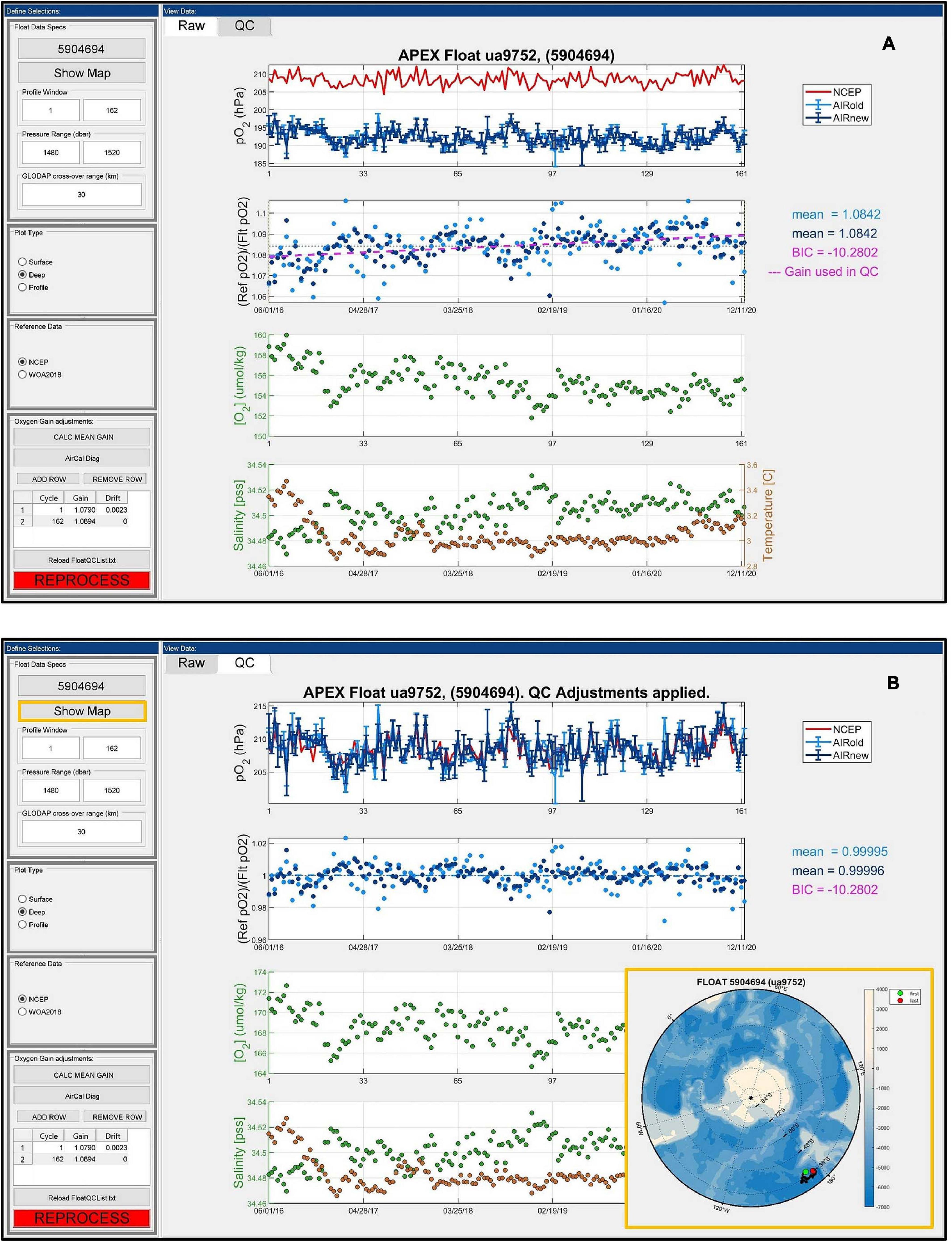
Figure 3. SAGE-O₂ software interface showing results of the calibration for sample float 9752, WMO 5904694. The view in (A) displays the raw oxygen float data against the reference, while the view in (B) displays float data that was adjusted using the coefficients derived through the software. The map display functionality is also indicated in (B).

Gain Computation Using In-Air Measurements

In-air calibration of oxygen optodes onboard profiling floats has been shown to bring accuracy to within 1% and is currently the operational standard (Johnson et al., 2015). For floats with in-air measurement capabilities, an estimate of atmospheric pressure must be available to compute the local oxygen partial pressure. The product referenced for oxygen gain computation within the SAGE-O₂ software is NCEP/NCAR Reanalysis-1 six-hourly surface pressure (Kalnay et al., 1996). This is a Gaussian gridded product with units of Pascals, which are converted to hectopascals (millibar equivalent) prior to proceeding. The NCEP atmospheric surface pressure (P_NCEP) values are interpolated to the time and location of the float’s surfacing. Values are then converted to oxygen partial pressure (p_{O_2}) based on the assumption that the atmosphere is 100% saturated with water vapor at the sea surface (Equation 2). The water vapor pressure (p_{H_2O}, in hPa) is calculated using Equation 3, where T represents temperature from the float in degrees Celsius (Aanderaa Instruments, 2017).

$$p_{O_2}=\left(P_{NCEP}-p_{H_{2}O}\right)\times 0.20946(2)$$

$$p_{H_{2}O}=e^{\left[52.57-\left(\frac{6690.9}{T+273.15}\right)-4.681\times ln\left(T+273.15\right)\right]}(3)$$

The sensor gain that is estimated from air oxygen for each individual profile, i, is then computed using Equation 4, as outlined in Johnson et al. (2015):

$$G_i=p_{O_{2}NCEP}/p_{O_{2}FLOAT}(4)$$

where p_{O_2NCEP} follows from Equation 2 and p_{O_2FLOAT} is the partial pressure of oxygen computed from the float (reported in millibars). The overall gain factor, G, used to correct all in water oxygen observations is then the mean of the n individual G_i values.

Mean gain values over the float’s life are displayed within the SAGE-O₂ interface in blue to the right of the plot panels (Figures 3A,B). Note that at the start of the SOCCOM program, APEX floats were programmed to take a single in-air oxygen reading with each surfacing that was associated with the telemetry phase of the cycle. A subsequent upgrade to the mission programming was initialized such that the optodes on APEX floats take a sequence of 8 in-air measurements at each surfacing at the end of ascent. Therefore, the majority of APEX floats in the SOCCOM program have two sets of in-air measurements: the original one associated with the telemetry phase (light blue in the GUI interface, labeled “AIRold”), and another larger set associated with the in-air measurement series (dark blue in the interface, labeled “AIRnew”). Both of these are plotted in the GUI for comparison. Average gain between the two sets differs by less than 0.1% fleet-wide.

Additional reanalysis products from other centers are also available, including the now real-time NCEP/DOE-R2 and the European Centre for Medium-Range Weather Forecasts (ECMWF) ERA5 reanalysis. The ERA5 product utilizes a more state-of-the-art (4D-variational) data assimilation system but its data latency (3 months lag for quality assured updates) may limit timely delayed-mode QC operations. In the future, the SAGE-O₂ software may be upgraded to utilize additional reanalysis products. The absolute uncertainty in reanalysis surface pressure fields from different products can be difficult to fully quantify. However, a comparison of NCEP and ECMWF operational models by Salstein et al. (2008) found that rms differences between surface pressure and shipboard observational stations were between 2 and 5 hPa in Southern latitudes with minimal difference between the two products, especially in more recent years. Surface pressure uncertainties of this magnitude roughly translate to less than 0.5% change in corrected O₂ measurements on individual floats.

Gain Computation Using Shipboard Bottle Data

The SBE63 optodes onboard SOCCOM Navis floats are plumbed in line with the pumped CTD flow stream and are thus not fully exposed to ambient air during surfacing. Thus, in situ calibration of these floats is performed by comparing float data to high-quality Winkler titrations from shipboard samples taken at the time of float deployment. The Winkler oxygen data are generated primarily on GO-SHIP cruises or by research groups that regularly participate in GO-SHIP cruises and they are considered to be of a quality consistent with GO-SHIP measurements (Hood et al., 2010 state a target accuracy of 2σ less than 0.5% of the largest oxygen concentration found in the ocean). Comparisons of the float and bottle data can be viewed through the software (Figure 4). We focus on the upper 50 m near the surface where oxygen is close to 100% saturated and the vertical gradients are small. A comparison of average gain values derived using shipboard Winkler measurements versus in-air samples for 97 SOCCOM APEX floats shows a mean difference (float minus bottle) of −0.31% [standard deviation (SD) of 2.2%]. This is not a large systematic bias for Navis floats with SBE63 optodes, but should not be ignored when trying to resolve gradual long term trends within the array.

FIGURE 4

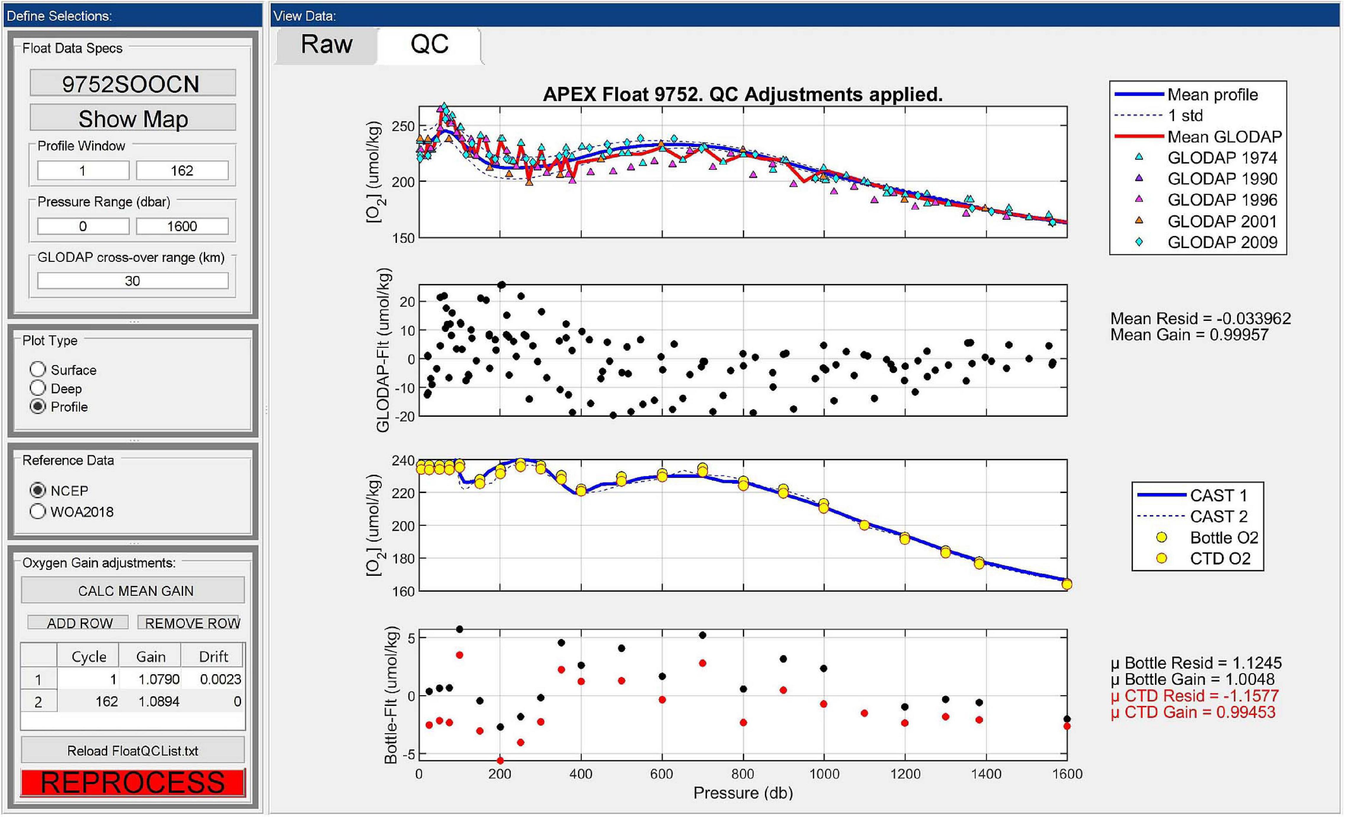
Figure 4. A comparison of adjusted oxygen data to GLODAPv2 (top two panels) and shipboard hydrocast matchups (lower two panels), as viewed through the SAGE-O₂ interface for UW/MBARI float 9752 (WMO 5904694).

In addition to providing an alternative approach to in situ optode calibration, comparison to shipboard data offers a simple and independent means for validating gain values derived from other methods, as described in sections “Gain Computation Using In-Air Measurements” and “Gain Computation Using Shipboard Bottle Data.” The gain correction for the float shown in Figure 3 was performed using in-air measurement data as described in section “Gain Computation Using In-Air Measurements.” Figure 4 shows data from this float in profile view. Pressure is along the x-axis for all plot panels. The top two panels show mean float data (solid blue line) along with Global Data Analysis Project v2 (GLODAPv2) profile data that are within a 30 km radius of the float data, and the computed residuals (note that the search radius can be modified by the user and is only applicable in profile view). The bottom two panels show the float’s first and second profiles (blue) along with shipboard Winkler and CTD oxygen data (circles), and computed residuals. Note that the “QC” tab is selected, thus all float data in the display have been adjusted using the computed gain shown in Figure 3. If the “Raw” tab was chosen, the float profile would have no adjustments applied. The small positive bias shown in reference to the bottle data is due to temporal mismatch between the shipboard data and float measurements within high-gradient regions of the profile. The mean residual (bottle-float) is 1.245 μmol kg^–1. The mean residual against all GLODAPv2 data within 30 km is −0.060 μmol kg^–1, although the range is larger than the hydrocast data due to the larger time range included in the matchup criteria.

Gain Computation Using World Ocean Atlas Climatology

For floats incapable of taking in-air oxygen measurements, and when shipboard reference data are not yet available, a preliminary optode gain correction factor can be derived within the SAGE-O₂ GUI using WOA percent oxygen saturation in surface water. This method follows Takeshita et al. (2013), which suggest an accuracy of 1–3% for sensors calibrated against WOA values. Percent saturation from the float is calculated following Equation 5 below. Solubility of oxygen (O_2Sol) is computed following section 1.3.3 in the Argo oxygen processing manual (Thierry et al., 2018a). Individual gain values, G_i, are then computed using Equation 6, where %Sat_WOA and %Sat_Float represent the mean WOA and mean float percent saturation values for the upper 25 m of the profile, respectively.

$$\%Sat=\left[O_2\right]/\left[O_{2Sol}\right]\times 100(5)$$

$$G_i=\%Sa{t}_{WOA}/\%Sa{t}_{Float}(6)$$

The overall gain factor, G, is calculated as the mean of the individual gain values (G_i) computed for each cycle. A comparison of gain factors computed using WOA percent saturation versus NCEP reanalysis air pressure as reference for 95 floats with in-air measurement capabilities shows a bias between the methods of 1.4% with a SD near 2%. The largest differences occur in floats near seasonal sea ice or very close to the coast where WOA reference climatology data are limited and/or seasonally biased. Note that for many floats within the global BGC Argo array, this method is the most accessible option for data managers and should be applied wherever possible as a first-order correction.

Drift in Optode Gain

The effects of pre-deployment storage drift are readily apparent across the majority of optodes used on profiling floats. Oxygen data from all Aanderaa and Sea-Bird optodes onboard SOCCOM floats require gain correction, with a fleet-wide mean gain correction of 7.0 ± 4.6 (1 SD) %. While an optode’s stability once deployed is substantially greater, it is less predictable (Bittig and Körtzinger, 2015, 2017; Johnson et al., 2015; Bushinsky et al., 2016). Bittig et al. (2018a) provides a thorough review on this topic, and suggests that individual optodes may exhibit significant post-deployment drift of up to ±0.6% year^–1. If not accounted for, such drift could lead to significant biases in certain biogeochemical analyses such as air-sea fluxes.

Characterizing the amount of optode drift is possible within the SAGE-O₂ software through comparison against reference values over time. This method was recently put into practice for select floats within the SOCCOM array. The software allows the user to auto-calculate the drift relative to a reference such as NCEP. The computed offset (initial gain), b, and slope (drift), m, are calculated using a model I regression of computed gain on each cycle against cycle time. For a float drifting since deployment, the gain value applied at each cycle (following Equation 1) then becomes:

$$G_{i=1:k}=b+m(\mathrm{△}T)(7)$$

where △T is the time, in years, elapsed since the first cycle. In situ optode drift is considered a slow process and a linear model is thought to best approximate sensor behavior (Bittig and Körtzinger, 2017). However, the software is flexible enough to support rare cases requiring a segmented drift correction. If the chosen ending node at cycle k is not the final cycle reported from the float upon assessment, a drift assessment on the subsequent segment (cycles i = k:n) is automatically performed. The slope of the second segment, m₂, is found by first subtracting the recomputed gain at the end of the first segment (G_k) from individual gains, g_i, of segment 2, and then regressing segment 2 through the origin. This can be expressed as

$$m_2=\mathit{\hspace{1em}}\frac{{\sum }_{i=k}^n\left(g_i-G_k\right)*x_i}{{\sum }_{i=k}^{n}x_i{}^2}(8)$$

where x represents the time elapsed since the ending cycle of segment 2. This method results in drifting gains that remain continuous throughout segments. However, note that drift assessment within the GUI (and especially multi-segment drifts) should be limited to advanced users. It is recommended that drift assessment be performed only after a sufficient amount of data has been received (optimally at least 2 years). Care must be taken in order to prevent correcting for an apparent drift that has been influenced by a seasonal cycle.

Within the GUI there are two methods to test whether or not a computed drift over the lifetime of a float is statistically robust. Upon auto-computation of the drift, a two-tailed T-test is performed to assess whether the calculated slope is significantly different than zero at the 95% confidence interval (results are returned on screen). Additionally, on the right-side panel in the interface (see Figure 3), the GUI reports the computed Bayesian Information Criteria (BIC) (Schwarz, 1978) following Equation 9 below, where SSR represents the sum of squared residuals of the model, K is the number of model parameters, and n represents the number of data points in the time series. The BIC weighs the number of predictors within a model against the goodness-of-fit, allowing the user to prevent over-fitting of the data (the model with the lowest BIC is always preferred).

$$BIC=\log \left(\frac{SSR}{n}\right)+\frac{K\log n}{n}(9)$$

In the SOCCOM array, of the 126 floats currently considered candidates for optode drift correction, 32 exhibited significant drift rates. Both positive and negative drift rates were observed, with a mean of −0.07% per year, a SD of 0.65% per year and a total range of −1.1 to 1.2% per year.

The drift correction proposed here relies on the existence of air oxygen measurements relative to the NCEP atmospheric reference. However it does not address the root cause of sensor drift behavior which is somewhat unsatisfying. Bittig et al. (2018a) show how inadequate temperature calibration of the oxygen optode can oftentimes account for in situ drift rates apparent in a float’s optode time series. They describe a correction method (equation 23 of referenced publication) that can simultaneously correct for inadequate temperature calibration and any seawater carryover on the sensor during sampling while in air. The supplementary material to their paper highlights the results of applying the method to UW/MBARI float 9313 (WMO 5904474); the strong oxygen-temperature response exhibited by this float is shown to bias the sensor gain time series and application of the correction method effectively removes the apparent drift in sensor gain. However, recent testing demonstrates that this correction approach may not be applicable across the full SOCCOM array. Figure 5 plots computed drift in optode gain against the residual drift in optode gain after temperature compensation using equation 23 from Bittig et al. (2018a) is applied for 82 SOCCOM floats that have been operational for at least 2 years. A Model II regression (shown in red) gives an offset of 0 which suggests that the Bittig et al. (2018a) correction is robust and does not add spurious drift. The slope of the Model II regression is 0.797 (different than 1 at the 99% significance level) suggesting that across the SOCCOM array, the correction reduces the apparent drift in gain by 20.3%. For certain floats, the Bittig et al. (2018a) correction tends to underestimate the magnitude of the true drift of the optode, suggesting that error in the temperature calibration of the optode is not the only potential mechanism affecting optode drift and additional drift correction may be warranted. The mean difference in gain drift before versus after the correction is −0.021% per year and the SD of the differences is 0.319% per year. These results highlight the fact that the optode-temperature response is unique to each sensor. This result is in accordance with findings of Johnson et al. (2017) who show that only 20% of the change in gain over time can be accounted for by temperature changes observed by a float. Such corrections should therefore not be applied systemically across the whole fleet, but rather integrated on a float-by-float basis in delayed-mode with statistical indexing to weigh the benefit of added complexity of the correction, similar to what is currently being done to assess the need for drift corrections. These methods may be integrated into the GUI framework in a similar manner in a future revision.

FIGURE 5

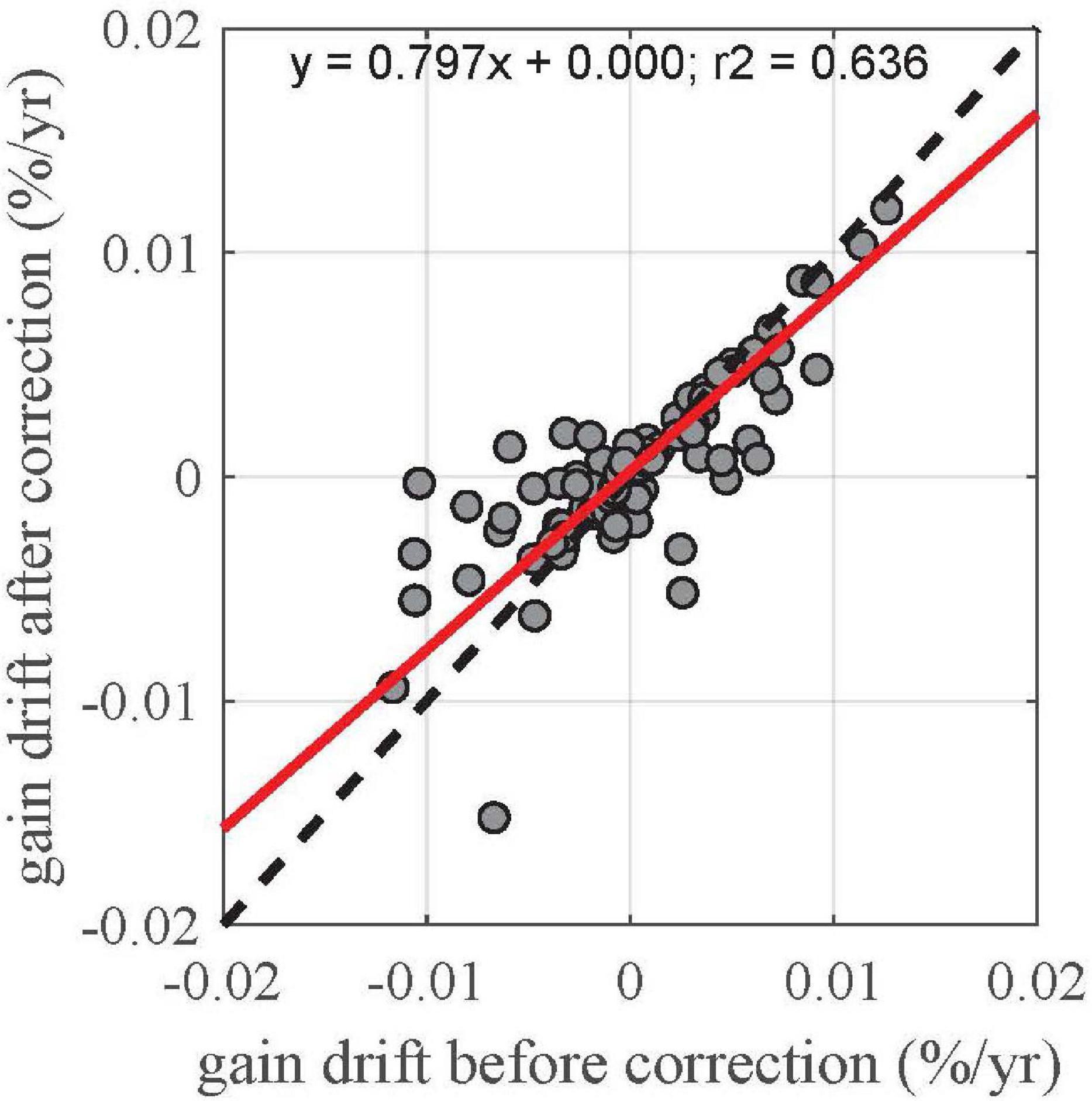
Figure 5. Comparison of post-deployment optode drift before and after application of Bittig et al. (2018a, equation 23). Analysis includes 82 SOCCOM floats. Dashed line depicts the 1:1 relationship; red line is a Model II regression (uncertainty in both X and Y).

Adjustment of Nitrate and pH Data

Adjustment of nitrate and pH data are performed after oxygen data has been corrected. Similar to oxygen optodes, nitrate, and pH sensors on profiling floats often suffer from initial calibration shifts that must be corrected prior to scientific use. Such inaccuracies can manifest as offsets and/or drifts throughout the data series. As described in Johnson et al. (2017), pH offsets and drifts can be attributed to changes to the sensor reference potential (k₀) over time, while those apparent in nitrate usually result from changes in light throughput due to aging or fouled optical components. Therefore, adjustments to pH and nitrate are applied as offsets to k₀ and nitrate concentration (μmol kg^–1), respectively.

The general adjustment process for pH and nitrate is based on evidence that the offsets and drifts are constant throughout an entire profile (Johnson et al., 2013, 2017). For example, Johnson et al. (2013) show that deviations of surface nitrate from zero are paralleled at depth (1000 m) for a profiling float near station Hawaii Ocean Timeseries; offsets derived at the surface applied to the entire profile yielded corrected data within 1 μmol kg^–1 of reference at 1000 m depth. Corrections for SOCCOM floats involve comparison of raw float data to select reference fields at depths below 1000 m (1500 m is the default target depth used in SOCCOM operations) where spatial and temporal variability in ocean chemistry is minimal. The corrections determined at depth are then applied to the entire profile. This process is similar to the protocol used to correct Argo salinity data (Owens and Wong, 2009). Figure 6 below shows the SAGE GUI interface where such comparisons can easily be performed. Upon selecting a float, default view specifications are loaded into the GUI, including a profile window encompassing the entirety of the float’s life-span, and a pressure range of 1480–1520 m where adjustment assessment is performed (although this depth range can be adjusted by the user). Float (blue) and reference (red) data within selected time and pressure ranges are plotted in the top panels, and the anomaly series (float minus reference) is plotted below in green (see section “Reference Models Used in the Adjustment of Nitrate and pH Data” below for a description of optional reference datasets). GLODAPv2 (Olsen et al., 2020) crossover data are also shown in the upper panel plots as a climatological reference, but only to assess the consistency of adjusted data. As in SAGE-O₂, the search distance for GLODAPv2 data from each profile can be set in the GUI.

FIGURE 6

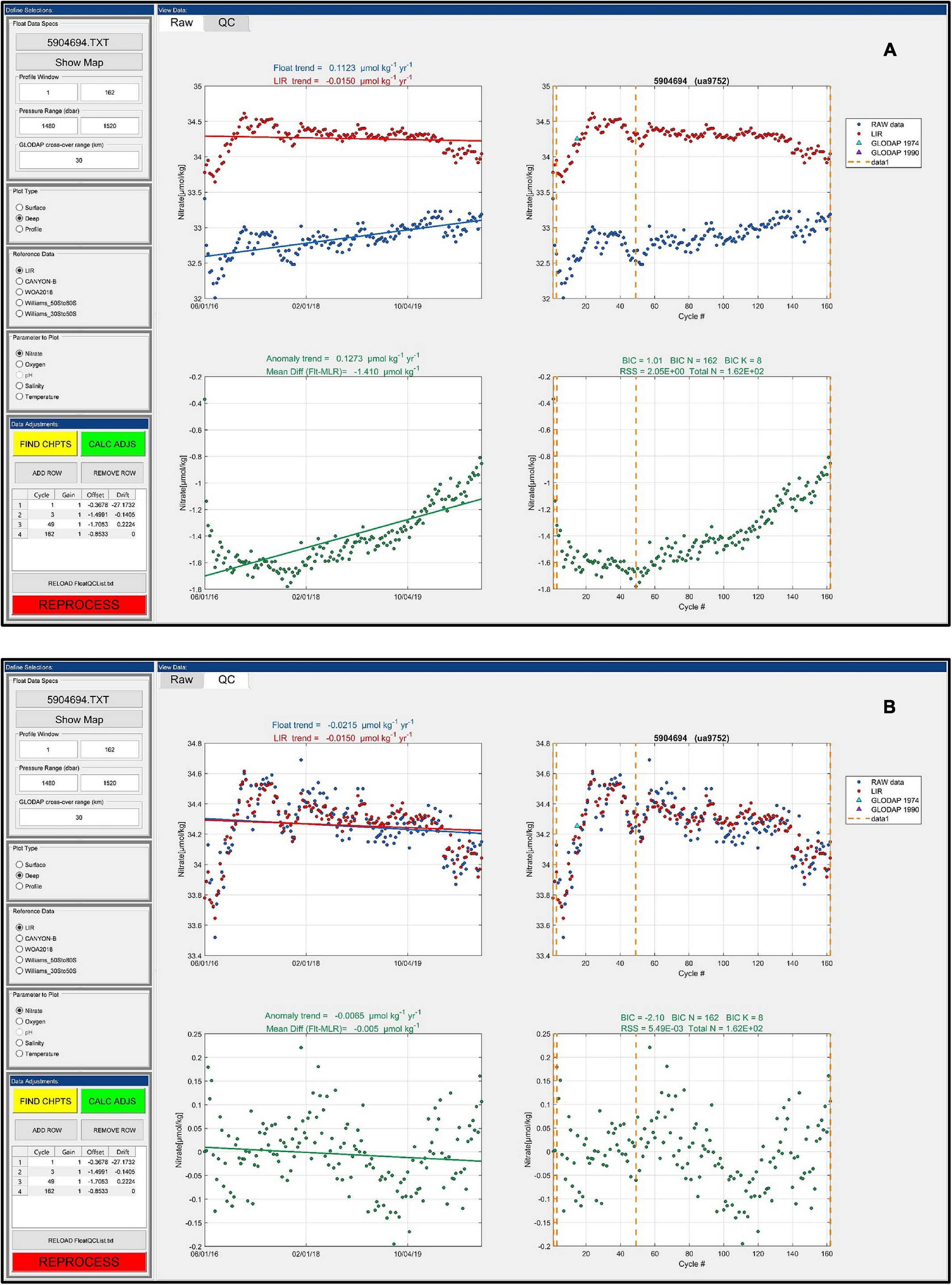
Figure 6. SAGE software interface showing nitrate data (blue) from MBARI/UW float 9752 (WMO 5904694) against the selected “LIR” reference (red) and the resulting float minus reference anomaly time series (green). The view in (A) displays the raw nitrate float data; the view in (B) displays nitrate data that has been adjusted using coefficients derived through the software.

Similar to conductivity sensors (Owens and Wong, 2009), drifts and offsets occurring in data from nitrate and pH sensors often vary linearly over long time periods, but calibration jumps in the time series are not uncommon. Oftentimes the largest drift rates occur over the first few cycles in a float’s life as can be seen in the nitrate anomalies shown in Figure 6A. Nitrate and pH anomalies from a float data series are thus best modeled as discontinuous piecewise linear fits, where both drifts and offsets change independently between segments that are bounded on either side by defined cycle breakpoints. In the Figure 7 schematic, the correction, ΔANOM, at each cycle breakpoint, j, is calculated as

FIGURE 7

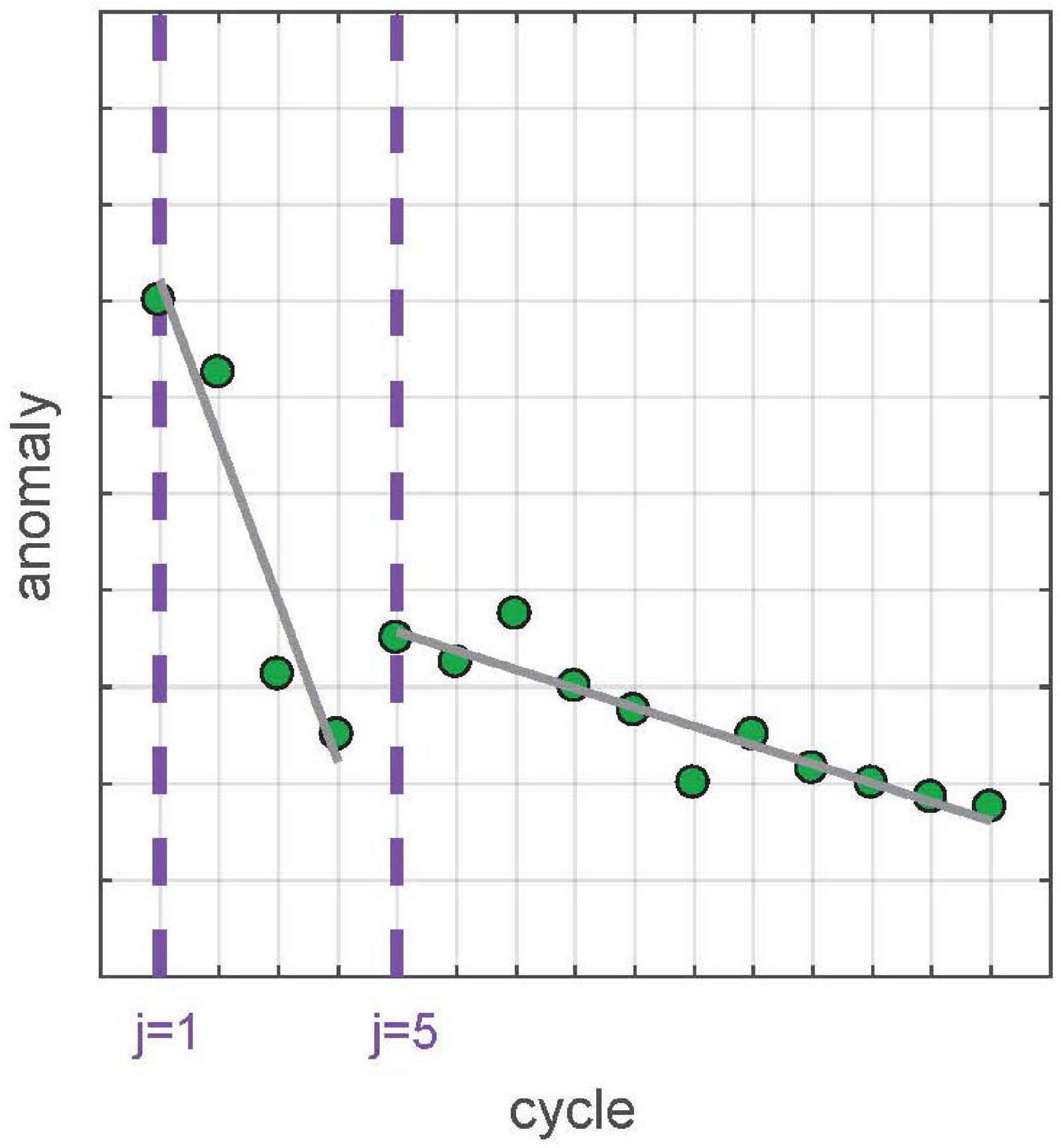
Figure 7. Qualitative schematic showing the adjustment model of a theoretical sensor anomaly series. The two series breakpoints, identified in purple, occur at cycles 1 and 5. Gray lines represent the least-squares fit (adjustment model) to the elements (green dots) within each segment.

$$ANO{M}_j=O_j(10)$$

and the data correction for any subsequent cycle, i, within the same segment becomes

$$ANO{M}_i=O_j+D_j\left(T_i-T_j\right)(11)$$

where O and D represent the offset (in μmol kg^–1) and drift (in μmol kg^–1 per year), respectively, of the linear least squares fit to the anomaly data series between cycles located at breakpoints j and j + 1 (not including the latter bounding breakpoint), and T represents time (in years). For nitrate data, this modeled correction (represented by gray lines in Figure 7) is then subtracted from the original data series. For pH data, the modeled correction is applied as an offset to the reference potential (k₀) of the sensor as described in Johnson et al. (2016). Note that Johnson et al. (2018b) describe a correction that is applied as a pH offset at the depth where the anomaly was determined, rather than a reference potential offset. The correction in Johnson et al. (2018b) is conceptually incorrect and adjustments should be made to k0, although as implemented in Johnson et al. (2018b) the results were nearly identical. A matrix of correction factors (as shown in the lower left corners of Figures 6A,B) is stored in a float-specific text file along with any derived oxygen corrections for use in reprocessing applications. This method constitutes a delayed-mode correction approach that can be revisited and characterized at periodic intervals throughout the float’s life.

Reference Models Used in the Adjustment of Nitrate and pH Data

Multiple options are available for use in the estimation of deep pH and nitrate reference fields for comparison against float data. These include World Ocean Atlas climatological fields as well as empirical algorithms derived from high-quality shipboard data acquired from GO-SHIP cruises (Williams et al., 2016; Bittig et al., 2018b; Carter et al., 2018). While the algorithms provide estimated fields rather than direct measurements, their performance has been extensively validated. The set of multiple linear regression models (MLRs) by Williams et al. (2016) were the first of such reference algorithms available in the Southern Ocean and were utilized in the QC of SOCCOM nitrate and pH float data during the early years of the program. Nitrate and pH estimates produced using the Williams method rely on MLR equations specific to two latitudinal bands around the Southern Ocean. Predictor variables include pressure, salinity, temperature, and oxygen. A key distinction between the Williams MLRs and the other methods available for use within the SAGE software is the lack of global extent in the Williams MLRs. In addition, this method is limited in depth space to the range of 1000–2100 m. While this fully encompasses the depth nominally used in QC for the majority of SOCCOM floats, sometimes shallower reference depths are required, for example when a float is under-ballasted and cannot reach 1000 m. Nonetheless, the Williams MLR algorithms perform very well when used within their specific range limits. Williams et al. (2016) states root mean square errors (RMSE) of 0.3 μmol kg^–1 and 0.004 total pH units for deep (1500 m) nitrate and pH estimates, respectively. Additionally, Johnson et al. (2017) show linear regressions between first nitrate and pH profiles from SOCCOM floats, adjusted to the Williams MLRs at depth, and shipboard bottle data taken at the time of deployment to be near unity, with midrange differences (bottle minus float) of −0.1 μmol kg^–1 and 0.006 pH units, respectively. These findings validate the method as an acceptable reference option for float programs in the Southern Ocean.

However, as increasing numbers of BGC floats are being deployed outside of the Southern Ocean, an alternative reference algorithm with full global extent is now the operational standard. This allows for a consistent procedure, homogenous across float arrays. The current default choices for estimating nitrate and pH for comparison against SOCCOM float data are the locally interpolated nitrate regression (LINR) and the locally interpolated pH regression (LIPHR) (or LIRs, collectively) (Carter et al., 2018). The LIR algorithms were developed from a series of MLRs trained using GLODAPv2, resulting in a separate set of coefficients for each 5° latitude and longitude grid box and 33 different depth surfaces. The derived coefficients at each grid point then get interpolated onto a float’s location for use in generating a final nitrate or pH estimate. For SOCCOM assessments, depth, salinity, temperature, dissolved oxygen as well as profile latitude and longitude are used as predictor variables (LIR regression #7). The RMSE of the residuals between LIPHR and LINR estimates within 1000 and 2000 m using predictor set #7 and the test observations used for algorithm validation were 0.006 pH units and 0.47 μmol kg^–1, respectively (Carter et al., 2018).

A third optional reference algorithm is the CArbonate system and Nutrient concentration from hYdrological properties and Oxygen using a Neural-network, Bayesian approach (CANYON-B, Bittig et al., 2018b). This is a neural network mapping performed in a Bayesian framework, that is, informed by an ensemble of model components at each stage rather than fixed values. This model is a revised version of an earlier individual neural-network approach, CANYON, originally developed by Sauzède et al. (2017). In their publication, Bittig et al. (2018b) compare the performance of CANYON-B with LIR for various parameters, including nitrate and pH, against a post-GLODAPv2 validation dataset. The authors stress that, while both methods perform similarly well in a bulk statistical sense, local estimates can still be quite different. Figure 8 compares differences between pH and NO₃^– estimates for the SOCCOM array using CANYON-B and LIR algorithms. The mean (SD) of the differences at the 1500 m depth level (the target depth for QC assessment in SAGE) are −0.001 (0.006) for pH and −0.053 (0.278) μmol kg^–1 for NO₃^–. Larger differences near the surface are largely due to greater uncertainty in the LIR algorithms at these depths, as is discussed in Bittig et al. (2018b) (see figure 3 and associated text from their publication). However, as is also noted by Bittig et al. (2018b), estimates from all algorithms show some level of enhanced uncertainty toward the surface due to difficulty in accurately capturing seasonal variability and effects of air-sea gas exchange. It should be noted that pH estimates generated by CANYON-B are intended to be in line with pH calculated from DIC and TA, whereas pH estimates using the LIPHR method are considered to be consistent with pH that has been spectrophotometrically measured (for further discussion on the pH-dependent bias that exists between computed versus spectrophotometrically measured pH, please see Carter et al., 2018). While the LIPHR algorithm has a flag to apply a linear adjustment that will subsequently produce estimates consistent with calculated pH, this method should not be used for calibrating a pH measurement from a float, as ISFET pH is consistent with spectrophotometric pH measurements (Takeshita et al., 2020). The differences shown in Figure 8 were performed after a linear transformation was applied to CANYON-B estimates following Carter et al. (2018, equation 1) to bring estimates back into alignment with spectrophotometrically measured pH.

FIGURE 8

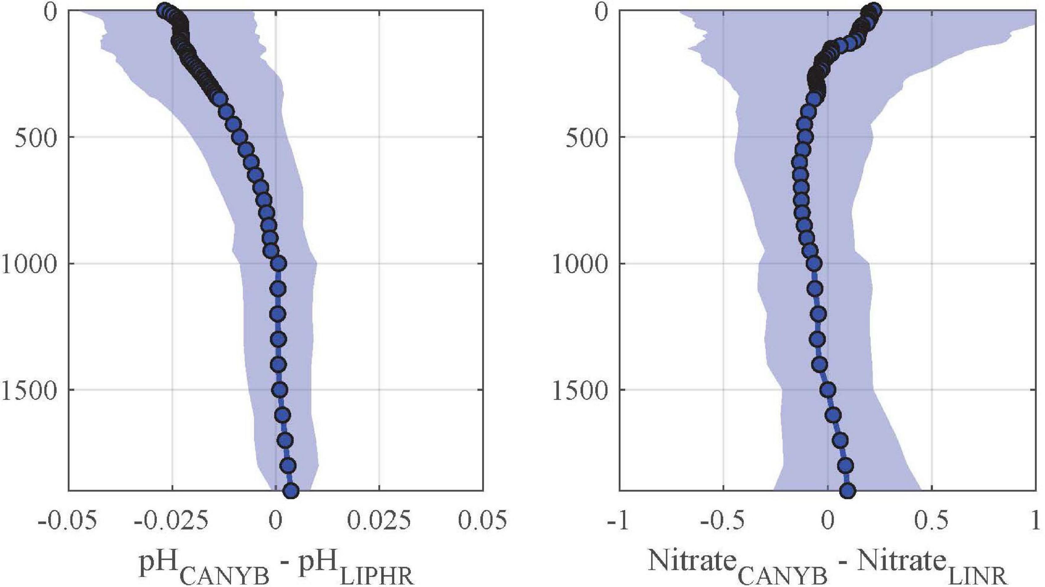
Figure 8. Fleet-wide differences of computed pH (left) and nitrate (right) using CANYON-B and LIR algorithms. Data were binned at 10, 50, and 100 m pressure intervals for 0–350, 350–1000, and 1000–2000 db, respectively. The blue line represents the median difference and the shaded areas represent the interquartile range.

A final note should be made regarding the use of pH estimates that are based on measurements made over a large time span. Ocean pH is decreasing due to increasing atmospheric carbon dioxide concentrations and these effects are sometimes detectable at the depth range used for pH sensor adjustment (Ríos et al., 2015). Each of the algorithms described here has been trained on shipboard data that may exhibit this effect. While the LIPHR algorithm does include a flag for optional application of an ocean acidification adjustment, this is a static adjustment and does not account for geographic differences in ocean acidification rates, nor does it account for changes in global ocean acidification rates over time. This highlights the need for such reference equations to be periodically updated, utilizing recent training datasets to provide more accurate algorithm coefficients.

Computation of Nitrate and pH Adjustments Using Automated Change-Point Detection

In the initial version of the SAGE software, the user manually chose the location of each breakpoint (node). The inherent subjectivity in this approach in addition to the increasing time investment required by the operator to complete a full adjustment assessment of the SOCCOM array proved less than optimal. In the current software version, both the optimal number and location of each breakpoint can be assigned automatically through an automated multi-step process. First, the binary segmentation method of change-point detection is applied using the MATLAB function, ischange, which begins by splitting the data series for variable y, of length n, into two segments separated by a change-point, j (Killick et al., 2012). The location of j along the time series is then iteratively shifted until a minimization of the left side of the following equation is reached:

$$C\left(y_{1:j}\right)+C\left(y_{\left(j+1\right):n}\right)<C\left(y_{1:n}\right)(12)$$

where C represents the cost function

$$C\left(x\right)=nVar(x)(13)$$

where n is the number of data points in the segmented data series, x, and Var is the variance. This process is then repeated, further splitting up the segments to find the optimal location of an increasing number of changepoints. Next, in order to statistically determine the best number of changepoints of the various groupings tested, a modified BIC is calculated for each model, following

$$BIC=\log \left(\frac{SSR}{n}+{\alpha }^2\right)+\frac{K\log n}{n}(14)$$

where the α term is used as a threshold on the mean residual, driven by the target accuracy of the sensor. In SOCCOM processing operations, α = 0.5 and α = 0.005 are used for nitrate and pH data, respectively. If α is omitted, equivalent to assuming the sensor has no inherent noise, the changepoint algorithm will often find an excessive number of change points, which is inconsistent with known sensor behavior. The location and number of changepoints from the model with the lowest BIC value is then used to derive offsets and drifts as described in section “Adjustment of Nitrate and pH Data.” Note that the presence of NaNs (missing data) along the BGC data series prohibits the auto-calculation of change-points, so any missing values are first linearly interpolated. In an attempt to encourage the operator to more carefully scrutinize a data series with large amounts of missing data (in the case of a poorly performing sensor or shoaling float), a warning message will pop-up if more than 50% of the BGC data series is missing. However, this is only a safeguard and does not necessarily mean that the auto-changepoint detection method is not applicable.

A key concern in the move from a manually assigned to an automated definition of breakpoints in the sensor QC-adjustment process was the potential for degradation in accuracy of the adjusted SOCCOM dataset. Thus, prior to operational implementation of the automated method, a quality assessment was performed using two adjusted datasets, one done manually by a trained biogeochemical float QC operator and the other performed automatically using the changepoint detection method described above. Figures 9A–D show that the use of automated changepoint detection in the SOCCOM QC process results in a fewer number of change-points, on average, and an overall better model of the anomaly time series, in a statistical sense (lower BIC value), than the previously employed manual correction method.

FIGURE 9

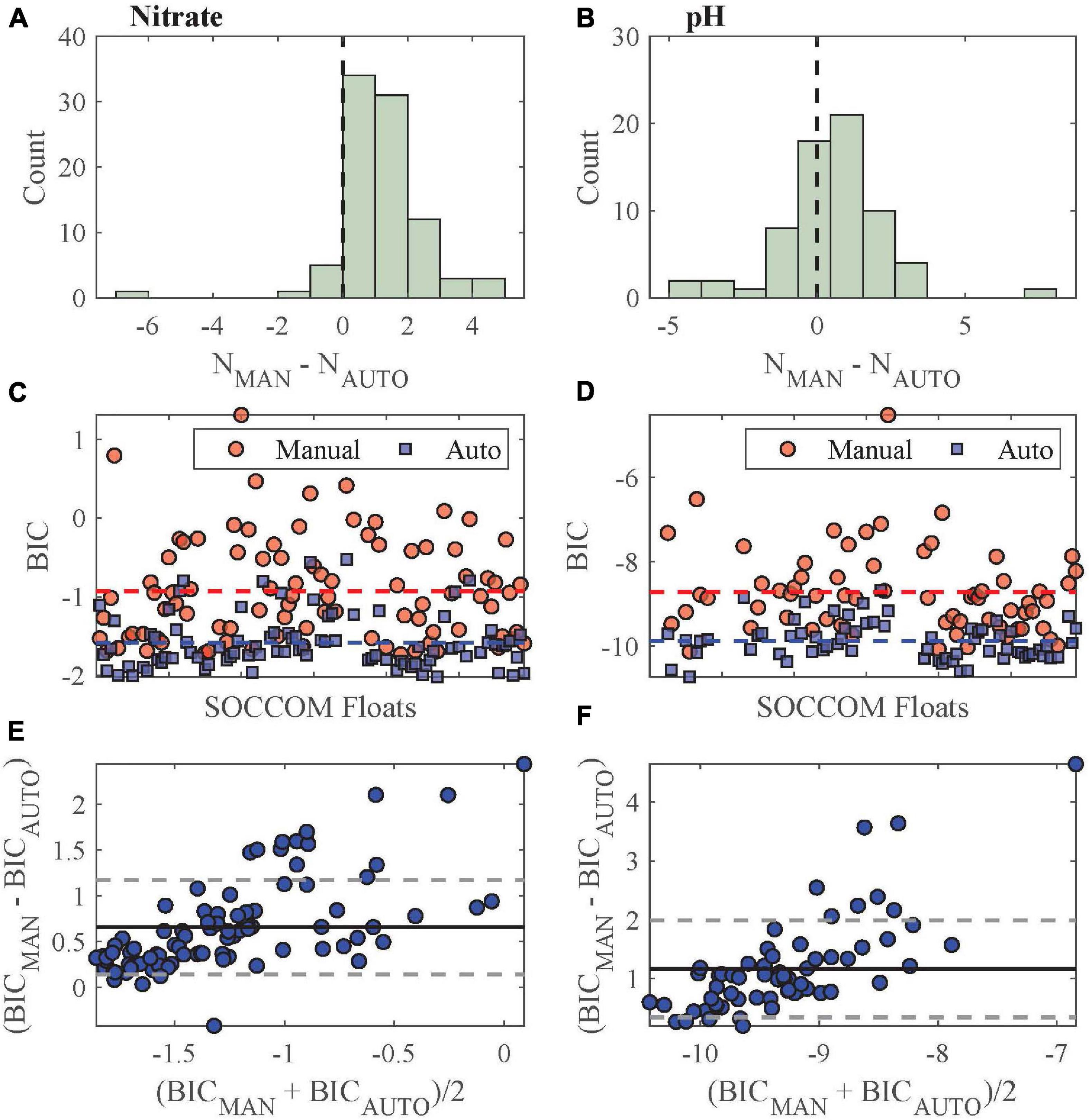
Figure 9. (A,B) Histograms showing differences in number of changepoints identified by the manual (N_MAN) versus automated (N_AUTO) method for nitrate and pH sensor QC. (C,D) Comparison of computed Bayesian Information Criterion (BIC) for manual (red circles) and automated (blue squares) changepoint identification in nitrate and pH QC. Dashed lines represent mean BIC values for each method. (E,F) Difference in computed BIC (manual versus auto) against mean BIC value for each float, for nitrate and pH. Solid and dashed lines represent mean difference ±1 SD, respectively. A total of 120 SOCCOM floats were used in each analysis.

However, the absolute difference in BIC between models is small in most cases (mean differences of 0.658 and 1.165 for nitrate and pH, respectively) with the automated method showing progressively better performance as model complexity increases (Figures 9E,F). It is generally accepted that when comparing candidate models, a difference in computed BIC less than 2 is relatively inconsequential, meaning that the two models are statistically similar and minimal (if any) improvement can be attained by choosing one over the other (Kass and Raferty, 1995; Fabozzi et al., 2014). When taken in this context, results from this comparison suggest that the initial manual method of change-point detection for QC across the SOCCOM fleet was not of poor quality, and that the move to automated changepoint detection sustains such quality while concurrently reducing the time required to perform an objective fleet-wide assessment.

Results

Nitrate and pH Adjustments Applied to SOCCOM Float Data

The magnitude of a required sensor adjustment, as derived from the methods described in the previous sections, represents the degree to which sensor performance has changed since laboratory calibration. A summary of the adjustments required over time across a full array of sensors can unveil any systematic biases and subsequently help identify key areas for which to focus future development efforts. While the adjustment methods described in this article improve data accuracy, reducing the magnitude of required adjustments to a sensor (through ongoing improvements to sensor design) is the optimal goal. As described in section “Adjustment of Nitrate and pH Data,” the coefficients to the linear fits of each segmented anomaly series are included within a single float-specific correction matrix that is used in the data adjustment process. The offset associated with the first segment exemplifies sensor performance upon deployment. As each segment is treated independently, the value of any subsequent offset can provide information on sensor health over time when viewed relative to the first offset.

The distributions of the first and second offsets required for nitrate and pH data in the SOCCOM array are shown in Figure 10. The positive skew of the nitrate first offset distribution demonstrates that the majority of SOCCOM nitrate sensors are biased high upon deployment while the opposite is true for pH sensors within the array. The magnitude of the bias is 0.91 μmol kg^–1 for nitrate, and −0.032 for pH (Table 1). Distributions of the second offsets (relative to the first) show reduced spread across both sensor types and an elimination of bias in pH sensor data. This behavior is not surprising; oftentimes the largest anomaly is observed on the first cycle as the sensor re-conditions to an aqueous environment. Continued exposure to seawater at 1500 m helps to stabilize the sensors, particularly the pH sensor. The optics of the nitrate sensor are more sensitive to transient perturbations induced by biofouling so jumps in the data series are more often observed. This is exemplified by the fact that a small bias (negative) remains in the distribution of second nitrate offset, showing that a second offset is almost always required to bring nitrate data in line with climatology.

FIGURE 10

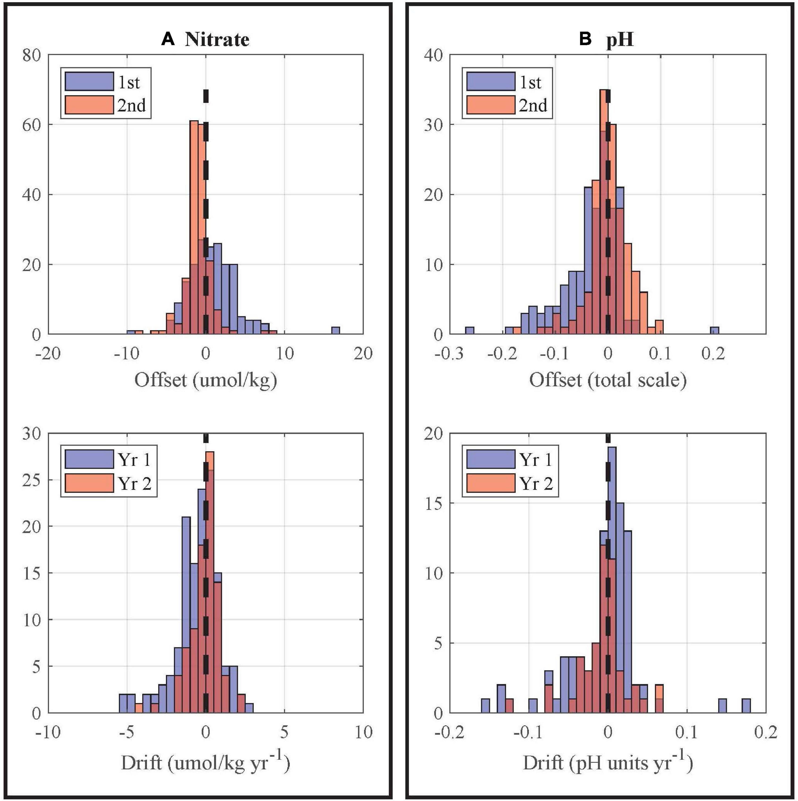
Figure 10. Histograms of first and second offsets (top), and first-year and second-year drift rates (bottom) for nitrate (A) and pH (B) data. Offsets were computed as float data minus reference data at a nominal calibration depth of 1500 m; the second offset is relative to the first. Drift rates were computed using a Model I regression on the anomaly time series.

TABLE 1

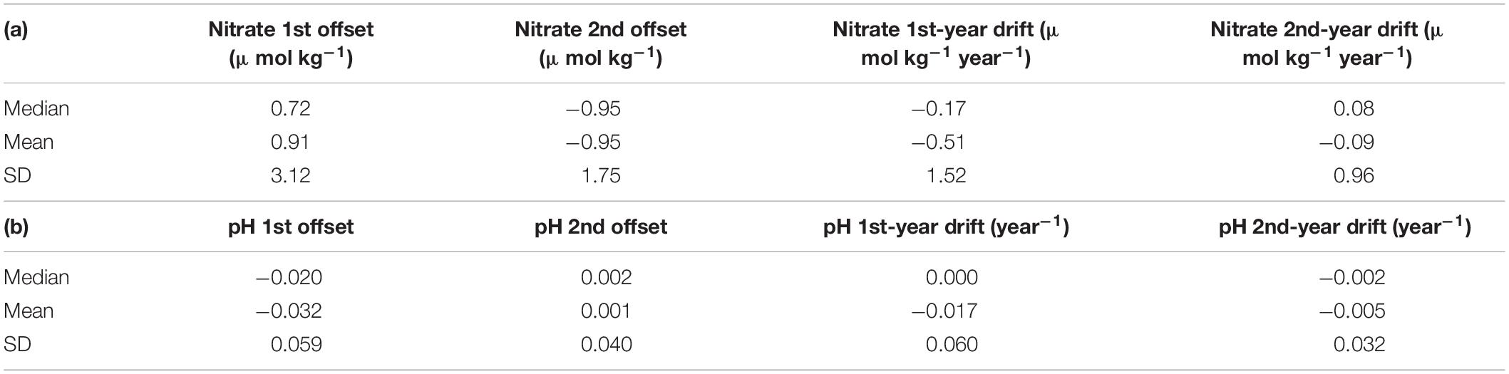
Table 1. Data adjustment summary statistics for nitrate (a) and pH (b).

Also notable in the distributions is that there is a small subset of floats receiving relatively large first offset corrections for nitrate and pH sensor data. Currently there is no operational threshold in place for maximum allowable adjustment. Floats requiring larger than normal nitrate or pH adjustments are analyzed on a case-by-case basis and may be gray-listed as bad or questionable by the delayed-mode operator upon review of laboratory calibration and sensor diagnostics. These large offsets may be the result of changes in optical alignment or sensor contamination during transport.

First year and second year sensor drifts for nitrate and pH are also shown in Figure 10 (lower histograms). These were computed as the slope of a Model I regression over the first and second year of data for each float. This ensured a uniform time frame for drift comparison across the array (as the length of each segment within a float’s adjustment matrix can vary). While drift in the second year is not completely eliminated, there is an 80% (70%) reduction in mean drift rate across the array for nitrate (pH) sensors from year 1 to year 2. The reduction in sensor drift from year 1 to year 2 is not a uniform rate of change. By the second year, around 25% of nitrate anomalies have drifted beyond 2 μmol kg^–1 of their initial value with the majority of sensors drifting negative (measuring low relative to reference fields) and the largest proportion of drift occurring within the first five cycles. pH sensors see both positive and negative drift rates, with close to 50% of the data drifting beyond 0.03 pH units of their initial value. However, similar to nitrate sensors, pH sensors are also relatively stable beyond the first few cycles. Because both nitrate and pH sensors exhibit the largest rates of in situ drift within the first 2 months since deployment, it is recommended that initial QC assessment be performed only after the first five cycles have been returned from a float.

While we see sensor stability improving with time since deployment for individual sensors, it is also important to understand if adjustment requirements across the array are improving over each subsequent deployment year. Figure 11 shows box plots of the first offsets required for nitrate (left) and pH (right) data grouped by deployment year. Median offsets for nitrate seem to be more or less randomly distributed around zero, indicating that the mechanisms responsible for post-deployment shifts in calibration are somewhat poorly constrained. For pH, this is not the case. Median values remain negative over all deployment years which suggests a systematic negative bias for this sensor. pH sensor offset statistics also show a more dramatic change over time, in both the location of central tendency and degree of dispersion. These shifts in offset statistics are likely linked to changes in sensor design or laboratory calibration procedure. For example, significant improvements were seen in 2016 due to the implementation of improved pH sensor conditioning protocols in the lab (as described in Johnson et al., 2017) and the move to a thicker ISFET covering. Beginning in 2016 the offset distributions are centered closer to zero than in previous years. Further improvement can be seen in 2018 in conjunction with the switch from silver to platinum wire connections on the ISFET electrode. The 2018 distribution has a much tighter interquartile range, indicating more consistent sensor behavior.

FIGURE 11

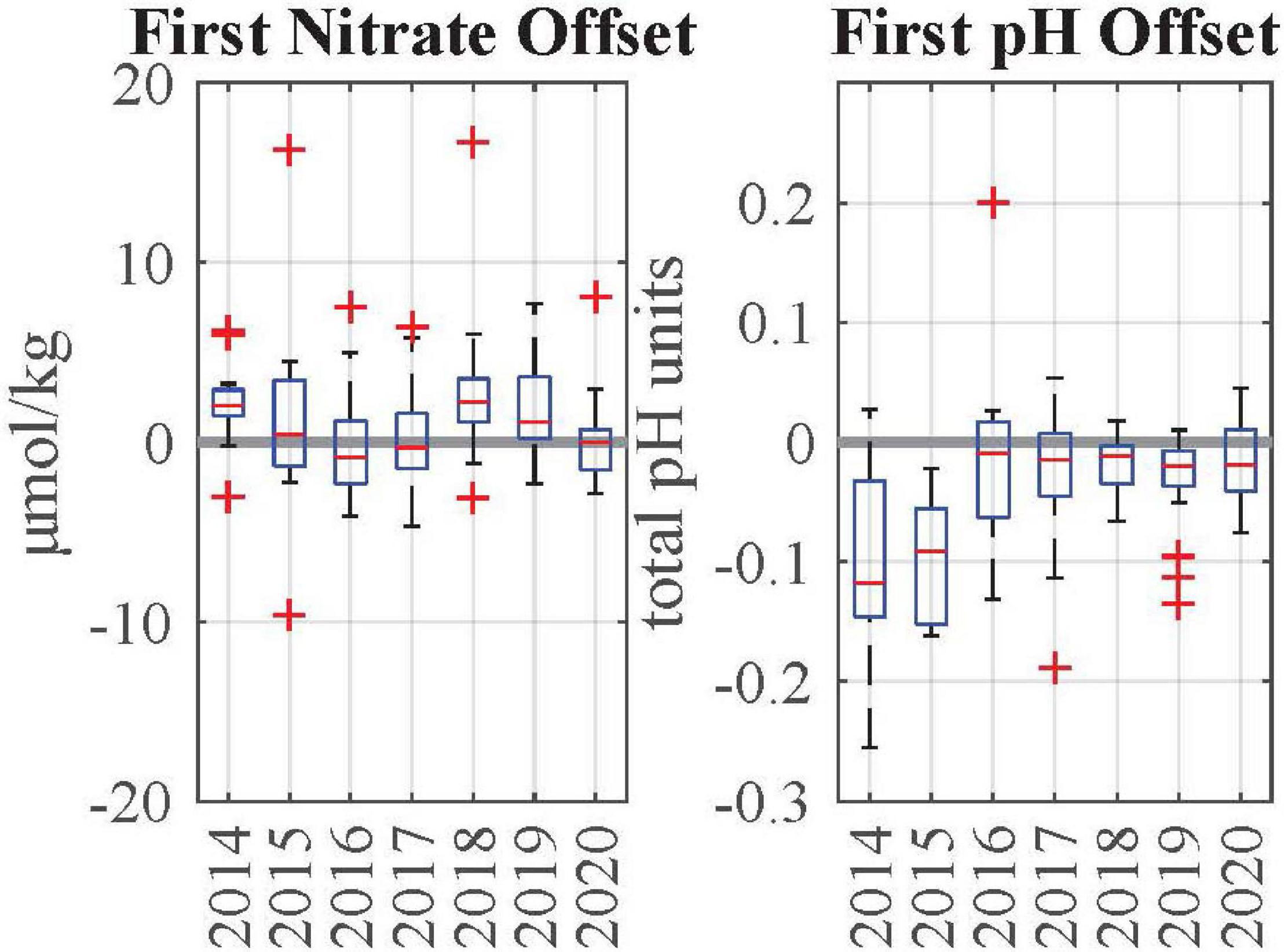
Figure 11. Boxplot summaries of first nitrate (left) and first pH (right) offsets, grouped by deployment year. Red lines represent the median, box boundaries represent the interquartile range (Q3–Q1), whiskers are the outer range of data, excluding outliers (red +) which are defined as data points that are larger than Q3 + 1.5 × (Q3 – Q1) or smaller than Q1 – 1.5 × (Q3 – Q1).

Validating SOCCOM Nitrate and pH Adjustments

In this section, we discuss a system for validating our calibration methods. This involves comparison of post-corrected float data to data from both high-quality shipboard bottle casts taken alongside each SOCCOM float at the time of deployment, and nearby stations within the GLODAPv2 dataset (Olsen et al., 2020). While shipboard data can also be useful for assessing initial offsets along a profile, it is not essential to float calibration and is almost always reserved as an independent validation of the employed correction methods.

The Use of Shipboard Bottle Data

With the exception of oxygen calibration on Navis floats, the methods described in the previous sections for adjusting chemical data from a float do not depend on the existence of shipboard reference data collected alongside a float’s deployment. This is advantageous in that any shipboard data taken at the time of deployment can be used to validate the applied in situ calibration methods. The SOCCOM program has required shipboard data collection alongside float deployment wherever possible to support the building of a robust validation dataset. However, because it is not essential to sensor QC, shipboard data collection may be reduced to select cruises in the future.

Comparisons of SOCCOM quality-controlled float data against shipboard data taken near the time of deployment are shown in Figures 12, 13. All float data have been interpolated onto the pressure axis of the hydrocast data. A portion of the error in the differences can be attributed to spatial and temporal changes in hydrography between the float profile and bottle samples. Float deployments typically occur as the ship begins heading away from a sampling station after the CTD rosette cast has been performed. This is done to reduce the chances of the ship running into the float. An additional lag time exists between deployment and when the float completes its first profile. Float-to-bottle matchups in the SOCCOM array are on average 23 h and 8 km apart in time and space because of this. Nonetheless, the float to bottle matchups show very good agreement. The slope of the Model II regression for each parameter is indistinguishable from the 1:1 line. The median bottle-minus-float difference for adjusted oxygen, nitrate, and pH data are 0.35 ± 6.8 μmol kg^–1, −0.12 ± 0.99 μmol kg^–1, and 0.002 ± 0.015 (1 SD) total pH units, respectively. If half of the SD is due to ocean variability between the time of bottle sampling and the float profile, then the float data would have uncertainties (1 SD) of about 3 μmol kg^–1, 0.5 μmol kg^–1, and 0.007 total pH, respectively. These values are very close to the accuracies reported in Johnson et al. (2017). Oxygen shows the largest improvement; this may partially be attributed to the implementation of the optode drift correction which was not yet accounted for at the time of the Johnson et al. (2017) publication.

FIGURE 12

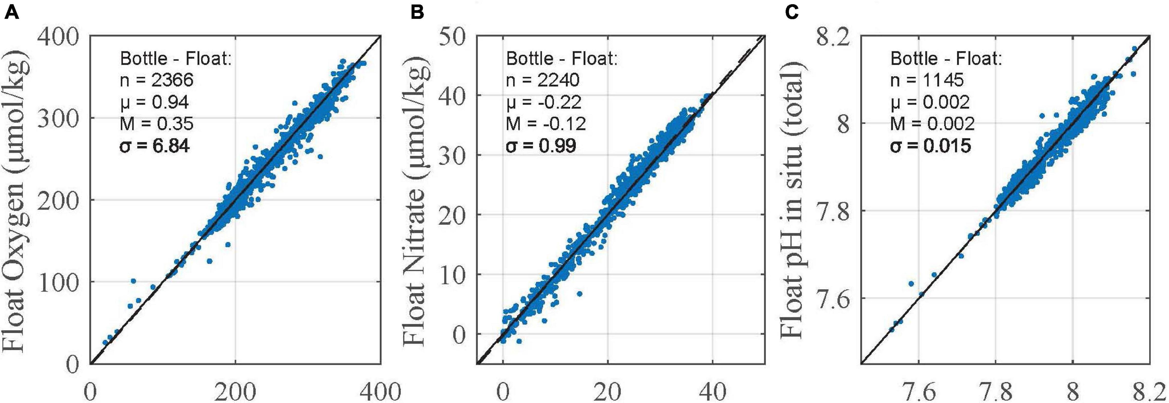
Figure 12. Scatterplots of adjusted float oxygen (A), nitrate (B), and pH (C) data versus shipboard bottle data (all depths). The solid and dashed lines represent the 1:1 and Model II least squares fit, respectively. Bottle-minus-float statistics [number of observations (n), mean (μ), median (M), and standard deviation (σ)] are included in the plots.

FIGURE 13

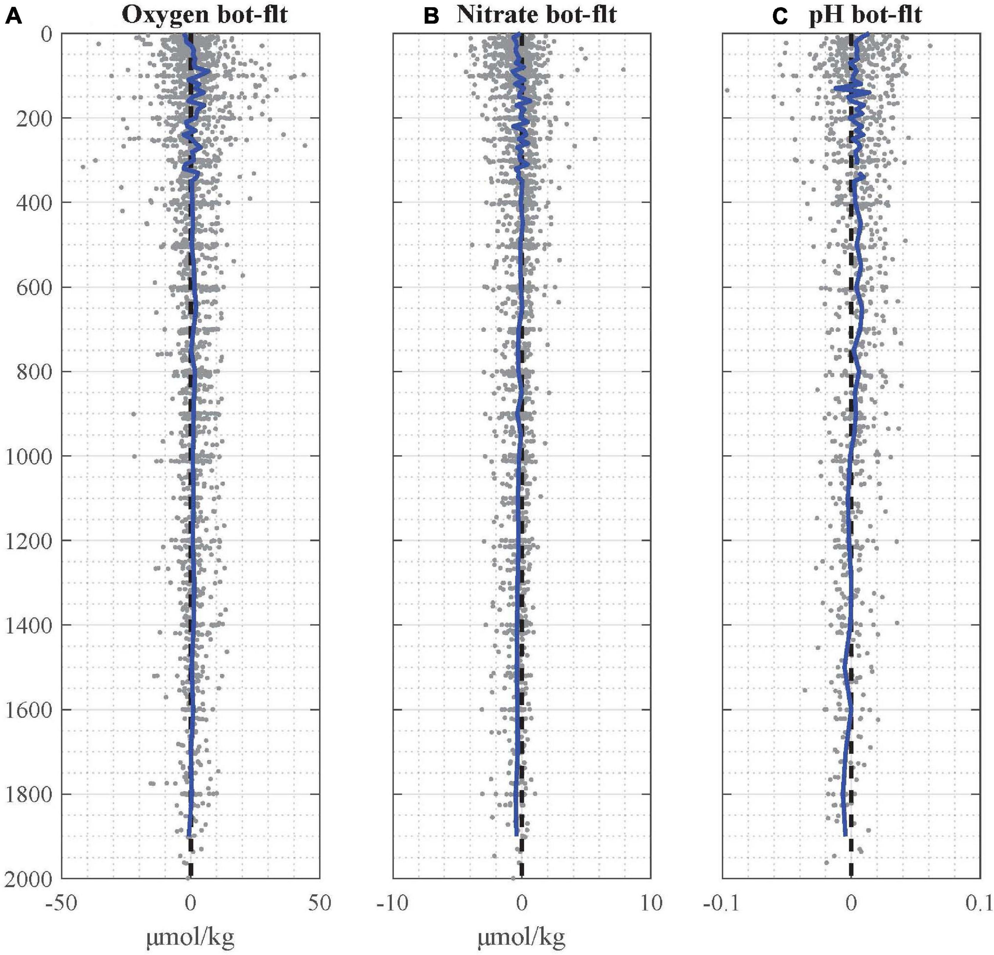
Figure 13. Scatterplots of bottle minus float matchups for adjusted (A) oxygen, (B) nitrate, and (C) pH data, plotted in depth space. Blue lines represent the mean of data within depth bins.

Additionally, an independent triple collocation analysis by Mignot et al. (2019) of quality controlled BGC-Argo float data in the Mediterranean Sea shows similar results, stating accuracies for oxygen and nitrate data of 2.9(5.1) and 0.46(0.25) μmol kg^–1, respectively [additive bias (rmse)]. Note that the triple collocation analysis involved float, model, and shipboard data, with the assumption that the shipboard data was perfectly calibrated (as described in the Mignot et al., 2019 supplemental). Maximum depths reached by floats in the Mignot et al. (2019) analysis was 1000 m, as opposed to 2000 m on SOCCOM floats. The upper water column, therefore, made up a larger relative proportion of their float-to-bottle dataset; spatio-temporal mismatch due to greater oceanic variability at these depths likely accounts for the slightly larger biases observed.

Float-to-bottle matchups in pressure space provide a validation of the assumption that sensor offsets are constant with depth (Johnson et al., 2013, 2016, 2017). Figure 13 shows the bottle-minus-float differences for all oxygen, pH, and nitrate matchups, plotted against pressure. The blue lines represent binned averages. There are no large trends in the oxygen or nitrate values with depth, confirming the assumptions in our calibration method. It is also apparent that the slow response of the oxygen sensor (Bittig et al., 2014) does not cause excessive offsets in the oxycline of the Southern Ocean, although this issue may be more serious in regions with steeper oxygen gradients. For pH, the pressure-binned distribution of mean differences show a negative bias of 5 millipH at depth. This bias changes sign toward the surface. Johnson et al. (2016) show a similar trend in comparison to discrete data (figure 6 in their publication, although note that the trend is reversed as their plot represents float-minus-discrete) which they attribute to an incomplete understanding of carbonate-system thermodynamics at high pressures. While the magnitude of this bias is within the limits of stated uncertainty in the pH correction method (see section “Nitrate and pH Adjustments Applied to SOCCOM Float Data”), the depth-dependent nature of the pH bias, as evident in the data, should be researched further.

Comparisons to GLODAPv2

As described in the previous section, SOCCOM data quality validation is performed primarily in reference to shipboard hydrographic data taken at the time of deployment. This method of validation is limited in scope to the initial profile returned from each float. Since in situ drift is often observed in nitrate and pH (and to a lesser degree, oxygen) sensors onboard SOCCOM floats, a logical question is whether or not the quality of the applied adjustments remains stable throughout the duration of a float’s life. For nitrate and pH, degradation in the quality of the adjustment over time could come from a few specific sources. Possible examples include a reduction in accuracy in one of the input parameters to the reference models (namely, temperature, salinity, or oxygen), or a reduction in the accuracy of the reference algorithm itself due to gradual changes in deep ocean conditions that challenge the validity of the empirical relationships over long time scales. The first possibility poses less of a threat, as temperature and salinity data on Argo floats are quite stable and require minimal adjustment. And, although drift is observed in some oxygen optodes onboard SOCCOM floats (see section “Drift in Optode Gain”), comparison to a stable atmospheric reference provides a robust means for correction. And, ensuring the validity of reference algorithms over time will require periodic updates to the model derivations in years to come. Other possible causes for degradation in data adjustment quality through time are potential changes in the pressure or temperature coefficients of the sensor. If such changes in calibration occurred, then corrections derived at depth as the sensor aged would not be accurate near the surface.

The impacts from the issues described in the preceding paragraph can be assessed for the current SOCCOM dataset through an independent comparison of SOCCOM quality-controlled data at different stages of a float’s life with hydrographic data from nearby stations in the GLODAPv2 dataset (Olsen et al., 2020). Figure 14 shows histograms of GLODAPv2 minus float data for oxygen, nitrate, and pH crossovers within 20 km distance of GLODAPv2 station data with no temporal restrictions. Because we chose to not constrain the matchup data temporally (doing so greatly reduces the number of matchups), only data below 300 dbar were used to minimize discrepancies due to seasonal variability in the upper water column. These matchup criteria are consistent with validation analysis performed in Johnson et al. (2017). The upper panels in the figure include comparisons from floats between 6 months and 2 years of age, and the lower panel includes data from floats greater than 2 years of age. A 3.59 μmol kg^–1 and 0.027 pH bias between float and GLODAPv2 data can be observed for oxygen and pH data, respectively for the young (6 months < age < 2 years) floats. Similar biases are observed for the old (age > 2 years) floats (3.82 μmol kg^–1 and 0.020 for oxygen and pH, respectively). If the quality of the adjusted float data were degrading over time, we would expect the biases to increase with comparisons using the older cohort of float data. The consistency of the biases for young and old floats are thus more likely a result of temporal differences between mean GLODAPv2 data used in the analysis and the corrected SOCCOM dataset. The mean age difference between the two datasets is 18.6 years. Both the oxygen and pH biases increase linearly as the age difference between the GLODAPv2 station time and the profiling float measurement time increases (Johnson et al., 2017; Swart et al., 2018). The observed rate of change in the pH bias across this time frame (0.001 pH year) is consistent with expected and observed rates of ocean pH decrease (Ríos et al., 2015; Williams et al., 2018) due to increasing atmospheric CO₂, which creates ocean acidification. A linear change in the oxygen bias over nearly two decades (0.2 μmol kg year) with Southern Ocean oxygen decreasing by 4 μmol kg is consistent with reported rates of oxygen change in the Southern Ocean that are based on shipboard data (Helm et al., 2011). These consistent rates of change lend support to our hypothesis that the biases for oxygen and pH seen in Figure 14 are the result of dynamic ocean change in the Southern Ocean in response to global climatic shifts (Bronselaer et al., 2020) and not due to instrument biases. This provides strong evidence that the QC methods continue to be accurate over the lifetime of the float.

FIGURE 14

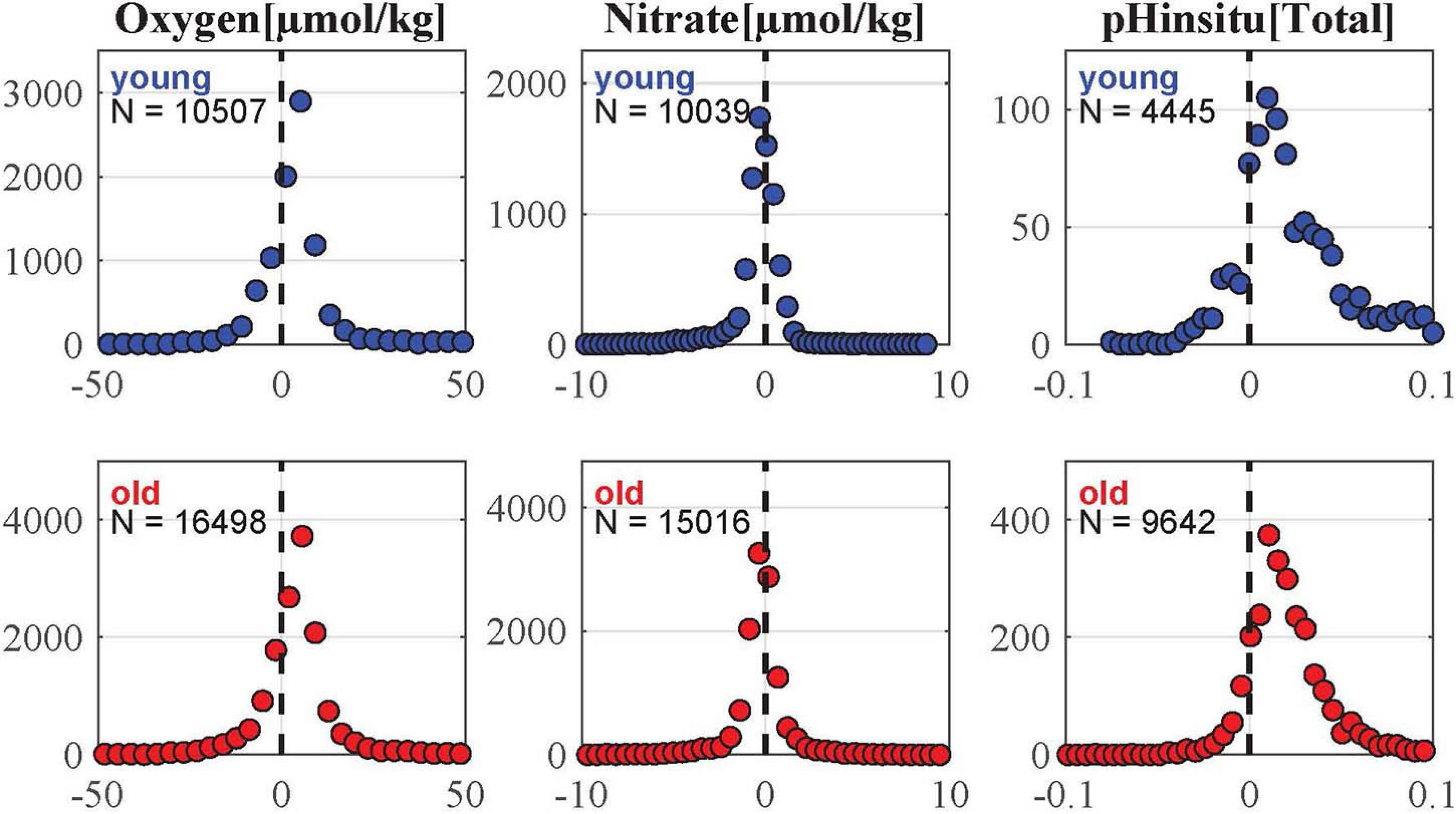
Figure 14. Histograms of GLODAPv2 minus quality-controlled oxygen (left), nitrate (center), and pH (right) float data. Upper panels include data from floats between 6 months and 2 years of age; lower panels include data from floats older than 2 years of age. Matchups were restricted to data that was within 20 km of GLODAPv2 reference stations.

Discussion

In this article, we presented a coherent framework for applying delayed-mode adjustment procedures to oxygen, nitrate, and pH data from SOCCOM biogeochemical profiling floats. The software presented, SAGE (SOCCOM Assessment and Graphical Evaluation) and SAGE-O₂, provide a robust way to visualize and assess the quality of these data. These software are open source and available through GitHub.¹ The tools are intended to be used periodically throughout a float’s life to reexamine sensor performance in delayed-mode. Adjustments derived using the software can then be applied to existing data and propagated forward in real-time until the next delayed-mode assessment is completed. A notable aspect of the procedure is in the relationship between the oxygen adjustment and that of nitrate and pH. The collective use of both SAGE-O₂ and SAGE offers a clear pathway to adjusted data for oxygen optodes, nitrate, and pH sensors, all of which commonly coexist on biogeochemical profiling float platforms.

The successful expansion of the BGC-Argo program on a global scale, as described by Roemmich et al. (2019), will partially depend on the implementation of standardized data adjustment methods across float platforms. The methods and software tools presented here have already been adopted for use by other Argo data centers and are helping to increase the level of high-quality biogeochemical profiling float data available to users around the world. Although these software were developed specifically for Ocean Data View – compatible ascii files used in the SOCCOM program (which also contain derived carbon parameters not found in Argo data files), data adjustments derived within the software can easily be integrated into Argo NetCDF data processing pathways. Structuring the tools in this way has allowed for flexibility in adaptation across data centers. Additionally, this flexibility means that applications are not limited to Argo float data. The SAGE tools have the potential for use in post-deployment calibration of nitrate and pH data from other platforms such as gliders as well (Takeshita et al., 2020). As Bushinsky et al. (2019b) describe, sustaining multiple types of observational platforms in the ocean can increase our ability to resolve key processes at different spatial and temporal scales and in regions particularly susceptible to the effects of global change such as coral reef habitats and coastal upwelling zones. Ensuring that biogeochemical data are comparable across platforms is therefore essential.

Furthermore, along with performing repeated, standardized QC procedures it is important to run validation analysis, as described in section “Validating SOCCOM Nitrate and pH Adjustments” with regularity. This provides a metric for tracking improvements to sensor accuracy over time and testing the effects of processing upgrades or changes in QC methodology on the quality of the dataset. While data from biogeochemical sensors onboard profiling floats are revolutionizing capabilities in global ocean carbon research and modeling (Ford, 2021), the operational limitations of the sensors and the measurements they provide cannot be overlooked. It is our hope that the calibration methods applied within the SOCCOM program, as outlined above, will serve as a global model for profiling float QC, but also that the validation that follows will help to constrain the scientific questions that can be asked and provide inspiration for future research in both chemical sensor development and QC.

Data Availability Statement

The datasets presented in this study can be found in online repositories. The names of the repository/repositories and accession number(s) can be found below: the comparison in section “Computation of Nitrate and pH Adjustments Using Automated Change-Point Detection” was done using SOCCOM data archives https://doi.org/10.6075/J0QJ7FJP and https://doi.org/10.6075/J01G0JKT. Float data used for analysis in all other sections can be found at https://doi.org/10.6075/J0B27ST5. Raw msg files returned from SOCCOM floats are also freely available at ftp://ftp.mbari.org/pub/SOCCOM/RawFloatData/. Shipboard data used in validation of SOCCOM float data are available through CCHDO (https://cchdo.ucsd.edu/search?q=soccom). World Ocean Atlas data used in this study can be found at https://www.ncei.noaa.gov/data/oceans/woa/WOA18/. GLODAPv2 data used in this study can be found at https://www.glodap.info/index.php/merged-and-adjusted-data-product/. NCEP Reanalysis data was provided by the NOAA/OAR/ESRL PSL, Boulder, CO, United States, from their website at https://psl.noaa.gov/.

Author Contributions

TM, JP, and KJ contributed to the development of the methodology, the validation presented, and the manuscript revision. TM and JP built the described software packages. TM prepared the initial manuscript. All authors contributed to the article and approved the submitted version.

Funding

All float data were collected and made freely available by the Southern Ocean Carbon and Climate Observations and Modeling (SOCCOM) project funded by the National Science Foundation, Division of Polar Programs (NSF PLR-1425989, with extension NSF OPP-1936222), supplemented by NASA, and by the International Argo Program and the NOAA programs that contribute to it. The Argo Program was part of the Global Ocean Observing System (https://doi.org/10.17882/42182, https://www.ocean-ops.org/board?t=argo). Additionally, all data analysis and supporting work performed at the Monterey Bay Aquarium Research Institute was supported in part by the David and Lucile Packard Foundation.

Conflict of Interest

The nitrate and pH sensors used in BGC-Argo were developed in KJ’s laboratory at the Monterey Bay Aquarium Research Institute, and the institution receives royalty payments from commercial licenses. KJ has recused himself from receiving any compensation from these licenses related to BGC-Argo.

The remaining authors declare that the research was conducted in the absence of any commercial or financial relationships that could be construed as a potential conflict of interest.

Publisher’s Note

All claims expressed in this article are solely those of the authors and do not necessarily represent those of their affiliated organizations, or those of the publisher, the editors and the reviewers. Any product that may be evaluated in this article, or claim that may be made by its manufacturer, is not guaranteed or endorsed by the publisher.

Acknowledgments

This work was made possible by the Southern Ocean Carbon and Climate Observations and Modeling (SOCCOM) project. The authors would like to thank all people who contributed to the production, calibration, and assembly of all sensors and floats used within SOCCOM, as well as all personnel involved in their transport and deployment at sea. The authors gratefully acknowledge contributions provided by Yui Takeshita and Annie Wong during the initial preparation of the manuscript. The authors would also like to thank MBARI 2018 summer intern, Tatjana Ellis, for her contributions to the testing of automated change-point-detection within the SAGE GUI framework. Special thanks to the two reviewers whose detailed comments have significantly improved the overall quality of the manuscript. MATLAB code for the SAGE and SAGE-O₂ software tools, including an operations manual for SAGE-O₂, is freely available at https://github.com/SOCCOM-BGCArgo/ARGO_PROCESSING/ (DOI: 10.5281/zenodo.5023965). Additionally, the MBARI code base used for generating Argo NetCDF B-files is also freely available at https://github.com/SOCCOM-BGCArgo/MBARI_ArgoBfile_generation. All code is subject to change. A preprint of this manuscript is available on the Earth and Space Science Open Archive (ESSOAr), (Maurer et al., 2021).

Footnotes

1. ^ https://github.com/SOCCOM-BGCArgo/ARGO_PROCESSING

References

Aanderaa Instruments (2017). TD269 Operating Manual, Oxygen Optode 4330, 4831, 4835, Seventh Edn. Bergen: Aanderaa Instruments.

Google Scholar

Bittig, H. C., Fiedler, B., Scholz, R., Krahmann, G., and Körtzinger, A. (2014). Time response of oxygen optodes on profiling platforms and its dependence on flow speed and temperature. Limnol. Oceanogr. Methods 12, 617–636. doi: 10.4319/lom.2014.12.617

CrossRef Full Text | Google Scholar

Bittig, H. C., and Körtzinger, A. (2015). Tackling oxygen optode drift: near-surface and in-air oxygen optode measurements on a float provide an accurate in situ reference. J. Atmos. Oceanic Technol. 32, 1536–1543. doi: 10.1175/JTECH-D-14-00162.1

CrossRef Full Text | Google Scholar

Bittig, H. C., and Körtzinger, A. (2017). Technical note: update on response times, in-air measurements, and in situ drift for oxygen optodes on profiling platforms. Ocean Sci. 13, 1–11. doi: 10.5194/os-13-1-2017

CrossRef Full Text | Google Scholar

Bittig, H. C., Körtzinger, A., Neill, C., van Ooijen, E., Plant, J. N., Hahn, J., et al. (2018a). Oxygen optode sensors: principle, characterization, calibration and application in the ocean. Front. Mar. Sci. 4:429. doi: 10.3389/fmars.2017.00429

CrossRef Full Text | Google Scholar

Bittig, H. C., Maurer, T. L., Plant, J. N., Schmechtig, C., Wong, A. P. S., Claustre, H., et al. (2019). A BGC-Argo guide: planning, deployment, data handling and usage. Front. Mar. Sci. 6:502. doi: 10.3389/fmars.2019.00502

CrossRef Full Text | Google Scholar

Bittig, H. C., Steinhoff, T., Claustre, H., Fiedler, B., Williams, N. L., Sauzède, R., et al. (2018b). An alternative to static climatologies: robust estimation of open ocean CO2 variables and nutrient concentrations from T, S, and O2 data using bayesian neural networks. Front. Mar. Sci. 5:328. doi: 10.3389/fmars.2018.00328

CrossRef Full Text | Google Scholar

Bronselaer, B., Russell, J., Winton, M., Williams, N., Key, R., Dunne, J., et al. (2020). Importance of wind and meltwater for observed chemical and physical changes in the Southern Ocean. Nat. Geosci. 13, 35–42. doi: 10.1038/s41561-019-0502-8

CrossRef Full Text | Google Scholar

Bushinsky, S. M., Emerson, S. R., Riser, S. C., and Swift, D. D. (2016). Accurate oxygen measurements on modified Argo floats using in situ air calibrations. Limnol. Oceanogr. Methods 14, 491–505. doi: 10.1002/lom3.10107

CrossRef Full Text | Google Scholar

Bushinsky, S. M., Landschützer, P., Rödenbeck, C., Gray, A. R., Baker, D., Mazloff, M. R., et al. (2019a). Reassessing Southern Ocean air-sea CO2 flux estimates with the addition of biogeochemical float observations. Global Biogeochem. Cycles. 33, 1370–1388. doi: 10.1029/2019GB006176

PubMed Abstract | CrossRef Full Text | Google Scholar

Bushinsky, S. M., Takeshita, Y., and Williams, N. L. (2019b). Observing changes in ocean carbonate chemistry: our autonomous future. Curr. Climate Change Rep. 5, 207–220. doi: 10.1007/s40641-019-00129-8

PubMed Abstract | CrossRef Full Text | Google Scholar

Carter, B. R., Feely, R. A., Williams, N. L., Dickson, A. G., Fong, M. B., and Takeshita, Y. (2018). Updated methods for global locally interpolated estimation of alkalinity, pH, and nitrate. Limnol. Oceanogr. Methods 16, 119–131. doi: 10.1002/lom3.10232

CrossRef Full Text | Google Scholar

D’Asaro, E. A., and McNeil, C. (2013). Calibration and stability of oxygen sensors on autonomous floats. J. Atmos. Oceanic Technol. 30, 1896–1906. doi: 10.1175/jtech-d-12-00222.1

CrossRef Full Text | Google Scholar

Drucker, R., and Riser, S. C. (2016). In situ phase-domain calibration of oxygen Optodes on profiling floats. Methods Oceanogr. 17, 296–318. doi: 10.1016/j.mio.2016.09.007

CrossRef Full Text | Google Scholar

Fabozzi, F. J., Focardi, S. M., Rachev, S. T., and Arshanapalli, B. G. (2014). The Basics of Financial Econometrics: Tools, Concepts, and Asset Management Applications. Appendix E: Model Selection Criterion: AIC and BIC. Hoboken, NJ: Wiley and Sons, Inc.

Google Scholar

Ford, D. (2021). Assimilating synthetic Biogeochemical-Argo and ocean colour observations into a global ocean model to inform observing system design. Biogeosciences 18, 509–534. doi: 10.5194/bg-18-509-2021

CrossRef Full Text | Google Scholar

Gaillard, F., Autret, E., Thierry, V., Galaup, P., Coatanoan, C., and Loubrieu, T. (2009). Quality control of large Argo datasets. J. Atmos. Oceanic Technol. 26, 337–351. doi: 10.1175/2008jtecho552.1

CrossRef Full Text | Google Scholar

Gray, A., Johnson, K. S., Bushinsky, S. M., Riser, S. C., Russell, J. L., Talley, L. D., et al. (2018). Autonomous biogeochemical floats detect significant carbon dioxide outgassing in the high-latitude Southern Ocean. Geophys. Res. Lett. 45, 9049–9057. doi: 10.1029/2018GL078013

PubMed Abstract | CrossRef Full Text | Google Scholar

Guinehut, S., Coatanoan, C., Dhomps, A. L., Le Traon, P. Y., and Larnicol, G. (2009). On the use of satellite altimeter data in Argo quality control. J. Atmos. Oceanic Technol. 26, 395–402. doi: 10.1175/2008JTECHO648.1

CrossRef Full Text | Google Scholar

Helm, K. P., Bindoff, N. L., and Church, J. A. (2011). Observed decreases in oxygen content of the global ocean. Geophys. Res. Lett. 38:L23602. doi: 10.1029/2011GL049513

CrossRef Full Text | Google Scholar

Hood, E. M., Sabine, C. L., and Sloyan, B. M. (eds) (2010). The GO-SHIP Repeat Hydrography Manual: A Collection of Expert Reports and Guidelines. IOCCP Report Number 14, ICPO Publication Series Number 134. Available online at http://www.go-ship.org/HydroMan.html (accessed February 1, 2021).

Google Scholar

Johnson, K. S., and Coletti, L. J. (2002). In situ ultraviolet spectrophotometry for high resolution and long term monitoring of nitrate, bromide and bisulfide in the ocean. Deep Sea Res. 49, 1291–1305.

Google Scholar

Johnson, K. S., Coletti, L., Jannasch, H., Sakamoto, C., Swift, D., and Riser, S. (2013). Long-term nitrate measurements in the ocean using the in situ ultraviolet spectrophotometer: Sensor integration into the apex profiling float. J. Atmos. Oceanic Technol. 30, 1854–1866. doi: 10.1175/JTECH-D-12-00221.1

CrossRef Full Text | Google Scholar

Johnson, K. S., Jannasch, H. W., Coletti, L. J., Elrod, V. A., Martz, T. R., Takeshita, Y., et al. (2016). Deep-Sea DuraFET: a pressure tolerant pH sensor designed for global sensor networks. Anal. Chem. 88, 3249–3256. doi: 10.1021/acs.analchem.5b04653

PubMed Abstract | CrossRef Full Text | Google Scholar

Johnson, K. S., Pasqueron De Fommervault, O., Serra, R., D’Ortenzio, F., Schmechtig, C., Claustre, H., et al. (2018a). Processing Bio-Argo Nitrate Concentration at the DAC Level. Argo Data Management. Brest: Ifremer, doi: 10.13155/46121

CrossRef Full Text | Google Scholar

Johnson, K. S., Plant, J. N., Coletti, L. J., Jannasch, H. W., Sakamoto, C. M., Riser, S. C., et al. (2017). Biogeochemical sensor performance in the SOCCOm profiling float array. J. Geophys. Res. Oceans 122, 6416–6436. doi: 10.1002/2017JC012838

CrossRef Full Text | Google Scholar

Johnson, K. S., Plant, J. N., and Maurer, T. L. (2018b). Processing BGC-Argo pH Data at the DAC level. Argo Data Management. Brest: Ifremer, doi: 10.13155/57195

CrossRef Full Text | Google Scholar

Johnson, K. S., Plant, J. N., Riser, S. C., and Gilbert, D. (2015). Air oxygen calibration of oxygen optodes on a profiling float array. J. Atmos. Oceanic Technol. 32, 2160–2172. doi: 10.1175/jtech-d-15-0101.1

CrossRef Full Text | Google Scholar

Johnson, K. S., Riser, S. C., and Ravichandran, M. (2019). Oxygen variability controls denitrification in the Bay of Bengal oxygen minimum zone. Geophys. Res. Lett. 46, 804–811. doi: 10.1029/2018GL079881

CrossRef Full Text | Google Scholar

Kalnay, E. M., Kanamitsu, M., Kistler, R., Collins, W., Deaven, D., Gandin, L., et al. (1996). The NCEP/NCAR 40-year reanalysis project. Bull. Am. Meteorol. Soc. 77, 437–470.

Google Scholar

Kass, R. E., and Raferty, A. E. (1995). Bayes factors. J. Am. Stat. Assoc. 90, 773–795.

Google Scholar

Killick, R., Fearnhead, P., and Eckley, I. A. (2012). Optimal detection of changepoints with a linear computational cost. J. Am. Stat. Assoc. 107, 1590–1598. doi: 10.1080/01621459.2012.737745

CrossRef Full Text | Google Scholar

Klatt, O., Boebel, O., and Fahrbach, E. (2007). A profiling float’s sense of ice. J. Atmos. Oceanic Technol. 24, 1301–1308. doi: 10.1175/jtech2026.1

CrossRef Full Text | Google Scholar

Maurer, T. L., Plant, J. N., and Johnson, K. S. (2021). Delayed-mode quality control of oxygen, nitrate and pH data on SOCCOM biogeochemical profiling floats. ESSOAr [Preprint] doi: 10.1002/essoar.10506241.1

CrossRef Full Text | Google Scholar

Mignot, A., D’Ortenzio, F., Taillandier, V., Cossarini, G., and Salon, S. (2019). Quantifying observational errors in Biogeochemical-Argo oxygen, nitrate, and chlorophyll a concentrations. Geophys. Res. Lett. 46, 4330–4337. doi: 10.1029/2018GL080541

CrossRef Full Text | Google Scholar

Nicholson, D. P., and Feen, M. L. (2017). Air calibration of an oxygen optode on an underwater glider. Limnol. Oceanogr. Methods 15, 495–502. doi: 10.1002/lom3.10177

CrossRef Full Text | Google Scholar

Olsen, A., Lange, N., Key, R., Tanhua, T., Bittig, H., Kozyr, A., et al. (2020). GLODAPv2.2020 – the Second Update of GLODAPv2, Earth System Science Data Discussions. doi: 10.5194/essd-2020-165

CrossRef Full Text | Google Scholar

Owens, B. W., and Wong, A. P. S. (2009). An improved calibration method for the drift of the conductivity sensor on autonomous CTD profiling floats by θ-S climatology. Deep Sea Res. Part I Ocean Res. Papers 56, 450–457. doi: 10.1016/j.dsr.2008.09.008

CrossRef Full Text | Google Scholar

Ríos, A. F., Resplandy, L., García-Ibáñez, M. I., Fajar, N. M., Velo, A., Padin, X. A., et al. (2015). Decadal acidification in the water masses of the Atlantic Ocean. Proc. Natl. Acad. Sci. U.S.A. 112, 9950–9955. doi: 10.1073/pnas.1504613112

PubMed Abstract | CrossRef Full Text | Google Scholar

Riser, S. C., Swift, D., and Drucker, R. (2018). Profiling floats in SOCCOM: technical capabilities for studying the Southern Ocean. J. Geophys. Res. Oceans 123, 4055–4073. doi: 10.1002/2017JC013419

CrossRef Full Text | Google Scholar

Roemmich, D., Alford, M. H., Claustre, H., Johnson, K., King, B., Moum, J., et al. (2019). On the future of argo: a global, full-depth, multi-disciplinary array. Front. Mar. Sci. 6:439. doi: 10.3389/fmars.2019.00439

CrossRef Full Text | Google Scholar

Russell, J. L., Kamenkovich, I., Bitz, C., Ferrari, R., Gille, S. T., Goodman, P. J., et al. (2018). Metrics for the evaluation of the southern ocean in coupled climate models and earth system models. J. Geophys. Res. Oceans 123, 3120-3143. doi: 10.1002/2017JC013461

CrossRef Full Text | Google Scholar

Salstein, D. A., Ponte, R. M., and Cady-Pereira, K. (2008). Uncertainties in atmospheric surface pressure fields from global analyses. J. Geophys. Res. 113:D14107.

Google Scholar

Sauzède, R., Bittig, H. C., Claustre, H., Pasqueron de Fommervault, O., Gattuso, J.-P., Legendre, L., et al. (2017). Estimates of water-column nutrient concentrations and carbonate system parameters in the global ocean: a novel approach based on neural networks. Front. Mar. Sci. 4:128. doi: 10.3389/fmars.2017.00128

CrossRef Full Text | Google Scholar

Schmechtig, C., Herve, C., Antoine, P., and D’Ortenzio, F. (2018a). Bio-Argo Quality Control Manual for the Chlorophyll-A Concentration. doi: 10.13155/35385

CrossRef Full Text | Google Scholar

Schmechtig, C., Antoine, P., Hervé, C., D’Ortenzio, F., Dall’Olmo, G., and Emmanuel, B. (2018b). Processing bio-argo particle backscattering at the DAC level. Argo Data Manag. doi: 10.13155/39459

CrossRef Full Text | Google Scholar

Schwarz, G. (1978). Estimating the dimension of a model. Ann. Statist. 6, 461–464. doi: 10.1214/aos/1176344136

CrossRef Full Text | Google Scholar

Schmechtig, C., Organelli, E., Poteau, A., Claustre, H., and D’Ortenzio, F. (2017). Processing BGC-Argo CDOM Concentration at the DAC Level. Brest: Ifremer.

Google Scholar

Schmechtig, C., Poteau, A., Claustre, H., D’Ortenzio, F., and Boss, E. (2015). Processing Bio-Argo Chlorophyll-A Concentration at the DAC Level. Brest: Ifremer.

Google Scholar

Schmechtig, C., Thierry, V., and The Bio Argo Team. (2016). Argo Quality Control Manual for Biogeochemical Data. Bermuda: Bio-Argo group.

Google Scholar

Swart, S., Gille, S. T., Delille, B., Josey, S., Mazloff, M., Newman, L., et al. (2019). Constraining Southern Ocean Air-Sea-Ice fluxes through enhanced observations. Front. Mar. Sci. 6:421. doi: 10.3389/fmars.2019.00421

CrossRef Full Text | Google Scholar

Swart, S., Johnson, K. S., Mazloff, M. R., Meijers, A., Meredith, M. P., Newman, L., et al. (2018). The Southern Ocean, [in “State of the Climate in 2017”]. Bull. Amer. Meteor. Soc. 99, S185–S190. doi: 10.1175/2018BAMSStateoftheClimate.1

CrossRef Full Text | Google Scholar

Takeshita, Y., Jones, B. D., Johnson, K. S., Chavez, F. P., Rudnick, D. L., Blum, M., et al. (2020). Accurate pH and O2 measurements from Spray underwater gliders. J. Atmos. Oceanic Technol. 38, 181–195. doi: 10.1175/JTECH-D-20-0095.1

CrossRef Full Text | Google Scholar

Takeshita, Y., Martz, T. R., Johnson, K. S., Plant, J. N., Gilbert, D., Riser, S. C., et al. (2013). A climatology-based quality control procedure for profiling float oxygen data. J. Geophys. Res. Oceans 118, 5640–5650. doi: 10.1002/jgrc.20399

CrossRef Full Text | Google Scholar

Thierry, V., Bittig, H., Gilbert, D., Kobayashi, T., Kanako, S., and Schmid, C. (2018a). Processing Argo Oxygen Data at the DAC Level. Brest: Ifremer.

Google Scholar

Thierry, V., Bittig, H., and The Argo-Bgc Team. (2018b). Argo Quality Control Manual for Dissolved Oxygen Concentration. Brest: Ifremer.

Google Scholar

Verdy, A., and Mazloff, M. R. (2017). A data assimilating model for estimating Southern Ocean biogeochemistry. J. Geophys. Res. Oceans 122, 6968–6988. doi: 10.1002/2016JC012650

CrossRef Full Text | Google Scholar

Williams, N. L., Juranek, L. W., Feely, R. A., Russell, J. L., Johnson, K. S., and Hales, B. (2018). Assessment of the carbonate chemistry seasonal cycles in the Southern Ocean from persistent observational platforms. J. Geophys. Res. Oceans 123, 4833–4852. doi: 10.1029/2017JC012917

CrossRef Full Text | Google Scholar

Williams, N. L., Juranek, L. W., Johnson, K. S., Feely, R. A., Riser, S. C., Talley, L. D., et al. (2016). Empirical algorithms to estimate water column pH in the Southern Ocean. Geophys. Res. Lett. 43, 3415–3422. doi: 10.1002/2016GL068539

CrossRef Full Text | Google Scholar

Wong, A. P. S., Johnson, G. C., and Owens, W. B. (2003). Delayed-mode calibration of autonomous CTD profiling float salinity data by θ-S climatology. J. Atmospher. Oceanic Technol. 20, 308–318. doi: 10.1175/1520-0426(2003)020<0308:dmcoac>2.0.co;2

CrossRef Full Text | Google Scholar

Wong, A. P. S., Wijffels, S. E., Riser, S. C., Pouliquen, S., Hosoda, S., Roemmich, D., et al. (2020). Argo Data 1999–2019: two million temperature-salinity profiles and subsurface velocity observations from a global array of profiling floats. Front. Mar. Sci. 7:700. doi: 10.3389/fmars.2020.00700

CrossRef Full Text | Google Scholar