 Zhipeng Zhang
 Hongzhou Xu
 Philip A. Vetter
 Qiang Xie1,3
94% of researchers rate our articles as excellent or good
Learn more about the work of our research integrity team to safeguard the quality of each article we publish.
Find out more
ORIGINAL RESEARCH article
Front. Mar. Sci., 22 July 2021
Sec. Physical Oceanography
Volume 8 - 2021 | https://doi.org/10.3389/fmars.2021.681993
High-frequency motions in the southeastern South China Sea (SCS) have rarely been investigated due to sparse field observations. The vertical distribution and temporal variation of internal tides (ITs) and near-inertial waves (NIWs) near the Nansha area in the southeastern SCS were studied using a mooring current dataset from December 2018 to June 2019 in this study. Results showed that ITs were mainly dominated by O1, K1, and M2. Tidal energy analysis indicates that the diurnal ITs were the most energetic components, followed by the semidiurnal ITs. Modal decomposition reveals that diurnal ITs were dominated by mode-3, rather than mode-1, as reported by previous studies. The horizontal kinetic energy (HKE) of diurnal ITs fluctuated within a limited range, almost unaffected by the background field. However, the HKE of semidiurnal ITs was dominated by mode-1 and more affected by the background field, especially at the end of March. Most observations showed the phase of the NIWs propagating upward and the energy propagating downward. During the northeast monsoon period, the near-inertial energy had a large magnitude due to strong wind forcing. In addition, the near-inertial energy peaked from the middle of March to the beginning of April because of the input of NIWs from afar. Overall, near-inertial energy was found concentrated above a 500–600 m depth in the southeastern SCS.
Internal waves occur in stratified ocean with frequencies between the Coriolis frequency and the buoyancy frequency (Alford, 2003; Helfrich and Melville, 2006). Internal tides (ITs) and near-inertial waves (NIWs) are the most energetic components of internal waves; both play significant roles in oceanic mixing and circulation. ITs are generated when barotropic currents pass over abrupt topography (Garrett and Kunze, 2007; Xu et al., 2013). NIWs can be triggered by different mechanisms, such as non-linear interactions, surface wind forcing, geostrophic adjustment, and lee waves over ocean topography (Alford, 2003; van Aken et al., 2007; Xu et al., 2013; Alford et al., 2016). After the generation of ITs, high-mode components dissipate locally, while low-mode components propagate a long distance and their energy can enhance ocean turbulent mixing via many dissipation mechanisms (Alford and Zhao, 2007; Xie et al., 2008, Xie et al., 2011; Shang et al., 2015).
The ITs and NIWs in the South China Sea (SCS) have been observed frequently and have become the focus of extensive research. The strongest ITs throughout the world are generated in the Luzon Strait and then propagate into the northern SCS and the Pacific (Duda et al., 2004; Duda and Rainville, 2008; Liu et al., 2019). Jan et al. (2007), considering a three-dimensional non-linear mode, found that the more complex topography in the southern SCS can trigger local ITs with different wavelengths. Monsoons and extreme weather events can trigger NIWs locally in the SCS. Based on four sets of mooring data, Guan (2014) considered that due to the influence of monsoons, the near-inertial energy in the upper layer in the northern SCS in winter was 30–106% stronger than in summer, while in the deep layer in winter, it was 18–88% stronger than in summer.
Xie et al. (2010) found that tidal super-harmonic and sub-harmonic motions in the northern SCS mainly arose from parametric sub-harmonic instability (PSI). PSI is a non-linear weak interaction that can cause energy conversion among NIWs and waves with other frequencies. Qiu et al. (2019) implied that in summer and autumn in the northern SCS the stratification would increase. Guo et al. (2012) pointed out that the strong stratification is favorable for preserving the internal tidal energy and maintaining the IT waveform. Xu et al. (2013) showed that semidiurnal ITs with a multimodal structure can be more affected by a background current field and stratification structure than diurnal ITs. Moreover, NIWs observed in the northern SCS are considered to be caused by wind forcing, geostrophic adjustment, and the reflection of downward propagating NIWs from seafloor or the thermocline.
Shang et al. (2015) found that diurnal ITs in the west Nansha area were dominated by mode-1, while semidiurnal ITs had a more intermittent and multimodal structure. In addition, there was a semi-annual cycle in the diurnal barotropic currents due to the interference of K1 and P1 in the Nansha area. Liu et al. (2016) revealed that the energy of coherent and incoherent ITs in the western Nansha area accounted for 64% and 36% of internal tidal energy, respectively. Through calculation of a forcing term, the southeast and northeast of the Nansha area are considered to be the two main generation regions of ITs in the south of the SCS. Liang et al. (2016) indicated that mode-1 and mode-3 diurnal ITs contained most of the diurnal IT energy on the slope northwest of the SCS, and the semidiurnal ITs were dominated by mode-1.
Mesoscale eddies are considered to have potential impacts on mixing in the deep ocean. The existence of warm eddies is more conducive to propagation of near-inertial energy through the mixing layer toward the deep ocean, while cold eddies will hinder propagation (Benjamin and Shay, 2010). Liu et al. (2019) suggested that low-mode diurnal energy can be transferred to higher modes by near-critical reflection on the slope. Considerable energy still existed in semidiurnal ITs on the shelf in the northeastern SCS. Gao et al. (2019) found that moderate or weak wind curl favors the downward propagation of NIWs. In contrast, although strong cyclones can bring more energy, the energy will be limited to the upper layer. In addition, a large negative or positive sea level anomaly (SLA), which can accumulate large shear in the pycnocline, is also not suitable for NIWs to propagate deeper.
The southeastern SCS is studded with many islands and sea hills. However, the characteristics of the ITs and NIWs in this area are still unclear because of scarce in-situ observation. To reveal the characteristics of internal waves in this area, a mooring with an acoustic Doppler current profiler (ADCP) was deployed near the eastern Nansha area of the southeastern SCS and the observed data were used to analyze and record the structure and variation in this area.
Using an ADCP, the ocean current velocity at 9.66°N, 115.33°E (Figure 1) from December 7, 2018, to June 24, 2019, was recorded. Based on this, we set out to study the internal waves in the eastern Nansha area. The whole observation time included both the monsoon onset period and the monsoon transition period. Our mooring station was set on a slope surrounded by complex topography, with a water depth of 1,350 m. The 75-kHz up-looking ADCP was positioned at 750 m, covering the depth from 157 to 741 m with a vertical interval of 8 m, and measured the currents every 30 min. The surface layer of ADCP was neglected due to large fluctuation. In order to facilitate the subsequent processing of the data, the ADCP velocity profile data were linearly interpolated vertically to 5-m intervals from 175 to 740 m.
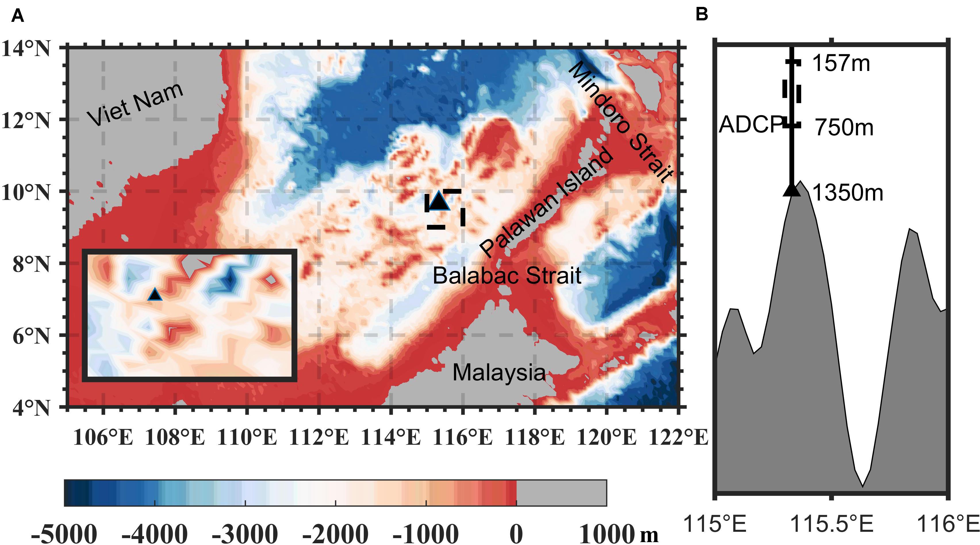
Figure 1. Topography of the south of the South China Sea (A), using the topographic data obtained from ETOPO1 (https://www.ngdc.noaa.gov/mgg/global/global.html). The black triangle is the mooring station. Zonal topography and observing profile of the mooring station (B), where the water depth is 1,350 m. The 75 kHz up-looking ADCP was positioned at 750 m, measuring the velocity from 157 to 741 m.
The time series of the raw current velocity is displayed in Figure 2. It can be seen that the currents varied greatly with time and depth during the observation period. From December to January, the area was dominated by southeastward currents. Then, it changed into northeastward currents starting from January. During mid-April, the currents showed a two-layer structure: northwestward in the upper layer (165–300 m) and northeastward in the lower layer (300–740 m). Gradually, the currents transformed into northeastward in the upper layer and northwestward in the lower layer in May.
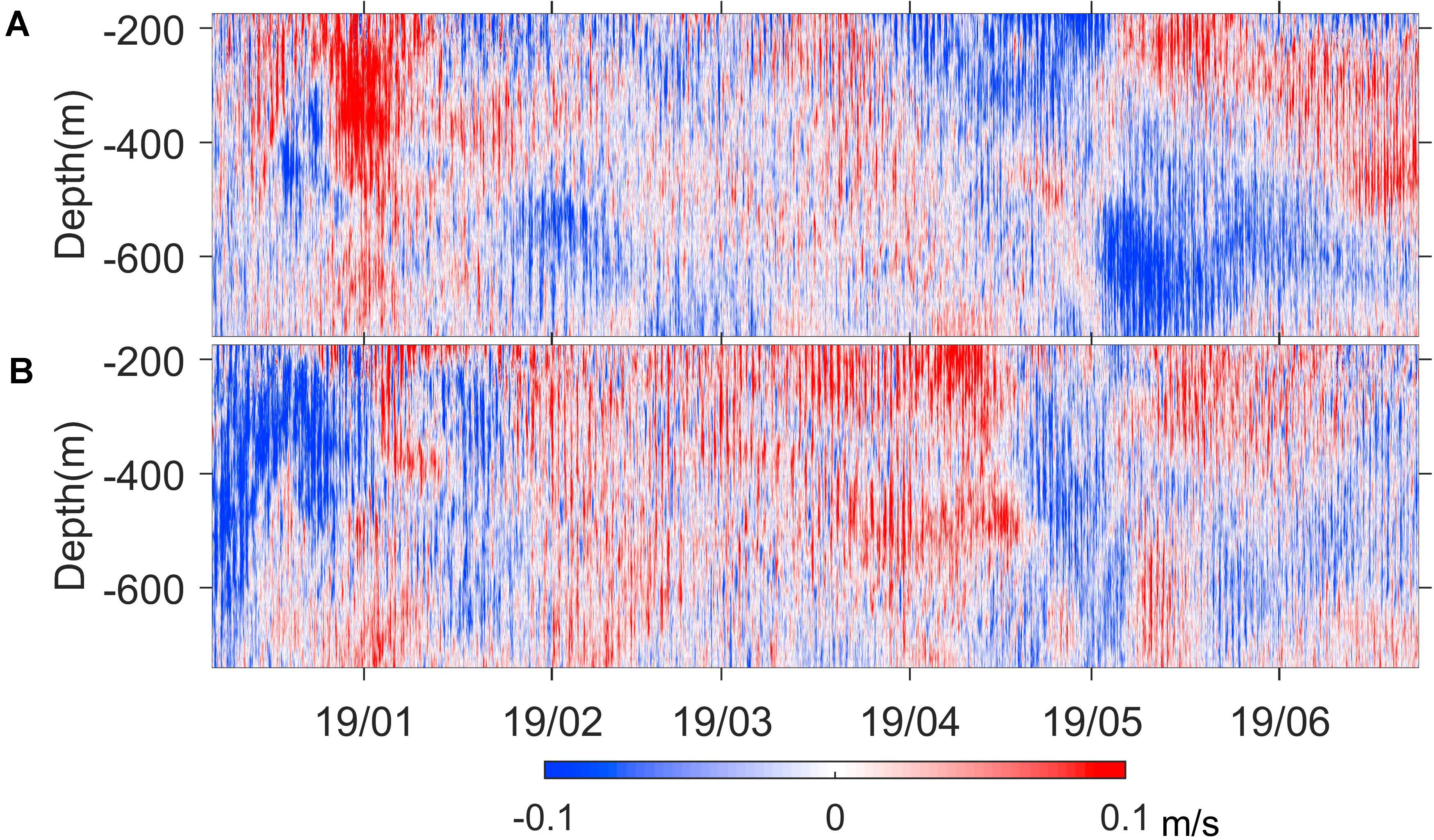
Figure 2. Time series of the meridional (A) and zonal (B) components of current velocity (m/s) at the mooring station.
To further study the generation and propagation mechanism of internal waves, we also used the following public datasets: monthly average thermohaline data with 0.25° × 0.25° resolution from the World Ocean Atlas 2018 (WOA18)1, hourly 10-m wind speed and wind stress curl data with 0.25° × 0.25° resolution from the European Center for Medium-Range Weather Forecasts (ECMWF)2, and daily SLA and geostrophic current data with 0.25° × 0.25° resolution from the Copernicus Marine Environment Monitoring Service (CMEMS)3. To document barotropic tides at the observation station, we used tidal mode data from the Oregon State Ocean Topography Experiment/Poseidon 7.2 (TPXO7.2, Egbert and Erofeeva, 2002) with 1/30° resolution in the China Seas.
Rotary spectra, which can be used for diagnosing the direction of the rotation of horizontal velocity with time or depth, are a kind of spectral analysis first proposed by Gonella (1972). The rotary spectra of time series are called rotary frequency spectra, while the rotary spectra of vertical space are named rotary wave number spectra. Its basic theory is as follows:
WKB-scaled velocity vector can be written in the complex form:
WKB-scaled velocity is computed by,
where N(z) is the profile of buoyancy frequency calculated by WOA18 salinity and temperature, and is the depth-average buoyancy frequency.
After Fourier transforms, uwt and vwt can be written as follows:
The equation of velocity is:
Clockwise spectrum is defined as:
Counterclockwise spectrum is defined as:
∗ denotes the conjugate complex number.
A fourth-order Butterworth band-pass filter was used to separate the diurnal, semidiurnal, and near-inertial components according to the rotary spectra. Accordingly, the cutoff frequencies that we chose were (0.85–1.1) cpd, (1.7–2.2) cpd, and (0.28–0.39) cpd, respectively. Harmonic analysis was performed on the time series of barotropic currents and baroclinic currents, respectively, in order to distinguish barotropic tides from ITs. The barotropic currents are considered to be the depth-averaged flows. The baroclinic currents are considered to be the raw currents minus the barotropic flows.
Vertically, internal waves can be regarded as the superposition of numerous waves of different wave number. They can be separated by modal decomposition via solving Sturm–Liouville eigenvalue problems:
The boundary conditions are,
where N2 is the square of buoyancy frequency calculated by WOA18 (World Ocean Atlas 2018), Cn is the eigenspeed (Gill, 1982), ρ0 is the density of water, using a constant value as ρ0 = 1024kg/m3 here, n is the mode number (n = 0 is defined to be the barotropic mode), Φ(z) is the vertical displacement, and Π(z) is the horizontal velocity.
The baroclinic velocity of each mode can be extracted by:
where is the time-varying magnitudes of each baroclinic mode, computed by least-square modal fitting at each time point, using the observed velocity profile.
It is the lack of mooring data at the surface and bottom layers that will render higher-mode fits unstable in the modal decomposition (Zhao et al., 2010; Shang et al., 2015). In addition, the results of analysis may not be applicable to the whole depth. In most cases, the ITs are dominated by low modes. Hence, we merely extracted the first three baroclinic modes and the barotropic mode. Based on Eqs. (11–13), modal structure and vertical distribution of the square buoyancy frequency were estimated at the observation station (Figure 3). In addition, the depth-integrated horizontal kinetic energy (HKE) can be calculated by,
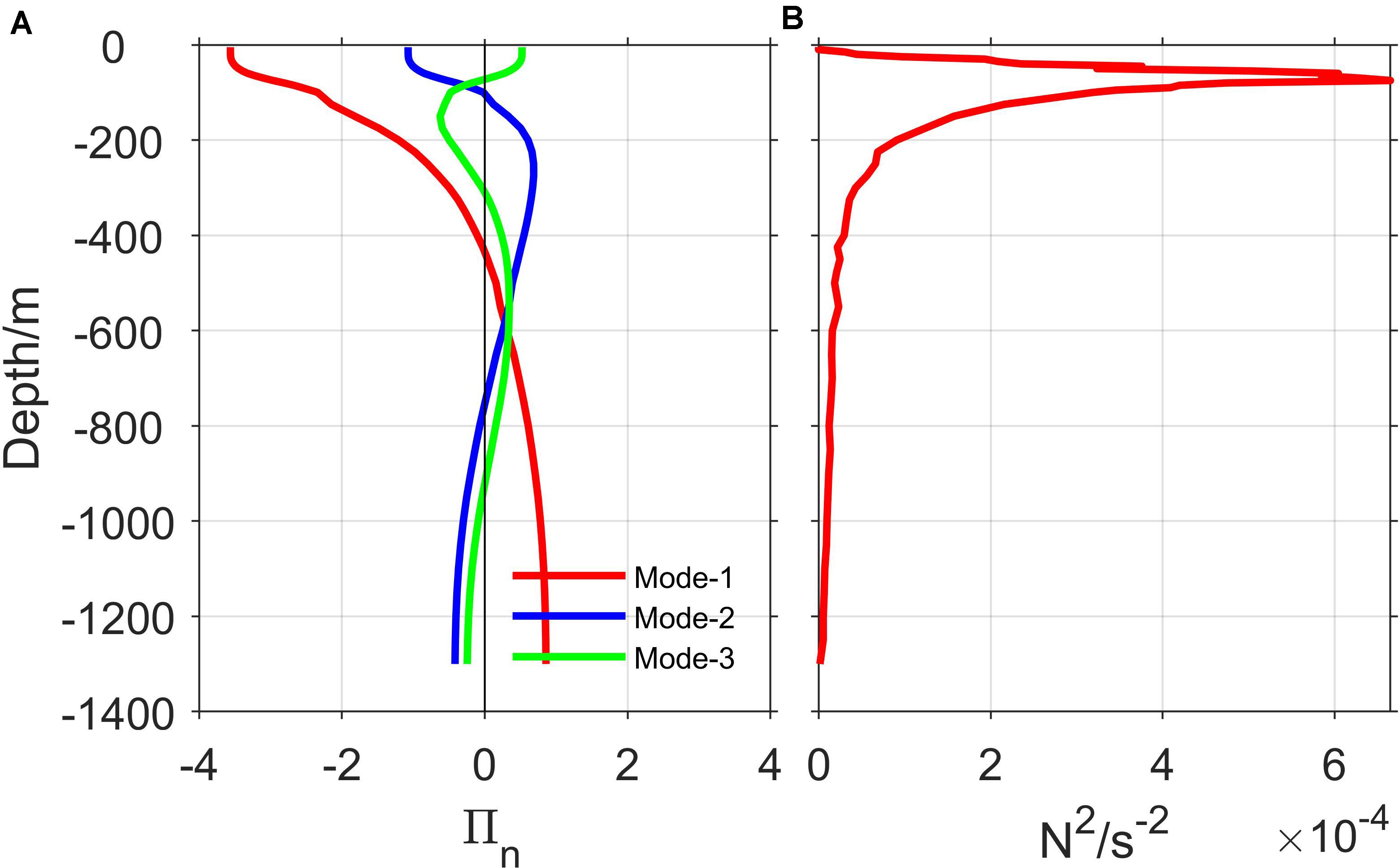
Figure 3. Modal structure (A) and the vertical distribution of the square Brunt-Vaisala (B) during the observation period at the mooring station, computed by WOA18. Horizontal labels mark the start of the month.
where the angle bracket is the internal wave cycle time average.
Figure 4 shows eight main components of observed (red) and TOXO7.2 predicted (blue) barotropic tidal ellipses at the mooring station. The major axis and minor axis of the ellipses indicate the maximum and minimum amplitudes of the tidal currents, while the inclination of the ellipse represents the phase. It can be seen that observed barotropic tidal currents are similar to that of TPXO7.2; both are mainly dominated by O1, K1, and M2 tides. However, a difference in phase between them is visible. This discrepancy may be caused by the absence of observed data at the surface and bottom layers. In addition, phases of eight major components show significant differences, in that the major axes of Q1, O1, P1, and N2 are oriented in the northeast–southwest direction, while K1, M2, S2, and K2 are oriented in the northwest–southeast direction.
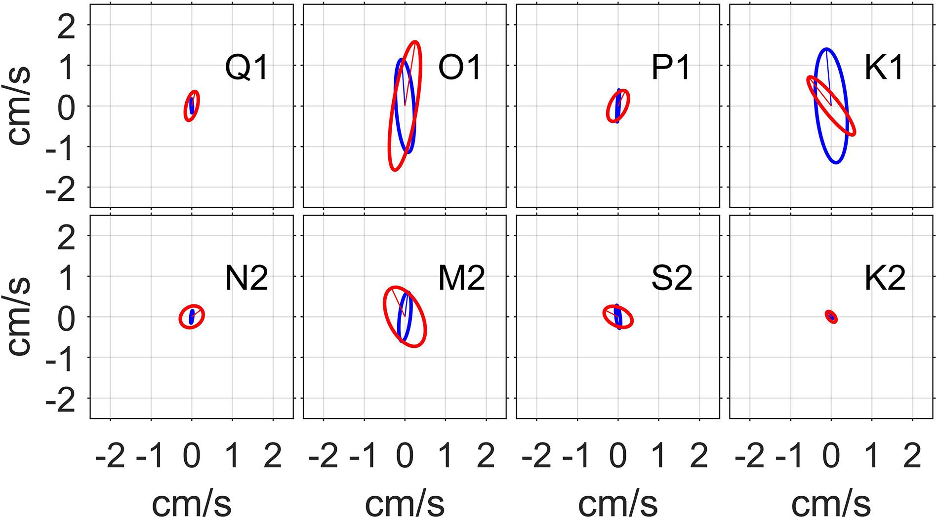
Figure 4. Observed barotropic tidal ellipses (red) and barotropic tidal ellipses predicted from TOXO7.2 (blue).
Since the ITs are not uniform in depth, harmonic analysis should be conducted for each depth, respectively. Figure 5 reveals the tidal ellipses of eight baroclinic components. The diurnal ITs are dominated by K1 and O1, the semidiurnal ITs by M2. Complex variations emerge in both diurnal and semidiurnal ITs vertically, implying that they might have vertical multimodal structures. In addition, the eight major baroclinic components show clockwise polarization significantly at most depths; this is in accordance with the polarization of freely propagating waves in the northern hemisphere (van Haren, 2005; Xie et al., 2010; Shang et al., 2015).
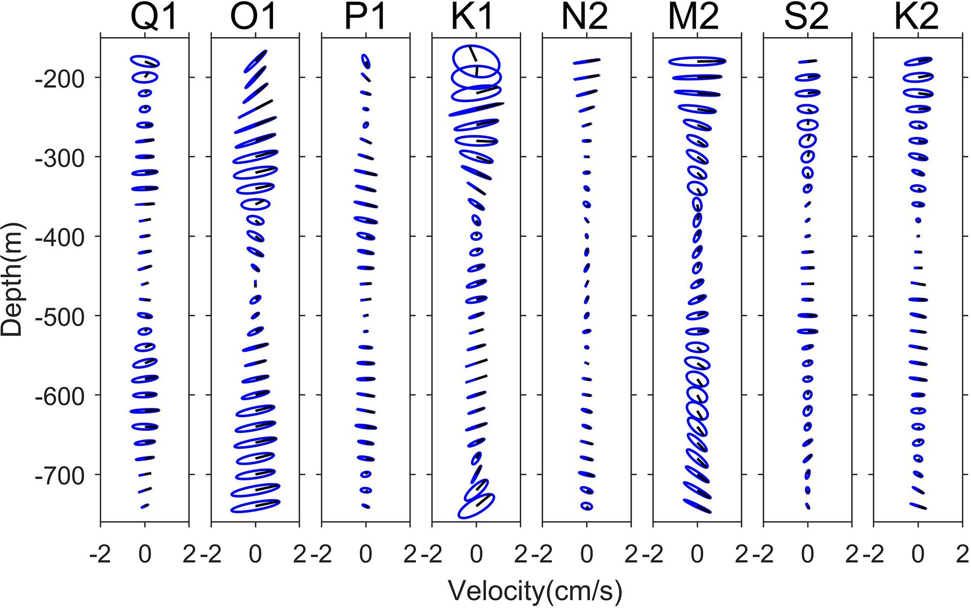
Figure 5. Vertical distribution of baroclinic tidal ellipses for eight main tide components.
The average rotary spectra from 175 to 740 m were calculated (Figure 6), wherein the clockwise spectra show significant peaks at the near-inertial, diurnal, and semidiurnal frequencies. Nevertheless, most of the counterclockwise component energy is concentrated on diurnal and semidiurnal components, with no peak shown at the near-inertial frequency. In addition, perceptible but not considerable peaks are evinced at frequencies of superposition of diurnal tides and NIWs (f+K1), due to non-linear interaction. Higher harmonics (M2+O1, M2+K1, M4, and M2+S2) are also found to have obvious peaks, possibly owing to advection and non-linear interaction among diurnal and semidiurnal tides. The bulk of the energy is focused on the clockwise component in the northern hemisphere, and the clockwise component energies of diurnal, semidiurnal, and near-inertial components are comparable, although the diurnal component is slightly larger. NIWs are almost entirely clockwise, which means most of the near-inertial energy is concentrated in the clockwise components. The previous studies in the northern SCS (Xu et al., 2013; Guan, 2014) showed that the energy of clockwise components at diurnal frequencies can be more than 10 times that of the counterclockwise components. However, we find that in the observation station the clockwise spectra at diurnal frequencies are close to the counterclockwise spectra at diurnal frequencies; the energy of the clockwise component at diurnal frequencies is only three times larger than that of the counterclockwise component at diurnal frequencies in the southeastern SCS. In the northern SCS, the larger amplitude of ITs and higher latitude might lead to stronger horizontal Coriolis forces; this might cause the clockwise spectrum to have higher energy in the northern SCS compared to the southern SCS.
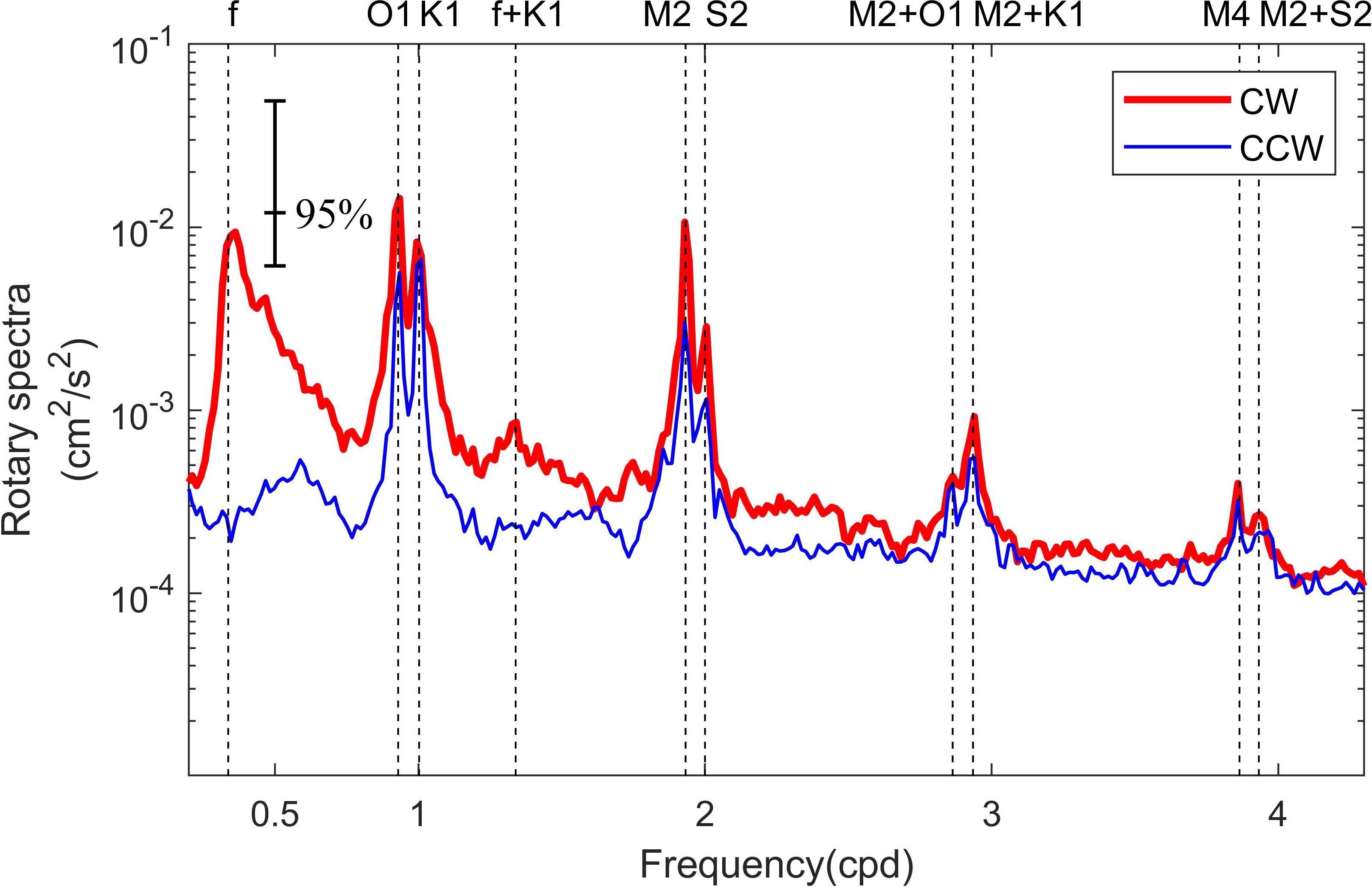
Figure 6. Average rotary spectra of the raw currents from 175 to 740 m for clockwise (red) and counterclockwise (blue) components.
The primary horizontal propagation direction of NIWs is toward the equator. Remotely generated NIWs detected at this observation station are predominantly propagating from higher latitudes. Because the Coriolis frequency increases with latitude, the frequency of NIWs will have a blue shift in most cases, with their energy contained in a broad frequency band (Fu, 1981; Alford and Whitmont, 2007; Xu et al., 2013). In addition, background vorticity also has an influence on the frequency of NIWs. Negative vorticity causes a red shift, while positive vorticity results in a blue shift (Kunze, 1985, 1995). The central frequency band shown in Figure 6 is 0.346–0.361 cpd, with a blue shift of about 3–8% in this region.
Even though the velocity of the diurnal ITs obtained by filtering is small due to the diminutive stratification shear, the 14-day spring-neap cycle can be identified directly from the zonal velocity of diurnal ITs (Figure 7A). Nevertheless, the 14-day spring-neap cycle is not obvious in the meridional component (Figure 7B). The maximum velocity of diurnal ITs is distributed among various depths, implying that the diurnal ITs might be dominated by higher modes. To identity that, the first three baroclinic modes are extracted in this study (Figure 7D). During the whole mooring period, the HKE (Figure 7C) of diurnal ITs fluctuates within a limited range and there is a strong periodic signal change with season. From the middle of December to the end of January, similar cycles and trends are manifested in the HKE of diurnal ITs. However, the cycle period is shortened after February. Different from the results of Shang et al. (2015), which implied that the diurnal ITs were dominated by mode-1 in the west Nansha area, the diurnal ITs at the observation station are mainly dominated by mode-3 for most of the observation period, containing 73% of the diurnal ITs HKE (Figure 7F). Our observation station is located on a slope in the southeast part of the Nansha area where the barotropic currents flowing through can interact with the complex and sloping terrain to generate ITs locally. The energy of high-mode ITs, which cannot propagate over a long distance, generated locally will be found concentrated near the generation place (Alford and Zhao, 2007). Thus, high-mode ITs might have more energy in complex terrain areas. Compared with mode-1 and mode-2, mode-3 changes more frequently showing a shorter cycle. A significant phase difference is shown between the diurnal barotropic currents from TPXO7.2 (Figure 7E) and the diurnal ITs, suggesting that the diurnal ITs are not locally generated.
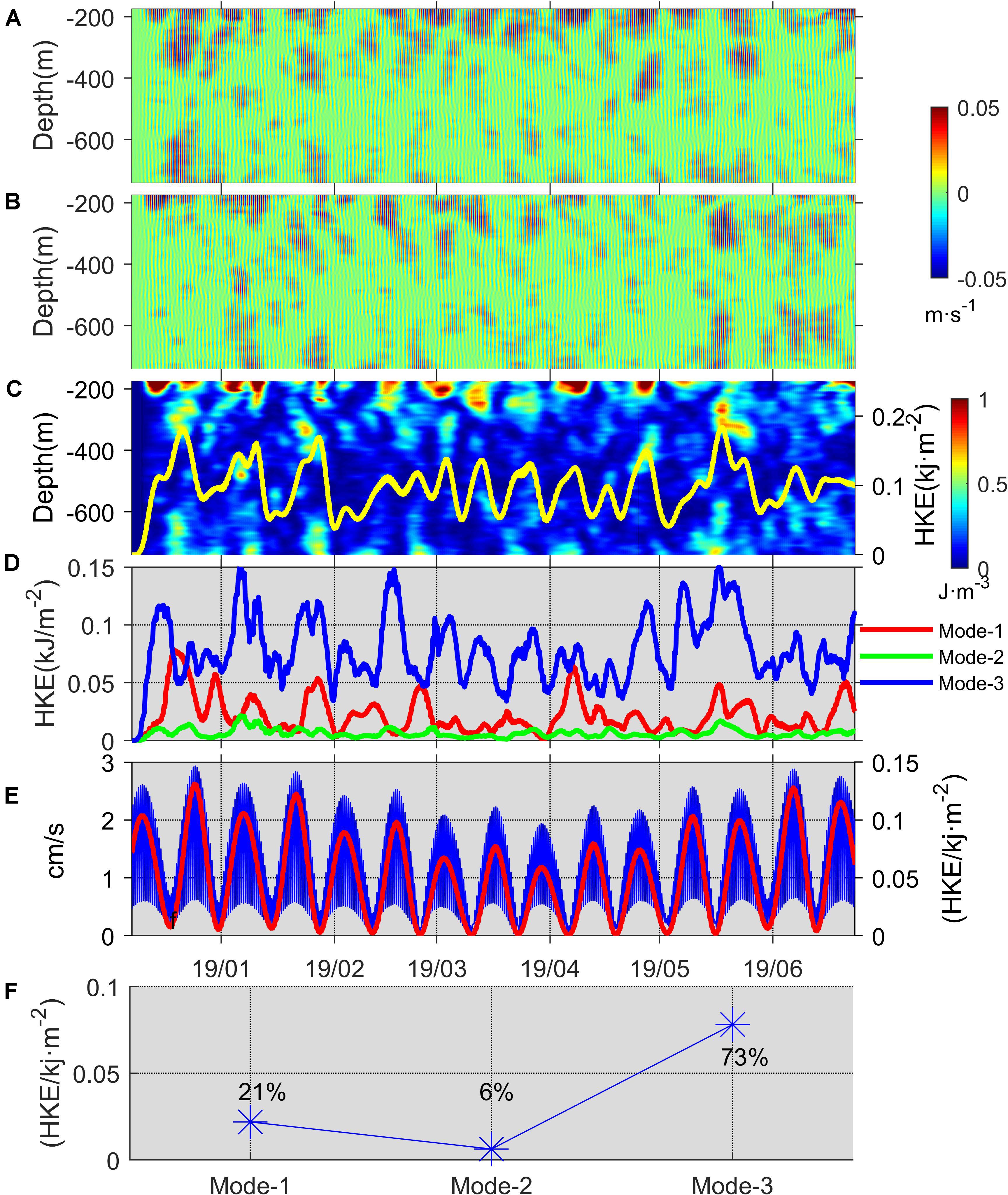
Figure 7. Time series of the zonal velocity of diurnal ITs (A) and meridional velocity of diurnal ITs (B). Distribution of diurnal ITs HKE (C), yellow line for vertical integration. Time series of mode-1 (red), mode-2 (green), and mode-3 (blue) diurnal HKE (D). Barotropic current amplitude (blue) and HKE (red) at diurnal band (E). Horizontal labels mark the start of the month. Proportion of mode-1, mode-2, and mode-3 (F).
Except from March 18 to April 2, there is no obvious 14-day spring-neap cycle shown in the observation period (Figures 8A,B). It is related to the proportion of an incoherent component (93%). When the incoherent component dominates, the ITs are more easily affected by the background field (Xu et al., 2013). Incoherent ITs are caused by a non-linear interaction between varying background conditions and internal wave motions (Xu et al., 2016). Furthermore, the HKE of incoherent ITs can reflect the interaction between the background field and ITs (van Haren, 2004; Alford et al., 2015; Xu et al., 2021). Through harmonic analysis of the ITs, we can extract the coherent ITs, those with astronomical tide frequencies. The incoherent ITs are defined as the residual once the coherent ITs are removed. The coherent parts are 49% and 7% of the diurnal and semidiurnal ITs, respectively. The HKE of semidiurnal ITs (Figure 8C) fluctuates within a limited range at most times, but shows a significant peak on March 25. Likewise, the first three baroclinic modes (Figure 8D) are computed. It can be seen that the semidiurnal ITs are dominated by mode-1 (47%) and mode-3 (34%) mainly (Figure 8F).
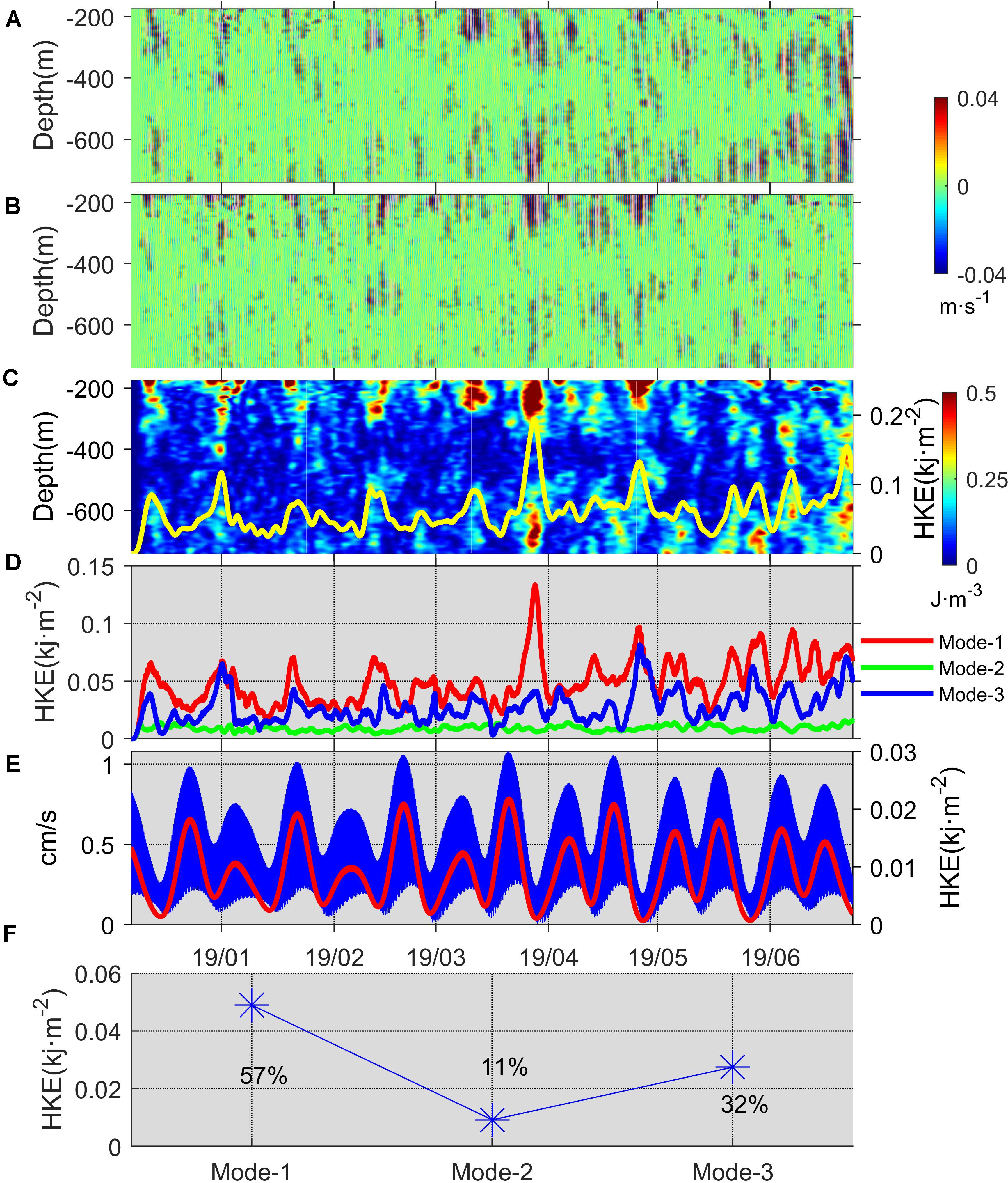
Figure 8. Time series of the zonal velocity of semidiurnal ITs (A) and meridional velocity of semidiurnal ITs (B). Distribution of semidiurnal ITs HKE (C), yellow line for vertical integration. Time series of mode-1 (red), mode-2 (green), and mode-3 (blue) semidiurnal HKE (D). Barotropic current amplitude (blue) and HKE (red) at semidiurnal band (E). Horizontal labels mark the start of the month. Proportion of mode-1, mode-2, and mode-3 (F).
The abrupt increase of semidiurnal ITs (Figures 8C,D) near the end of March might be generated locally or propagated from a distance. High-mode and low-mode ITs will increase simultaneously if ITs are generated locally, while ITs propagated from a distance will show energy concentration on low-mode ITs (Alford and Zhao, 2007). At the end of March, a significant increase in HKE is shown in mode-1 and mode-3, which indicates that local generation is dominant. Time series of barotropic currents in semidiurnal bands from TPXO7.2 (Figure 8E) are also extracted to examine whether the semidiurnal ITs are generated at the observation station. Consistent with diurnal ITs, the phase difference between semidiurnal ITs and barotropic currents is significant, suggesting that the semidiurnal ITs were also not locally generated.
Through a numerical study, Furuichi et al. (2008) found that 85% of the downward near-inertial energy generated by wind forcing will be limited to the mixing layer and dissipated in the upper 150 m. However, Alford et al. (2012) inferred that 12–33% of it will also pass vertically through more than 800 m. Although the data in this study have not covered the area in the upper 150 m, it still has certain significance for the study of NIWs. Different from the diurnal ITs and semidiurnal ITs, NIWs show a wider variation band in velocity as a result of their long cycle of about 71 h (Figures 9A,B). The observed signals of NIWs are intermittent, with the energy propagating both upward and downward.
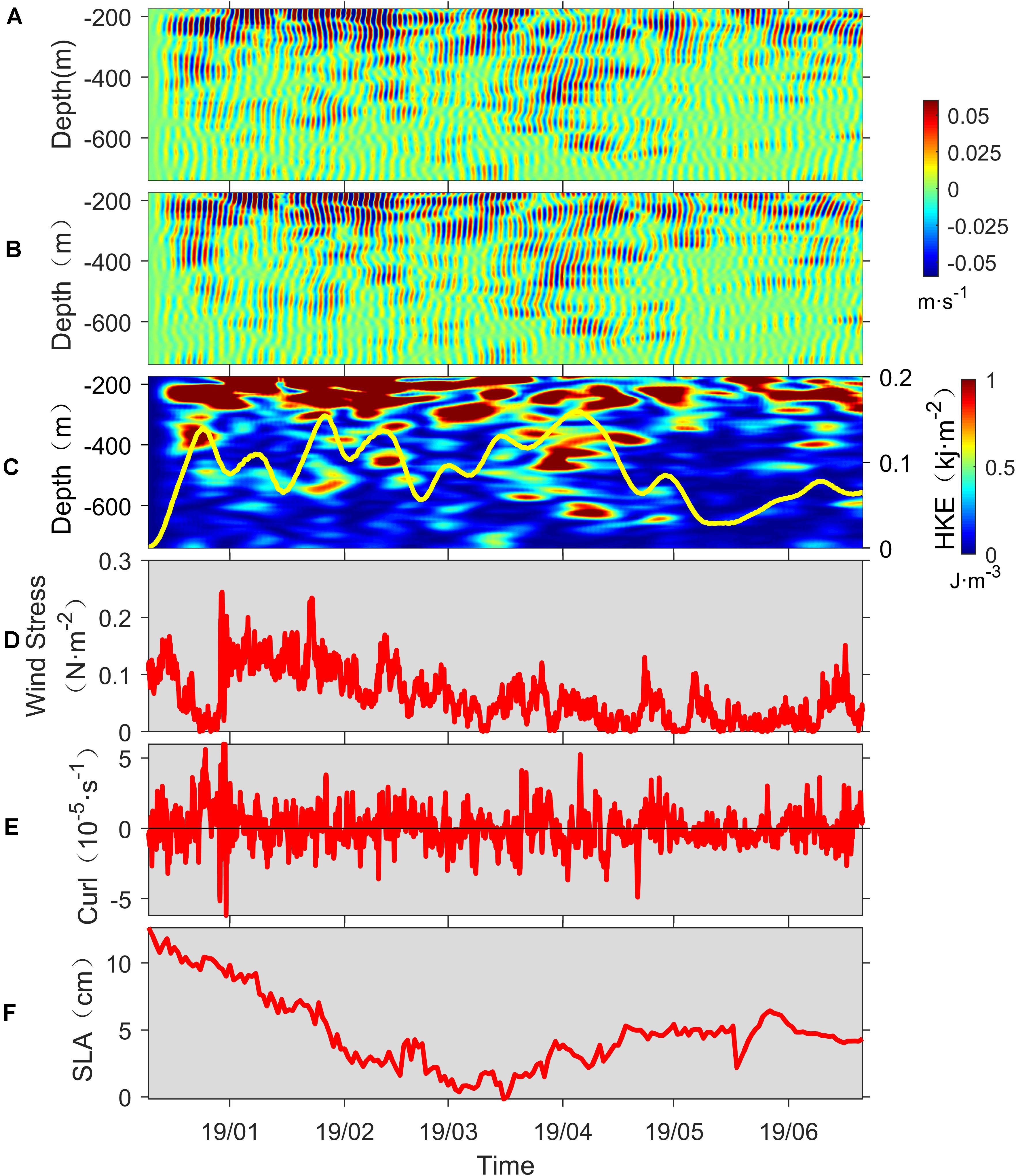
Figure 9. Time series of the WKB-scaled meridional velocity of NIWs (A) and WKB-scaled zonal velocity of NIWs (B). Distribution of WKB-scaled NIWs HKE (C), yellow line for vertical integration. Time series of wind stress (D), wind stress curl (E), and SLA (F). Horizontal labels mark the start of the month.
Compared with semidiurnal ITs, our results showed that the non-linear interaction between NIWs and diurnal ITs was more effective (Figure 6) for the visible peaks at the frequencies of f+O1 and f+K1. NIWs obtain energy more effectively from diurnal ITs than from semidiurnal ITs. The NIW-generating mechanism of geostrophic adjustment has no specific propagation direction. This makes it difficult to discern its contribution to NIWs. NIWs arising from wind forcing and lee waves over the bottom topography can be distinguished by the propagation direction of phase in most cases (Alford et al., 2016). The group velocity of the NIWs is perpendicular to the phase velocity. The phase of NIWs arising from wind forcing propagates upward and the energy propagates downward, while NIWs generated by lee waves over the bottom topography show the opposite character, with the phase propagating downward and energy propagating upward. However, when strong winds with a huge magnitude break out, the NIWs arising from wind forcing propagate to the bottom and reflect upward, then show the characteristics of phase propagating downward and energy propagating upward. In most of the observed depths, the HKE of NIWs propagates downward (Figure 9), which indicates that NIWs at the observation station mainly arose from wind forcing, while the other three mechanisms had little influence.
During the observation period, there were two periods when near-inertial energy was high: from the end of December to the middle of February, and from the middle of March to the beginning of April (Figure 9C). From the end of December to the middle of February, the southern SCS is dominated by the superposition of northeast monsoon and northeast trade wind (Figures 9D,E). In addition, typhoons generate in the SCS frequently, but rarely affect the southern SCS. Thus, in most cases, it is the northeast monsoon period that has the strongest wind forcing in the southern SCS. Wind can provide energy for the near-inertial motions in the ocean-mixed layer, and strong near-inertial energy arises from monsoons during the northeast monsoon period (Liang et al., 2016). From the end of December to the middle of February, due to wind forcing on the sea surface, the near-inertial energy is mainly concentrated in the surface, and the phase of near-inertial velocity mainly propagates upward. However, from the middle of March to the beginning of April, the wind stress intensity is small, the energy arising locally from wind forcing is less, and the energy is mainly concentrated in depths of 200–600 m. However, the phase of near-inertial velocity is still mainly propagating upward, implying that the peaks from the middle of March to the beginning of April might still arise from wind forcing. The lag of calculated energy relative to wind might be due to the phase average required in the calculation process and the low spatial and temporal resolution of wind stress data. In most of the observation period, the SLA (Figure 9F) is maintained within 0–10 cm and the curl (Figure 9E) within −5 × 10⁻⁵ to 5 × 10⁻⁵ s–1, both of which are in the range of moderate or weak SLA and cyclones, defined by Gao et al. (2019). Therefore, the difference between the periods of the propagation process caused by SLA and curl can be ignored. NIWs will propagate to the equator primarily in the horizontal direction; this implies that strong wind events occurring on the north of the observation site can generate a great deal of NIWs, which then propagate to the south.
In section “Near-Inertial Waves,” we found that during the whole observation period, diurnal ITs are dominated by mode-3, while mode-1 only takes up a small part of the energy. This might indicate that the ITs generated from the Luzon Strait have little influence on the eastern Nansha area, or that the diurnal ITs in the eastern Nansha area are not transmitted from the Luzon Strait. Similar to the results of Shang et al. (2015), the semidiurnal ITs, which are dominated by mode-1 and mode-3, show the characteristics of a multimodal structure.
In order to verify our conjecture in section “Near-Inertial Waves” that the peak in NIWs from the middle of March to the beginning of April is due to strong wind events in the north, the ECMWF dataset is used to depict the wind fields in the southern SCS. Figure 10 shows the wind fields on March 14 (Figure 10A) and March 21 (Figure 10B) in the southern SCS. A strong wind event was found in the Mindoro Strait on March 14 and moved westward, then it covered most of the southern SCS on March 21. However, our observation point did not experience the strong wind which higher latitudes experienced. The whole wind process, which lasted from March 14 to March 29, has a good correlation with the strong near-inertial energy observed from the middle of March to the beginning of April (Figure 9C). The propagation of NIWs is very complex. Vertically, the NIWs will reflect when they encounter the thermocline and the sea bottom. Additionally, the downward propagation will be affected by the mesoscale eddies, SLA, and wind stress curls. Horizontally, the remote NIWs triggered in higher latitudes will propagate toward the equator to provide energy for near-inertial activities in lower latitudes.
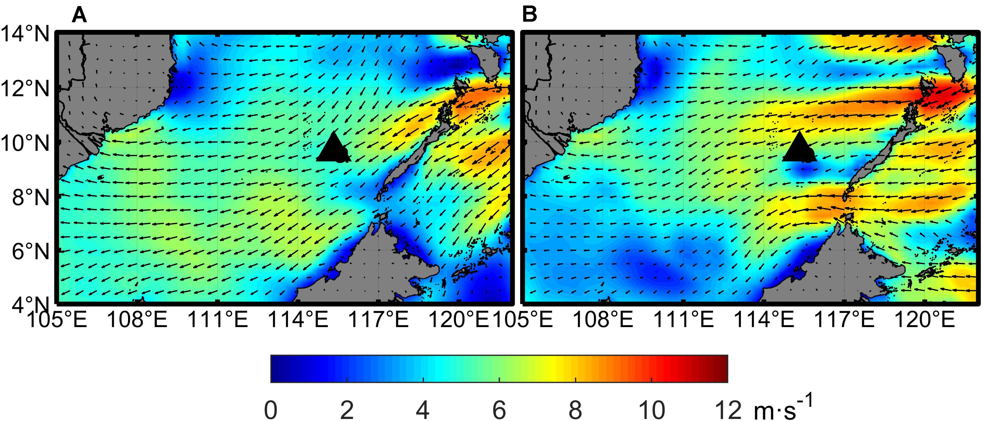
Figure 10. Wind vectors (arrows) and speeds (shaded background color) (m/s) in the southern South China Sea on March 14 (A) and March 21 (B). The black triangle is the mooring station.
Using 7 months of mooring current records, this paper documents the features and temporal variations of ITs and NIWs in the east Nansha area during the observation period. The observed ITs were substantially dominated by O1, K1, and M2, and the energy of clockwise spectra was higher than that of counterclockwise spectra. In addition, the HKE of semidiurnal ITs was smaller than that of diurnal ITs. The diurnal ITs were dominated by mode-3, which accounted for 73% of diurnal HKE, while semidiurnal ITs were dominated by mode-1 (57%) and mode-3 (32%), and the semidiurnal IT energy reached a maximum at the end of March. Coherent diurnal ITs accounted for almost 49% of diurnal ITs, while the coherent portion of semidiurnal ITs was only 7%, causing the semidiurnal ITs to be more susceptible to the background field.
Although the eastern Nansha area is rarely affected by typhoons, the near-inertial energy still mainly arose from wind forcing. The non-linear wave–wave interaction provided a small magnitude of energy for the NIWs, and it was more effective at converting energy from diurnal ITs than from semidiurnal ITs. Horizontal NIW propagation was affected by NIWs generated from other latitudes, and vertical NIW propagation by many factors including topography, thermocline, SLA, mesoscale eddies, and wind stress curl. One of the most important methods to judge whether NIWs arise from wind forcing in other latitudes is to scrutinize whether the energy is limited to the upper layer. The equatorward-propagating NIWs will propagate and dissipate into the deep ocean; their energy is concentrated deeper than the local NIWs.
Although our dataset is coarse and does not cover the full depth, the internal wave structure in the southeastern SCS was well detected by these observations. In the future, more sufficient and comprehensive data will help to obtain a more thorough and precise understanding of internal waves in the whole SCS.
The original contributions presented in the study are included in the article/supplementary material, further inquiries can be directed to the corresponding author/s.
ZZ took part in writing the manuscript draft and result analyses. HX acted as PI supervisor for guiding the whole theoretic diagnoses and revised the manuscript. PV helped to revise manuscript writing and result analyses. QX and XX revised the manuscript and gave advices on manuscript structure. WS and CT helped to collect the data and do raw data quality control. All authors contributed to the article and approved the submitted version.
This study was supported by the National Key R&D Program of China (Grant 2018YFC0309800), the Strategic Priority Research Program of the CAS (Grant XDA13030302), the National Natural Science Foundation of China (Grants 41576006, 41676015, 42076028, and 41704081), and the CAS Frontier Basic Research Project (Grant QYJC201910).
The authors declare that the research was conducted in the absence of any commercial or financial relationships that could be construed as a potential conflict of interest.
Alford, M. H. (2003). Redistribution of energy available for ocean mixing by long-range propagation of internal waves. Nature 423, 159–162. doi: 10.1038/nature01628
Alford, M. H., Cronin, M. F., and Klymak, J. M. (2012). Annual cycle and depth penetration of wind-generated near-inertial internal waves at ocean station papa in the Northeast Pacific. J. Phys. Oceanogr. 42, 889–909. doi: 10.1175/jpo-d-11-092.1
Alford, M. H., MacKinnon, J. A., Simmons, H. L., and Nash, J. D. (2016). Near-inertial internal gravity waves in the ocean. Ann. Rev. Mar. Sci. 8, 95–123. doi: 10.1146/annurev-marine-010814-015746
Alford, M. H., Peacock, T., Mackinnon, J. A., Nash, J. D., Buijsman, M. C., Centurioni, L. R., et al. (2015). The formation and fate of internal waves in the South China Sea. Nature 521, 65–69. doi: 10.1038/nature14399
Alford, M. H., and Zhao, Z. X. (2007). Global patterns of low-mode internal-wave propagation. Part I: energy and energy flux. J. Phys. Oceanogr. 37, 1829–1848. doi: 10.1175/Jpo3085.1
Alford, M. H., and Whitmont, M. (2007). Seasonal and spatial variability of near-inertial kinetic energy from historical moored velocity records. J. Phys. Oceanogr. 37, 2022–2037. doi: 10.1175/jpo3106.1
Benjamin, J., and Shay, L. K. (2010). Near-inertial wave wake of hurricanes katrina and rita over mesoscale oceanic eddies. J. Phys. Oceanogr. 40, 1320–1337. doi: 10.1175/2010JPO4309.1
Duda, T. F., Lynch, J. F., Irish, J. D., Beardsley, R. C., Ramp, S. R., Chiu, C. S., et al. (2004). Internal tide and nonlinear internal wave behavior at the continental slope in the northern South China Sea. IEEE J. Oceanic Eng. 29, 1–27. doi: 10.1109/Joe.2004.836998
Duda, T. F., and Rainville, L. (2008). Diurnal and semidiurnal internal tide energy flux at a continental slope in the South China Sea. J. Geophys. Res. Oceans 113:C03025. doi: 10.1029/2007jc004418
Egbert, G. D., and Erofeeva, S. Y. (2002). Efficient inverse modeling of barotropic ocean tides. J. Atmos. Oceanic Technol. 19, 183–204. doi: 10.1175/1520-04262002019<0183:EIMOBO<2.0.CO;2
Fu, L. L. (1981). Observations and models of inertial waves in the deep ocean. Rev. Geophys. 19, 141–170. doi: 10.1029/RG019i001p00141
Furuichi, N., Hibiya, T., and Niwa, Y. (2008). Model-predicted distribution of wind-induced internal wave energy in the world’s oceans. J. Geophys. Res. Oceans 113:C09034. doi: 10.1029/2008jc004768
Gao, J., Wang, J., and Wang, F. (2019). Response of near-inertial shear to wind stress curl and sea level. Sci. Rep. 9:20417. doi: 10.1038/s41598-019-56822-z
Garrett, C., and Kunze, E. (2007). Internal tide generation in the deep ocean. Annu. Rev. Fluid Mech. 39, 57–87. doi: 10.1146/annurev.fluid.39.050905.110227
Gonella, J. (1972). Rotary-component method for analyzing meteorological and oceanographic vector time series. Deep Sea Res. 19, 833–846. doi: 10.1016/0011-7471(72)90002-2
Guan, S. D. (2014). Near Inertial Oscillations in the Northern Southern South China Sea. Ph.D. Thesis. Qingdao: Ocean University of China.
Guo, P., Fang, W., Liu, C., and Qiu, F. (2012). Seasonal characteristics of internal tides on the continental shelf in the northern South China Sea. J. Geophys. Res. Oceans 117, C04023. doi: 10.1029/2011jc007215
Helfrich, K. R., and Melville, W. K. (2006). Long nonlinear internal waves. Annu. Rev. Fluid Mech. 38, 395–425. doi: 10.1146/annurev.fluid.38.050304.092129
Kunze, E. (1985). Near-inertial wave propagation in geostrophic shear. J. Phys. Oceanogr. 15, 544–565. doi: 10.1016/0198-0254(85)93671-4
Kunze, E. (1995). The energy balance in a warm-core ring’s near-inertial critical layer. Phys. Oceanogr. 25, 942–957. doi: 10.1175/1520-04851995025<0942:TEBIAW<2.0.CO;2
Jan, S., Chern, C. S., Wang, J., and Chao, S. Y. (2007). Generation of diurnal K-1 internal tide in the luzon strait and its influence on surface tide in the South China Sea. J. Geophys. Res. Oceans 112:C06019. doi: 10.1029/2006jc004003
Liang, H., Zheng, J., and Tian, J. W. (2016). Observation of internal tides and near-inertial waves on the continental slope in the northwestern South China Sea. Haiyang Xuebao. 38, 34–42. doi: 10.3969/j.issn.0253-4193.2016.11.003
Liu, Q., Xie, X. H., Shang, X. D., and Chen, G. Y. (2016). Coherent and incoherent internal tides in the southern South China Sea. Chin. J. Oceanol. Limnol. 34, 1374–1382. doi: 10.1007/s00343-016-5171-5
Liu, Q., Xie, X., Shang, X., Chen, G., and Wang, H. (2019). Modal structure and propagation of internal tides in the northeastern South China Sea. Acta Oceanol. Sin. 38, 12–23. doi: 10.1007/s13131-019-1473-1
Qiu, C., Huo, D., Liu, C., Cui, Y., Su, D., Wu, J., et al. (2019). Upper vertical structures and mixed layer depth in the shelf of the northern South China Sea. Cont. Shelf Res. 174, 26–34. doi: 10.1016/j.csr.2019.01.004
Shang, X., Liu, Q., Xie, X., Chen, G., and Chen, R. (2015). Characteristics and seasonal variability of internal tides in the southern South China Sea. Deep Sea Res. Part I Oceanogr. Res. Pap. 98, 43–52. doi: 10.1016/j.dsr.2014.12.005
van Aken, H. M., van Haren, H., and Maas, L. R. M. (2007). The high-resolution vertical structure of internal tides and near-inertial waves measured with an ADCP over the continental slope in the Bay of Biscay. Deep Sea Res. Pt I 54, 533–556. doi: 10.1016/j.dsr.2007.01.003
van Haren, H. (2004). Incoherent internal tidal currents in the deep ocean. Ocean Dyn. 54, 66–76. doi: 10.1007/s10236-003-0083-2
van Haren, H. (2005). Tidal and near-inertial peak variations around the diurnal critical latitude. Geophys. Res. Lett. 32:L23611. doi: 10.1029/2005gl024160
Xie, X. H., Chen, G. Y., Shang, X. D., and Fang, W. D. (2008). Evolution of the semidiurnal (M2) internal tide on the continental slope of the northern South China Sea. Geophys. Res. Lett. 35:13. doi: 10.1029/2008gl034179
Xie, X. H., Shang, X. D., and Chen, G. Y. (2010). Nonlinear interactions among internal tidal waves in the northeastern South China Sea. Chin. J. Oceanol. Limn. 28, 996–1001. doi: 10.1007/s00343-010-9064-8
Xie, X. H., Shang, X. D., van Haren, H., Chen, G. Y., and Zhang, Y. Z. (2011). Observations of parametric subharmonic instability-induced near-inertial waves equatorward of the critical diurnal latitude. Geophys. Res. Lett. 38:L05603. doi: 10.1029/2010gl046521
Xu, Z., Yin, B., Hou, Y., and Xu, Y. (2013). Variability of internal tides and near-inertial waves on the continental slope of the northwestern South China Sea. J. Geophys. Res. Oceans 118, 197–211. doi: 10.1029/2012jc008212
Xu, Z., Liu, K., Yin, B., Zhao, Z., Wang, Y., and Li, Q. (2016). Long-range propagation and associated variability of internal tides in the South China Sea. J. Geophys. Res. Oceans 121, 8268–8286. doi: 10.1002/2016JC012105
Xu, Z., Wang, Y., Liu, Z., Yin, B., McWilliams, J. C., and Gan, J. (2021). Insight into the Dynamics of the Radiating Internal Tide Associated with the Kuroshio Current. J. Geophys. Res. Oceans 126:e2020JC017018. doi: 10.1029/2020JC017018
Keywords: internal tides, near-inertial waves, horizontal kinetic energy, modal decomposition, the southeastern South China Sea
Citation: Zhang Z, Xu H, Vetter PA, Xie Q, Xie X, Song W and Tian C (2021) High-Frequency Motions in the Southeastern South China Sea During Winter–Spring 2018/2019. Front. Mar. Sci. 8:681993. doi: 10.3389/fmars.2021.681993
Received: 17 March 2021; Accepted: 02 June 2021;
Published: 22 July 2021.
Edited by:
Zhiyu Liu, Xiamen University, ChinaReviewed by:
Robin Robertson, Xiamen University Malaysia, MalaysiaCopyright © 2021 Zhang, Xu, Vetter, Xie, Xie, Song and Tian. This is an open-access article distributed under the terms of the Creative Commons Attribution License (CC BY). The use, distribution or reproduction in other forums is permitted, provided the original author(s) and the copyright owner(s) are credited and that the original publication in this journal is cited, in accordance with accepted academic practice. No use, distribution or reproduction is permitted which does not comply with these terms.
*Correspondence: Hongzhou Xu, aHp4dUBpZHNzZS5hYy5jbg==
Disclaimer: All claims expressed in this article are solely those of the authors and do not necessarily represent those of their affiliated organizations, or those of the publisher, the editors and the reviewers. Any product that may be evaluated in this article or claim that may be made by its manufacturer is not guaranteed or endorsed by the publisher.
Research integrity at Frontiers
Learn more about the work of our research integrity team to safeguard the quality of each article we publish.