4DEMON: Integrating 40 Years of Data on PCB and Metal Contamination in Marine Sediments of the Belgian Part of the North Sea

The assessment of historical data is important to understand long-term changes in the marine environment. Whereas time series analyses based on monitoring data typically span one or two decades, this work aimed to integrate 40 years of monitoring and research data on polychlorinated biphenyls (PCBs) and metals in the Belgian Part of the North Sea (BPNS). Multiple challenges were encountered: sampling locations changed over time, different analytical methods were applied, different grain size fractions were analyzed, appropriate co-factors were not always analyzed, and measurement uncertainties were not always indicated. These issues hampered the use of readily available, highly standardized trend modeling approaches like those proposed by regional sea conventions such as OSPAR, named after the Oslo and Paris conventions.Therefore, we applied alternative approaches, allowing us to include most older historical data that have been obtained during the nineteen seventies and eighties. Our approach included reproducible and quality controlled procedures from data collection up to data assessment. It included spatial clustering, data normalization and parametric linear mixed effect modeling. A Ward hierarchical clustering was applied on recently obtained contaminant data, as the basis for a spatial division of the BPNS into five distinct areas with different contamination profiles. To minimize the risk of normalization errors for the metal data analyses, four normalization approaches were applied and mutually compared: granulometric and nickel (Ni) normalization, next to two hybrid normalization methods combining aluminum (Al) and iron (Fe) normalization. The long-term models revealed decreasing trends for most metals, except zinc (Zn) for which three out of four models showed increasing concentrations in all five zones of the BPNS. Offshore sediments contained the lowest normalized mercury (Hg) and cadmium (Cd) concentrations but high arsenic (As) concentrations. Trend analysis revealed a strong decrease in PCB concentrations in the nineteen eighties and nineties, followed by a slight increase over the last decade. The extended timeframe for contaminant assessment, as applied in this study, is of added value for scientists and policy makers, as the approach allows to detect trends and effects of anthropogenic activities within the marine environment within a broad perspective.

Introduction

To evaluate the contamination status of the marine environment, it is important to compare actual concentrations of pollutants with defined values below which no adverse effect is expected, but also to assess and understand how contamination evolves over time. Contaminant trend assessments increase our knowledge on long term human impacts on the marine environment and allow predictions of the near future contamination status. Publications on trend analyses of chemical contamination within European marine sediments consider two approaches: data analysis of monitoring samples repeatedly taken over a long-term period vs. analysis of samples from different depths taken from single sediment cores (e.g., Cundy et al., 2003; Roose et al., 2005; Traven, 2013; Assefa et al., 2014; Everaert et al., 2014; Mil-Homens et al., 2014; Sobek et al., 2015; De Witte et al., 2016; Wafo et al., 2016; Everaert et al., 2017). Typically, trend analyses on monitoring data span at most one to two decades. Sediment core analyses may span a longer period and offer the advantage that no changes in analytical method have to be considered (Yake, 2001), although measured concentrations may be influenced by contaminant degradation and sediment disturbance (Cundy et al., 2003).

To assess the chemical status within the Nord-East Atlantic, the OSPAR commission, named after the Oslo and Paris conventions, continuously evaluates trends in chemical concentrations in marine sediments and biota as well as the potential of current mitigation measures to reach background assessment concentrations (BAC) (e.g., OSPAR, 2017). BAC values indicate whether contamination levels are “near background” (for naturally occurring substances) or “close to zero” (for man-made substances) (OSPAR, 2009). For these assessments, an eminent procedure is applied with a high degree of harmonization and standardization. In brief, the OSPAR assessment on marine sediment contaminants includes sampling guidelines as well as guidelines on the analysis protocols with related quality assessments (OSPAR, 2018, 2019). The data assessment includes a normalization step, taking into account the measurement uncertainties, followed by a trend analysis based on a linear model (for a period of 5–6 years) or based on a smooth model (for data spanning 7 years or more). Data with high uncertainty are excluded from the assessment or their weight is reduced. A normalization step is essential, since contaminant concentrations in marine sediments depend on the pollution level but also on the natural variability in sediment granulometry (i.e., grain size distribution) and mineralogy (i.e., mineralogical composition). Fine sediments, which are mainly composed of clay minerals, present high binding capacity leading to higher contaminant concentrations, compared to coarse sediments (Loring, 1991). Two normalization approaches are widely applied: granulometric and geochemical normalization. The first approach consists of sieving and isolating the clay fraction, i.e., the <63 μm fraction which is the most widespread monitoring fraction used, to reduce the differences in granulometric composition (OSPAR, 2018). The second approach relies on the use of a proxy to reflect the binding capacity of the sediment in function of its mineralogy and grain size. This proxy or co-factor has to be a conservative element, like Aluminum (Al), which reflects the clay mineral content and whose content is unaffected by other contaminant inputs (Herut and Sandler, 2006).

For the Belgian part of the North Sea (BPNS), monitoring of hazardous substances started in 1971 with the project named “Project Mer-projekt zee” (PMPZ), where PCBs, pesticides and metals were analyzed in marine waters, sediments and biota. Since then, a long, more or less continuous series of research and monitoring projects has been conducted, all reporting on the chemical contamination level of the BPNS. The recent 4DEMON (4 Decades of Belgian Marine Monitoring) project has compiled a long term dataset on contamination, eutrophication and acidification on the BPNS since the 1970s (Lagring et al., 2018), comprising as much data as possible, gathered and rescued from the multiple projects and data originators over time. The integrated 4DEMON dataset offers a unique set of contamination data in marine sediments.

To our knowledge, no chemical trend analysis spanning a four decades period has ever been published within peer reviewed publications. A major problem is that by incorporating historical data from different data originators, we encountered multiple issues, which hampered the use of existing assessment methods. Over the 40 years’ time span, the sampling frequency of marine sediment monitoring has changed and sampling locations were altered, which inhibited a 40 years trend assessment on individual locations. A scientifically based spatial clustering was needed to combine data of multiple locations and to allow for a time series analysis of hazardous substances in spatially (a priori) defined zones of the BPNS.

A second issue is the variability of grain size fractions (<37, <63, <500, <2,000, <10,000 μm) on which contaminant analyses have been performed, emphasizing the need for other data normalization procedures besides grain size normalization. OSPAR assessments use aluminum (Al) for the evaluation of metals, as the metal content of fine sediments is related to major elements of the clay fraction such as Al (OSPAR, 2018). For organic contaminants, Total Organic Carbon (TOC) is used as co-factor, since organic contaminants have strong affinity for organic carbon (OSPAR, 2018). Within the 4DEMON dataset, Al was found to be rarely measured in the seventies, hampering its applicability when trying to retain as much metal concentration data as possible over the four decades. Therefore, in the present study alternative normalization procedures have been developed and applied.

Thirdly, the applied analytical methods have changed over time, which most likely results in shifts in the measured contaminant concentrations, partly masking the real trends. This may be overcome by analyzing samples in duplo by means of both old and new methods (West et al., 2017). However, this approach was not applicable to our datasets, as old measurement and extraction instrumentation were no longer operational, and samples were no longer available. Therefore, a mathematical extrapolation and correction (modeling) solution was developed. It is important to note that changes in co-factor analysis methods may equally induce contaminant concentration shifts. Finally, no or little information was available on measurement uncertainty for the historical contaminant data recovered from different projects, prohibiting the integration of measurement uncertainty in the applied models.

Given these constraints, the current procedures for time trend analysis as applied by OSPAR or within other peer-reviewed publications could not be used for the 4DEMON dataset. This paper presents a unique approach to assess more than four decades of PCB and metals monitoring data, in which spatial clustering, alternative normalization approaches and parametric trend modeling are combined to gain insight in long-term trends in PCB and metal contamination in marine sediments of the BPNS. Our approach included reproducible and quality controlled procedures from data collection up to data assessment. Accuracy is reached by applying tailored made quality control algorithms based on quality flags and acceptance thresholds as well as established statistical algorithms based on statistical significances.

Materials and Methods

To develop long term trends on metals and PCBs in the marine environment of the BPNS, a multi-step approach was applied, including data collection and data quality control, spatial clustering of sampling locations, development and validation of normalization approaches as well as the generation of linear mixed effect models. A flow chart of this process is presented within Figure 1.

FIGURE 1

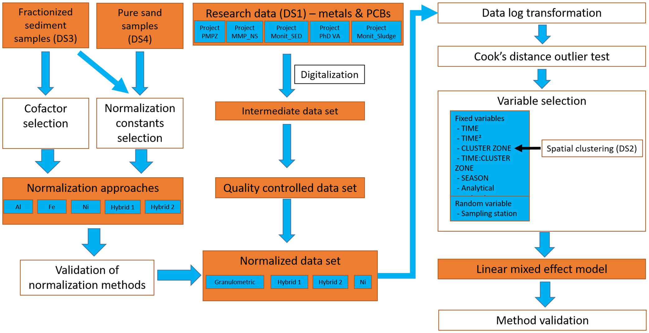
Figure 1. Flow chart of the data process procedures including (1) development of normalization approaches (left), compilation of quality checked datasets (center) and trend modeling (right). Actions are given in uncoloured textboxes. Samples, datasets and results are presented in orange textboxes.

Data Collection and Quality Control

Four datasets have been used: (Dataset 1- DS1) the main dataset for trend modeling as compiled during the 4DEMON project, spanning four decades (1971–2015) of marine monitoring data at the BPNS; (Dataset 2- DS2) a subset, spanning the period 2007–2011, which is used for the spatial clustering; (Dataset 3- DS3) a number of fractionized sediment samples taken in March 2015, to determine optimal co-factors; and (Dataset 4- DS4) a number of pure sand samples, gathered in the most offshore zone of the BPNS in the period 2008–2014, to determine the normalization constants.

The main dataset (DS1) contains PCB and metal data originating from the pioneering PMPZ project (1971–1975), which was continued within the Monitoring Master Plan for the North Sea (MMP_NS; 1978–1983), and the still ongoing OSPAR monitoring program (MONIT_SED, 1979–2015). Contaminant data were further obtained from several monitoring projects related to the effects of human activities at sea, such as dredge spoil disposal and sand extraction (Monit_Sludge, 2004-present), and from a Ph.D. on metal contamination at the BPNS and the Scheldt Estuary (Van Alsenoy, 1993). Other short term project data were included in the 4DEMON digitalization process, but were not used in the current trend analyses due to data comparability restrictions. To be fit for inclusion in the data assessment, only metal data obtained by a total digestion method were retained. Further, only sediment samples collected by a Van Veen grab were considered and project data were not withheld in case not all relevant metadata could be retrieved. Supplementary Table 1 provides an overview of the number of records, projects and periods covered that have been used for the trend analyses. The total dataset is digitally available (4DEMON, 2020).

After compilation of the main dataset, metadata and concentration values were quality checked before performing any statistical analyses. Station locations and analysis methods were carefully verified and corrected when required. For each contaminant, automated and visual screening were performed to identify suspect values. Unrealistic out-of-range as well as zero, negative and missing values were discarded from the final dataset. Values below detection limits were set to detection limit values, duplicates were removed and sample replicates were aggregated by average. The final dataset for the long-term trend assessment comprised 1615 sediment samples taken at 162 sampling locations in the BPNS (Figure 2A). The PCB time series counted at minimum 450 values for CB153 and around 950 values for other PCBs. Metals time series contained between 994 and 1469 records.

FIGURE 2

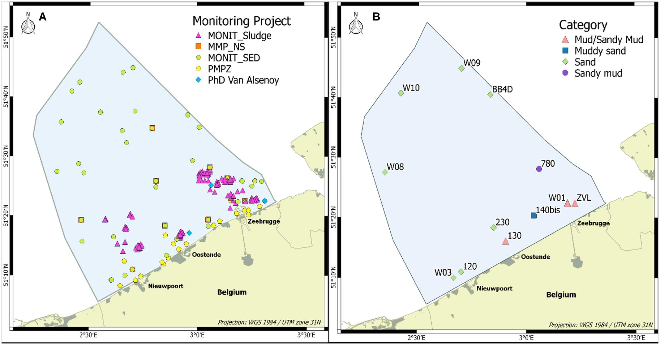
Figure 2. (A) Overview of all sampling locations of the main dataset DS1 (1971–2015). (B) Overview of samples of DS3 used as equally polluted samples in the co-factor analysis (March 2015) and the pure sand samples (W08, W09, W10) of DS4 used for background normalization constant determination (2008–2014).

Spatial clustering was based on a small subset of the 4DEMON contaminant dataset (DS2), containing 443 samples, for which concentrations of PCBs and metals from the sieved fraction 0–63 μm were available. We assume that over such a short period, the contaminant concentrations did not change significantly over time.

To select co-factors following the procedure of Smedes and Nummerdor (2003), sediment samples taken at nine locations within the BPNS in March 2015 with a Van Veen grab (0.1 m²) were used (DS 3) (Figure 2B). Based on the mud (grain size <63 μm), sand (grain size between 63 and 2000 μm) and gravel (grain size >2000 μm) content, samples were classified as mud or sandy mud (>50% grain size <63 μm), muddy sand (10–50% grain size <63 μm) and sand (<10% grain size <63 μm). This categorization was proposed by Rees et al. (2007) as adopted from Folk (1954).

For the determination of normalization constants, three locations at the outer border of the BPNS (W08, W09 and W10) were selected that may be considered as pure sand locations, all having less than 0.01% in the <63 μm fraction (Figure 2B). Metal concentrations from those unsieved samples were considered (DS4).

Spatial Clustering

Throughout four decades of marine monitoring at the BPNS, sampling locations varied over time. To assess real long-term trends in PCB and metal concentrations, we aggregated diverse sampling locations into spatial cluster zones, each characterized by specific contamination and sediment profiles.

First, a Ward hierarchical clustering (Ward, 1963) was applied on the samples of DS2 (the 2007–2011 subset; <63 μm sediment fraction), based on center-scaled concentrations of PCBs and metals with Euclidean distances as similarity measure, using R-function hclust (R Core Team, 2018).

In a second step, a Principal Component Analysis (PCA) was performed, which reduces the number of variables into new uncorrelated variables (principal components). This gives additional information on associated contaminant patterns, where closely positioned variables are more correlated. The PCA was applied on center-scaled PCB and metal concentrations from DS2, using R software function PCA from FactoMineR package (Lê et al., 2008).

Finally, we combined the information from the PCA with the Ward clustering group characteristics and known information on sedimentology (Hademenos et al., 2018) to delineate five spatial zones in which the sampling locations from the main dataset could be grouped for the overall trend analyses.

Normalization

Over 40 years monitoring, contaminant concentrations originated from different sediment fractions with different grain sizes. Moreover, parameters currently used as co-factors were not always analyzed, stressing the need for alternative normalization procedures. Within a first model, only granulometric normalization was applied, i.e., taking into account contaminant concentrations measured on the <63 μm fraction. The other approaches are based on geochemical normalization. The use of a co-factor for normalization purposes assumes that the concentration of the studied contaminant changes proportionally to the co-factor (the normalizing element) in sediments that are equally polluted, as its concentration varies with changing mineralogy and particle size (Loring, 1991). The linear regression between contaminant and co-factor concentration is illustrated in Figure 3 (Smedes et al., 1997).

FIGURE 3

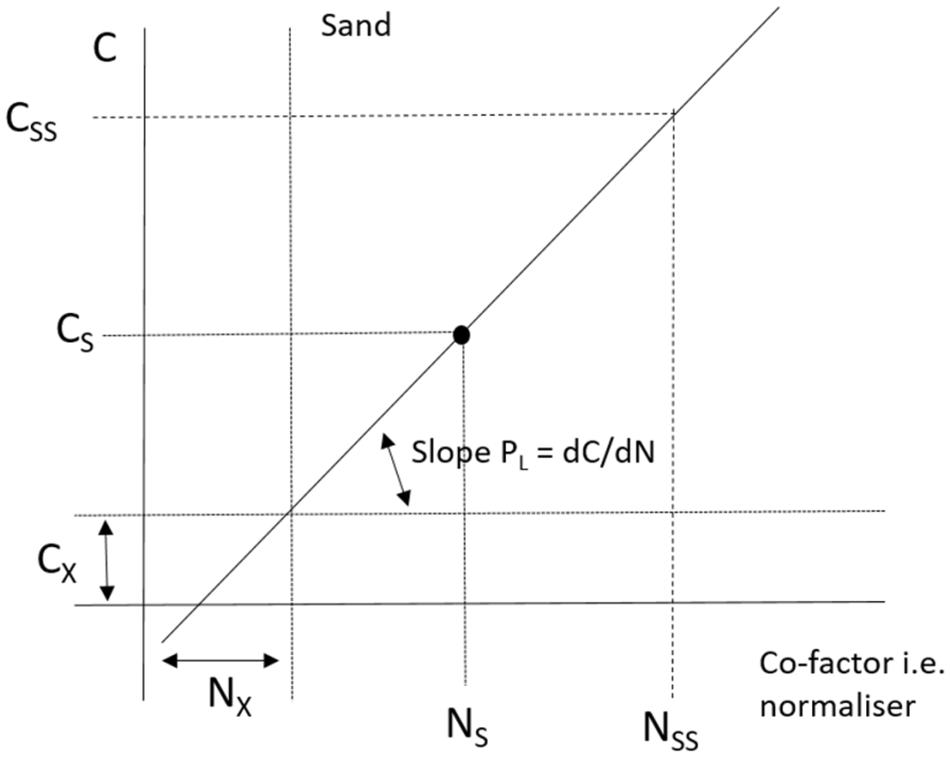
Figure 3. Regression between the contaminant C and the cofactor N (redrafted from Smedes et al., 1997, with permission), with C_S and N_S the measured contaminant and co-factor content, C_SS and N_SS the standard reference contaminant and co-factor content, and C_x and N_x the contaminant and co-factor content in pure sand.

Cs and Ns represent the measured contaminant and co-factor contents, whereas Cx and Nx represent the contaminant and co-factor contents in pure sand, respectively. Cx and Nx represent the “pivot point” from which all sample sets will originate, regardless their contamination level (OSPAR, 2015).

$$\frac{dC}{dN}=\frac{C_s-{\mathrm{C}}_{\mathrm{x}}}{N_s-N_x}(1)$$

The extrapolation to the standard reference co-factor content Nss follows the same slope, resulting in a general expression for the standardized reference contaminant concentration C_SS:

$$C_{ss}=\left(C_s-C_x\right)\frac{N_{ss}-N_x}{N_s-N_x}+C_x(2)$$

Normalization is performed toward a “standard seafloor” with co-factor content Nss. The resulting standardized contaminant levels C_SS can be compared irrespectively of their granular distribution and mineral composition, meaning that samples with the same C_SS value are equally polluted (Smedes and Nummerdor, 2003).

When the measured co-factor value Ns is similar to its background value in pure sand (Nx), the denumerator Ns-Nx approaches zero in Eq. 2 and normalization procedures may lead to enhanced measurement uncertainties on the normalized data. Within normal OSPAR assessments, this issue is counteracted, as most data are obtained on the <63 sediment fractions, which usually results into high co-factor values, and measurement uncertainties are included in the final model, leading to exclusion or weight downsizing of data with larger uncertainties. This approach applied to the 4DEMON data would especially have excluded or downsized all data measured on the <2,000 μm sediment fraction, meaning that mainly the older historical data would have been excluded (as less data were analyzed for the <63 μm fraction in the seventies and eighties), while the project and this paper specifically aim to include these historical data. Moreover, the OSPAR assessment normally uses Al as co-factor, but Al was rarely analyzed on the sediment samples in the seventies.

To be able to include the older historical data and to avoid the introduction of outliers, we developed a project-specific normalization approach. This included: (1) the selection of appropriate co-factors, (2) the determination of good normalization constants, (3) the shaping of the final normalization methods, and (4) the validation of the proposed geochemical normalization methods.

Co-factor Selection

As shown in Figure 3, a linear relationship should exist between the contaminant concentration and the co-factor concentration for equally polluted samples, i.e., samples that have the same normalized contaminant concentration Css (Smedes and Nummerdor, 2003). For PCBs only TOC was tested as co-factor, while for metals three of the commonly used co-factors (Al, Fe and TOC) were tested for their goodness of fit. In addition, we also tested Ni as co-factor for metals, although Ni is not inherently related to the clay content. Linear regressions were deduced for each of the contaminants against the 4 potential co-factors, based on equally polluted samples, and corresponding correlation coefficients R² were calculated.

Equally polluted samples were created by fractionation of the sediment samples of DS3 (sampled in March 2015 at nine locations in the BPNS) into different grain size fractions. All samples were sieved in subsamples, applying an automatic sieving procedure in which seawater from the sampling location is pumped over the sieves. The water passing the sieves is led to a flow-through centrifuge that retains the fine particles and the effluent is returned to the sieves by a peristaltic pump (OSPAR, 2018). First, a 2,000 μm sieve was used to remove the larger sediment particles, withholding the <2,000 μm fraction as fraction 1. Part of fraction 1 was sieved over a 63 μm sieve and part of the fraction <63 μm (fraction 2) was further sieved over a 20 μm sieve, leading to fractions 3 (0–20 μm) and 4 (20–63 μm). The larger fraction >63 μm was ultrasonicated for at least 3 h and further sieved on a sieving tower, leading to five fractions: 500–2000 μm, 250–500 μm, 125–250 μm, 63–125 μm and <63 μm (fractions 5–9, respectively). A schematic overview is provided as supplementary information (Supplementary Figure 1).

The particle size distribution of the total sample was measured using a Malvern Mastersizer 2000 laser diffractometer with Hydro 2000G wet sampling system. Each individual fraction was analyzed on metals, PCB and TOC content. Analyses of metals and TOC were performed as described by De Witte et al. (2016). Briefly, a wet extraction with a mixture of HClO4, HNO3 and HF as digestion solvent was applied for metal analysis followed by determination on inductively coupled plasma-optical emission spectrometry (ICP-OES) or inductively coupled plasma-mass spectrometry (ICP-MS). Hg was determined after dry combustion followed by Au-adsorption and atomic absorption spectrometry (AAS)-quantitation using an advanced mercury analyzer (AMA). TOC analysis was based on dichromate-sulphuric acid oxidation, followed by back-titration with Mohr’s salt. For the PCB analysis, 7 congeners (IUPAC numbers CB28, CB52, CB101, CB118, CB138, CB153, and CB180) were determined. Freeze dried samples were analyzed by pressurized liquid extraction (PLE) with hexane:acetone (3:1), with florisil added to the PLE-cell for clean-up. The extract was desulfurized by activated copper, followed by an additional clean-up on deactivated and acidified silica. Samples were analyzed by gas chromatography (GC)-ion trap mass spectrometry (MS) with separation of PCBs on a TR-PCB 8MS column (Thermo, 50 m, 0.25 mm, 0.25 μm).

Normalization Constant Selection

Regional specific values for the contaminant and co-factor concentrations Cx and Nx were determined for pure sand samples, gathered between 2008 and 2014 at 3 offshore locations in the BPNS. Following the OSPAR protocol, background concentrations for the northern part of the convention area are currently expressed as values normalized to 2.5% TOC (OSPAR, 2018). We used this reference value to deduce the regional specific standard seafloor level Nss for the co-factors Al, Fe and Ni. Linear regressions of Al, Fe and Ni were built against TOC for the 9 equally polluted sieved fractions for each of the nine locations sampled in March 2015. The standard seafloor values are determined as the average of co-factor concentrations deduced from each of the 9 regression sets at TOC equal to 2.5%. The linear regressions for Ni are presented in Figure 4.

FIGURE 4

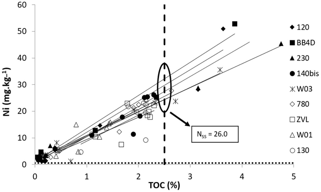
Figure 4. Regression lines of equally polluted samples for Ni vs. TOC to determine Nss (at TOC 2.5%).

The normalization constants Cx and Nx in Eq.2 are also dependent on the analytical method. A total digestion method leads to higher contaminant and normalizer concentrations than a weak digestion method, resulting in larger Cx and Nx values (OSPAR, 2018). Most metal data in sediments from the BPNS have been obtained by total digestion methods. The contaminant-co-factor regressions on equally polluted samples were also determined using total digestion methods. The datasets using weak digestion methods were not included in the trend modeling.

Adapted and New Approaches for Metal Normalization

High pivot point values (Cx/Nx) may lead to high analytical errors and even unrealistic values for Eq. 2 when Cs<Cx or Ns is close to Nx (see further). To overcome these limitations, four different normalization approaches were evaluated and selected for the final trend assessments. One metal normalization procedure was based on granulometric normalization (<63 μm). To tackle the lack of measurement uncertainty data, two normalization procedures relied on multi-parameter normalization with Al and Fe as co-factors (hybrid 1 and hybrid 2). The use of Ni as normalizer within the fourth modeling approach was a pragmatic choice, as in contrast to Al, Ni is not a main constituent of clay.

Granulometric normalization

As normalization is obtained by sieving the sample prior to analysis, contaminant concentrations can be presented, without further recalculations. Only data for samples sieved at 63 μm (<63 μm fraction) were selected and used for trend modeling.

Hybrid normalization 1

The hybrid normalization 1 is based on the general model for geochemical normalization (Smedes et al., 1997) in which two normalized contaminant concentrations are calculated individually, each with a different co-factor, and the results are combined under a deviation range criterion. Relying on Al and Fe as suitable co-factors for the BPNS regional domain, we normalized metal values toward Al and Fe separately (Eq. 2), after which averages of the two standardized metal concentrations are calculated. To exclude potential outliers, the standardized concentrations of Al or Fe not ranging within a defined percentage around the average (arbitrary set at 50%) were discarded from the normalized dataset for the trend modeling. These out-of-range values may be due to analytical errors, to samples that are extremely more or less polluted or derived from areas with different geology, which induces normalizer deviation from linearity regression to contaminants (Grant and Middleton, 1998). The Al-Fe normalization can thus be expressed as follows:

Normalization to Al:

$$C_{ss.AL}=\left(C_s-C_x\right)\frac{N_{SS.AL}-N_{x.AL}}{N_{s.AL}-N_{x.AL}}+C_x(3)$$

Normalization to Fe:

$$C_{ss.FE}=\left(C_s-C_x\right)\frac{N_{SS.FE}-N_{x.FE}}{N_{s.FE}-N_{x.FE}}+C_x(4)$$

Normalization to a combination of Al and Fe:

$$C_{ss.AL-FE}=\frac{C_{ss.AL}+C_{ss.FE}}{2}(5)$$

With a deviation range criterion given as:

$$0.5C_{ss,Al-Fe}<C_{ss.AL},C_{ss.FE}<1.5C_{ss,Al-Fe}(6)$$

Hybrid normalization 2

Hybrid normalization 2 more or less follows the same approach as hybrid 1 with a combination of Fe and Al, but selects alternative individual or combined normalization models when the hybrid normalized value falls outside the fixed deviation range (similar criterion of 50% around the average). Either C_SS,AL (Eq. 2), C_SS,FE (Eq. 3), or C_SS,AL–FE (Eq. 4) will be selected, dependent on cut off conditions set for the Al and Fe terms (N_s-N_x)) in Eq. 1. An indirect cut off condition for (C_S-C_x) is included, since time trend modeling is performed on log transformed normalized data, hence discarding negative normalized values. The hybrid normalization 2 can be expressed as follows:

$$C_{ss}=\{\begin{array}{cc}\hfill \mathrm{\varnothing },& (N_{s.FE}-N_{x.FE})\le 0and(N_{s.AL}-N_{x.AL})\le 0\hfill \\ \hfill C_{ss.AL},& (N_{s.FE}-N_{x.FE})\le 0and(N_{s.AL}-N_{x.AL})>0\hfill \\ \hfill C_{ss.FE},& (N_{s.FE}-N_{x.FE})>0and(N_{s.AL}-N_{x.AL})\le 0\hfill \\ \hfill Inf,& C_{ss.FE}=Infand{C}_{ss.AL}=Inf\hfill \\ \hfill C_{ss.AL-FE},& C_{ss.FE}<3C_{ss.AL}and{C}_{ss.AL}<3C_{ss.FE}\hfill \\ \hfill C_{ss.AL},& C_{ss.FE}\ge 3C_{ss.AL}or{C}_{ss.AL}\ge 3C_{ss.FE}and\hfill \\ & (N_{s.AL}-N_{x.AL})>(N_{s.FE}-N_{x.FE})\}\hfill \\ \hfill C_{ss.FE},& C_{ss.FE}\ge 3C_{ss.AL}or{C}_{ss.AL}\ge 3C_{ss.FE}and\hfill \\ & (N_{s.AL}-N_{x.AL})<(N_{s.FE}-N_{x.FE})\hfill \end{array}$$

Ni normalization

Although Ni is not a main constituent of clay, the contaminant-co-factor regressions on equally polluted samples of the BPNS revealed good regressions between Ni and other metals, suggesting its fit for use for normalization at the BPNS. Moreover, Ni values in marine sediments of the BPNS are limitedly impacted by anthropogenic sources. For example, at sampling location ZEB (N 51.357, E 3.152) on the BPNS, annual variability was very high for most metals, e.g., between 22 and 192 μg.kg^–1 for Hg in the <63 μm fraction sampled in 2009–2013. This variation is related to the influence of the tide on the type of mud that is sampled (freshly deposited sediment vs. Holocene consolidated mud; Fettweis et al., 2009), revealing clear effects of industrial pollution. On the contrary, Ni was one of the contaminants with little variation (21–26 mg.kg^–1 in the <63 μm fraction), indicating the limited influence of anthropogenic pollution. Due to the lack of other available normalizers (such as TOC, Al and Li) in the 1970s, modeling with Ni as normalizer was included to enable the analysis of trends starting from the early seventies. Normalization procedures hybrid 1 and hybrid 2 could only be applied on timelines starting in 1979.

Validating the Metal Geochemical Normalization Methods

The variability between the three methods of metal geochemical normalization was examined on the sample sets of the nine equally polluted samples from the BPNS (period 2008–2014). Ni normalization and hybrid normalization approaches 1 and 2 were also compared to the normalizations based on Al and Fe alone. After normalization, fractionated subsamples (different sediment size classes) from the same location should result in comparable metal concentrations. As a consequence, a good normalization method should result in low interquartile ranges (IQR), low absolute differences between mean and median (reduced skewness) and low number of outliers. A value is considered to be an outlier if it is lower than the first quartile minus 1.5x IQR or higher than the third quartile plus 1.5x IQR. For the five geochemical normalization approaches and each of the seven studied metals (As, Cd, Cr, Cu, Hg, Pb, and Zn), the above mentioned variables were determined for each individual sample and the average (IQR, mean-medium difference) or sum (number of outliers) of all nine samples was calculated. Due to the application of cut-off values when Ns-Nx <0, some values were discarded.

Linear Mixed Effect Models for Long-Term Trend Analyses

In order to assess spatial and temporal distribution of PCBs and metal contaminants in marine sediments across the BPNS, we opted for linear mixed effects models. Approaches relying on linear mixed effects model are prescribed and widely used by the OSPAR MIME (OSPAR, 2008) community for their quality assessments. However, OSPAR MIME suggests the use of a smooth model is function of time as fixed effect and three random effect terms. In our case, we wanted to include as much historical data as possible, which means data inhomogeneous in time, location and analytical method. This unfortunately prevented the suggested OSPAR model to be applied as such to our data.

Linear mixed effect models were applied, using a parametric trend modeling procedure. This allowed us to address the metadata diversity issues by including sampling location, season and analytical method as descriptive parameters, in order to discriminate the effect of variable changes from the real effective modeled trends, i.e., the evolution in contaminant concentrations in time and space. This is particularly the case for analytical method switches in the laboratory, which may be reflected in shifts in the observed contaminant concentrations over time. The fact that different laboratory methods seldom overlap in time makes it difficult to evaluate whether differences are due to laboratory effects or to real changes. In general, concentrations have been measured using the same analytical method for more than 5 years. For each analytical method (period), we observed that the related time trends for most of the contaminants (especially normalized concentrations) followed similar slopes when changing from one method to another. We thus assume that a laboratory effect only implies a level shift (changes in the intercept) but no real trend changes (changes in slope over time). Therefore, the analytical method was included as explanatory variable without adding an interaction term between time and analytical method, thus limiting the complexity of the models. The full optimal mixed-effects models we applied can be described as follows:

$$Y=\mathrm{\alpha }+{\mathrm{\beta }}_{1}t+{\mathrm{\beta }}_2{t}^2+{\mathrm{\beta }}_{3}CLUS{T}_i+{\mathrm{\beta }}_{4}SEASO{N}_j\mathrm{\hspace{1em}}+{\mathrm{\beta }}_{5}AM{D}_k+s_{(l)}+\mathrm{\epsilon }(7)$$

where

- Y: the natural log transformed normalized contaminant concentration in sediment sampled at i^th cluster zone CLUST during j^th season SEASON, measured with the k^th analytical method AMD at l^th station s at time t in years.

- α: the mean concentration level at the start of the monitoring period

- β₁: the mean slope for the linear time trend

- β₂: the mean slope for the quadratic time trend

- β₃: the mean slope for CLUST at i^th cluster zone

- β₄: the mean slope for SEASON at j^th quadrimester

- β₅: the mean slope for AMD at k^th analytical method

- s_(l): the random effect associated with the l^th sampling station

- ε : The error term associated with the above described contaminant concentration

We assumed that s_(l) and ε are independent and that their distributions follow normal distributions of mean 0 and standard deviation σ_s and σ_ε. Log transformation of the contaminant concentrations is needed, so the model residuals follow a normal distribution and to comply with normality conditions necessary to make the fitted model valid. Stations (locations) are included as random effect to capture the spatial correlations between contaminant levels in sediments sampled at same location. Given that sediment contaminant concentrations at one location over several years are expected to be more similar compared to concentrations in the sediment at other locations, each location is assigned a different random intercept value that is estimated by the mixed-effects models. We introduced sampling season, spatial zone and analytical method as fixed effect terms in the full optimal mixed effect model, to evaluate how pollution concentrations are evolving over time. Seasons are defined as quadrimesters. An interaction term between time and zones is added to allow different trends/slopes per cluster zones.

Mixed-effect models were fitted on the natural log-transformed concentrations of each PCB congener with granulometric normalization (i.e., solely sediment fraction 0–63 μm). For the 7 selected metals, mixed-effect models were fitted to log-transformed data, based on the four normalized procedures, i.e., granulometric normalization (0–63 μm granular fraction), normalization methods Hybrid 1 and 2 and Ni normalization. Prior to model fitting, we eliminated influential outliers based on Cook’s distance, which calculates the impact of each data point on the regression analysis. We arbitrary use a cut-off value of 0.2 to discard outliers from the modeled datasets, based on data interpretation with a subset of data.

Model fitting was deduced from restricted maximum likelihood (REML) estimations using R function nmle:lme (Pinheiro et al., 2018). Starting from the full optimal mixed effect models (Eq. 7), fixed variables were selected by means of the maximum likelihood estimation (ML) via the R lme4:drop1() function (Bates et al., 2015), which allows for single term deletions for nested models and likelihood ratio tests (LRT) based on a χ² statistic. All remaining terms were significantly different from 0 at the 5% level. The total reduction (or increase) percentages were deduced for each of the contaminants and normalization methods.

Model validation as described by Zuur et al. (2009) was performed on normalized residuals to verify homogeneity of variance and independence. In some cases, homogeneity and independence could be improved. To reduce the inhomogeneity on residuals spread across analytical methods, which was sometimes observed, we tried to add a fixed variance structure nmle:varIdent() to the model (Pinheiro et al., 2018) to produce different standard deviations per method. However, this did not change the fitted trend conclusions. Therefore, this fixed variance structure was not included in the final models.

Independency against time was tested by adding a temporal correlation structure AR-1 auto-correlation (1st order auto-regressive error structure), to model the residual at time s as a function of the residual of time s⁻¹. The addition of a temporal correlation increases the model complexity and drastically enlarges the calculation time. We tested this addition for the four types of normalized concentrations and different contaminant time series, but the standard error of the estimates was similar for almost all contaminants and normalization types, while only little improvement in the assumptions respect was reached. Therefore, we did not further exploit the results of those complex models.

Results and Discussion

Spatial Delineation of Cluster Zones in the BPNS

Based on Ward hierarchical clustering, five cluster groups could be defined. Table 1 reflects the median contamination level per contaminant in each cluster group (A-E) compared to the median concentrations for the whole BPNS. Cluster group C contains samples with low concentrations of PCBs and metals, while the opposite is true for cluster groups B and D. Cluster groups A and E contain samples with low PCB concentrations but high concentrations for some or most metals (As, Cr, Ni, Cu, Pb, Zn). Remarkably, Cd and Hg concentrations are low when PCB concentrations are low. A similar association pattern is reflected along the first axis of the PCA (Figure 5). Moreover, all PCB congeners are plotted well together in the PCA, indicating major similarities in distribution patterns between individual PCBs, which is also reflected in the cluster analysis. Hg and Cd are not present or only at very low concentrations in a coarse mineral matrix (OSPAR, 2018). They also tend to bind more to organic material (Loring, 1991). The organic material content distribution (high in the nearshore area of the BPNS) may explain the higher near-shore concentrations (and low off-shore concentrations) of Hg and Cd, similar to PCBs, but clearly distinct from other metals. In the PCA plot, Zn is positioned away from the other metals as well as from the PCBs. This is more or less consistent with the cluster group concentration levels where Zn is found at very high levels for group D (and E) and at low levels for group A (and C) (Table 1).

TABLE 1

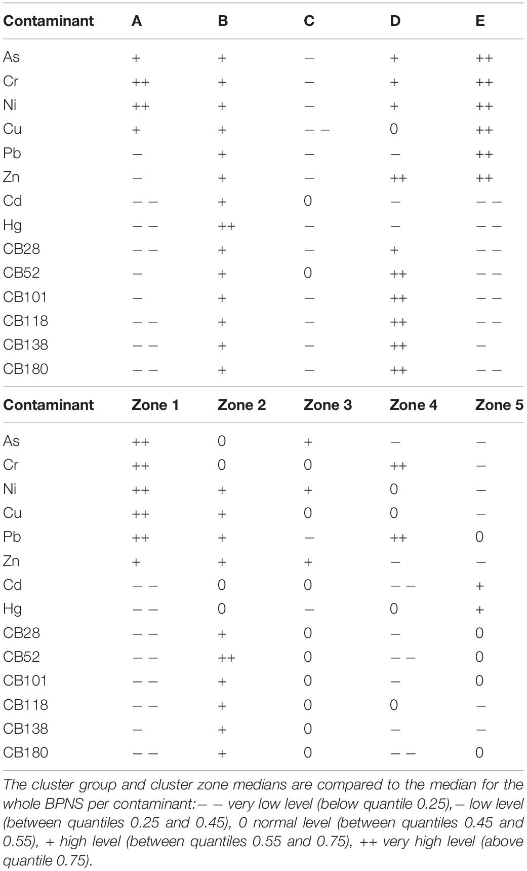
Table 1. Cluster groups (A-E, based on Ward hierarchical clustering) and cluster zone association (zone 1–5, based on cluster groups, PCA and sedimentology characteristics).

FIGURE 5

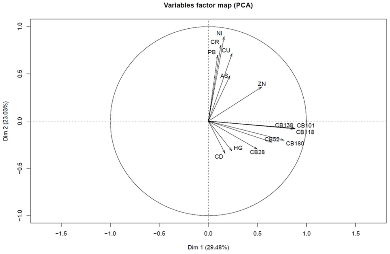
Figure 5. PCA on the subset used for clustering (2007–2011), based on center scaled PCB and metal concentrations (granulometric normalization on the 0–63 μm sediment fraction).

The hierarchical clustering primarily aimed to divide the BPNS into clear spatial zones with specific patterns in contaminant concentrations. As can be seen in Figure 6, the offshore area of the BPNS is dominated by cluster group E (low concentrations in PCBs, Hg, and Cd, and high concentrations of other metals). Therefore we grouped all locations in cluster group E in a more or less clearly distinct offshore Cluster zone 1. This zone is dominated by medium and coarse sands (Hademenos et al., 2018). In the near shore area the cluster groups occurred more mixed, which complicated the division in clear spatial zones. Therefore, a further division in spatial cluster zones is partly arbitrarily and mainly based on the ratio of locations belonging to cluster group A and B, in combination with our knowledge on the hydrodynamic environment and sedimentological characteristics of the BPNS as described by Hademenos et al. (2018). Cluster zone 2 showed a clear dominance of cluster groups B and C and a lack of cluster groups A and E. The area is characterized by fine to medium sands and high concentrations in PCBs and metals (Table 1). Differences between cluster zones 3, 4 (and 5) are rather limited. A mixture of the remaining cluster groups (A, B, C) and to a lesser extent group D (mainly in cluster zone 3) is found. As cluster zone 5 has clearly distinct sedimentology dominated by silt and clay, it was decided to group these locations as a distinct zone. Consequently, cluster zones 3 and 4, which are dominated by fine sand (Hademenos et al., 2018), were automatically delineated, as they are spatially separated in relation to cluster zones 2 and 5. Cluster zones 3, 4 and 5 are characterized by very low to medium PCB concentrations, with low to medium metal concentrations except for Cd and Hg in zone 5, As, Ni and Zn in zone 3 and very clearly for Cr and Pb concentrations in cluster zone 4 (Table 1).

FIGURE 6

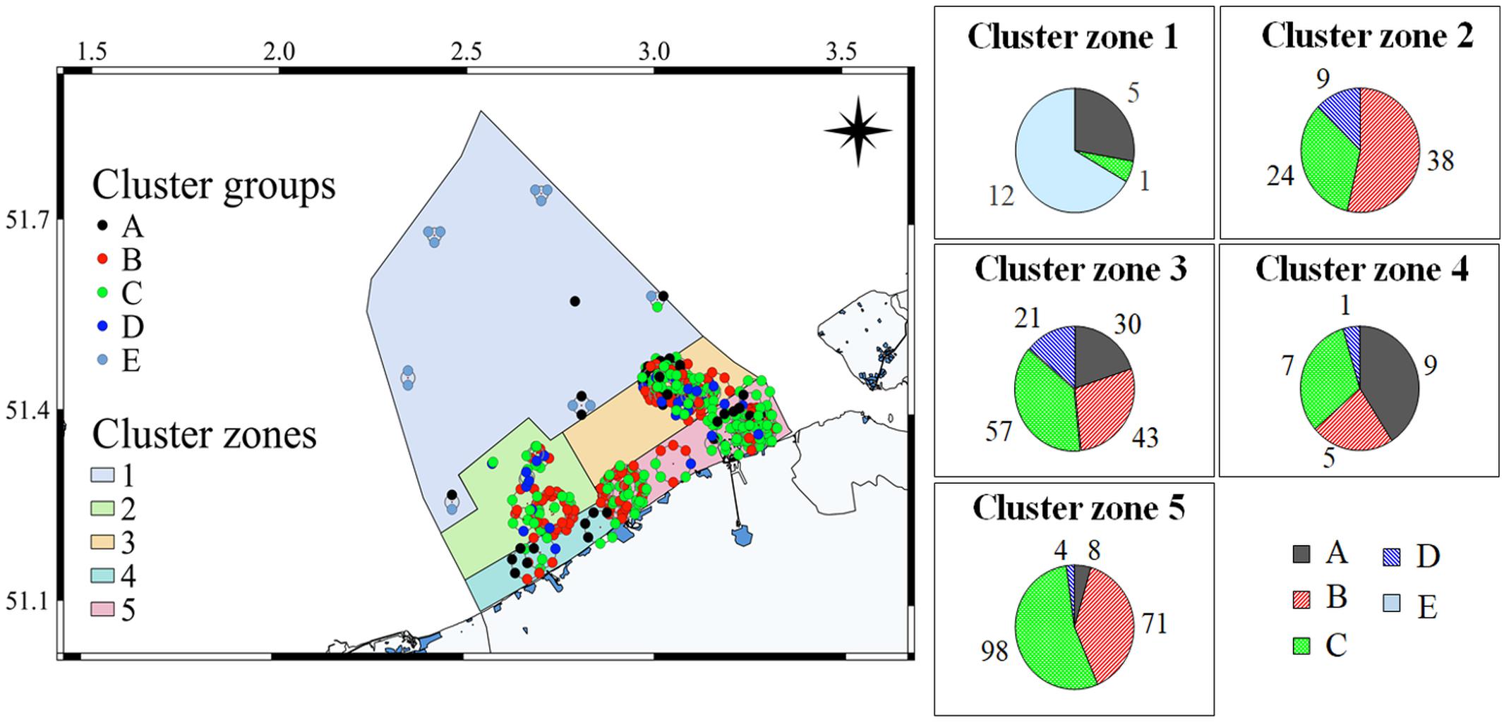
Figure 6. Spatial zonation of the BPNS into five cluster zones, based on Ward hierarchical clustering (cluster groups), the PCA association patterns, and sedimentological characteristics. Numbers in the pie diagrams represent the number of samples/locations found in each cluster group per cluster zone.

Evaluation and Validation of the Normalization Procedures

Co-factor Selection

The best co-factor or normalizer is presented by the highest R² value in the contaminant-co-factor linear relationship. Two examples for Hg vs. Fe and CB153 vs. TOC are given in Figure 7.

FIGURE 7

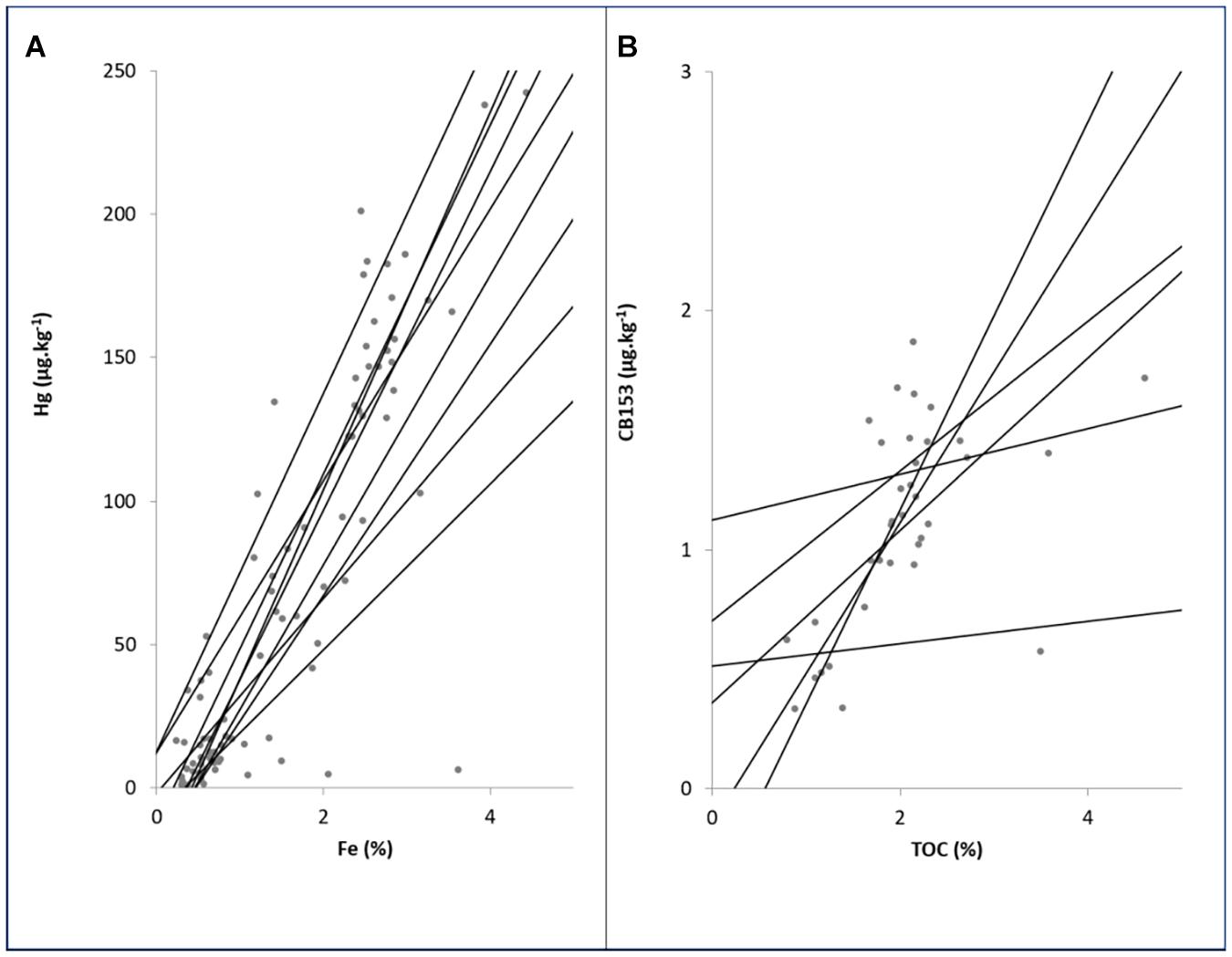
Figure 7. Contaminant—co-factor linear relationships for (A) Hg-Fe and (B) CB153-TOC based on 9 sediment samples collected in March 2015 across the BPNS and fractionated in equally polluted subsamples (9 sediment particle size classes).

Median determination coefficients (median R² values) for the linear regressions between the eight studied metals and the four co-factors (Al, Fe, Ni, and TOC) varied from 0.71 to 0.98, except for As where R² varied from 0.40 and 0.68 (Table 2). Highest R²-values for As, Cd, Ni and Hg were obtained for co-factor TOC. However, the historic datasets collected within the 4DEMON project (period 1971–2015) showed that TOC data are frequently missing. In addition, switches in analytical method over time occurred more often for TOC than for metals. For modeling time trends based on long-term data series such as the 4DEMON dataset, this would increase the number of changes in analytical methods within the normalized dataset, resulting in more complex models. TOC was therefore not withheld for metal normalization in the final modeling approach. On the contrary, metal normalizers are mostly determined by the same analytical method as the contaminant itself, supporting the use of the metal normalization procedures. When comparing the performance of Al with Fe for metal normalization at the BPNS, Fe was found to be a better co-factor than Al for all analyzed contaminants. Interestingly, for all metals except for Cr, linear regressions to Ni revealed higher R² values compared to regressions to Al and Fe as co-factor (Table 2).

TABLE 2

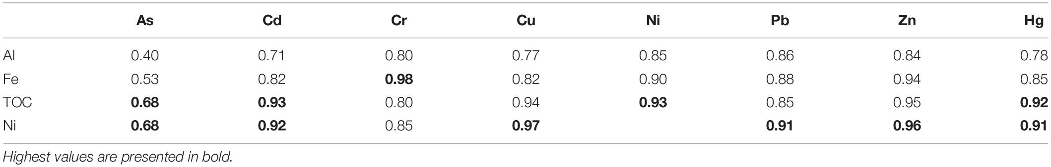
Table 2. Median R² values for the linear regressions between contaminant concentrations (8 metals) and 4 co-factors, based on nine sampling locations (period 2008–2014).

Whereas appropriate co-factors could be found for metals in sediment, surprisingly, the analysis of equally polluted samples resulted in poor results for PCBs against the potential co-factor TOC, with median R² values varying between 0.05 for CB28 and 0.56 for CB101. This is shown in Figure 7B for CB153, where linearity is poor and no clear intercept could be derived from the different regression lines. Since organic contaminants have a strong affinity with organic matter (OSPAR, 2018), a linear relationship was expected. The lack of a linear relationship might be related to low PCB concentrations in the medium and coarse sediment fractions at low TOC values, increasing variability. For trend analysis, it was decided to only consider a granulometric normalization, and limit the PCB time trend modeling to the <63 μm sediment fraction.

Normalization Constants

In addition to the normalizer, also the pivot values Nx, Cx for all metals and the standard seafloor values Nss (for the co-factors corresponding to 2.5% TOC) have to be determined. The values Nx and Cx, derived from pure sand samples (taken offshore BPNS, DS4) are compared with pivot values derived by Smedes et al. (1997) for the neighboring Dutch part of the North Sea, and with the OSPAR values used for metal determination through total digestion methods (OSPAR, 2008; Table 3).

TABLE 3

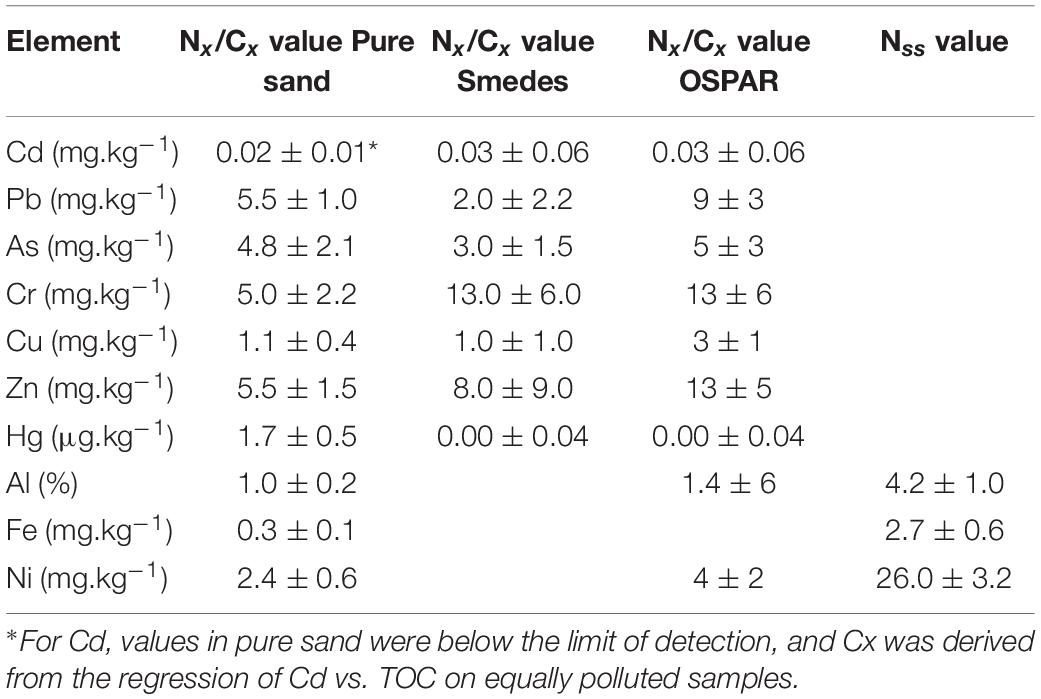
Table 3. Pivot values (Nx/Cx) and standard seafloor concentrations (Nss) with respective standard deviations, and compared to values presented in Smedes et al. (1997) and OSPAR (2008).

The pivot values may have a large impact on the normalization result. Within Eq.2, the denumerator is defined as Ns – Nx. When Ns approaches Nx, large errors can be created due to analytical variations, and when Ns – Nx is <0, normalization is even impossible (OSPAR, 2015). Pivot values are regionally dependent. For example, in the Venice lagoon in northern Italy, Al revealed similar concentrations in coarse and fine fractions due to the presence of feldspars in the coarse fraction (Miserocchi et al., 2000). Al values in sediments from Canadian waters are much higher than in sediments of Dutch marine waters (Smedes et al., 1997). Furthermore, pivot values are dependent on the extraction method. A total digestion method for metal extraction usually results in larger values for Cx and Nx than weak digestion methods (OSPAR, 2015).

Within the 4DEMON project, more than 14,000 metal contaminant values were collected from the main dataset based on four decades of marine monitoring in the BPNS (1971–2015). To minimize normalization errors, we tested the variability between different methods of metal normalization, by calculating the amount of samples with a low denumerator in the main dataset. Normalization to Al with the selected pure sand pivot values resulted in 8.2% of all contaminant values with Ns-Nx <0 and 9.3% with Ns-Nx <1. With Fe normalization, the amount of contaminant values with Ns-Nx <0 and <1 was 3.3 and 13.5%, respectively.

Validation of the Geochemical Normalization Procedures

For metals, the geochemical normalization methods hybrid 1, hybrid 2, and Ni were compared to the normalization procedure to Al and to Fe independently, using the equally polluted sample set (sampled at nine locations across the BPNS in March 2015). Results are presented in Table 4 as relative values (%) compared to the lowest (best) values for a given metal for the interquartile range (IQR) score and the difference between mean and median, respectively. Also, absolute values for outlier score and number of discarded values have been calculated.

TABLE 4

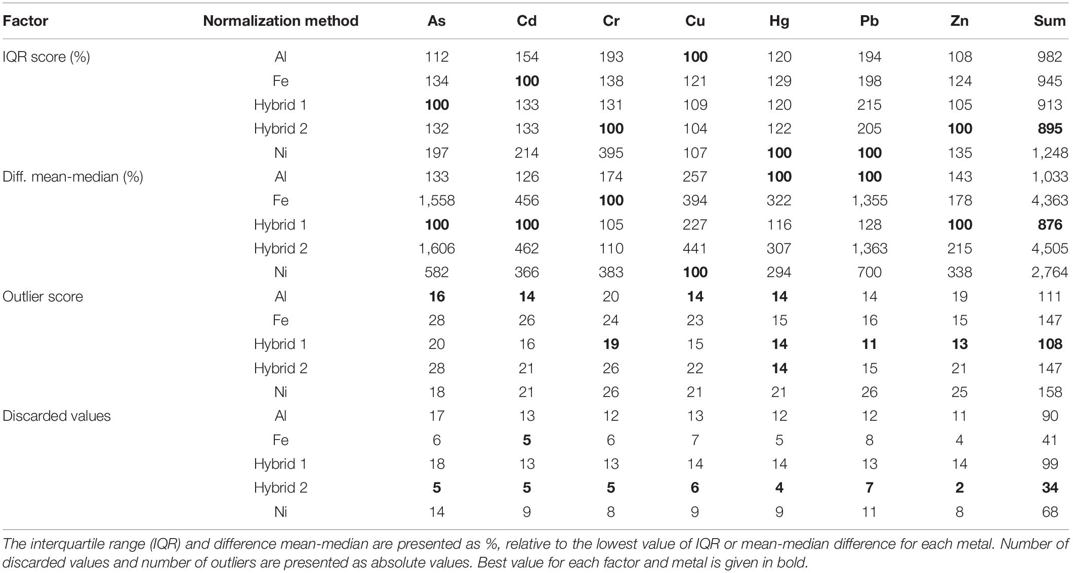
Table 4. Variability performance of the five normalization methods.

The choice for the best normalizer is a weighing between different factors. Reduced variability, expressed by a low IQR score and a small difference between mean and median, can be expected to be linked to a higher number of discarded values. Normalization method hybrid 1, closely followed by normalization to Al, resulted in low differences between mean and median and low interquartile ranges (IQR) (Table 4). Hybrid 1 provided best reliable normalized values, however, the resulting final dataset size was largely reduced due to the deviation range condition, leading to the highest number of discarded values. By applying hybrid method 1, 13–18 values (on a total of 82 for each metal) from the equally polluted samples dataset were discarded (comparable to the number discarded when using the Al normalization procedure). Discarding these values also led to a relatively low number of remaining outliers for all metals, varying from 11 to 20, which will reduce data variation when this normalization method is applied within time series analysis.

On the other hand, hybrid 2 and Fe normalization equally resulted in low IQR scores, but showed higher numbers of outliers and larger differences between mean and medium (Table 4). This is especially true for As and Pb. In contrast, the number of discarded values (2–7) was much lower for the individual metals in both hybrid 2 and Fe normalization procedures. Within the 4Demon dataset, the measured contaminant concentration normalized to Al (N_S,AL) was lower than the contaminant pivot value normalized to Al (N_X,AL) for 8.2% of the metal values. Within normalization method hybrid 2, most of these values are not discarded as the hybrid 2 procedure then returns a value normalized to Fe. This leads to a higher amount of low concentration values within hybrid 2 compared to hybrid 1. This enlarged the variability of the normalized values distribution, which is in particular apparent by the introduction of a higher amount of outliers, but did not affect the interquartile range.

Ni proved to be the best co-factor for BPNS sediment contaminant normalization based on the contaminant-cofactor linear regressions (Table 2). However, Ni normalization resulted in relatively higher interquartile ranges and the highest number of outliers compared to the other normalization approaches (Table 4).

With the objective of limiting the exclusion or downsizing older data, which is often the case when using data based on total sediment analyses with unknown measurement uncertainty, the proposed normalization procedures are believed to have a substantial added value compared to for example the OSPAR protocol (OSPAR, 2018). The methods counter the risk of errors created by normalizer values close to Nx. Moreover, the selected normalizers have been routinely analyzed within marine monitoring and research programs in the BPNS over the past decades, with Ni values available since 1971 and Fe and Al values available since 1979. This makes them perfectly suitable to be applied on long-term datasets. The ultimate choice depends on the project goals and the metadata availability.

Long-Term Trend Analyses on the BPNS Based on Linear Mixed Effect Modeling

Trends and spatial differences in PCBs and metal contamination in the BPNS have been deduced from linear mixed-effects models, built on four decades of PCB concentrations (<63 μm sediment fraction) and eight metal concentrations normalized with four normalization procedures, granulometric (<63 μm fraction), Hybrid 1 and 2 (as combinations of Al and Fe), and Ni normalization. Detailed results of all models, with data counts, removed outliers, information on each model parameter, and trend graphs are provided as Supplementary Figures 2–9 and Supplementary Table 2). A selection of trend graphs is presented in Figures 8–10.

FIGURE 8

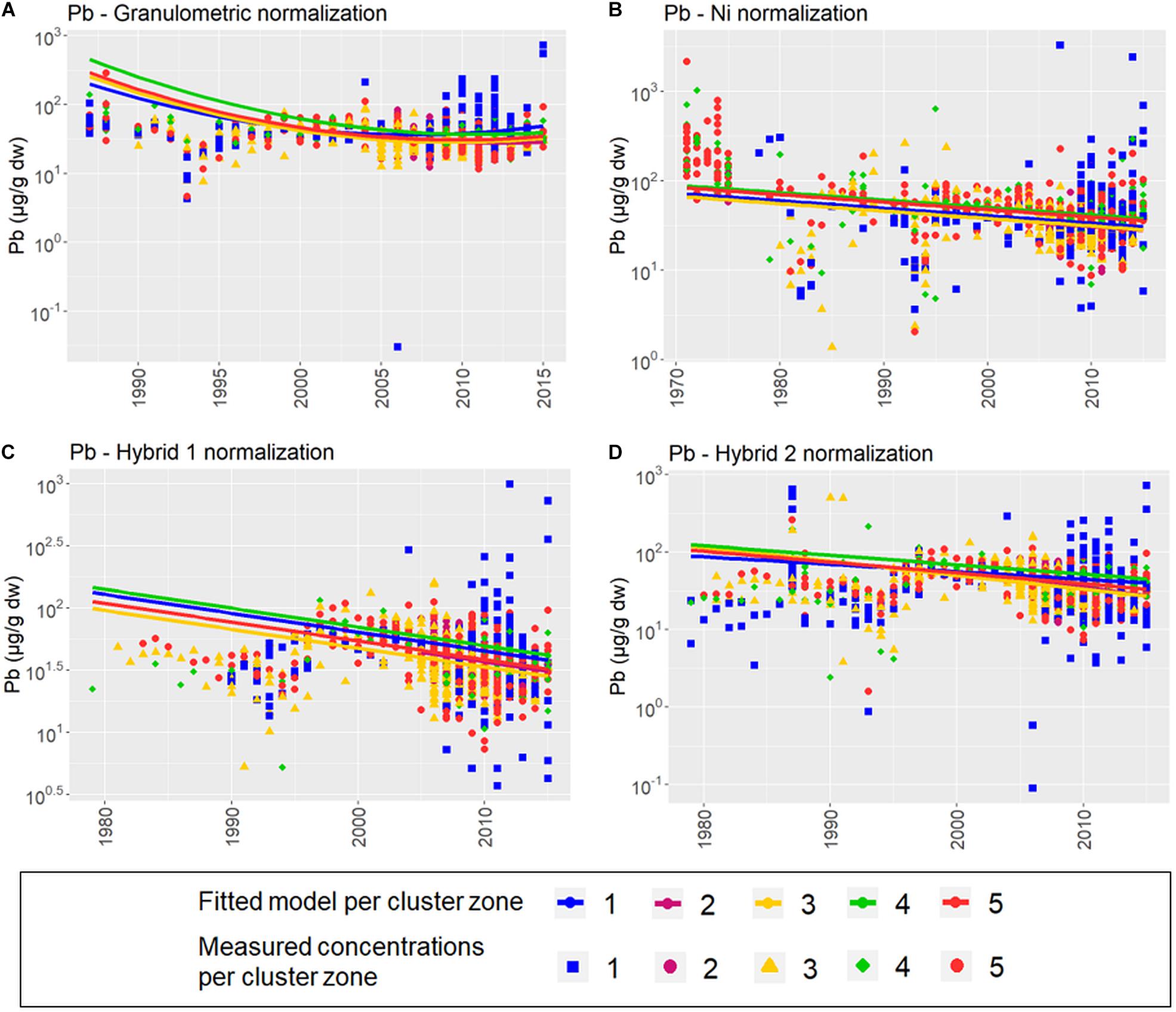
Figure 8. Trends in log Pb in sediments of the BPNS, applying (A) granulometric normalization (<63 μm, 1987–2015), (B) Ni normalization (1971–2015), (C) Hybrid method 1 (1979–2015) and (D) Hybrid method 2 (1979–2015). Data points represent the derived concentrations, after normalization. Colored regression lines represent the fitted time trends within each spatial cluster zone, scaled to the first quadrimester and to the most recent analytical method.

Modeling of Metal Data

The change in log transformed metal concentrations is presented in Table 5 for the entire modeled period as well as for the last 5 years of the model. Time trends for Pb for the different normalization methods are presented in Figure 8. Modeling start date depends on the selected normalization method, with longest time trends starting in 1971 for Ni normalization. As analytical method is a model parameter, data point shifts can be observed. As such, an optical misleading effect may appear that trend lines do not seem to fit all data points. E.g., a constant decrease in Pb concentrations can be seen in the data of the eighties and first half of the nineties in Figure 8C, followed by a steep increase in concentrations in 1996–1997, again followed by a constant decrease. The instant increase in 1996–1997 is due to a change in instrumentation, as metal detection by graphite furnace atomic absorption spectroscopy was changed to inductively coupled plasma-optical emission spectrometry in that period, and significantly increased the recorded Pb values.

TABLE 5

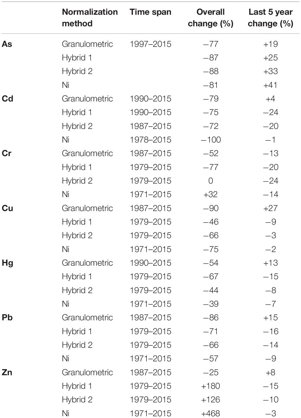
Table 5. Overall trend (% increase or decrease) in metal concentrations over the total time series and over the last 5 years of the modeled time period (2011–2015) for each normalization method.

Although hybrid 1 normalization showed a reduced variability by discarding a higher amount of values (10.6% on a time series of 1,373 data points) compared to hybrid 2 and Ni normalization, this did not affect the overall Pb time trend, with a total overall reduction of 71% compared to 66 and 57%, respectively (Table 5 and Figure 8). Results of the granulometric normalization showed the same trend, be it on a shorter time scale (86% overall reduction). For As, Cu, Cd, and Hg, the differences between normalization methods were limited, with metal reductions over the total time span (1971–2015) varying from 39% (Hg, Ni normalization) to 100% (Cd, Ni normalization) (Table 5). As can be seen for Pb (Figure 8) or for other metals (Figure 9; Supplementary Figures 2–8), the strong metal reduction in all zones of the BPNS can be seen as a result of a linear decrease or a strong decrease over the first decades followed by a steady state or slight increase since 2010–2011 (Table 5). Only for Cr (and Zn, see further), the outcomes of the normalization procedures differed: granulometric normalization and hybrid 1 revealed a decrease, while hybrid 2 and Ni normalization showed a steady state or even a small increase (Table 5 and Supplementary Figure 3). The models for Cr differed especially in the first decades of the considered time frame, while all models showed a decrease since 2000.

FIGURE 9

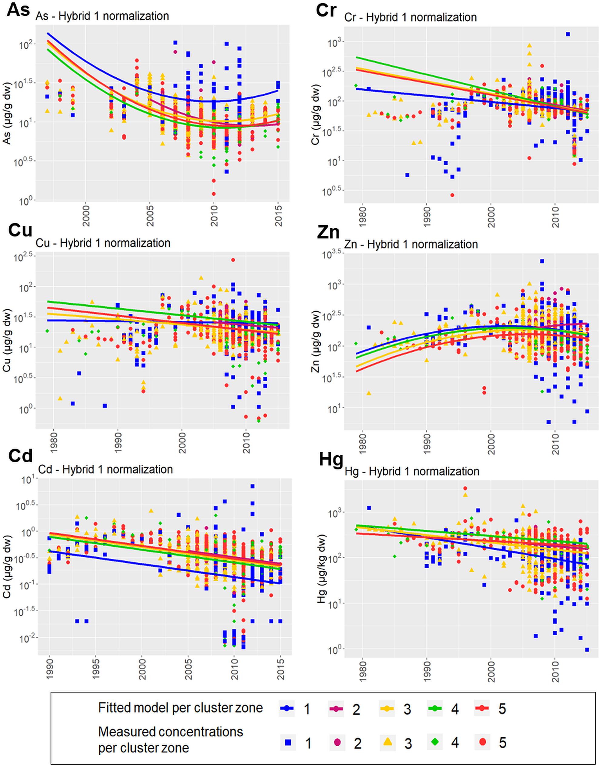
Figure 9. Trends in metals in the BPNS based on Hybrid normalization method 1. Data points represent the derived concentrations after normalization. Colored regression lines represent the fitted time trends within each spatial cluster zone, scaled to the first quadrimester and to the most recent analytical method.

When differences in cluster zones are studied in more detail, it can be seen that the more offshore cluster zone 1, had higher normalized As concentrations. Also, consistent with the cluster analyses based on the 5 years’ subset, Hg and Cd presented lower concentrations at spatial cluster zone 1. The observed decrease for Pb and most other metals were as expected, related to pollution control measures at industrial combustion processes and metal production, transport and waste streams (OSPAR, 2010). Moreover, the observed time trends are in line with other published time trends on metals in the BPNS or the North Sea. Guns et al. (1995) evaluated the period 1979–1995, Gao et al. (2013) looked at 1978–1998, and De Witte et al. (2016) covered the period 2005–2014. Also, decreasing metal time trends were noted in the OSPAR assessment for 1998–2007 in the North-East Atlantic, which includes the North Sea (OSPAR, 2010). In the OSPAR intermediate assessment covering period 2005–2015 (OSPAR, 2017), a decrease in Hg concentrations was noted but no statistical changes occurred for Cd and Pb during that period in the southern part of the North Sea. These results proof that the applied trend models for Pb are robust for the normalization selection and in line with international assessments within the same region. The inclusion of historical data from the nineteen seventies and eighties hampered the use of highly qualitative and standardized OSPAR procedures for data assessment on the entire 4Demon data set. The integration of various analytical methods from different data owners as well as the spatial clustering of locations induces variability. In contrast to the OSPAR procedure, data with larger measurement uncertainty was not excluded or downsized, since this would have eliminated especially the oldest data, often measured on the whole sediment fraction. To ensure a qualitative assessment, alternative quality checks were introduced at the stage of the normalization and by applying an outlier test. The similarity of trends compared to international standardized procedures shows the robustness of the applied methodology.

In contrast to the other metals, Zn models with the three geochemical normalization procedures (period 1971 or 1979–2015) showed a general increase between 126% (hybrid 2) and 468% (Ni normalization). Only granulometric normalization showed a limited decrease (−25%) on a shorter timeframe (1987–2015). At specific locations in the BPNS and on a limited timeframe (2005–2014), a Zn increase was already noted by De Witte et al. (2016) in cluster zone 2 (sludge disposal site Nieuwpoort) and at the west side of cluster zone 5 (nearby sludge disposal site Oostende). The present study confirms that also on a larger time frame and within the different cluster zones of the BPNS, trends in Zn concentrations are increasing. Zn is a metal with multiple sources in the marine environment. Between 1961 and 1985, huge amounts of Zn were dumped at the BPNS originating from titanium dioxide industrial waste. On average 600,000 tons of waste was discharged yearly within this period, containing 120,000 tons of sulphuric acid but also 3 tons of Zn (Baeteman et al., 1987). Next to Cu, Zn is also used in marine antifouling products, especially since the ban on TBT in antifouling paints (Turner, 2010), and as anode on ships and marine constructions, like windmill parks (Kirchgeorg et al., 2018). Moreover, Zn is identified as an important contaminant within the adjacent river Scheldt, which connects the port of Antwerp with the BPNS, and is therefore put forward as a pollutant to be monitored in the coastal zone of the BPNS within the Water Framework Directive (Belgische Staat, 2016). Considering the expansion of windmill parks at the BPNS, combined with increasing trends in shipping traffic, it will be of special interest to follow up Zn concentrations in the upcoming years.

Modeling of PCB Data

PCBs revealed a decreasing trend from 1991 to 2015 in marine sediments of the BPNS (Figure 10), with a total change, averaged over the five spatial cluster zones, varying from −36% for CB118 to −60% for CB180 (see Supplementary Figure 9). The overall decrease for most PCBs resulted from a strong decrease in the nineties, followed by a leveling off or even an increase over the last 10–15 years. The offshore spatial cluster zone 1 showed the most intense decrease for all PCB congeners, from −18% overall reduction for CB52 to −89% for CB101, leading to the lowest contamination levels in spatial cluster zone 1 in the most recent years (2010–2015) compared to the other cluster zones. This is consistent with the low levels which were already seen in the cluster analyses (period 2008–2014). Spatial cluster zones 3 and 5 showed the lowest decrease, with even an overall increase for CB28, CB52 and CB118 at cluster zone 5.

FIGURE 10

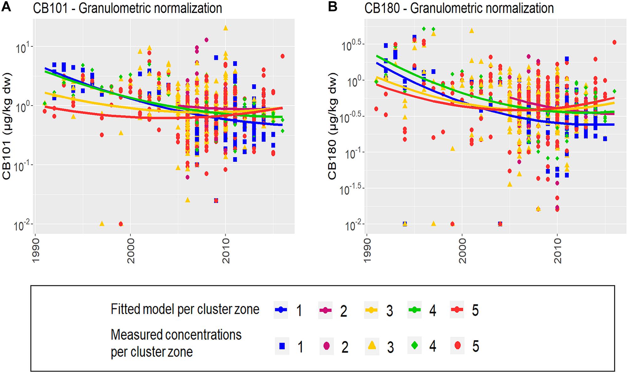
Figure 10. Trends in PCBs in sediments of the BPNS based on granulometric normalization (<63 μm sediment fraction). (A) CB101, (B) CB180. Colored regression lines represent the fitted time trends within each cluster zone, scaled to the first quadrimester and to the most recent analytical method.

For PCB trends in sediment of the BPNS and the southern part of the North Sea, contradictory information is found in literature. Roose et al. (2005) did not find a significant decrease from 1991 to 2001 for CB153 in sediments. The OSPAR quality status report (OSPAR, 2010) indicated no significant decrease for more than 80% of the PCB time series (1998–2010) in the North Sea whereas a downward trend was modeled for the Southern North Sea between 1995 and 2015 (OSPAR, 2017). De Witte et al. (2016) recorded a steady state or even an increase in PCB concentrations from 2005 to 2014. In contrast, Everaert et al. (2014) found a 50–66% decrease from 1991 to 2010. With the advantage of considering a larger timeframe and taking into account method switches within the 4DEMON dataset, our results proved to be consistent with all mentioned publications, as the modeled trend analyses showed a strong decrease in PCB concentrations in the BPNS, followed by a steady state or increase. The lower reductions and higher levels in PCB concentrations in cluster zones 3 and 5 compared to the offshore cluster zone 1, can be related to inputs from the nearby port of Zeebrugge and the Scheldt estuary. Everaert et al. (2014) found no PCB decrease between 1991 and 2010 in the Scheldt sediments. Continuous inputs of suspended solids from the Scheldt estuary into BPNS cluster zones 3 and 5 might affect PCB trends in these nearshore areas.

Conclusion

The aim of this study was to develop extended, multi-decade trends on metals and PCBs in the marine environment, based on different monitoring and research studies in the BPNS. Multi-decade trend analysis might provide valuable information within a broad perspective for scientists and policymakers on anthropogenic impacts on the marine environment. However, the integration of historical data from the nineteen seventies and eighties into long-term time trends implied some major issues to be solved: sampling locations changed over time, different analytical methods were applied, analyses were performed on different grain size fractions and not all appropriate normalizers were analyzed for all samples. These limitations hampered the use of the highly qualitative and standardized OSPAR protocols. Alternative approaches were developed and applied, so that the oldest historical samples, which are often measured on the whole sediment fraction and contain less metadata amongst which information on measurement uncertainty, can be retained for the modeling approach. This works presents a novel approach, where spatial clustering is combined with different adapted normalization methods and integrated in long-term trend parametric linear mixed effect models. This novel approach was used to integrate different valuable PCB and metal datasets gathered between 1971 and 2015 in the BPNS.

Project results revealed major differences in metal distribution, with relatively high Cd and Hg concentrations at the coastal zone where the sediment clay fraction is high. Model results also revealed increasing Zn concentrations for 3 out of 4 normalized models, while PCB concentrations are slightly increasing in the BPNS over the last decade (2005–2015). Local increases of Zn and PCB stress the importance of continuous monitoring, even of banned substances. This study also showed the importance of compiling real long-term trends: different publications on PCBs in sediments of the BPNS came to different trend conclusions depending on the time period studied; our overarching assessment provides a broader perspective, complementing and completing the results of the shorter time trend studies.

The applied clustering, normalization and modeling approaches may be of high value for multi-decade contaminant time trend analyses in other geographical regions. Of course, case dependent differences will remain; if datasets are too fragmented, with many data originators and multiple method changes, trend modeling might be hampered. Moreover, the selection of appropriate co-factors is dependent on the available metadata within each dataset and the normalization constants are dependent on region and analytical method. Still, we believe we proved the added value of this combined approach to analyze long term trends in four decades of metal and PCB contamination data.

Data Availability Statement

The datasets presented in this study can be found in online repositories. The names of the repository/repositories and accession number(s) can be found below: 4DEMON, 2020. 4DEMON: 4 decades of metals and PCBs concentrations in sediment at the Belgian Part of the North Sea. Dataset. doi.org/10.24417/bmdc.be:dataset:2400.

Author Contributions

HL: data collection, data analysis, and writing. KB: data collection, data analysis, and review. RL: data collection, project coordinator, and review. BA: data analysis and review (main expertise input: statistics). AR: review (main expertise input: metal data analysis). KD: review (main expertise input: organics data analysis). KH: writing and review (main expertise input: statistics and overall data analysis). BD: data collection, data analysis, writing, and review. All authors have a substantial contribution to this publication with respect to data collection, data analysis and writing and approve the final version of the manuscript.

Funding

The4DEMON project was financed by Belspo (project no. BR/121/A3/4DEMON).

Conflict of Interest

The authors declare that the research was conducted in the absence of any commercial or financial relationships that could be construed as a potential conflict of interest.

Acknowledgments

We acknowledge all scientists and co-workers within the projects “Projet Mer/Project Zee,” the “Monitoring Master Plan for the North Sea, the monitoring of sludge disposal and sand extraction, the Ph.D. of Dr. Veerle Van Alsenoy, the co-workers of OD Nature, Sciensano and ILVO contributing to both OSPAR and MSFD monitoring and the Ecochem Laboratory of Dr. Koen Parmentier for the use of the siever. Monitoring and research data were obtained aboard the vessels Paster Pijpe, RV Belgica (operated by the Belgian Navy under charter of RBINS), Last Freedom, Stream, and RV Simon Stevin (VLIZ). The part on normalization methods was submitted earlier as separate publication, but based on the reviewers comments, reformatted, adapted and extended with the real time trend assessments.

Supplementary Material

The Supplementary Material for this article can be found online at: https://www.frontiersin.org/articles/10.3389/fmars.2021.681901/full#supplementary-material

References

4DEMON (2020). 4DEMON: 4 decades of metals and PCBs concentrations in sediment at the Belgian Part of the North Sea. Dataset doi: 10.24417/bmdc.be:dataset:2400

CrossRef Full Text | Google Scholar

Assefa, A. T., Sobek, A., Sundqvist, K. L., Cato, I., Jonsson, P., Tysklind, M., et al. (2014). Temporal trends of PCDD/Fs in Baltic Sea sediment cores covering the 20th Century. Environ. Sci. Technol. 48, 947–953. doi: 10.1021/es404599z

PubMed Abstract | CrossRef Full Text | Google Scholar

Baeteman, M., Vyncke, W., Gabriels, R., and Guns, M. (1987). Heavy Metals in Water, Sediments and Biota in Dumping Areas for Acid wastes from the Titanium Dioxide Industry. Copenhagen: Internatinoal Council for the Exploration of the Sea.

Google Scholar

Bates, D., Maechler, M., Bolker, B., and Walker, S. (2015). Fitting linear mixed-effects models using lme4. J. Stat. Softw. 67, 1–48. doi: 10.18637/jss.v067.i01

CrossRef Full Text | Google Scholar

Belgische Staat (2016). Stroomgebiedsbeheersplan voor de Belgische kustwateren voor de implementatie van de Europese Kaderrichtlijn Water (2000/60/EG) voor de periode 2016-2021. Brussels: Federale Overheid van België, 96.

Google Scholar

Cundy, A. B., Croudace, J. W., Cearreta, A., and Irabien, M. J. (2003). Reconstructing historical trends in metal input in heavily-distrubed, contaminated estuaries : studies from Bilbao, Southampton Water and Sicily. Appl. Geochem. 18, 311–325. doi: 10.1016/S0883-2927(02)00127-0

CrossRef Full Text | Google Scholar

De Witte, B., Ruttens, A., Ampe, B., Waegeneers, N., Gauquie, J., Devriese, L., et al. (2016). Chemical analyses of dredged spoil disposal sites at the Belgian part of the North Sea. Chemosphere 156, 172–180. doi: 10.1016/j.chemosphere.2016.04.124

PubMed Abstract | CrossRef Full Text | Google Scholar

Everaert, G., De Laender, F., Deneudt, K., Roose, P., Mees, J., Goethals, P. L. M., et al. (2014). Additive modelling reveals spatiotemporal PCBs trends in marine sediments. Mar. Pollut. Bull. 79, 47–53. doi: 10.1016/j.marpolbul.2014.01.002

PubMed Abstract | CrossRef Full Text | Google Scholar

Everaert, G., Ruus, A., Hjermann, D. Ø, Borga, K., Green, N., Boitsov, S., et al. (2017). Additive models reveal sources of metals and organic pollutants in Norwegian marine sediments. Environ. Sci. Technol. 51, 12764–12773. doi: 10.1021/acs.est.7b02964

PubMed Abstract | CrossRef Full Text | Google Scholar

Fettweis, M., Houziaux, J.-S., Du Four, I., Van Lancker, V., Baeteman, C., Mathys, M., et al. (2009). Long-term influence of maritime access works on the distribution of cohesive sediments: analysis of historical and recent data from the Belgian nearshore area (southern North Sea). Geo Mar. Lett. 29, 321–330. doi: 10.1007/s00367-009-0161-7

CrossRef Full Text | Google Scholar

Folk, R. L. (1954). The distinction between grain size and mineral composition in sedimentary rock nomenclature. J. Geol. 62, 344–359. doi: 10.1086/626171

CrossRef Full Text | Google Scholar

Gao, Y., De Brauwere, A., Elskens, M., Croes, K., Baeyens, W., and Leermakers, M. (2013). Evolution of trace metal and organic pollutant concentrations in the Scheldt River Basin and the Belgian Coastal Zone over the last three decades. J. Mar. Syst. 128, 52–61. doi: 10.1016/j.marsys.2012.04.002

CrossRef Full Text | Google Scholar

Grant, A., and Middleton, R. (1998). Contaminants in sediments: using robust regression for grain-size normalization. Estuaries 21, 197–203. doi: 10.2307/1352468

CrossRef Full Text | Google Scholar

Guns, M., Van Hoeywegen, P., Baeten, H., Hoenig, M., Vyncke, W., and Hillewaert, H. (1995). Evolutie van de gehalten van zware metalen in sedimenten van het Belgisch Continentaal Plat (1979-1995). Mededelingen van het Rijksstation voor Zeevisserij, CLO Gent, publicatie nr. 242, D/1997/0889/1.

Google Scholar

Hademenos, V., Stafleu, J., Missaen, T., Kint, L., and Van Lancker, V. R. M. (2018). 3D subsurface characterisaiton of the Belgian continental shelf: a new voxel modelling approach. Net. J. Geosci. 98:e1. doi: 10.1017/njg.2018.18

CrossRef Full Text | Google Scholar

Herut, B., and Sandler, A. (2006). Normalization Methods for Pollutants in Marine Sediments: Review and Recommendations for the Mediterranean. IOLR Report H18/2006. Nairobi: United Nations Environment Programme, 23.

Google Scholar

Kirchgeorg, T., Weinberg, I., Hörnig, M., Baier, R., Schmid, M. J., and Brockmeyer, B. (2018). Emissions from corrosion protection systems of offshore wind farms: evaluation of the potential impact on the marine environment. Mar. Pollut. Bull. 136, 257–268. doi: 10.1016/j.marpolbul.2018.08.058

PubMed Abstract | CrossRef Full Text | Google Scholar

Lagring, R., Bekaert, K., Borges, A. V., Desmit, X., De Witte, B., Le, H. M., et al. (2018). 4 Decades of Belgian Marine Monitoring: Uplifting Historical Data to Today’s Needs, Final Report. Brussels: Belgian Science Policy, BRAIN-be.

Google Scholar

Lê, S., Josse, J., and Husson, F. (2008). FactoMineR: an R package for multivariate analysis. J. Stat. Softw. 25, 1–18. doi: 10.18637/jss.v025.i01

CrossRef Full Text | Google Scholar

Loring, D. H. (1991). Normalization of heavy-metal data from estuarine and coastal sediments. ICES J. Mar. Sci. 48, 101–115. doi: 10.1093/icesjms/48.1.101

CrossRef Full Text | Google Scholar

Mil-Homens, M., Stevens, R. L., Cato, I., and Abrantes, F. (2014). Comparing spatial and temporal changes in metal trends (Cr, Ni, Pb, Zn) on the Portuguese shelf since the 1970s. Environ. Monit. Assess. 186, 6327–6340. doi: 10.1007/s10661-014-3857-8

PubMed Abstract | CrossRef Full Text | Google Scholar

Miserocchi, S., Bellucci, L. G., Marcaccio, M., Matteucci, G., Landuzzi, V., Quarantotto, G., et al. (2000). Sediment composition and normalisation procedures : an example from a QUASH project sediment exercise. J. Environ Monit. 2, 529–533. doi: 10.1039/B002760J

PubMed Abstract | CrossRef Full Text | Google Scholar

OSPAR (2008). CEMP assessment manual. Co-ordinated Environmental Monitoring Programme Assessment Manual for Contaminants in Sediment and Biota. Monitoring and Assessment Series. London: OSPAR commission, 31.

Google Scholar

OSPAR (2009). Agreement on CEMP Assessment Criteria for the QSR 2010, Agreement Number 2009-2. London: OSPAR commission, 7.

Google Scholar

OSPAR (2010). Quality Status Report 2010. London: OSPAR commission, 176.

Google Scholar

OSPAR (2015). JAMP Guidelines for Monitoring Contaminants in Sediment, Revision 2015. London: OSPAR commission, 111.

Google Scholar

OSPAR (2017). Intermediate Assessment 2017. London: OSPAR commission.

Google Scholar

OSPAR (2018). JAMP Guidelines for Monitoring Contaminants in Sediments. Ospar Commission, Monitoring Guidelines, OSPAR Agreement 2002-16, Update 2018. London: OSPAR commission.

Google Scholar

OSPAR. (2019). OSPAR Coordinated Environmental Monitoring Programme (CEMP). OSPAR Commission, OSPAR Agreement 2016-01, update 2019. London: OSPAR commission.

Google Scholar

Pinheiro, J., Bates, D., Debroy, S., Sarkar, D., and R Core Team (2018). _nlme: Linear and Nonlinear Mixed Effects Models_. R package version 3.1-137.

Google Scholar

R Core Team (2018). R: a Language and Environment for Statistical Computing. Vienna: R foundation for statistical computing.

Google Scholar

Rees, H. L., Eggleton, J. D., Rachor, E., and Vandn Berghe, E. (2007). Structure and Dynamics of the North Sea Benthos. ICES Cooperative Research Report 288. Copenhagen: ICES, 258.

Google Scholar

Roose, P., Raemaekers, M., Cooreman, K., and Brinkman, U. A. T. (2005). Polychlorinated biphenyls in marine sediments from the southern North Sea and Scheldt estuary: a ten-year study of concentrations, patterns and trends. J. Environ. Monit. 7, 701–709. doi: 10.1039/b419240k

PubMed Abstract | CrossRef Full Text | Google Scholar

Smedes, F., Lourens, J., and van Wezel, A. (1997). Zand, slib en zeven: standaardisering van contaminantgehaltes in mariene sedimenten. Rapport RIKZ-96.043. The Hague: Rijksinstituut voor Kust en Zee\RIKZ, 135.

Google Scholar

Smedes, F., and Nummerdor, G. A. N. (2003). Grain-Size Correction for the Contents of Butyltin Compounds in Sediment. Report RIKZ\2003.035. The Hague: National Institute of coastal and marine management\RIKZ, 40.

Google Scholar

Sobek, A., Sundqvist, K. L., Assefa, A. T., and Wiberg, K. (2015). Baltic Sea sediment records: unlikely near-future declines in PCBs and HCB. Sci. Total Environ. 518-519, 8–15. doi: 10.1016/j.scitotenv.2015.02.093

PubMed Abstract | CrossRef Full Text | Google Scholar

Traven, L. (2013). Sources, trends and ecotoxicological risks of PAH pollution in surface sediments from the northern Adriatic Sea (Croatia). Mar. Pollut. Bull. 77, 445–450. doi: 10.1016/j.marpolbul.2013.08.043

PubMed Abstract | CrossRef Full Text | Google Scholar

Turner, A. (2010). Marine pollution from antifouling paint particles. Mar. Pollut. Bull. 60, 159–171. doi: 10.1016/J.marpolbul.2009.12.004

PubMed Abstract | CrossRef Full Text | Google Scholar

Van Alsenoy, V. (1993). Concentration and Partitioning of Heavy Metals in the Scheldt estuary. Ph. D. thesis. Antwerp: Antwerp University, 290.

Google Scholar

Wafo, E., Abou, L., Nicolay, A., Boissery, P., Pereze, T., Abondo, R. N., et al. (2016). A chronicle of the changes undergone by a maritime territory, the Bay of Toulon (Var Coast, France) and their consequences on PCB contamination. Springerplus 5:1230. doi: 10.1186/s40064-016-2715-2

PubMed Abstract | CrossRef Full Text | Google Scholar

Ward, J. H. Jr. (1963). Hierarchical grouping to optimize an objective function. J. Am. Stat. Assoc. 58, 236–244. doi: 10.1080/01621459.1963.10500845

CrossRef Full Text | Google Scholar

West, J. E., O’Neil, S. M., and Ylitalo, G. M. (2017). Time trends of persistent organic pollutants in benthic and pelagic indicator fishes from Puget Sound, Washington, USA. Arch. Environ. Contam. Toxicol. 73, 207–229. doi: 10.1007/s00244-017-0383-z

PubMed Abstract | CrossRef Full Text | Google Scholar

Yake, B. (2001). The Use of Sediment Cores to Track Persistent Pollutants in Washington State: A Review. Lacey, WA: Washington State Department of Ecology.

Google Scholar

Zuur, A. F., Ieno, E. N., Walker, N. J., Saveliev-Graham, A. A., and Smith, M. (2009). Mixed Effects Models and Extensions in Ecology with R. New York, NY: Springer, 580.

Google Scholar