Mechanisms of Lateral Spreading in a Near-Field Buoyant River Plume Entering a Fjord

Observations collected from a fast-flowing buoyant river plume entering the head of Doubtful Sound, New Zealand, were analysed to examine the drivers of plume lateral spreading. The near-field plume is characterised by flow speeds of over 2 ms⁻¹, and strong stratification (N² > 0.1 s⁻²), resulting in enhanced shear which supports the elevated turbulence dissipation rates (ϵ > 10⁻³ W kg⁻¹). Estimates of plume lateral spreading rates were derived from the trajectories of Lagrangian GPS surface drifters and from cross-plume hydrographic transects. Lateral spreading rates derived from the latter compared favourably with estimates derived from a control volume technique in a previous study. The lateral spreading of the plume was driven by a baroclinic pressure gradient toward the base of the plume. However, spreading rates were underestimated by the surface drifters. A convergence of near-surface flow from the barotropic pressure gradient concentrated the drifters within the plume core. The combination of enhanced internal turbulence stress and mixing at the base of the surface layer, and the presence of steep fjord sidewalls likely reduced the rate of lateral spreading relative to the theoretical spreading rate. The estimates of plume width from the observations provided evidence of scale-dependent dispersion which followed a 4/3 power law. Two theoretical models of dispersion, turbulence and shear flow dispersion, were examined to assess which was capable of representing the observed spreading. An analytical horizontal shear-flow dispersion model generated estimates of lateral dispersion that were consistent with the observed 4/3 law of dispersion. Therefore, horizontal shear dispersion appeared to be the dominant mechanism of dispersion, thus spreading, in the surface plume layer.

1. Introduction

Buoyant river plumes inject large freshwater discharges and terrigenous material into the coastal ocean. Such input, particularly sediment, pollutants and nutrients, can have significant environmental implications. For example, the high nutrient content of water runoff from agricultural lands can cause algal blooms, with adverse effects on marine life (Durand et al., 2002). Similarly, treated wastewater is often discharged into adjacent waters which leads to residual nutrient and contaminant loading (Roberts, 1999; Hunt et al., 2010). Accurate predictions of the ultimate fate and impact of the riverine waters and related material require an understanding of the plume dynamics over a broad range of spatial scales, typically considered in terms of near and far-field processes.

The near-field region, immediately seawards of the plume discharge point, is where the momentum-dominated initial river discharge transitions into a buoyancy-forced plume. The dynamics in this near-field region are governed by turbulent mixing, driven by the initial momentum anomaly which enhances velocity shear, and lateral spreading (Hetland, 2005, 2010). The mid-field region occurs after the inflow momentum is depleted by these near-field processes, before transitioning into the far-field plume that can extend hundreds of kilometers from the river mouth. The far-field plume region is influenced by buoyancy, wind stress and rotation (Hetland, 2005). An understanding of the near-field processes, which compete to determine the plume structure and ultimate redistribution of energy and momentum in the plume (Hetland, 2005; MacDonald et al., 2007; MacDonald and Chen, 2012; McPherson et al., 2020), is necessary to properly characterise the local plume behaviour and understand the implications for the larger coastal ocean.

Turbulent mixing and lateral spreading in the near-field plume region are closely linked (MacDonald et al., 2007; Hetland, 2010). Vertical mixing of low-momentum, high density ambient water into the buoyant plume decelerates the plume, reduces shear and decreases the density anomaly which in turn slows the rate of spreading (McCabe et al., 2009; Kilcher et al., 2012; MacDonald and Chen, 2012). Lateral spreading, on the other hand, accelerates the plume due to a shoaling of the surface layer and enhances stratified-shear turbulence (Hetland, 2005; MacDonald and Chen, 2012). The role of turbulent mixing in the near-field region of the plume system studied in this paper was quantified by McPherson et al. (2020) using direct measurements and a control volume method. A momentum budget determined that the deceleration of the plume was controlled by turbulence stress, with enhanced turbulent kinetic energy (TKE) dissipation rates (ϵ) at the base of the plume (maximum ϵ > 10⁻³ W kg⁻¹) (McPherson et al., 2019). Quantifying the role of lateral spreading in the presence of enhanced rates of turbulent mixing is therefore necessary to characterise the dynamics which govern near-field plume structure.

Spreading dynamics have been examined primarily using numerical simulations, which have proved useful for estimating plume spreading rates and determining plume structure (Hetland and MacDonald, 2008; McCabe et al., 2009; Hetland, 2010; MacDonald and Chen, 2012). These model results generally compare well with direct measurements of plume spreading obtained using hydrographic surveys and Lagrangian GPS surface drifters (McCabe et al., 2008; Chen et al., 2009; Kakoulaki et al., 2020). However, while the observational methods demonstrate similar trends, the drifters are also susceptible to slippage and other near-field processes such as shear or rotation, which influence the perceived lateral spreading rates. A control volume approach using observations (MacDonald et al., 2007) has also been validated for estimating spreading rates, and tends to compare better to model results than drifter deployments (Chen et al., 2009). However, few studies have focused explicitly on identifying the mechanisms governing lateral spreading.

The physical mechanisms responsible for plume spreading can be examined by quantifying horizontal dispersion. While advection governs the rate of travel and the direction in which the plume evolves from a source, dispersion determines the lateral and vertical structure of the plume (Stacey et al., 2000; Jones et al., 2008). When the vertical dimension is constrained by a boundary or stratified layer, such as in the coastal ocean, vertically well-mixed conditions are quickly reached and the dispersion of scalars tends to occur primarily in the lateral direction (Okubo, 1971).

The mechanisms responsible for horizontal dispersion can be combined into a single empirical law which relates the rate of diffusion [the dispersion coefficient, K_h (m² s⁻¹)] of a tracer plume to its size (l), i.e., the dispersion is scale-dependent (Richardson, 1926; Okubo, 1971). Therefore, the dispersion coefficient can be expressed generally as,

$\begin{array}{ll}{K}_h=\alpha l^n& (1)\end{array}$

where the parameters α and n are empirical, and the value of n defines the scale-dependence of the dispersion. These empirical constants incorporate the effects of meteorological (e.g., wind speed, direction) and oceanographic (e.g., stratification, ambient currents and turbulence) influences, as well as measurement errors. The coefficient α is related to the turbulence dissipation rate (ϵ), as the energy transfer between scales is constant (Okubo, 1968; Stacey et al., 2000). By applying these parameters to models of dispersion, each which represent different dispersion mechanisms, the drivers of K_h can be determined (Stacey et al., 2000; Spydell et al., 2007). Note that the nomenclature adopted in this study defines dispersion as the combined processes by which turbulence causes irreversible mixing.

Measurements of dispersion in the open ocean have found that $K_h\propto l^{4/3}$ in a field of homogenous turbulence (Stommel, 1949; Batchelor, 1950). Studies of dispersion in the surface waters of lakes and oceans (Stommel, 1949; Okubo, 1971; LaCasce and Bower, 2000; Stevens et al., 2004) and in shelf seas (Jones et al., 2008; Moniz et al., 2014) have corroborated this n = 4/3 power law. Furthermore, Stacey et al. (2000) and Fong and Stacey (2003) found that the initial growth of a near-bed coastal plume also obeyed the 4/3 law, indicating that open ocean dispersion theory can be applicable in the near-shore coastal environment. However, the stratification in near-field river plume systems, where a freshwater surface layer overlies a coastal ambient layer, is generally stronger than in the open ocean and lakes (Fischer et al., 1979; Nash et al., 2009; Osadchiev, 2018). This stratification constrains the vertical component of velocity fluctuations which alters the form of dispersion (Fischer et al., 1979; Jones et al., 2008; McPherson et al., 2019). Therefore, it is important to understand the driving mechanisms for dispersion in a stratified near-field river plume setting, and compare them to those postulated by the 4/3 power law.

The objective of this study is to quantify the lateral plume spreading rate in the near-field region of a buoyant river plume. The sheltered fjord setting reduces the background energy input from wind and tides, providing an idealised system in which to examine near-field plume dynamics. Fjord–river interactions can been directly applied to coastal plumes as the two systems share many common features, whereby a freshwater inflow interacts with a coastal ambient (Garvine, 1987; O'Callaghan and Stevens, 2015). The evolution of the plume width and lateral spreading rate in the near-field are obtained directly from GPS surface drifters and lateral hydrographic data, and then compared with the control volume derived estimates from McPherson et al. (2020). The role that the fjord setting, with its steep sidewalls, plays in influencing the lateral spreading of the plume is also examined. Moreover, the forces that drive lateral spreading in the near-field are determined using horizontal dispersion coefficients, obtained from direct observations and numerical analysis.

2. Field setting

Doubtful Sound is a glacial fjord located in the far south-west of New Zealand (45.3° S, 167° E, Figure 1). The fjord is approximately 35 km long, typically <1 km wide and has a maximum depth of 450 m south of Secretary Island (Figure 1B). At the seaward entrance of Doubtful Sound lies a sill approximately 120 m deep, and a second shallower sill (30 m) exists near the head of the fjord, at the entrance to Deep Cove. Deep Cove itself is 3.6 km long and approximately 1 km wide, with a maximum depth (126 m) occurring within 50 m of the shoreline (Figure 1C). The tides in the region are predominantly semi-diurnal with ranges of 1.5 and 2.5 m for neap and spring tides, respectively, with tidal velocities between 3 and 5 cms⁻¹ (Walters et al., 2001).

FIGURE 1

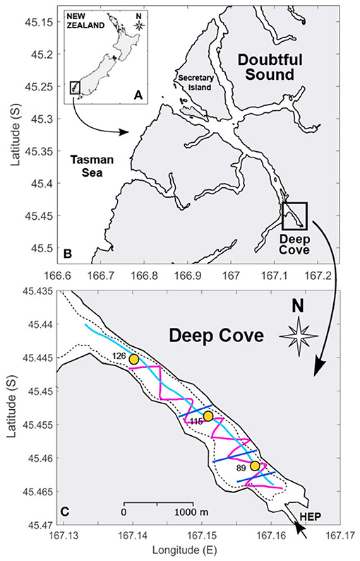
Figure 1. Location map of (A) New Zealand with the south-west Fiordland region highlighted, (B) Doubtful Sound and (C) Deep Cove showing the longitudinal (light blue), lateral (dark blue) and ‘zig-zag’ (pink) vessel transects. The placement of the September 2015 moorings are the circles. The arrow indicates the tailrace inflow from the Manapouri hydroelectric power station (HEP) and the thin dashed line is the 50 m depth contour. The lateral transects are 0.2 km, 0.5 km and 1.5 km downstream of the tailrace discharge point, respectively.

A freshwater tailrace carries discharge from the Manapouri hydroelectric power station into the head of Deep Cove (Figure 1C). The tailrace is the third largest river flow in New Zealand with an average inflow of Q = 420 m³ s⁻¹. Peak surface plume speeds are over 2 ms⁻¹ (McPherson et al., 2019) and comparable to the maximum outflow velocity of the Columbia River (Nash et al., 2009). The continuous tailrace inflow into the fjord represents an excess of twice the natural run-off, driven by an annual rainfall >7 m (Bowman et al., 1999), and results in highly stratified conditions. The freshwater input can produce similar vertical density gradients to those observed in major rivers such as the Columbia and Mzymta Rivers (Kilcher et al., 2012; Osadchiev, 2018). The depth of the freshwater surface layer is typically between 2 and 3 m thick (Gibbs, 2001).

3. Methods and analysis

The present observations were made during a 2-week long field campaign in March 2016. Over this period, tailrace discharge rates into Deep Cove were high and relatively steady (Q ≈ 530 m³ s⁻²) and the tidal range varied from 0.5 to 1.2 m (Figure 2). A range of instrumentation and observational techniques were applied to obtain a spatial distribution of the density and velocity fields within Deep Cove. The coordinate system used here is based in a channel reference frame, where x is the along-channel coordinate increasing with distance from the discharge point (x = 0) toward the end of Deep Cove, and y is the across-channel coordinate. This reference frame maintains consistency between the calculation of lateral plume spreading rates using the different methods outlined below.

FIGURE 2

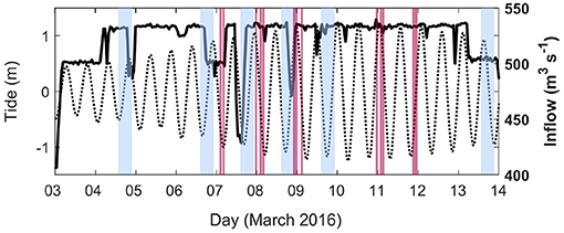
Figure 2. Hourly tailrace discharge rate (solid line) and tide (dashed) for the duration of the field experiment. Peak spring tide occurred on 11 March. The blue shaded boxes indicate the timing of the GPS drifter experiments and the red were the across-channel vessel transects.

3.1. Vessel-Based Survey

A sequence of vessel-based observations within Deep Cove were repeated over the course of the field campaign. Along-channel transects were aligned with the main river discharge, lateral transects cut through the plume perpendicular to its trajectory, and oblique (‘zig-zag’) transects captured both lateral and longitudinal plume evolution (Figure 1C). At least six consecutive lateral transects were repeated during each sampling period (Figure 2). Horizontal velocity estimates were obtained from a vessel-mounted ADCP (RDI Workhorse, 600 kHz) which sampled water velocities in 1 m vertical bins from 2.5 to 41.4 m. Near-surface velocities were obtained by applying a linear fit to the velocity data to extrapolate from 2.5 m to the surface. The extrapolated velocity profiles had compared well to in-situ near-surface velocity measurements from previous field campaigns (McPherson et al., 2019), and were in good agreement with surface plume velocities estimated by the Lagrangian GPS drifters. Currents were rotated according to the local bathymetry to determine along-channel (u) and across-channel (v) velocities. A weighted 10 m ‘bowchain’ was attached to the vessel which comprised temperature (RBRsolo) and CTD loggers (RBRconcerto) sampling at 2 and 5 Hz, respectively. High-resolution profiles of practical salinity and temperature were obtained from continuously profiling 'tow-yoed' CTD loggers (RBRconcerto). These data enabled estimation of the buoyancy frequency from the measured density profiles,

$\begin{array}{ll}N=\sqrt{-\frac{g}{\rho }\frac{\partial \rho }{\partial z}}& (2)\end{array}$

where ρ is the potential density.

The lateral transects of temperature from the bowchain were used to quantify vertical (K_z) and lateral (K_y) diffusion by estimating the change in thickness and width of the plume over distance, respectively. While salinity is generally used to identify and track freshwater plumes in coastal systems (Hetland, 2005), the persistent low-salinity surface layer observed throughout Deep Cove and the wider fjord region, resulting from the tailrace inflow and high rainfall (Gibbs, 2001), makes the distinction between the buoyant plume and freshwater surface layer less pronounced in the salinity field than in temperature (Figures 3C–E). Thus, temperature was used to define the plume boundaries in this study (Figures 3A,B). The diffusion components were therefore estimated by,

$\begin{array}{ll}{K}_y=\frac{\Delta y_{\text{p}}^2}{t_t}\text{ and }{K}_z=\frac{\Delta z_{\text{p}}^2}{t_t},& (3)\end{array}$

where t_t is the time taken for the plume to flow between each transect, y_p is the width of the plume at its base and z_p is the plume depth. The base of the plume is defined as the depth of maximum stratification. The depth of the plume is then defined as the distance from the base of the plume to the maximum height of the bounding isotherm.

FIGURE 3

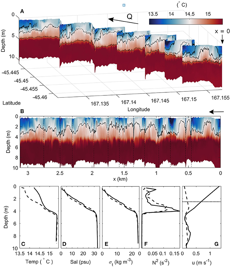
Figure 3. (A) Vertical and spatial distribution of temperature within Deep Cove, and (B) the expanded temperature timeseries of (A) with respect to distance from the discharge point. The horizonal lines in (B) separate each transect. Mean profiles of (C) temperature, (D) salinity, (E) density (σ_t), (F) buoyancy frequency-squared (N²), and (G) along-channel velocity (u) from inside (solid) and outside (dashed) the plume. The path of the transect relative to the fjord in (A) can be seen in Figure 1C. The 14, 14.5 and 15° C isotherms are shown in (A), and the 14.5° C isotherm in (B). The dotted line in (G) shows the depth above which the velocity was interpolated. The arrows in (A) and (B) indicate the direction of tailrace inflow (Q), from right to left.

3.2. GPS Drifters

Lagrangian measurements of near-surface currents were made during six GPS drifter experiments. The plume discharge rate and wind speeds for each experiment are detailed in Table 1, and wind direction was consistently up-fjord due to the surrounding steep topography. The headwaters of the fjord absorb the momentum of tidal oscillations (O'Callaghan and Stevens, 2015) and tides do not influence near-field mixing here (McPherson et al., 2019), thus the tidal impact on drifter trajectories is not considered.

TABLE 1

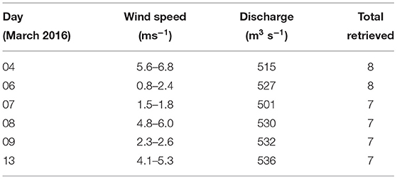
Table 1. Summary of drifter deployments and conditions.

The drifters each had a cylindrical drogue of height 0.5 m and diameter 0.2 m, and were ballasted to measure the upper 0.5 m of the water column by a small spherical float. Wind slippage was minimal as the float had little exposure to wind above the surface water level. Each drifter was equipped with a GPS receiver (Columbia V-900 GPS data logger) which recorded every 1 s. The GPS devices have a position accuracy up to 1.5 m, depending on satellite coverage. The drifters were released approximately 10 m apart across the width of the tailrace discharge point and were recovered after ~ 1 h. A total of 8 drifters were deployed in the first two experiments then, due to the loss of a GPS receiver, 7 drifters were deployed and retrieved in the subsequent four experiments.

The drifters were used to quantify the plume lateral spreading rate by estimating the change in plume width with distance from the discharge point, following a similar approach applied by Chen et al. (2009). The normalized plume width is given by W/W₀, where W is the plume width at a given location and W₀ is the width of the plume at a reference location. For drifter data, W is evaluated as the standard deviation of the distances between all drifters in the cross-plume direction at the given location. The plume width is then normalized by W₀. For each GPS drifter deployment, W₀ is taken as the first estimate of plume width (W) closest to the tailrace discharge point. This choice of W₀ enables W/W₀ for each drifter deployment to be compared, despite the variability in the deployment locations of the drifters in each experiment. For the lateral transects, W₀ = 100 m, which is the measured distance of the width of the tailrace discharge point (McPherson et al., 2020). Here, W is calculated along each drifter track at intervals of 10 m from the reference point. The uncertainty limits are the minimum and maximum standard deviations of all the subsets of the deployed drifters at each 10 m interval. The drifter method of estimating plume spreading is independent of drifter speed as plume width is evaluated as the distance between drifter tracks at a specified point from the reference point, and not at a given time.

Lateral dispersion is then quantified from the continuous convergence and divergence of drifters from the center of the plume. The standard deviation of the distance between the drifters and the plume centerline (σ_r), defined as the average drifter track, was used to calculate the diffusion coefficient,

$\begin{array}{ll}{K}_h(l)=\frac{d{{\sigma }_r}^2(t_d)}{2dt}& (4)\end{array}$

where t_d is the diffusion time (i.e., the time elapsed since the individual drifter deployment) and l = 3σ_r is the scale of diffusion (Okubo, 1971). Horizontal plume spreading is generally anisotropic thus ${\sigma }_r=\sqrt{({\sigma }_x^2+{\sigma }_y^2)}$, where σ_x, σ_y denote the standard deviations in the along and across-channel directions, respectively (Stocker and Imberger, 2003).

3.3. Moored Timeseries Data

Contributions to results in section 5.3.1 were from three near-surface moorings deployed in September 2015 (Figure 1C). Further details about this field campaign can be found in McPherson et al. (2019). Velocity measurements were obtained from an upwards-facing Acoustic Doppler Current Profiler at 10 m (ADCP; RDI Workhorse, 600 kHz), set to record an ensemble every 3 min in 2 m vertical bins. Spectral analysis was conducted on the velocity observations (Emery and Thomson, 2001) in which the time series was split into half-overlapping intervals equivalent to the inertial frequency, and the spectrum was computed using Welch's periodogram method.

3.4. Control Volume Methods

Plume lateral spreading rates can also be quantified using the control volume method, where measured quantities are connected to plume dynamics over a defined finite region of the flow field, termed a control volume. Freshwater conservation is applied to estimate plume width (b) in the control volume region (MacDonald and Geyer, 2004; Chen et al., 2009). Details of the control volume over the near-field plume region in Deep Cove can be found in McPherson et al. (2020). Horizontal scale-dependent dispersion is then determined from the growth of b with distance from the tailrace discharge point,

$\begin{array}{ll}b(x)={((2-n)\beta b_0^{1-n}x+b_0^{2-n})}^{1/(2-n)}& (5)\end{array}$

where β = 12α/(Ub₀) represents the magnitude of dispersion using the mean along-channel velocity U, and b₀ is the initial plume width (Fong and Stacey, 2003). A non-linear least squares fit of the control volume estimates of b to Equation (5) is taken and both β and n are treated as adjustable parameters. By optimising for n and α using this fit, these parameters can be compared to the empirical estimates from Equation (4). The method has been used to estimate horizontal dispersion in both near-coastal systems and the open ocean (Stacey et al., 2000; Fong and Stacey, 2003; Jones et al., 2008; Moniz et al., 2014).

4. Results

4.1. Near-Field Water Column Structure

Observations from the bowchain and tow-yoed CTD showed a highly-stratified upper water column with a 2 m thick freshwater (σ_t ≈ 1 kg m⁻³) surface layer overlaying a sharp density interface, and a dense, oceanic ambient (σ_t = 24 kg m⁻³) below 5 m (Figures 3B–E). The zig-zag temperature transects illustrate the evolving structure and path of the buoyant plume within the surface layer (Figure 3A). The 3 m thick plume was observed in the surface layer as a core of water approximately 1° C warmer than the 13.6°C ambient surface layer (Figures 3A–C). The plume boundary can thus be defined by an isotherm of 14.5°C. Maximum plume temperatures were found at the base of the surface layer, toward the core of the plume (~ 14.9°C) where warmer water was entrained from the ambient below (15.5°C) (Figure 3C). The plume was confined to the surface layer by strong salinity-induced stratification (N² = 10⁻¹ s⁻²) in the pycnocline (Figure 3F). Generally weaker values were observed within the plume layer (N² = 10⁻² s⁻²) and reduced toward zero with depth below the interface to 10 m.

The velocity structure of the near-field region was characterised by a fast-flowing surface plume with speeds over 1.5 ms⁻¹, which overlay a relatively stationary ambient below 5 m (Figure 3G). The ambient surface layer currents were weak (< 0.1 ms⁻¹), thus the outer plume boundary can also be defined by speeds of 0.2 ms⁻¹. The near-surface velocity field shows the plume decelerates as it propagates downstream. Maximum surface velocities at the plume centerline decreased from 1.05 ms⁻¹ to 0.2 km downstream of the tailrace discharge point to 0.81 and 0.65 ms⁻¹ at 0.5 and 1.5 km downstream, respectively, (Figure 4A). Flow speeds tended toward zero with lateral distance from the plume centerline, into the surrounding surface ambient. The near-surface plume measurements compared well to the velocities derived from the GPS drifters, estimated as the time derivative of the coordinate position. The drifters initially moved at speeds of ~ 1.7 ms⁻¹ near the tailrace discharge point and decreased to approximately 0.6 ms⁻¹ toward the seaward end of Deep Cove (Figure 5). Maximum speeds of over 2 ms⁻¹ were recorded near the discharge point.

FIGURE 4

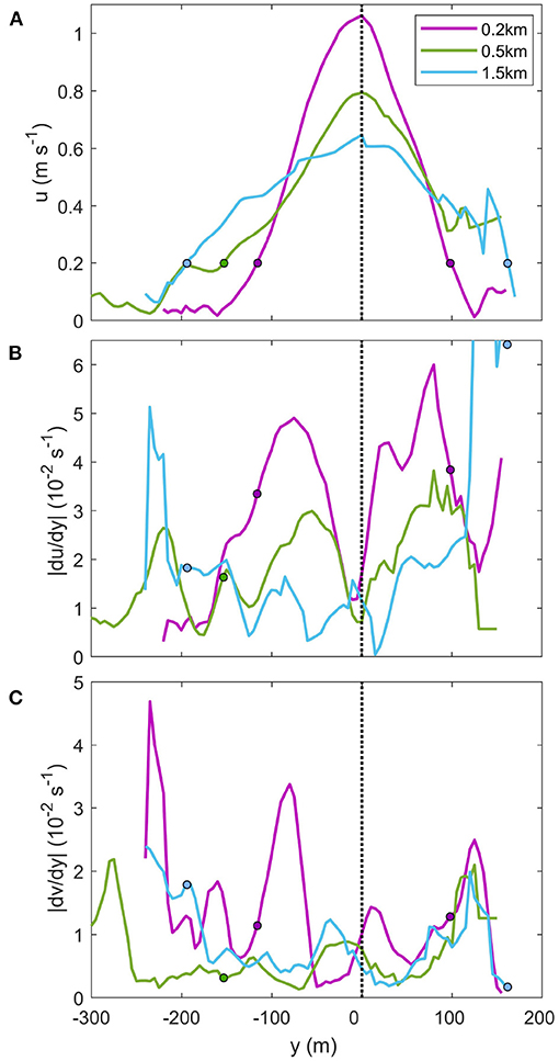
Figure 4. The evolving mean (A) across-stream velocity, and velocity shear of (B) along-channel and (C) across-channel velocities at downstream locations from the discharge point. Velocities are from 2.5 m below the surface. The across-channel distance (y) is relative to the centre of the plume, defined as the location of maximum u. The coloured circles represent the location of the plume edge, defined by 0.2 ms⁻¹. (A) The mean velocity transects were averaged over at least six consecutive lateral transects from the vessel-mounted ADCP on 09 March 2016.

FIGURE 5

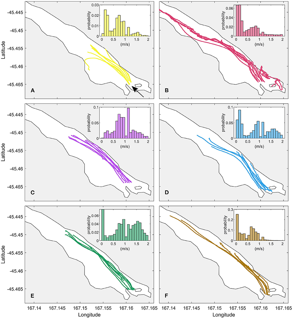
Figure 5. The trajectories of the multiple GPS drifters released near the entrance of the tailrace discharge point, where (A–F) are the six deployments, corresponding to the days outlined in Table 1, respectively. On the upper right corner of each plot is a histogram of flow velocities of all the drifters in each experiment (ms⁻¹). The histograms are normalised by the maximum of the distribution. The arrow in (A) indicates the tailrace discharge point and the direction of flow.

4.2. Techniques for Evaluating Lateral Plume Spreading

4.2.1. GPS Drifters

Estimates of plume width derived from the 6 GPS drifter deployments indicate an evolving plume structure as the plume propagates downstream (Figure 6). The drifter tracks show consistent behaviour over sections of the trajectories, with the plume width thinning and thickening over the same intervals. A general reduction in plume width from W/W₀ = 1 between the tailrace discharge point to 1 km downstream is observed in all transects, reaching a minimum of W/W₀ = 0.2, before the plume begins to spread laterally and W/W₀ increases toward 1 at 1.5 km. The three deployments that propagated further downstream show an overall decrease in W/W₀ toward 2.5 km. However, little to no lateral plume spreading occurred over the length of Deep Cove. The estimates of W/W₀ at the end of each transect were generally smaller than 1, with fluctuations of W/W₀ between 0.7and0.9 over the length of each deployment. This reflects the observed drifter trajectories where the majority of drifters remained within 10 m of each other over the duration of each experiment (Figure 5). The maximum W/W₀ = 3.4 occurred during the 04 March experiment when two drifters were detrained from the mean flow and diverged from the body of the drifter pack at approximately 1 km downstream from the inflow (Figure 5A).

FIGURE 6

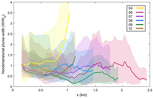
Figure 6. The non-dimensional plume width (W/W₀) for each GPS drifter experiment with respect to along-channel distance from the discharge point (x). The shaded regions indicate the uncertainty for each deployment. The drifter trajectories were averaged over 10 m.

4.2.2. Lateral Vessel Transects

The lateral spreading and evolving structure of the surface plume can be clearly identified in mean transects of temperature and velocity at increasingly downstream locations. Near the tailrace discharge point, the buoyant plume was a distinct symmetrical core of warmer water (> 14.5° C) within the 3 m thick ambient surface layer (Figure 7a). The surface layer overlays a sharp thermocline and well-mixed 15.5° C ambient water below 4 m. The plume width at 0.2 km from the discharge point was 268 m, compared to a fjord width of approximately 800 m. At 0.5 km downstream, the width of the near-symmetric core had increased to 312 m (Figure 7b) while, farther downstream at 1.5 km, the plume had spread almost uniformly across the vessel transect and had a width of 371 m (Figure 7c). The thermocline had become more diffuse with distance from the inflow and thickened down to 4.5 m.

FIGURE 7

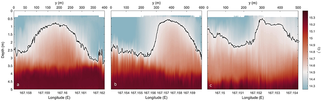
Figure 7. Mean vertical distribution of temperature of across-channel transects in the near-field plume region taken (a) 0.2 km, (b) 0.5 km and (c) 1.5 km downstream of tailrace discharge point. The plume boundary was defined by the isotherm 14.5°C (black lines), and the plume edge is indicated by the white circles on the isotherm. These edges were determined from the gradient of the depth of the isotherm. Temperature was recorded by the bowchain and averaged over at least six consecutive lateral transects.

The evolution of the near-surface velocity field also shows the lateral spreading of the plume. At the tailrace discharge point, the plume has a near-Gaussian appearance which flattens and spreads laterally as it propagates downstream (Figure 4A). The distance between the outer plume boundaries, here defined by 0.2 ms⁻¹, increased laterally from 225 to 355 m over the 1.3 km distance. Along and across-channel velocity shear at the base of the plume were derived using the vessel-mounted ADCP. Strong velocity shear occurs at either side of the plume centerline at each downstream transect, with peaks corresponding the location of the plume edges (0.2 ms⁻¹, Figure 4A), before tending toward zero both toward the plume centerline and into the surrounding ambient. Maximum values of |du/dy| ≈ |dv/dy| ≈ 10⁻² s⁻¹ peaked within 0.2 km of the tailrace discharge point, where plume speeds were greatest (u > 1 ms⁻¹) (Figure 4). The peaks of velocity shear decreased with distance from the discharge point as the plume decelerated and moved laterally away from the centreline as the plume spread. Farther downstream at 1.5 km, the maximum |du/dy| and |dv/dy| decreased by half and peaked toward the edges of the transect where the plume boundaries were approached (Figures 4B,C).

4.3. Techniques for Evaluating Dispersion

4.3.1. GPS Drifters

A diffusion diagram provides a means of predicting the rate of lateral spreading and the scale-dependence of the dispersion rates. Dispersion rates for the plume derived from the GPS drifters (using Equation 4) are shown as a function of their scale. As expected, the lateral component of dispersion (K_y) was much larger than the longitudinal dispersion (K_x) component, and both K_x and K_y increased with the scale of mixing (Figure 8). Estimates of K_x = 0.3 − 1.0 m² s⁻¹ were observed at diffusion scales of 0 < l < 120 m, while K_y was at least one order of magnitude greater for larger scales, ranging from K_y = 1.4 − 14.1 m² s⁻¹ between 10² < l < 10³ m. Expressing the estimates in the form of $K_h=\alpha l^n$ (Equation 1), the line of best fit yielded α = 0.0017 m^2/3 s⁻¹ and n = 1.38 ± 0.23. The errorbars show 95% confidence intervals of the slope over 1,000 bootstrap samples. Most of the latitudinal and longitudinal diffusion estimates fall within the 95% confidence intervals on either side of the predicted values.

FIGURE 8

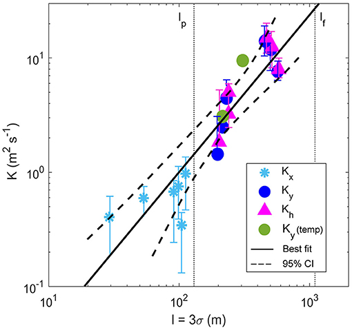
Figure 8. Okubo-style diffusion diagram of mean lateral (K_y, circles), longitudinal (K_x, stars) and total diffusion (K_h, triangles) against the scale of diffusion (l). All diffusion component estimates were derived from the 6 GPS drifter trajectories (Figure 5) and K_y from two sets of mean lateral temperature transects at the three downstream locations (green) (Figure 1C). Error bars denote a 95% bootstrap confidence interval of the slope (dashed lines). The two vertical lines (dotted) represent the average width of the plume (l_p) and the fjord (l_f).

4.3.2. Lateral Vessel Transects

Estimates of plume dispersion rates from the lateral vessel transects of temperature (Figure 7) can also be obtained. Using the 14.5° C isotherm as the plume boundary and applying Equation (3), the results provided an alternate estimate of K_y = 29.8 m² s⁻¹ and a vertical diffusion component of $K_z=1.4\times 10^{-4}$ m² s⁻¹ for the distance between the 0.2 and 1.5 km transects. This K_z is comparable to the vertical diffusivity measured in other river plumes (Hetland, 2005; Horner-Devine et al., 2009) which suggests that Equation (3) provides an accurate first-order estimate of bulk diffusion. The K_y estimates derived from both Figure 7 and other repeated lateral transects of temperature agree well with the drifter-derived horizontal diffusion results (Figure 8).

5. Discussion

5.1. Comparison of Spreading Rates Between Techniques

The rate of plume lateral spreading was quantified using two different observational methods; Lagrangian GPS drifters which measured near-surface plume velocities directly (Figure 6) and lateral transects of temperature and velocity fields (Figures 4, 7). These directly observed results can then be compared to estimates of plume width determined by a control volume method. This control volume technique used hydrographic observations from along and across-fjord transects, and is detailed in McPherson et al. (2020).

Estimates of plume width derived from the across-channel hydrographic transects generally compared well to the estimates derived from the control volume method (Figure 9). The control volume results show that W/W₀ increased from 1 close to the tailrace discharge point to W/W₀ = 1.8 over 3 km downstream, indicating that the plume spread laterally in the near-field region as it propagated seaward. The estimates of W/W₀ derived from the repeated lateral transects of temperature and velocity, using 14.5 ° C and 0.2 ms⁻¹ as the definitions of the plume boundary, respectively, correspond well at the three downstream locations. They all show a consistent increase in W/W₀ over the along-channel distance and are in good agreement with the control volume plume width estimates. The estimates of W/W₀ derived from the average GPS drifter trajectory (Figure 6) are generally smaller than the other observed values, suggesting an underestimation of plume width using this method.

FIGURE 9

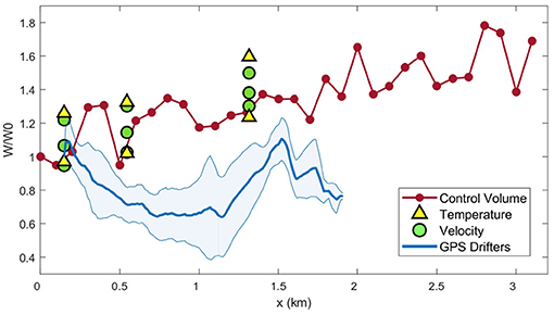
Figure 9. The evolution in non-dimensional plume width (W/W₀) with distance from the discharge point estimated by three observational methods: lateral transects of temperature (triangles) and velocity (circles), a control volume method (red) (McPherson et al., 2020) and the average W/W₀ calculated from the six GPS drifter deployments (Figure 6) (blue). The estimate of W for each method was normalized by W₀, where W₀ = 100 m for the transects and control volume, and W₀ = W(1) for the drifter deployments. The average plume width from the drifters was estimated with a minimum of three measurements for a standard deviation (shaded blue area).

While a general increase in W/W₀ over the length of Deep Cove was observed in both the control volume and transect data, the variability in the measurements highlights an evolving along-channel lateral spreading rate (db/dx). Over the total 3 km near-field region, db/dx = 0.045 from the control volume estimates. However, this rate increases and decreases over different sections of Deep Cove. All methods show an agreement in the evolving pattern of db/dx in the initial 1.5 km, with weaker horizontal spreading rates in the first 0.5 km and an increase toward 1.5 km. Further downstream, there is a slowing of plume spreading toward the end of Deep Cove. The highest lateral spreading rates are generally derived from between the lateral transects of temperature and velocity, with db/dx ≈ 0.05 between 0.2 and 0.5 km increasing to between 0.04 and 0.09 between 0.5 and 1.5 km. Estimates of db/dx from the control volume method are at the lower range over the same intervals, peaking at 0.05 at 1.5 km. While the corresponding horizontal spreading rate from the GPS drifters also shows this evolution of db/dx, with an initial weaker db/dx and an increased rate between 0.5 and 1.5 km, the estimates of db/dx remain one order of magnitude smaller than the control volume estimates over the length of the track. The good agreement between the estimates of plume width and db/dx from the control volume and lateral vessel transects (Figure 9) indicates that either the drifters underestimated the plume width, or in fact quantified a different process that was locked to the near-surface.

This change in db/dx in space is not surprising as the spreading rate is determined by the initial momentum from the variable plume inflow (Figure 2), the density difference between the freshwater surface layer and ambient water below, and the degree of vertical mixing at the interface (Chen et al., 2009). Thus the effect of the enhanced shear-driven mixing observed at the base of the plume (McPherson et al., 2019) which weakens the density gradient at the interface as the plume propagates downstream (Figure 7) would in turn reduce the lateral spreading rate.

The discrepancy between the results can be examined by considering what the GPS drifters actually measured in this field setting. While estimates of lateral spreading from drifters in other river plume systems have generally compared well to results from numerical and other observational techniques (Hetland and MacDonald, 2008; Chen et al., 2009; McCabe et al., 2009), drifters are also susceptible to meteorological and other oceanographic factors. A drifter consisting solely of a surface float with no drogue provides velocities and a trajectory that are a combination of surface advection, Stokes drift (an extra wave-induced force at the water surface) and direct wind forcing (Lumpkin et al., 2017). However, the impact of these external forcings on the GPS drifters used in the experiments conducted in Deep Cove were minimized by their design. The effects of wind on the trajectories of the drifters in Deep Cove was reduced by having very little of the drifter visible above the water, by conducting the GPS drifter experiments when wind speeds were low (Table 1), and by including a ballast centered at 0.5 m beneath the surface. The ballast also ensured the drifter was largely unaffected by the motion due to drift beneath the surface-wave-driven Stokes layer.

In Deep Cove, the drifters tended to remain clustered together within the body of the plume with no evidence of horizontal spreading (Figure 5). Over the initial 1 km, all drifter trajectories tended to show a decrease in plume width, before increasing further again downstream (Figure 6). The high flow speeds measured by the drifters (Figure 5) indicate the drifters remained within the main flow. The clustering of the drifters near the plume centerline is likely caused by a convergence of surface flow that concentrated the drifters in regions of high velocity within the center of the plume (Hetland and MacDonald, 2008).

The density and pressure gradients in the surface layer suggest this convergence of surface water occurred in the initial 1 km. Density and pressure in the surface layer are greatest within the center of the plume (Figure 3E) due to the enhanced entrainment of high density ambient water into the low density surface plume, driven by strong vertical mixing (McPherson et al., 2019). This vertical mixing creates a horizontal density gradient at the base of the plume. The corresponding horizontal baroclinic pressure gradient component is therefore greatest at 3 m below the surface, and peaked on either side of the plume centreline at both 0.25 and 1.5 km downstream of the inflow (Figure 10). The baroclinic pressure gradients tends toward zero at the surface. The barotropic pressure gradient also displays corresponding peaks at eiher side of the plume centerline, though the peaks of either pressure component are of an opposite sign.

FIGURE 10

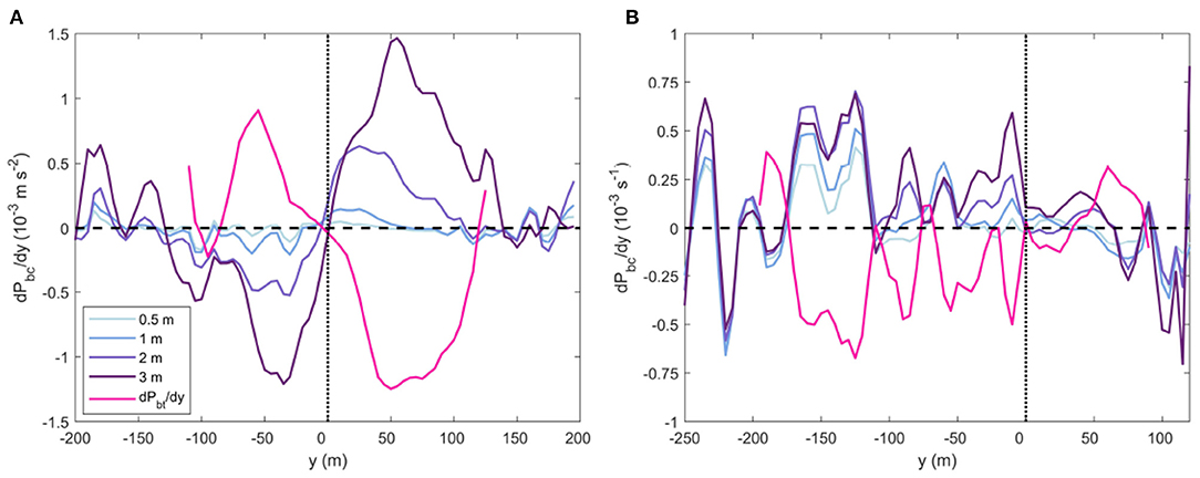
Figure 10. Horizontal baroclinic pressure gradient from within the plume layer at 0.5, 1, 2, and 3 m below the water surface, and barotropic pressure gradient (pink) at (A) 0.25 km and (B) at 1.5 km downstream of the tailrace discharge point (Figure 1C). The vertical dashed lines illustrates the centre of the plume.

By combining the across-channel baroclinic and barotropic pressure gradients, the total across-channel pressure gradient determines the direction and magnitude of the near-surface flow (Figure 11). At the surface, the total pressure gradient is dominated by the barotropic component, as the baroclinic pressure gradient is weakest at 0.5 m (Figure 11A). The positive total pressure gradient to the left of the plume centerline and the negative to the right indicates a strong flow converging toward the center of the plume. With depth, the baroclinic component increases and begins to influence the total pressure gradient, thus the direction of near-surface flow. A lateral diverging flow from the centre of the plume is already apparent at 2 m, while there is still exists a stronger converging flow outside 50 m (Figure 11C). At 3 m, the baroclinic component dominates the total pressure gradient (Figure 11D). This results in a strong lateral flow of plume water away from the centerline, driving the lateral spreading of the plume. The lateral velocity gradient (dv/dy) also illustrates diverging velocities at 2.5 m below the surface, peaking at the edges of the plume (Figure 4C).

FIGURE 11

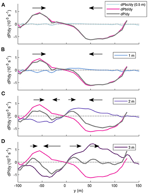
Figure 11. The balance of pressure gradient components within the surface layer at 0.2 km from the tailrace discharge point. The barotropic (pink) and baroclinic components sum to equal the total pressure gradient (grey). The baroclinic component is calculated at (A) 0.5 m, (B) 1 m, (C) 2 m, and (D) 3 m below the surface. The black arrows indicate the direction of the flow across the mean transect as a result of the total pressure gradient. The size of the tail of the arrow scales with the strength of the flow.

This balance of flow convergence toward the plume centerline at the near-surface and divergence from the centerline at the plume base can also be demonstrated in the Gaussian shape of the near-field plume in the lateral transects of temperature (Figure 7). The wider base illustrates the lateral spreading of the plume driven by the baroclinic pressure gradient, while the narrowing toward the water surface indicates the near-surface convergence.

Further downstream at 1.5 km, the role of the pressure gradient components are reversed (Figure 10B). The barotropic component drives a near-surface divergence of flow while the corresponding baroclinic pressure gradient shows a convergence of flow, the strength of which increases with depth. The barotropic pressure gradient tends to dominate throughout the surface layer which drives a total lateral spreading of the plume. This near-surface divergence of flow from the plume centerline is also reflected in the GPS drifter trajectories which show an increase of plume width from 1 to 1.5 km. The rate of plume spreading over this distance derived from the GPS drifters compared relatively well to db/dx from the control volume estimates (Figure 9). Toward the end of Deep Cove, the drifters measured a decrease in plume width (Figure 9) which suggests another reversal of the lateral pressure components and a convergence of near-surface flow.

These horizontal density, pressure and velocity gradients (Figures 3B, 4, 10, 11), and the structure of the plume (Figure 7), suggests that the GPS drifters, drogued to the upper 0.5 km, were concentrated within the plume core over the intial 1 km by near-surface convergence, driven by the barotropic pressure gradient. The clustering of drifters about the plume centerline and within the main flow (Figure 4) meant that both the plume width and lateral spreading rate were not accurately measured, but also that the drifters were then dominated by the strong along-channel advection, which was a dominant component of the plume dynamics along the whole 3 km near-field region (McPherson et al., 2020). This resulted in an underestimation of the overall lateral spreading rate by the drifters in comparison to the other observational methods (Figure 9). Further downstream, the barotropic pressure gradient acted to diverge the near-surface flow away from the centerline which produced a comparable lateral spreading rate to the other observational methods employed, before converging again toward the end of Deep Cove.

5.2. Comparison With Other River Plume Systems

While the drifters converged toward the plume centerline at the near-surface and tended to underestimate the plume width, the results from the hydrographic transects and control volume also suggest a slower lateral spreading rate than typically found in near-field settings. The coastal river plumes conventionally studied generally show radial expansion and splaying streamlines (Hetland and MacDonald, 2008; McCabe et al., 2009; Kakoulaki et al., 2020), and adhere to a horizontal spreading rate for a two-layer gravity current of $\sqrt{(g^{\prime }H)/2}$ (Farmer et al., 2002). In the near-field region of Deep Cove, where g′ is calculated using an across-channel Δσ_t from Figure 3E, this equates to a bulk horizontal spreading rate of ~ 0.19 ms⁻¹. With a mean along-channel plume velocity of 0.8 ms⁻¹, the plume would theoretically spread by ~ 450 m over the 3 km near-field region (db/dx = 0.15). However, the observational results did not agree with these estimates. The plume width increased from 105 to 240 m over the length of Deep Cove, with a total spreading rate that was slower than theoretical rate by one order of magnitude (db/dx = 0.045 m⁻¹, Figure 9).

The difference between these lateral spreading rates could be attributed in part to the intense vertical mixing at the base of the plume in Deep Cove. Enhanced turbulent mixing has been shown to drive interfacial stress which is a dominant force acting to decelerate the near-field plume (Chen et al., 2009; McCabe et al., 2009; McPherson et al., 2020). The deceleration is controlled by entraining low-momentum ambient water into the surface layer, simultaneously mixing high-density ambient water into the freshwater surface layer, thus reducing the density gradient and slowing lateral spreading (Hetland, 2010). In comparison to typical estimates of ϵ in coastal environments, the measurements observed in the near-field region of Deep Cove are orders of magnitude greater. The highly stratified interface (N² = 10⁻¹ s⁻², Figure 3F) supports the intense shear generated by the high flow speeds (u > 1.5 ms⁻¹, Figure 3G), resulting in surface-intensified turbulence (ϵ > 10⁻³ W kg⁻¹) (McPherson et al., 2019). This corresponds to enhanced surface-intensified turbulence stress, over one order of magnitude greater than the peak stress in the Columbia River (Kilcher et al., 2012).

Comparing the balance of terms in a near-field momentum budget between Deep Cove and the Columbia River shows that the enhanced vertical mixing in Deep Cove is likely linked to the reduced corresponding lateral spreading rate. In the Columbia River, where internal stress was weaker, the role of lateral spreading in balancing the total momentum budget was much greater than in Deep Cove. The spreading term balanced the acceleration terms in the surface layer, and the internal stress divergence drove the deceleration. This translates to a greater lateral spreading rate in the Columbia River, db/dx = 0.16 (Kilcher et al., 2012), which was one order of magnitude larger than in Deep Cove. In Deep Cove however, where turbulence stress was high, the spreading term was negligible and the internal stress similarly controlled the plume deceleration. The balance of dynamics in each near-field setting suggests that the increase in internal stress reduces the spreading rate. When the internal stress increases relative to the other near-field processes, the enhanced turbulence at the interface drives a reduction in the density difference between the ambient and surface and therefore a reduced lateral spreading rate. Thus, the high ϵ in Deep Cove could be responsible for the slower horizontal spreading than typically observed for near-field plumes with weaker turbulent mixing.

While the enhanced turbulent mixing at the base of the plume in the near-field is likely to reduce the rate of lateral plume spreading, the surrounding topography and its impact on plume evolution is also relevant in this system. The trajectories of the GPS drifters highlight the proximity of the fjord sidewalls to the mean plume flow (Figure 5). While the role of the sidewalls on the lateral plume spreading rate cannot be quantified, they are able to explain the circulation pattern in the surface layer by driving the barotropic pressure gradient and convergence of near-surface flow. The plume spreads laterally, from high to low pressure, as it propagates downstream (Figure 10). However, the sidewalls act as a physical barrier which prevents the continued and uninhibited lateral spreading of the plume. As the strong vertical density gradients (Figures 3E,F) also prohibit the downwelling of the surface ambient water, the surface water is then pushed up against the fjord sidewalls and increases the water height there. This creates a barotropic pressure gradient across the width of Deep Cove which drives the water back toward the center of the fjord and the plume. However, as the baroclinic pressure gradient is zero at the surface but greater than the barotropic component at 3 m (Figure 11), the water converges at the surface but is forced to diverge laterally at the base of the plume.

However, a uniform convergence of near-surface flow along the fjord was not observed. The lateral pressure gradient components showed a transition from near-surface convergence in the initial 0.25 km to divergence further downstream at 1.5 km (Figure 10) which was reflected in the trajectories of the GPS drifters as they propagated downstream (Figure 6). This along-channel change in near-surface flow could also be attributed to the sidewalls driving a form of oscillatory motion, such as a seiche, which propagates throughout the fjord basin. The initial expansion of the plume as it enters the fjord, no longer confined by the tailrace channel, forces the surrounding ambient water toward the fjord sidewalls. The barotropic pressure gradient is formed as described above and drives the near-surface convergence. However, this returning flow toward the center of plume could also be an oscillation which continues to propagate downstream and move laterally, impacting the barotropic pressure gradient and thus the drivers of plume spreading, reflected in the trajectories of the GPS drifters. However, the current spatial and temporal resolution of the data is unable to fully resolve any basin-wide oscillatory motion and its impact on the plume. The change in the fjord topography also impacts the plume spreading. The fjord is wider between 0.25 and 1 km as a bay exists to the south of the inflow (Figure 1C), before narrowing further downstream. As described above, the sidewalls restrict lateral spreading of both the plume and the surface ambient, thus any narrowing or widening of the sidewalls relative to the location of the plume would also affect the lateral pressure gradients and spreading.

There have been no observational field studies of the spreading dynamics of topographically-constrained plumes; river plumes typically studied generally exhibit a discharge perpendicular to the coast with no lateral boundaries (Yankovsky, 2000; Hetland and MacDonald, 2008; Chen et al., 2009; Kakoulaki et al., 2020). However, a change in drifter patterns was observed when GPS and modelled drifters, deployed near the mouth of a weakly-stratified tidal inlet, left the constrained tidal channel and reached the mouth of the inlet (Spydell et al., 2015). Within the channel, the drifters were generally retained in the main flow while, upon exiting the inlet, the lateral spreading rates increased. While a decrease in flow velocities with downstream distance was observed, which could balance the increase in horizontal spreading, the impact of the channel walls on the drifter trajectories and spreading rate were not considered. It is not unlikely that the same barotropic pressure gradient, from the increased sea surface height at the sidewalls of the channel, produced a convergence of flow which contributed to the drifters clustering together in the main flow. Though the fjord sidewalls appear to influence the near-surface circulation in Deep Cove, the relative roles of the enhanced turbulence and topography on the reduced lateral spreading rate relative to other plume systems remains unclear.

5.3. Lateral Dispersion

While advection governs the evolution and transport of the along-channel flow (Kilcher et al., 2012; McPherson et al., 2020), diffusion processes determine the across-channel transport in the near-field. Thus the processes responsible for the observed lateral spreading of the plume (Figure 9) can be examined by quantifying horizontal dispersion. A number of theoretical models describe dispersion by defining different drivers. The plume growth is characterised by an exponent of n = 4/3 which is the value expected for three-dimensional turbulence (Fong and Stacey, 2003). Turbulence theory postulates that dispersion depends on the length scale of the motions and rate of turbulent dissipation (Batchelor, 1952), while shear-flow theory considers vertical diffusion in a horizontally sheared flow, driven by turbulence, as the governing process (Taylor, 1953; Fischer et al., 1979). Both theories are capable of producing a 4/3 power law, suggestive of scale-dependent growth (Stommel, 1949; Batchelor, 1950), and both are assessed here, to determine which is capable of representing the observed lateral spreading.

The scale-dependence of the observed lateral dispersion must be first examined to determine if the n = 4/3 power law is met, thus if these models are suitable. The slope of the best-fit of the lateral diffusion estimates, n, defines the scale-dependence of the dispersion. The diffusion diagram is first examined, which combines estimates of diffusion from the GPS drifters and hydrographic transects (Figure 8). Based on scale, the estimates of lateral diffusion observed here are comparable to other plume inflows (Yankovsky, 2000; Hunt et al., 2010). The line of best-fit applied to these estimates yielded n = 1.38 ± 0.23. This observed n is not inconsistent with, and indeed compares relatively well to, the theoretical n = 4/3 which suggests scale-dependent behaviour following the 4/3 law.

Furthermore, the plume width model (Equation 5), using estimates of b derived from the control volume, can also be used to quantify the plume's scale-dependent lateral dispersion. A non-linear least-squares fit of b is applied to Equation (5), setting b₀ = 128 m and U = 1.1 ms⁻¹, and optimising for n and β, gives a best-fit of n = 1.39 ± 0.35 and β = 0.024 ± 0.005 (Figure 12). Most of the plume width estimates fall within the 95% confidence intervals on either side of the predicted values given the optimised parameters. The close agreement of n between the diffusion diagram and plume width model results indicate that, within statistical certainty, n = 4/3, and independently supports the empirical dispersion coefficient from the diffusion diagram. Thus, both turbulence and shear-driven theoretical models can be examined in order to determine the drivers of lateral dispersion.

FIGURE 12

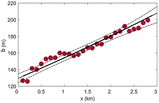
Figure 12. Plume width (b) as a function of distance from the tailrace discharge point. The best-fit line with scale-dependency n = 1.39 ± 0.35 (solid) was determined using the length-scale model of Equation (5). Dashed lines are the 95% confidence limits of the line of best fit.

5.3.1. Dispersion From Turbulence Theory

The initial dispersion in the near-field plume is governed by a 4/3 power law, which is the exponent expected for three-dimensional turbulence. Furthermore, the enhanced turbulent mixing observed in the near-field of this system and its dominant role in controlling the structure and behaviour of the plume (McPherson et al., 2019, 2020), including its likely impact on the reduction of lateral plume spreading, motivates the analysis of dispersion first using turbulence theory. The turbulence model can be examined based on its assumption that dispersion depends on the length scale of turbulence, i.e., the plume lateral length scale is related to the distance from the discharge point (Equation 5). Fixing n = 4/3, thus eliminating n as a fitting coefficient in Equation (5), gives β = 0.023 ± 0.002, where β is the magnitude of horizontal dispersion. This value of β is comparable to results from a near-bed plume in coastal waters where β = 0.02 (Stacey et al., 2000) and β = 0.036 (Fong and Stacey, 2003), suggesting the turbulence theory produces reasonable estimates of dispersion for a near-field buoyant plume.

However, the underlying assumption of the theory that the motions driving dispersion are found in the inertial subrange, thus turbulence governs lateral dispersion, must be considered. The length-scale model assumes that the plume is dispersed by three-dimensional turbulence structures, i.e., as the plume grows in scale, it is dispersed by progressively larger eddies (Fong and Stacey, 2003). To examine the scale of the dispersive motions in the surface layer, spectral analysis was conducted on velocity observations from the near-surface mooring deployed approximately 1 km downstream of the tailrace discharge point. The spectral fall-off rate varied with frequency (σ). A steep spectral slope of –3 was observed throughout the low-frequency range of the band (σ < f, where f is the Coriolis frequency) and transitioned to a slope of -5/3 for the higher frequency band (σ > 4f) (Figure 13). The –5/3 slope suggests a mean dominance of turbulence in the surface layer.

FIGURE 13

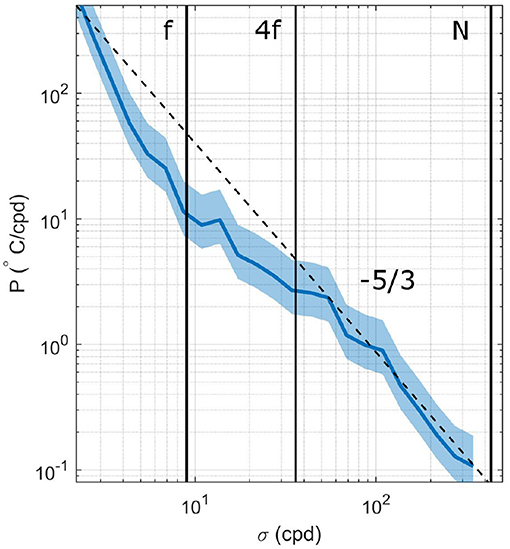
Figure 13. Power spectral density measurements of the along-channel near-surface flow (z = 2 m) approximately 1 km downstream from the tailrace discharge point. The vertical lines indicate the focus on the [f,N] range, and the −5/3 slope is shown as the dashed line. Variability lies within the 95% confidence interval (shaded region around the spectrum). The time series was split into half-overlapping intervals equivalent to the inertial frequency.

In the surface layer of a stratified river plume, the largest eddies scale with the depth of the surface layer due to the strong salinty-induced stratification (McPherson et al., 2019). The vertical velocity fluctuations are constrained to the thickness of the surface layer and, as the width of the plume far exceeds the vertical scales, forces the turbulence to be essentially two-dimensional (in the horizontal plane). The vertical plume scales which correspond to f = 10³ cpd (Tennekes and Lumley, 1972) fall outside of the inertial subrange thus the length-scale assumption is invalid. Therefore, while turbulence is in part responsible for the observed dispersion in the near-field plume region, hence n = 4/3 and a −5/3 energy spectrum, the lateral dispersion cannot be adequately described by turbulence theory.

5.3.2. Shear Flow Dispersion

An alternative to turbulence-driven dispersion is shear flow dispersion, which also yields a 4/3 power law dependence (Fischer et al., 1979). Shear dispersion arises from vertical mixing acting upon horizontally sheared flow (Taylor, 1953) and has been observed to be an important mechanism of dispersion in lakes and the ocean (LaCasce and Bower, 2000; Stocker and Imberger, 2003; Stevens et al., 2004; Moniz et al., 2014). The flow conditions in the near-field region support shear-flow dispersion, i.e., the strong velocity shear on either side of the plume centreline (|du/dy| = 10⁻² s⁻¹) highlights the presence of a sheared region between the plume interior and ambient surface layer (Figure 4B). These shear regions were most pronounced at 0.2 km from the tailrace discharge point and weakened with distance downstream as the plume decelerated. This deceleration was due to the entrainment of stationary ambient water into the fast-flowing surface layer by enhanced vertical mixing (ϵ > 10⁻³ W kg⁻¹) which exists throughout the near-field region (McPherson et al., 2020). Thus this combination of processes allows for the existence of shear-flow dispersion (Young et al., 1982).

Estimates of horizontal shear dispersion for a mean flow in the along-channel (x) direction can be derived (Fischer et al., 1979),

$\begin{array}{ll}{K}_x=1.5c_2{(\partial u/\partial y)}^2{\kappa }_y{t}_e^2& (6)\end{array}$

where c₂ = 0.037 (Saffman, 1963), t_e is the elapsed time, and κ_y is the horizontal diffusivity associated with the small-scale motions (Okubo and Ebbesmeyer, 1976). An equivalent expression applies for the across-channel (y) direction. The near-surface flow speeds were estimated from the lateral velocity transects, and estimates of κ_x = 0.3 and κ_y = 0.2 m² s⁻¹ were derived using the GPS drifters. The resultant horizontal along and across-channel shear dispersion coefficients, K_x = 0.2 and K_y = 15.8 m² s⁻¹, respectively, were the same order of magnitude as the empirical estimates of K_x and K_y from drifters and hydrographic transects (Figure 8). Furthermore, the magnitude of K_h from the horizontal shear dispersion coefficients was over 90% of the maximum dispersion coefficient from empirical estimates. This suggests that horizontal shear dispersion was the dominant mechanism responsible for the observed lateral dispersion in the surface layer of the near-field plume.

6. Summary

This study presents estimates of the lateral spreading rate of a near-field buoyant plume discharged into the head of a fjord. The plume system is characterised by flow speeds of over 2 ms⁻¹, and strong stratification (N² > 0.1 s⁻²), resulting in enhanced shear which supports the elevated turbulence dissipation rates (ϵ > 10⁻³ W kg⁻¹) at the base of the surface layer. The plume spreads horizontally at a rate of db/dx = 0.045 from the tailrace discharge point to 3 km downstream, which is one order of magnitude weaker than the theoretical spreading rate. This discrepancy is likely attributed to a combination of the enhanced internal stress and the presence of the fjord sidewalls. The vertical mixing at the interface drives a reduction in the density gradient between the dense ambient and freshwater surface layer and slows lateral spreading. The fjord sidewalls create a barotropic pressure gradient which drives a convergence of near-surface flow back toward the center of the fjord and the plume. The enhanced vertical mixing and reduced lateral spreading rates in Deep Cove highlight the interplay between these governing processes in a highly stratified and turbulent near-field plume system, and how their balance determines the ultimate structure and behaviour of the plume.

Results showed good agreement of estimates of plume widths between the cross-plume hydrographic data and estimates derived from a control volume method, while the GPS surface drifters underestimated the plume lateral spreading rate over the initial 2 km by a factor of ~ 10. This discrepancy was the result of a change in the dominance of pressure gradient components with depth. At the near-surface, a strong barotropic pressure gradient drove flow convergence toward the center of the plume and concentrated the drifters in regions of high velocity in the plume core. There, the drifters were dominated by along-channel advection and did not effectively measure lateral processes. Toward the base of the plume, a baroclinic pressure gradient dominated the barotropic component and drove lateral flow divergence at the interface. Further downstream, the barotropic pressure gradient component drove lateral spreading at both the near-surface and base of the plume. Both the control volume and lateral transects measured plume width at the plume base thus captured this lateral spreading.

Empirical diffusion estimates indicated that the lateral dispersion of this near-field plume increased with distance from the source, consistent with scale-dependent dispersion. A turbulence model and shear-flow dispersion model independently corroborated the 4/3 law of dispersion, which indicates that open ocean dispersion theory can be applicable in the near-shore coastal environment where stratification and vertical mixing are elevated. The strong stratification constrains the vertical dispersion of scalars while turbulence, which dominates the surface layer, acts on the strong horizontal shear between the plume interior and ambient surface layer to drive lateral dispersion. Horizontal shear dispersion that was responsible for over 90% of total diffusion within the surface layer. These results can be applied to other estuarine and coastal regimes as dispersion govern the fate of scalars, such as nutrients and contaminants, discharged into the coastal ocean. The presence of the steep fjord sidewalls means that these drivers of lateral spreading can also be applied to constrained systems, such as tidal inlets where tidal forcing produces strong currents in relatively narrow channels.

However, the work also highlights the sensitivity of observational methods to highly energetic systems and the complexity of the interactions between near-field physical processes such as plume mixing, shear and spreading. The combination of observational techniques appears to resolve and isolate lateral plume spreading, and quantify shear-driven dispersion. However, further numerical work is required to determine the relative role that turbulent mixing and lateral boundaries play to constrain the horizontal spreading. Improved understanding of these issues will also enable a better understanding of the behaviour and evolution of the near-field plume, and the ultimate fate and impact of the riverine waters.

Data Availability Statement

The original contributions presented in the study are included in the article/supplementary materials, further inquiries can be directed to the corresponding author/s.

Author Contributions

RM, CS, JO'C, and AL collcted the data. AL and JN contributed instrumentation and support to the field campaign, which was planned by RM and CS. RM treated and analysed the data, and wrote the manuscript. RM, CS, and JO'C discussed the results. CS, AL, and JN reviewed the previous drafts of the manuscript. All authors contributed to the article and approved the submitted version.

Funding

This research has been supported by the New Zealand Royal Society Marsden Fund (grant no. NIW-1301-2015) and the New Zealand Sustainable Seas National Science Challenge (project no. 4.2.2). The National Institute of Water and Atmospheric Research Strategic Science Investment Fund, and supported by the National Institute of Water and Atmospheric Research (NIWA).

Conflict of Interest

The authors declare that the research was conducted in the absence of any commercial or financial relationships that could be construed as a potential conflict of interest.

Acknowledgments

We would like to thank Brett Grant, Mike Brewer, Tyler Hughen, and June Marion, who helped with the 2016 field experiments, and Meridian Energy for providing the tail-race flow data. We thank the Reviewers for their extensive comments which where very helpful in improving the manscript. Bill Dickson and Sean Heseltine from the University of Otago skippered the vessels for the duration of the field campaign. Also thanks to Natalie Robinson for the use and field practice of the GPS drifters.

References

Batchelor, G. K. (1950). The application of the similarity theory of turbulence to atmospheric diffusion. Q. J. R. Meteorol. Soc. 76, 133–146. doi: 10.1002/qj.49707632804

CrossRef Full Text | Google Scholar

Batchelor, G. K. (1952). Diffusion in a field of homogeneous turbulence. Math. Proc. Cambridge Philos. Soc. 48, 345–362. doi: 10.1017/S0305004100027687

CrossRef Full Text | Google Scholar

Bowman, M., Dietrich, D., and Mladenov, P. (1999). Predictions of circulation and mixing in Doubtful Sound, arising from variations in runoff and discharge from the Manapouri power station, in Coastal Ocean Prediction, Vol. 56, Coastal and Estuarine Studies, ed Mooers, C. N. K., (Washington, DC: American Geophysical Union), 59–76.

Google Scholar

Chen, F., MacDonald, D. G., and Hetland, R. D. (2009). Lateral spreading of a near-field river plume: Observations and numerical simulations. J. Geophys. Res. 114:C07013. doi: 10.1029/2008JC004893

CrossRef Full Text | Google Scholar

Durand, N., Fiandrino, A., Fraunié, P, Ouillon, S., Forget, P., and Naudin, J. J. (2002). Suspended matter dispersion in the Ebro ROFI: an integrated approach. Contin. Shelf Res. 22, 267–284. doi: 10.1016/S0278-4343(01)00057-7

CrossRef Full Text | Google Scholar

Emery, W. J., and Thomson, R. E. (2001). Data Analysis Methods in Physical Oceanography. 2nd edn, Amsterdam: Elsevier.

Google Scholar

Farmer, D., Pawlowicz, R., and Jiang, R. (2002). Tilting separation flows: a mechanism for intense vertical mixing in the coastal ocean. Dyn. Atmosph. Oceans 36, 43–58. doi: 10.1016/S0377-0265(02)00024-6

CrossRef Full Text | Google Scholar

Fischer, H., List, J., Koh, C., Imberger, J., and Brooks, N. (1979). Mixing in Inland and Coastal Waters. New York, NY: Academic Press.

Google Scholar

Fong, D. A., and Stacey, M. T. (2003). Horizontal dispersion of a near-bed coastal plume. J. Fluid Mech. 489:S002211200300510X. doi: 10.1017/S002211200300510X

CrossRef Full Text | Google Scholar

Garvine, R. W. (1987). Estuary plumes and Ffonts in shelf waters: a layer model. J. Phys. Oceanogr. 17, 1877–1896. doi: 10.1175/1520-0485(1987)017<1877:EPAFIS>2.0.CO;2

CrossRef Full Text | Google Scholar

Gibbs, M. T. (2001). Aspects of the structure and variability of the low-salinity-layer in Doubtful Sound, a New Zealand fiord. N. Z. J. Mar. Freshwater Res. 35, 59–72. doi: 10.1080/00288330.2001.9516978

CrossRef Full Text | Google Scholar

Hetland, R. D. (2005). Relating river plume structure to vertical mixing. J. Phys. Oceanogr. 35, 1667–1688. doi: 10.1175/JPO2774.1

CrossRef Full Text | Google Scholar

Hetland, R. D. (2010). The effects of mixing and spreading on density in near-field river plumes. Dyn. Atmos. Oceans 49, 37–53. doi: 10.1016/j.dynatmoce.2008.11.003

CrossRef Full Text | Google Scholar

Hetland, R. D., and MacDonald, D. G. (2008). Spreading in the near-field Merrimack River plume. Ocean Model. 21, 12–21. doi: 10.1016/j.ocemod.2007.11.001

CrossRef Full Text | Google Scholar

Horner-Devine, A. R., Jay, D. A., Orton, P. M., and Spahn, E. Y. (2009). A conceptual model of the strongly tidal Columbia River plume. J. Mar. Syst. 78, 460–475. doi: 10.1016/j.jmarsys.2008.11.025

CrossRef Full Text | Google Scholar

Hunt, C. D., Mansfield, A. D., Mickelson, M. J., Albro, C. S., Geyer, W. R., and Roberts, P. J. (2010). Plume tracking and dilution of effluent from the Boston sewage outfall. Mar. Environ. Res. 70, 150–161. doi: 10.1016/j.marenvres.2010.04.005

PubMed Abstract | CrossRef Full Text | Google Scholar

Jones, N. L., Lowe, R. J., Pawlak, G., Fong, D. a., and Monismith, S. G. (2008). Plume dispersion on a fringing coral reef system. Limnol. Oceanogr. 53, 2273–2286. doi: 10.4319/lo.2008.53.5_part_2.2273

CrossRef Full Text | Google Scholar

Kakoulaki, G., MacDonald, D. G., and Cole, K. (2020). Calculating lateral plume spreading with surface Lagrangian drifters. Limnol. Oceanogr. Methods 18, 346–361. doi: 10.1002/lom3.10356

CrossRef Full Text | Google Scholar

Kilcher, L. F., Nash, J. D., and Moum, J. N. (2012). The role of turbulence stress divergence in decelerating a river plume. J. Geophys. Res. Oceans 117:C05032. doi: 10.1029/2011JC007398

CrossRef Full Text | Google Scholar

LaCasce, J. H., and Bower, A. (2000). Relative dispersion in the subsurface North Atlantic. J. Mar. Res. 58, 863–894. doi: 10.1357/002224000763485737

CrossRef Full Text | Google Scholar

Lumpkin, R., Özgökmen, T., and Centurioni, L. (2017). Advances in the application of surface drifters. Ann. Rev. Mar. Sci. 9, 59–81. doi: 10.1146/annurev-marine-010816-060641

CrossRef Full Text | Google Scholar

MacDonald, D. G., and Chen, F. (2012). Enhancement of turbulence through lateral spreading in a stratified-shear flow: development and assessment of a conceptual model. J. Geophys. Res. Oceans 117:C05025. doi: 10.1029/2011JC007484

CrossRef Full Text | Google Scholar

MacDonald, D. G., and Geyer, W. (2004). Turbulent energy production and entrainment at a highly stratified estuarine front. J. Geophys. Res. 109:C05004. doi: 10.1029/2003JC002094

CrossRef Full Text | Google Scholar

MacDonald, D. G., Goodman, L., and Hetland, R. D. (2007). Turbulent dissipation in a near-field river plume: a comparison of control volume and microstructure observations with a numerical model. J. Geophys. Res. 112:C07026. doi: 10.1029/2006JC004075

CrossRef Full Text | Google Scholar

McCabe, R. M., Hickey, B. M., and MacCready, P. (2008). Observational estimates of entrainment and vertical salt flux in the interior of a spreading river plume. J. Geophys. Res. 113:C08027. doi: 10.1029/2007JC004361

CrossRef Full Text | Google Scholar

McCabe, R. M., MacCready, P., and Hickey, B. M. (2009). Ebb-tide dynamics and spreading of a large river plume. J. Phys. Oceanogr. 39, 2839–2856. doi: 10.1175/2009JPO4061.1

CrossRef Full Text | Google Scholar

McPherson, R. A., Stevens, C. L., and O'Callaghan, J. M. (2019). Turbulent scales observed in a River Plume entering a Fjord. J. Geophys. Res. Oceans 124, 9190–9208. doi: 10.1029/2019JC015448

CrossRef Full Text | Google Scholar

McPherson, R. A., Stevens, C. L., O'Callaghan, J. M., Lucas, A. J., and Nash, J. D. (2020). The role of turbulence and internal waves in the structure and evolution of a near-field river plume. Ocean Sci. 16, 799–815. doi: 10.5194/os-16-799-2020

CrossRef Full Text | Google Scholar

Moniz, R. J., Fong, D. A., Woodson, C. B., Willis, S. K., Stacey, M. T., and Monismith, S. G. (2014). Scale-dependent dispersion within the stratified interior on the shelf of northern Monterey Bay. J. Phys. Oceanogr. 44, 1049–1064. doi: 10.1175/JPO-D-12-0229.1

CrossRef Full Text | Google Scholar

Nash, J. D., Kilcher, L. F., and Moum, J. N. (2009). Structure and composition of a strongly stratified, tidally pulsed river plume. J. Geophys. Res. 114:C00B12. doi: 10.1029/2008JC005036

CrossRef Full Text | Google Scholar

O'Callaghan, J. M., and Stevens, C. L. (2015). Transient river flow into a fjord and its control of plume energy partitioning. J. Geophys. Res. Oceans 120, 3444–3461. doi: 10.1002/2015JC010721

CrossRef Full Text | Google Scholar

Okubo, A. (1968). Some Remarks on the importance of the shear effect on horizontal diffusion. J. Oceanogr. Soc. Jpn 24, 60–69. doi: 10.5928/kaiyou1942.24.60

CrossRef Full Text | Google Scholar

Okubo, A. (1971). Oceanic diffusion diagrams. Deep Sea Res. Oceanogr. Abstracts 18, 789–802. doi: 10.1016/0011-7471(71)90046-5

CrossRef Full Text | Google Scholar

Okubo, A., and Ebbesmeyer, C. C. (1976). Determination of vorticity, divergence, and deformation rates from analysis of drogue observations. Deep Sea Res. Oceanogr. Abstracts 23, 349–352. doi: 10.1016/0011-7471(76)90875-5

CrossRef Full Text | Google Scholar

Osadchiev, A. A. (2018). Small mountainous rivers generate high-frequency internal waves in coastal ocean. Sci. Rep. 8, 16609. doi: 10.1038/s41598-018-35070-7

PubMed Abstract | CrossRef Full Text | Google Scholar

Richardson, L. F. (1926). Atmospheric diffusion shown on a distance-neighbour graph. Proc. R. Soc. A Math. Phys. Eng. Sci. 110, 709–737. doi: 10.1098/rspa.1926.0043

CrossRef Full Text | Google Scholar

Roberts, P. J. W. (1999). Modeling mamala bay outfall plumes. I: near field. J. Hydraulic Eng. 125, 564–573. doi: 10.1061/(ASCE)0733-9429(1999)125:6(564)

CrossRef Full Text | Google Scholar

Saffman, P. G. (1963). The effect of wind shear on horizontal spread from an instantaneous ground source. Q. J. R. Meteorol. Soc. 89, 293–295. doi: 10.1002/qj.49708938016

CrossRef Full Text | Google Scholar

Spydell, M., Feddersen, F., Guza, R. T., and Schmidt, W. E. (2007). Observing surf-zone dispersion with drifters. J. Phys. Oceanogr. 37, 2920–2939. doi: 10.1175/2007JPO3580.1

CrossRef Full Text | Google Scholar

Spydell, M. S., Feddersen, F., Olabarrieta, M., Chen, J., Guza, R. T., Raubenheimer, B., et al. (2015). Observed and modeled drifters at a tidal inlet. J. Geophys. Res. Oceans 120, 4825–4844. doi: 10.1002/2014JC010541

CrossRef Full Text | Google Scholar

Stacey, M. T., Cowen, E. A., Powell, T. M., Dobbins, E., Monismith, S. G., and Koseff, J. R. (2000). Plume dispersion in a stratified, near-coastal flow: measurements and modeling. Contin. Shelf Res. 20, 637–663. doi: 10.1016/S0278-4343(99)00061-8

CrossRef Full Text | Google Scholar

Stevens, C. L., Lawrence, G. A., and Hamblin, P. F. (2004). Horizontal dispersion in the surface layer of a long narrow lake. J. Environ. Eng. Sci. 3, 413–417. doi: 10.1139/s04-035

CrossRef Full Text | Google Scholar

Stocker, R., and Imberger, J. (2003). Horizontal transport and dispersion in the surface layer of a medium-sized lake. Limnol. Oceanogr. 48, 971–982. doi: 10.4319/lo.2003.48.3.0971

CrossRef Full Text | Google Scholar

Stommel, H. (1949). Horizontal diffusion due to oceanic turbulence. J. Mar. Res. 8, 199–225.

Google Scholar

Taylor, G. (1953). Dispersion of soluble matter in solvent flowing flowly through a tube. Proc. R. Soc. A Math. Phys. Eng. Sci. 219, 186–203. doi: 10.1098/rspa.1953.0139

CrossRef Full Text | Google Scholar

Tennekes, H. T., and Lumley, J. L. (1972). A First Course in Turbulence Vol. 58. Cambridge, MA: MIT Press.

Walters, R. A., Goring, D. G., and Bell, R. G. (2001). Ocean tides around New Zealand. N. Z. J. Mar. Freshwater Res. 35, 567–579. doi: 10.1080/00288330.2001.9517023

CrossRef Full Text | Google Scholar

Yankovsky, A. E. (2000). The cyclonic turning and propagation of buoyant coastal discharge along the shelf. J. Mar. Res. 58, 585–607. doi: 10.1357/002224000321511034

CrossRef Full Text | Google Scholar

Young, W. R., Rhines, P. B., and Garrett, C. J. R. (1982). Shear-flow dispersion, internal waves and horizontal mixing in the ocean. J. Phys. Oceanogr. 12, 515–527. doi: 10.1175/1520-0485(1982)012<0515:SFDIWA>2.0.CO;2

CrossRef Full Text | Google Scholar