On the Circulation and Thermohaline Properties of the Eastern Mediterranean Sea

The circulation of the Eastern Mediterranean Sea is characterized by numerous recurrent or permanent anticyclonic structures, which modulate the pathway of the main currents and the exchange of the water masses in the basin. This work aims to describe the main circulation structures and thermohaline properties of the Eastern Mediterranean with particular focus on two anticyclones, the Pelops and the Cyprus gyres, using in-situ (drifters and Argo floats) and satellite (altimetry) data. The Pelops gyre is involved in the circulation and exchange of Levantine origin surface and intermediate waters and in their flow toward the Ionian and the Adriatic Sea. The Cyprus Gyre presents a marked interannual variability related to the presence/absence of waters of Atlantic origin in its interior. These anticyclones are characterized by double diffusive instability and winter mixing phenomena driven by salty surface waters of Levantine origin. Conditions for the salt finger regime occur steadily and dominantly within the Eastern Mediterranean anticyclones. The winter mixing is usually observed in December–January, characterized by instability conditions in the water column, a gradual deepening of the mixed layer depth and the consequent downward doming of the isohalines. The mixing generally involves the first 200 m of the water column (but occasionally can affect also the intermediate layer) forming a water mass with well-defined thermohaline characteristics. Conditions for salt fingers also occur during mixing events in the layer below the mixed layer.

Introduction

The surface circulation of the Eastern Mediterranean Sea (EMS) is characterized by a cyclonic coastal circuit and by numerous multi-scale structures that interact in the interior of the basin (Figure 1). The main pathways of the Mid-Ionian Jet (MIJ) and the Mid-Mediterranean Jet (MMJ) divide the EMS in two regions (Figure 1B): the southern part marked by anticyclonic features and the northern part mainly characterized by cyclones (Menna et al., 2020) and quasi-decadal reversals of the surface circulation in the northern Ionian (from anticyclonic to cyclonic and vice versa), interpreted in terms of internal processes (Gačić et al., 2010, 2011, 2014; the Adriatic-Ionian Bimodal Oscillation System thoroughly described in Civitarese et al., 2010; Menna et al., 2019b; Rubino et al., 2020). Some of these circulation features are random or intermittent, others are recurrent or permanent (Robinson et al., 1991; Malanotte-Rizzoli et al., 1997; Zodiatis et al., 2005; Menna et al., 2012; Ioannou et al., 2017). The surface currents of the EMS transport water of Atlantic origin (defined hereafter as Atlantic Water – AW) from west to east (Robinson et al., 2001; Millot and Taupier-Letage, 2005; Schroeder et al., 2012). The AW flows into the Ionian Sea through the Sicily Channel and bifurcates in two branches: the first branch transports the AW toward the north of the Ionian and southern Adriatic seas; the second branch transports the AW toward the Levantine Basin following the cyclonic circuit of coastal currents (LEC, CC, and AMC; acronyms are defined in the caption of Figure 1B) and the MIJ –MMJ path in the interior of the basin (Robinson et al., 2001; Hamad et al., 2005, 2006; Millot and Taupier-Letage, 2005; Schroeder et al., 2012). It can eventually interact with the sub-basin scale and mesoscale structures located along its path (Millot and Taupier-Letage, 2005).

FIGURE 1

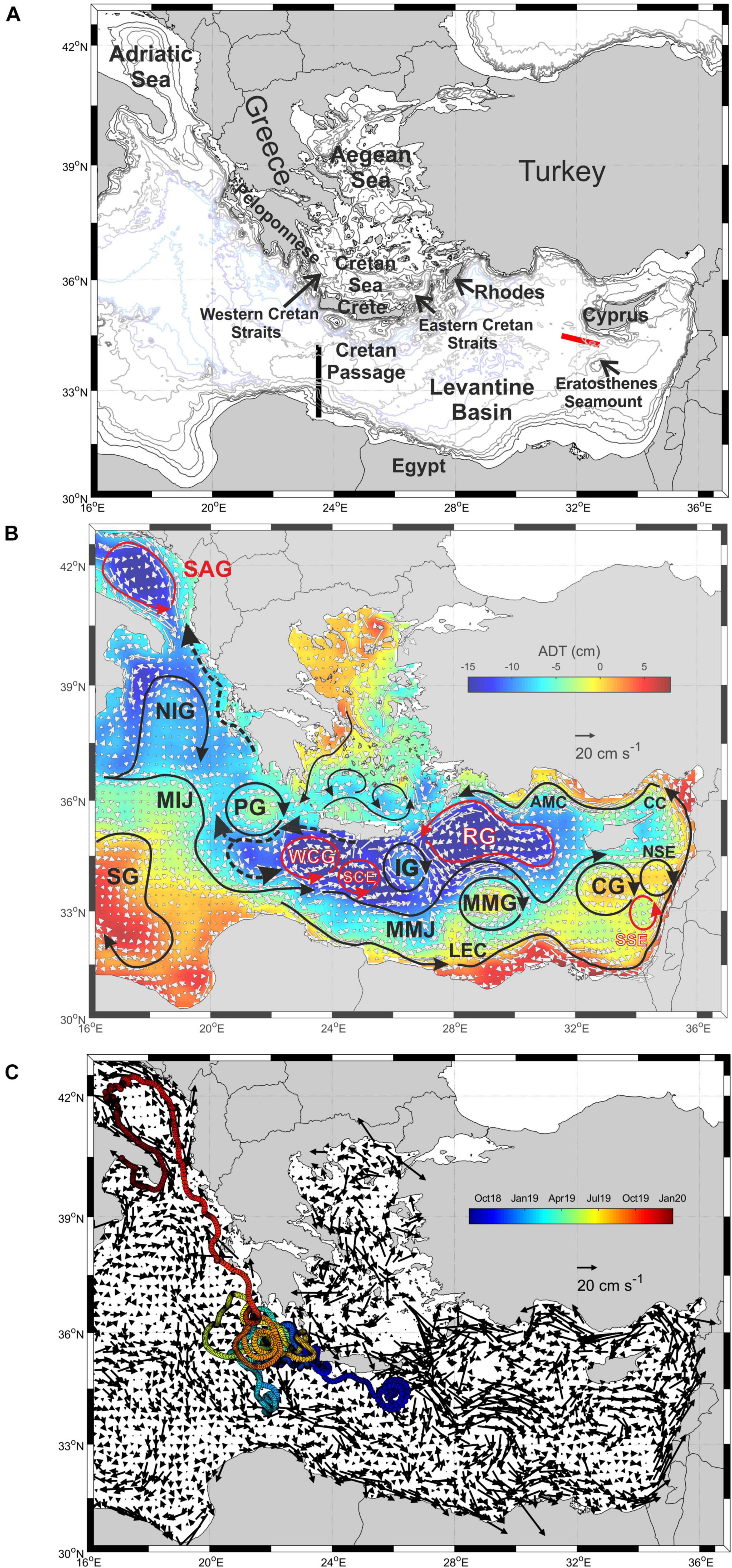
Figure 1. (A) Geography and bathymetry of the EMS (the 200, 600, 1000, 1200, 2000, 2600, 3000, and 3600 m isobaths are showed with thin lines); black and red segments denote the location of transects used in Figure 9. (B) Mean geostrophic currents (white arrows) superimposed on the mean ADT (colors) derived from altimetry in 1993–2019; a schematic representation of the main currents and circulation structures, adapted from Menna et al. (2012; 2019b; 2020) and Mauri et al. (2019), are depicted with black and red arrows. (C) Mean drifter currents in spatial bins of 0.25°× 0.25° in the period 1990–2019 and trajectory of the drifter IMEI 300234065616590 color-coded in time. SAG, Southern Adriatic Gyre; NIG, Northern Ionian Gyre; SG, Sidra Gyre; MIJ, Mid-Ionia-Jet; PG, Pelops Gyre; WCG, Western Cretan Gyre; SCE, Southern Cretan Eddy; IG, Ierapetra Gyre; MMJ, Mid-Mediterranean Jet; LEC, Libyo-Egyptian Current; MMG, Mersa-Matruh Gyre; RG, Rhodes Gyre; CG, Cyprus Gyre; SSE, South Shikmona Eddy; NSE, North Shikmona Eddy; CC, Cilician Current; AMC, Asia Minor Current.

The maps derived from drifter and altimetric data (Figures 1B,C) help to summarize the mean pathways of the surface current field and to identify the main permanent sub-basin scale features. Among these, four anticyclonic gyres dominate the circulation of the EMS: the Pelops Gyre (PG), the Ierapetra Gyre (IG), the Mersa-Matruh Gyre (MMG), and the Cyprus Gyre (CG). Note that, in this work the Mediterranean coherent structures driven by wind and/or topography and located in a fixed geographical area are called gyres, whereas the structures driven by the instability of strong coastal currents that frequently changes their location and lifetime are named eddies, following the indications of Schroeder et al. (2012). The main anticyclones of the EMS are classified as gyres because they are permanent structures forced by wind or generated by interaction between currents and bathymetry. They can somewhat change their position and size at interannual scales (they are not stationary), but are still confined in the same geographical area (i.e., the PG is located southwest of the Peloponnese; the IG southeast of Crete; the CG south of Cyprus; the MMG is squeezed among the Egyptian coast, the IG and the RG) and do not considerably change their position.

The main anticyclonic gyres of the EMS incorporate the Levantine Intermediate Water (LIW), making it sink and affecting its flow into all the Mediterranean basins at intermediate depths (Würtz, 2010). These structures are also characterized by the larger Mixed Layer Depth (MLD) during winter months compared to the whole EMS (with the exception of the cyclonic Rhodes Gyre – RG – where, convection phenomena deepen the MLD by up to 1000 m; Gertman et al., 1994), impacting the primary productivity and the consequent biological activities (see Figure 1 of D’Ortenzio et al., 2005). The deepening of the mixed layer in the wintertime is usually associated with a strong decrease in surface chlorophyll-a (Lavigne et al., 2018) but, on the other hand, this deep mixing can also refill the near-surface nutrient stocks, as recently suggested by Dufois et al. (2016). Condie and Condie (2016) show that both cyclonic and anticyclonic ocean features have the potential to retain and support planktonic communities over many generations. Conditions inside anticyclones are likely to favor upwardly motile plankton.

The anticyclonic structures can play an important role in the transport and retention of marine litter. As recently discussed by Brach et al. (2018) in a comparative analysis between cyclonic and anticyclonic eddies, the latter shows a much stronger capability to entrap litter particles, due to the water convergence in their interior. More specifically, Ramirez-Llodra et al. (2013) show an accumulation of plastic debris on the sea floor in the area of the IG compatible with the gyre-induced process. The measurements of plastic concentration describe a patchy plastic distribution in the Mediterranean Sea related to the variability of the surface circulation (Cózar et al., 2015); major concentrations in the Levantine Basin (Zambianchi et al., 2017; Menna et al., 2020) coincide with the areas marked by the main anticyclonic gyres (see Figure 2 of Cózar et al., 2015).

FIGURE 2

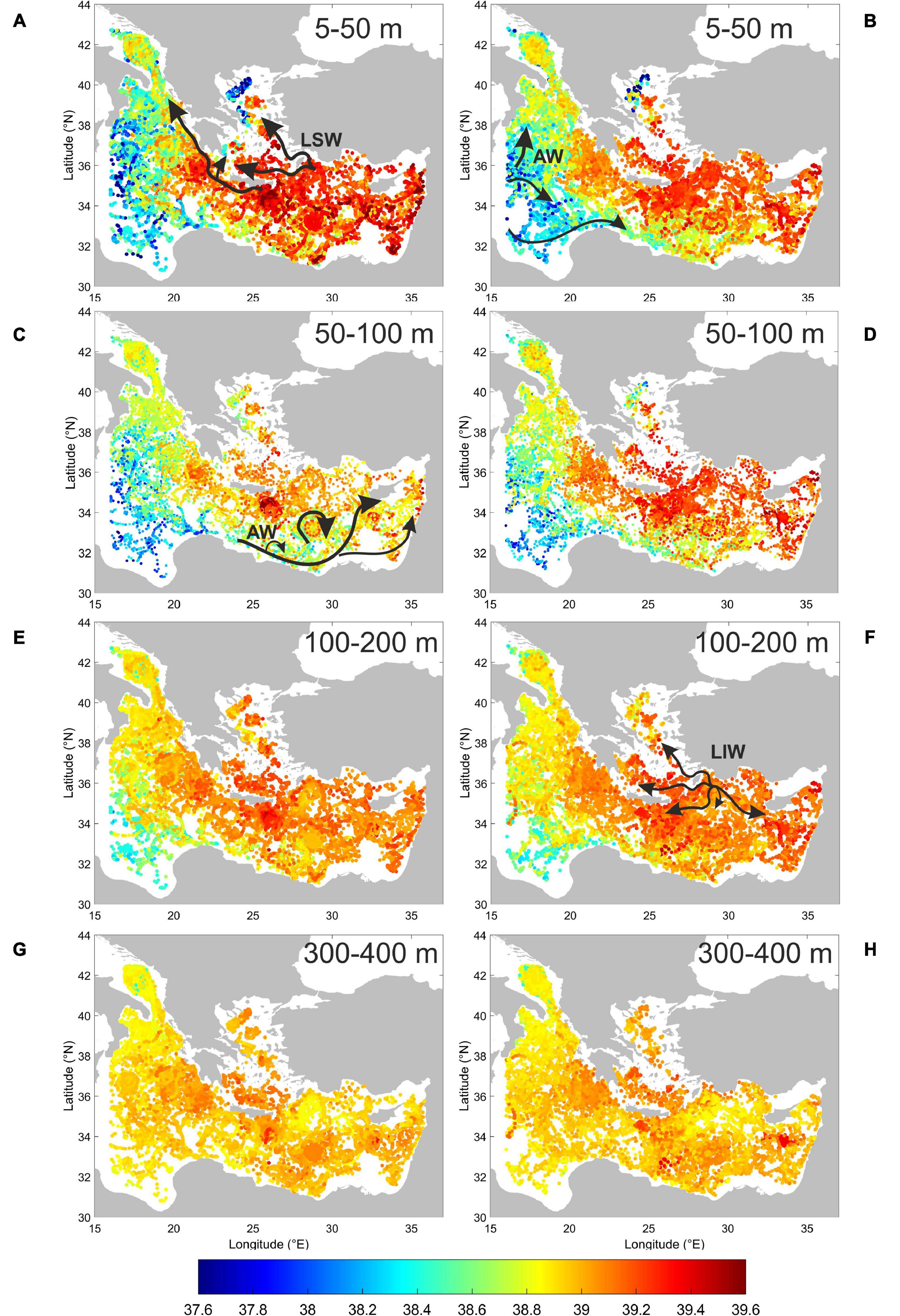
Figure 2. Horizontal scatter plots of mean salinity derived by float in the 5–50 m (A,B), 50–100 m (C,D), 100–200 m (E,F), 300–400 m (G,H) layers during summer/fall (left panels), and winter/spring (right panels) over the period 2003–2019. Black arrows in panel (A,B,C) show the pathway of the AW and LSW adapted from Malanotte-Rizzoli et al. (1997), Hamad et al. (2005); Millot and Taupier-Letage (2005); black arrows in panel (F) show the pathway of the LIW adapted from Hayes et al. (2019).

This article focuses on two out of four main anticyclones of the EMS, the PG and the CG. The PG is located on the eastern side of the northern Ionian Sea, southwest of the Peloponnese coast (Figure 1B). It is a sub-basin scale feature (diameter of ∼ 120 km; Pinardi et al., 2015) forced by the Etesian winds (Ayoub et al., 1998; Mkhinini et al., 2014; Menna et al., 2019b), which extends from the surface down to 800–1000 m depth (Malanotte-Rizzoli et al., 1997; Kovačević et al., 2015). In the late summer/fall the Etesian winds amplify their acceleration and the wind shear in the region of the western Cretan straits (Mkhinini et al., 2014), therefore larger anticyclonic vorticities are observed during these months in the surface layer of the PG region (see Figure 4 of Menna et al., 2019b). At interannual scales, the internal forcing of the Ionian Basin and the outflow of dense waters from the Aegean Sea can influence the variability of the PG (Menna et al., 2019b). Downwelling processes in the core of this gyre are observed and described by Malanotte-Rizzoli et al. (1997); these phenomena affect the thermohaline properties of the Levantine Surface Water (LSW) and of the LIW layers. The PG contribute to the transport of the LIW toward the Adriatic Sea along the eastern Greek coastline (Malanotte-Rizzoli et al., 1997, 1999).

The CG is a dynamical feature located southwest of the Cyprus coast, characterized by seasonal and interannual variability in shape and dimension (Zodiatis et al., 2005; Menna et al., 2012; Mauri et al., 2019). This sub-basin gyre alternates periods of high eddy kinetic energy (larger than 200 cm²s^–2) and diameter of ∼ 100 km with periods in which it extends eastward, merging with the Northern Shikmona Eddy (NSE) (Menna et al., 2012; Mauri et al., 2019) and forming a large anticyclonic structure with a diameter of 250–300 km (Menna et al., 2012). The CG is probably generated by the interaction between the currents and the topography in the region of the Eratosthenes seamount (Gerin et al., 2009) and extends from the surface down to 400 m depth (Zodiatis et al., 2005). During winter, the inner part of the CG is characterized by homogeneous salty water (39.2) down to 400 m depth and by downward doming of the LIW (Mauri et al., 2019). In fall the water column inside the CG shows a strong vertical stratification, with the presence of warm and salty LSW near the surface down to 40 m, the AW just below the LSW (50–100 m depth) and the LIW between 100 and 400 m. The isopycnals are characterized by an upward bending over the high salinity lens and a downward bending below it, typical of an anticyclonic eddy (Mauri et al., 2019). Below 400 m, and therefore below the signature of the CG, there is the Levantine Deep Water (LDW) (Mauri et al., 2019).

In this article, in-situ data collected by autonomous instruments (drifters and Argo floats) are used, in conjunction with altimetry, wind and MLD products, to provide a comprehensive view of the surface and sub-surface features of the EMS, with particular focus on the PG and CG anticyclones. The vertical structures, hydrological characteristics, seasonal and interannual variability, water mass sinking and vertical mixing inside the anticyclones are delineated using the profiles of the Argo floats entrapped for long periods (months or years) inside the selected structures. New insights on the role of the anticyclones of the EMS in modulating the main currents and the exchange of the water masses in the whole basin are suggested and discussed. To our knowledge, this is the first time that the vertical structure of the aforementioned anticyclones is studied in such detail and with such a temporal extension, describing their surface dynamics, the water masses involved and the mixing processes that take place within them.

Data and Analysis

Drifter Data

The drifter tracks used in this work were selected from the OGS Mediterranean drifter dataset (Menna et al., 2017) which cover the period 1990–2019. Drifter data were retrieved from the OGS own projects, but also from databases collected by other research institutions and by international data centers (Global Drifter Program, SOCIB, CORIOLIS, and MIO, etc.). The drifter sampling interval ranges from 6 h to 5 min, depending on the drifter design, the year of manufacture and the instrument positioning system. Drifter data were processed with standard procedures (editing and interpolation; Menna et al., 2017, 2018). In particular, we used a 36-h low-pass filter to remove tidal and inertial frequencies; then, we interpolated the drifter tracks every 6 h.

The interpolated sub-sampled data were grouped into 0.25°× 0.25° bins and pseudo-Eulerian statistics were computed following the method detailed in Poulain (2001) and Thomson and Emery (2001). The pseudo-Eulerian statistics correspond to the near-surface currents between 0 and 15 m depth.

Altimetry Data

The daily (1/8° Mercator projection grid) Absolute Dynamic Topography (ADT) and correspondent Absolute Geostrophic Velocities (AGV) derived from altimeter and distributed by CMEMS (product user manual CMEMS-SL-QUID_008-032-051) were considered. The ADT was obtained by adding the sea level anomaly to the 20-years synthetic mean estimated by Rio et al. (2014) over the 1993–2012 period.

The mean map of ADT and AGV were computed over the period 1993–2019 in bins of 0.25°× 0.25°, in order to be comparable with the drifter-inferred velocity map. Mean maps of ADT and AGV were also computed over the periods (months or years) in which selected floats were entrapped inside the PG and CG (Table 1). These maps help to confirm the presence of the floats inside the studied structures (by comparing the floats trajectory and the concurrent altimetry data; see for example Figure 3A) and to define the surface extension and the strength of the gyres.

TABLE 1

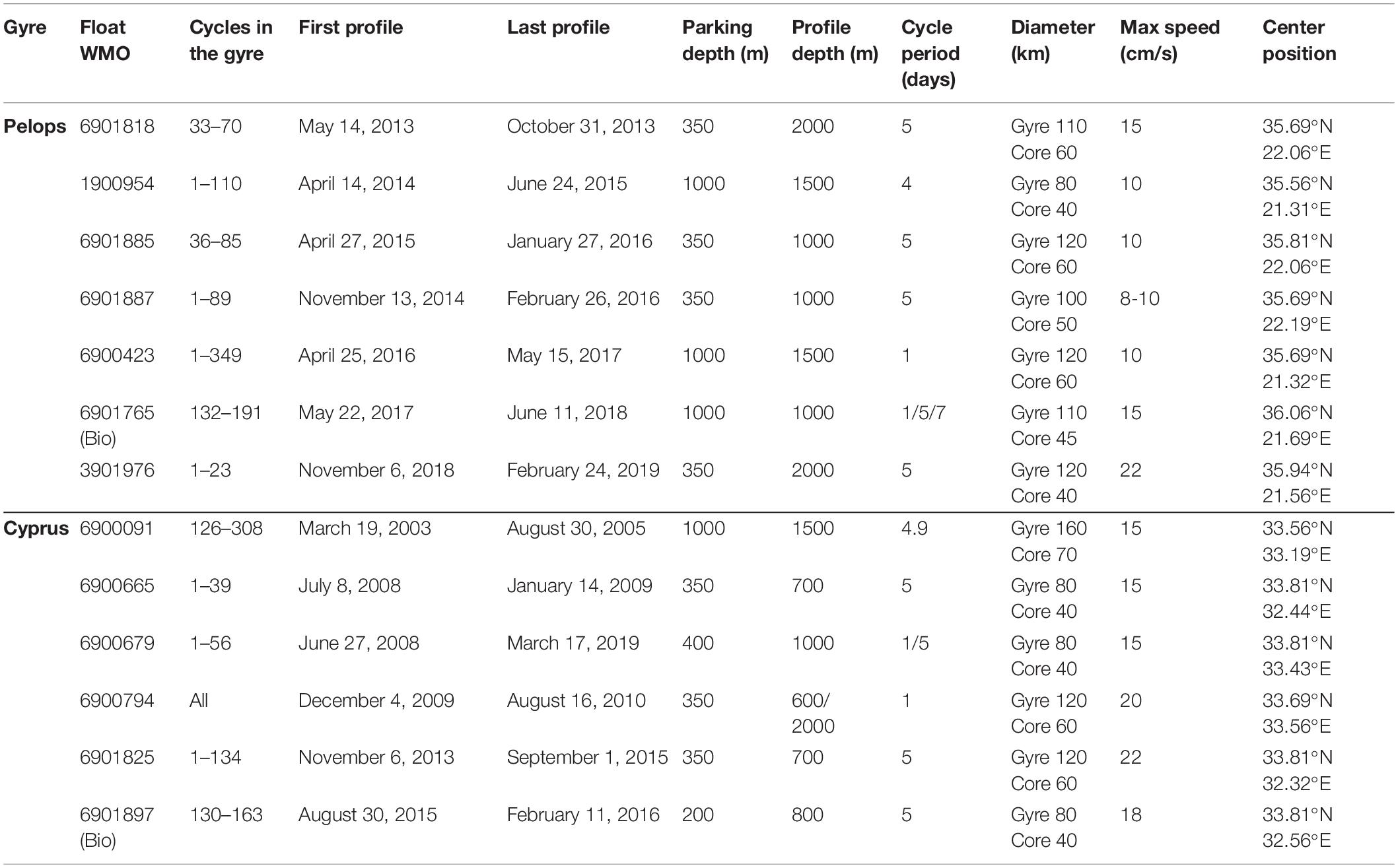
Table 1. List of selected Argo float profiles with dates and positions of the first and the last profile considered in this work, parking and profiling depths, and the cycle period of each instrument. Surface gyres centers, diameters, and maximum speeds are derived from altimetry data.

FIGURE 3

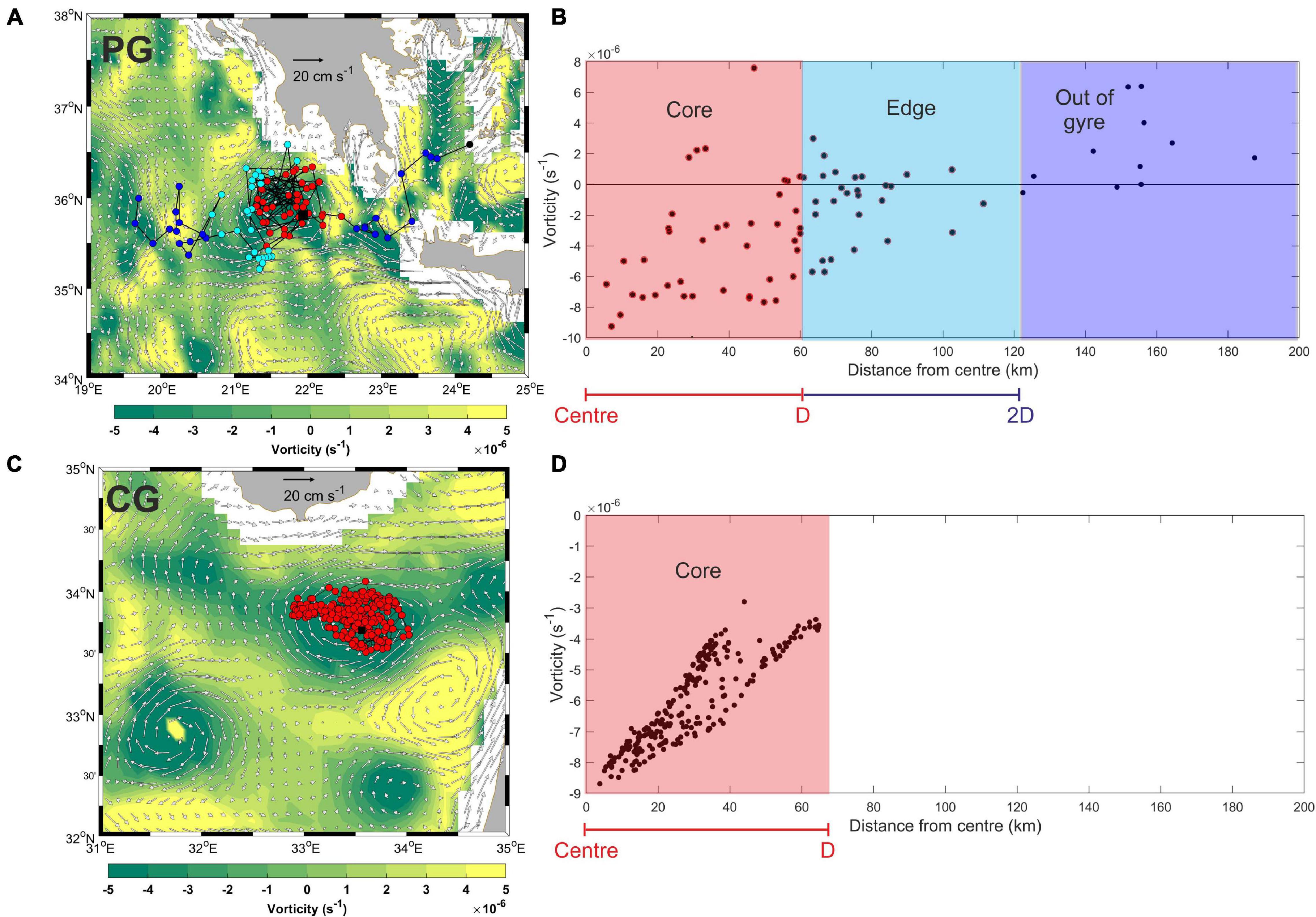
Figure 3. Map of the trajectory (black line) and profile positions (colored dots) of the floats WMO 6901885, entrapped in the PG (A), and WMO 6900794, entrapped in the CG (C), superimposed on the concurrent mean maps of relative vorticity (background color) and AGV (white arrows). The centers of the gyres are represented by black squares. Vorticity values related to each profile versus the distance from gyre center obtained for the float WMO 6901885 in the PG (B) and for the float WMO 6900794 in the CG (D).

FIGURE 4

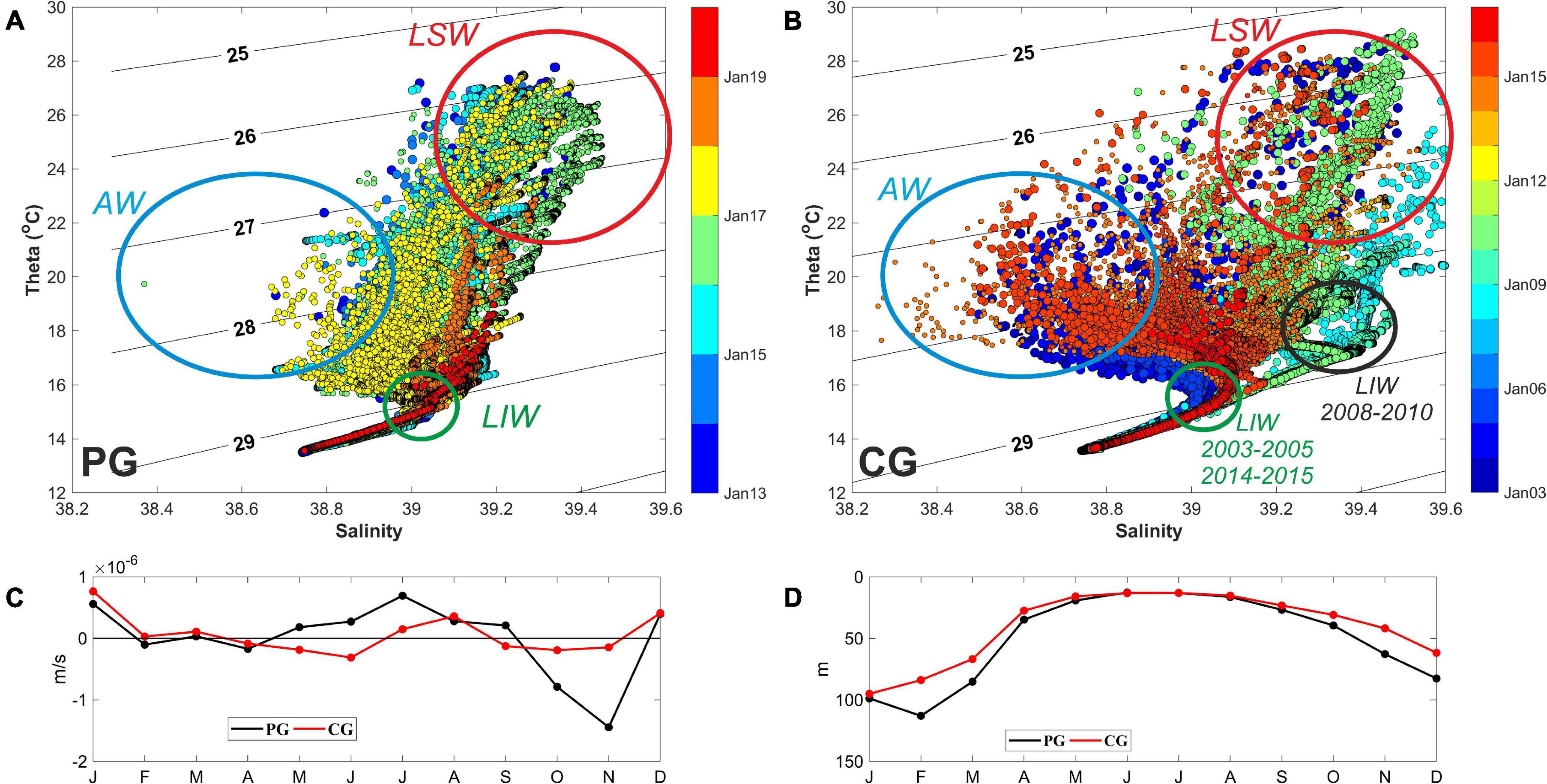
Figure 4. θ/S diagrams of the profiles sampled in the (A) PG and (B) CG colored by the time. The location of the main water masses in the diagrams are highlighted with colored ellipses. Annual evolution of the Ekman pumping (C) and MLD (D) estimated in the period 2007–2019.

The AGV fields were also used to estimate the relative vorticity (ζ), defined as the vertical component of the velocity field curl, as follows:

$$\mathrm{\zeta }=\frac{\partial V}{\partial x}-\frac{\partial U}{\partial y};(1)$$

where, U and V are the velocity components. The resulting current vorticity fields were used to define the coordinates of the gyres center and to select the float profiles collected inside the structures (more details can be found in section “Float Data and Analysis”).

Wind Data and Ekman Pumping Estimation

Wind velocity gridded data (W, with a spatial resolution of 31 km and a temporal resolution of 12 h) were downloaded from the ECMWF ERA5 global atmospheric reanalysis. Eddy induced Ekman pumping, associated with the spatial variation of wind-stress, was calculated from the curl of the wind stress (τ) as: w_EK = curl(τ/ρ⋅f), where, w is an estimate of the vertical velocity, ρ is the density of the water, here considered ρ = 1028 kg⋅m³, and f is the Coriolis parameter that is variable with latitude and in the region of study is ∼ 10^–4 rad⋅s^–1. The mean annual cycle of the Ekman pumping was extracted in the region of the PG (35°−36−5°N, 20.5°−22.5°E) and CG (33.5°−34.5°N, 32−34.5°E). Positive values of w_EK are associated with upward vertical velocities (upwelling), whereas negative values of w_EK indicate downward flow (downwelling).

Mixed Layer Depth

The MLD climatology used in this article¹ is described in Holte et al., 2017. It was computed using Argo profiles and a hybrid method (Holte and Talley, 2009). The climatology incorporates over 2,250,000 Argo profiles (through December 2019) producing a representative annual cycle of monthly mixed layer properties. The climatological values of MLD were extracted and averaged in the areas, where, the anticyclones are located (see section “Wind Data and Ekman Pumping Estimation” for the geographical limits of the anticyclones).

Moreover, the MLD was estimated from the individual float profiles selected in the region of the PG and CG, using the method of de Boyer Montégut et al. (2004) and the Gibbs-SeaWater (GSW) Oceanographic Toolbox (McDougall and Barker, 2011). This threshold method uses a temperature difference criterion, for which the MLD is the depth at which temperature changes by a given value with respect to the near-surface reference depth. The temperature difference used in this work is Δt = 0.2°C, as suggested by D’Ortenzio et al. (2005) for the Mediterranean Sea.

Float Data and Analysis

An overview of the salinity distribution in the whole EMS is obtained from the horizontal scatter plot of mean salinity derived from the float data in four vertical layers (5–50, 50–100, 100–200, and 300–400 m) over the period 2003–2019 (Figure 2). Such layers are representative of the typical depths of the main surface and intermediate water masses’ distribution analyzed in this work and they were selected according to the knowledge available in literature. The seasonal maps are produced over two extended seasons, selected following Menna et al. (2012, 2020): summer/fall (July–December) and winter/spring (January–June).

The vertical extension and the thermohaline properties of the anticyclonic gyres are analyzed using Argo float vertical profiles of temperature and salinity from the upper 2000 m of the water column (Argo, 2020). In the Mediterranean Sea, the Argo floats are generally programmed to execute 5-day cycles alternating the profiling depth between 700 and 2000 m [see the MedArgo program in Poulain et al. (2007)]. Details about the missions of the floats selected for this work are listed in Table 1.

Among all the available data in the Mediterranean Sea, we selected the segment of the trajectories that correspond to floats entrapped in the PG and CG for a long period (months or years; see Table 1), using the concurrent altimetry data. The floats selected move inside the structures, more or less close to the center, describing an anticyclonic trajectory (Figures 3A,C). The profiles selection was then refined by using the mean vorticity fields concurrent with the periods in which the float transits and/or is trapped in the structure. The gyre center is defined as the point, where, the local minimum of vorticity field is observed (black square in Figures 3A,C); the distance of each float profile from the center is computed and the vorticity field is interpolated at the profile location (Figures 3B,D). The vorticity of an anticyclone is negative near its core, close to zero (slightly positive or negative) along the boundary between its core and its edge, and positive along the edge. Considering this behavior, we selected the distance D from the center at which numerous vorticity values become close to zero, and used this distance to define the core and the extension of the gyre (Figures 3B,D). All profiles with distances less than D from the center are considered in the core of the structure (red dots in Figures 3A,C; dots in the red shaded area in Figures 3B,D); all profiles with distances larger than D and lower than 2D are considered in the edge of the structure (cyan dots in Figures 3A,C; dots in the cyan shaded area in Figure 3B); all other profiles are discarded (blue dots in Figure 3A; dots in the blue shaded area in Figure 3B).

Most of the float profiles used in this work were validated using Delayed Mode Quality Control (DMQC) technique. The strategy adopted for DMQC is widely described in Wong et al. (2003); Böhme and Send (2005), Owens and Wong (2009); Notarstefano and Poulain (2013), and Cabanes et al. (2016). The accuracy of salinity measurements requested by Argo after the DMQC is 0.01. When DMQC data are not available, real-time data are used. The float salinity measurements selected in this article have a high level of accuracy: in each structure we performed a qualitative inter-comparison between the θ-S diagrams of the floats entrapped in the anticyclones (Figures 4A,B). A zoom on the deepest and most uniform part of the water column (>800 m and < 1200 m; not shown) shows that the spread of salinity is within 0.02 at 13.7 θ level over a period of 6 years in the PG (from 2013 to 2019) and 13 years in CG (2003–2016). Moreover, the analysis of the θ-S curve of single floats does not reveal any systematic shift in time of the profiles, suggesting a good behavior of the conductivity sensor. Hence, the above mentioned small variations over such long periods are more likely imputable to a natural environmental variability and confirm the high reliability of the data used.

Vertical mixing events occurring inside the anticyclones are analyzed using an indicator of the water column stability known as Turner Angle (Tu; Ruddick, 1983). Tu gives information on the role of salinity and temperature gradients on the density gradients (Kubin et al., 2019). The types of instability are determined by the signs of the potential density θ and salinity gradients rather than by their absolute values (Meccia et al., 2016). In particular, when |Tu| < 45 the water column is stable; when |Tu| > 90 the water column is unstable with respect to both the temperature and salinity profile. The intermediate range shows two options: −90 < Tu > −45 indicates the conditions for diffusive convection (DC); whereas salt fingering can be expected if 45 < Tu > 90. Double diffusion in the ocean occurs when temperature and salinity effects on density oppose each other, while the stratification is statically stable, and occurs because the molecular diffusivity of heat is nearly two orders of magnitude larger than that of salt (Stern, 1960). If both temperature and salinity increase with depth, the potential energy required to maintain the double diffusive instability is derived from the destabilizing temperature component of density (Bebieva and Timmermans, 2016). This type of double DC is referred to as DC and is associated with a DC staircase (a series of homogeneous layers in temperature and salinity separated by sharp gradients in temperature and salinity). The other type of double diffusion arises when temperature and salinity both decrease with depth (i.e., the salinity component of density is destabilizing) and is associated with salt fingers (SF), or a SF staircase.

An estimation of the flux of the AW perpendicular to the transects depicted in Figure 1A was obtained using the mean climatological density (ρ) values along the transects (derived by float data) and the monthly geostrophic velocity components perpendicular to the transects (v, derived from altimetry). Mass transport is estimated as:

$$F=\iint \mathrm{\rho }v\mathit{d}x\mathit{d}z(2)$$

The horizontal dimension of the transects (dx) is of 55 km. In order to closely monitor he AW transport, the vertical dimension (dz) and the density along the Cretan transect (depicted in black in Figure 1A) were defined over the layer 0–100 m depth, whereas those of the Cyprus Passage transect (depicted in red in Figure 1A) were defined over the layer 50–100 m depth. For this estimate, we used the AGV considering their direction and strength as representative of the surface layer between 0 and 100 m depth. Transects locations and orientations were designed to intercept the main pathways of the AW in the Levantine Basin.

Results

Surface Statistics

The mean maps of ADT, AGV and pseudo-Eulerian drifter velocities in bins of 0.25°× 0.25° are used to depict the surface circulation in the EMS (Figures 1B,C). Qualitatively, the two datasets fit rather well and describe the same morphology (shapes, locations and horizontal extension of the main permanent and quasi-permanent circulation features). A quantitative comparison between the two datasets is out of the scope of this work, but it is interesting to note that quantitative discrepancies are imputable to (i) the wind driven and ageostrophic currents included in the drifter velocity measurement (Poulain et al., 2012), (ii) the spatial and temporal gaps due to the non-uniform drifter density (Poulain et al., 2012), and (iii) the spatial smoothing applied to the satellite altimetry data (Pujol and Larnicol, 2005). More details on the circulation structures (Schroeder et al., 2012) and more extensive comparisons between drifter and altimetry derived currents in the EMS can be found in the literature (Gerin et al., 2009; Menna et al., 2012, 2019a,b, 2020; Poulain et al., 2012).

New interesting features, not yet described in the literature, are depicted with dashed black arrows in Figure 1B. They consist of a northward current that connects the Ionian and the Adriatic Sea moving along the eastern Greek coast and a westward current that connects the Levantine and the Ionian Basin moving from the southern Crete coast, feeding the northern branch of the Western Cretan Gyre (WCG). These features are confirmed by the pseudo-Eulerian statistics derived by drifters in Figure 1C. The trajectory of the drifter IMEI 300234065616590 (colored dots in Figure 1C), deployed southeast of Crete (in the IG) in October 2018, links the above described currents and outlines the potential pathway of the LSW between the Levantine and Ionian – Adriatic seas. Along this path, the PG plays an important role in the recirculation and distribution of the LSW in the western part of the EMS. A direct connection between the Ionian and the Adriatic Sea along the eastern Greek coast was already suggested by Malanotte-Rizzoli et al. (1997) in the intermediate layer (200–600 m depth).

Analysis of Thermohaline Properties

Figure 2 gives an overview of the salinity distribution in the EMS as detected by floats in the period 2003–2019. The AW coming from the west fills the surface layer of the Ionian Sea west of 20°E and enters the Levantine Basin moving along the southern coast (Figure 2B). In the Levantine, the mean depth of the AW increases and its pathway can be followed in the 50–100 m layer (Figures 2C,D). The AW moves with the coastal currents and the MMJ, recirculating within the sub-basin scale and mesoscale structures located along its path (Figures 2C,D). The salty LSW (S > 39.05) is formed in the Levantine Basin during summer/fall and fills the first 50 m of the water column (Figure 2A), in agreement with the observations of Malanotte-Rizzoli and Robinson (2012). The pathway of the LSW described in the literature [marked with black arrows in Figure 2A, adapted from Malanotte-Rizzoli et al. (1997) and Velaoras et al. (2014) shows its intrusion in the Cretan Passage, in the Ionian and Aegean seas Malanotte-Rizzoli et al. (1997); Theocharis et al. (1999), Alhammoud et al. (2005); Velaoras and Lascaratos (2010), and Vervatis et al., 2011)]. The LSW enters the Aegean Sea through the eastern Cretan straits, mainly carried by the Asia Minor Current (AMC in Figure 1B; Kontoyiannis et al., 1999) and bifurcates in a branch that feeds the Cretan Sea moving westward, and a second one that moves towards the north (Zodiatis, 1991, 1993; Theocharis et al., 1993). The largest mean salinity values (up to 39.7) are observed along the eastern Levantine coast and in the IG (Figure 2A). The distribution of the surface salinity during winter/spring gives an indication of the spreading of the LSW in the EMS (Figure 2B). Salty waters are observed in the eastern and northern Levantine, in the southern Aegean and in the southeastern Ionian. Relative high salinity values (S = 38.8–39) are also detected in the north-eastern Ionian and in the south Adriatic seas (Southern Adriatic Gyre –SAG; Figure 2B; see the geographical location of the SAG in Figure 1B), suggesting a northward coastal transport of the LSW carried out by the surface currents along the eastern Ionian coast (Figure 1B). The LSW is one of the preconditioning factors of the LIW formation during winter; the winter cooling increases the density of the surface waters and the LSW starts to mix with the underlying waters down to depths of 200–400 m forming the LIW (Malanotte-Rizzoli and Robinson, 2012). The signal of the LIW with a subsurface salinity maximum, is clearly identifiable between 100 and 400 m in the Levantine Basin (Figures 2E–H); an indication of the LIW pathway is given by the black arrows in Figure 2F, adapted from Hayes et al. (2019). Larger salinity values are observed in the southern Aegean Sea, along the eastern Levantine coast, in the IG and CG regions in the layer of 100–200 m (Figures 2E,F). In the intermediate layer, between 300 and 400 m depth, the salinity maximum is identified in the core of the IG and CG structures (Figures 2G,H).

We selected 7 floats for the PG (664 profiles) and 6 floats for the CG (667 profiles) that spent part of their life inside the structures (Table 1), to cover the widest possible time period and highlight the seasonal and interannual variabilities. The water masses, sampled in the first 2000 m of the water column in the regions of the PG and CG, are shown in the θ/S diagrams of Figure 4 and their thermohaline characteristics summarized in Table 2. The results of Table 2, rather than being an exhaustive classification of the thermohaline characteristics of the individual water masses, are intended to provide their range of thermohaline variability within the different structures. The ranges reported in this article are in agreement with recent results available in the literature for the EMS (see Table 2).

TABLE 2

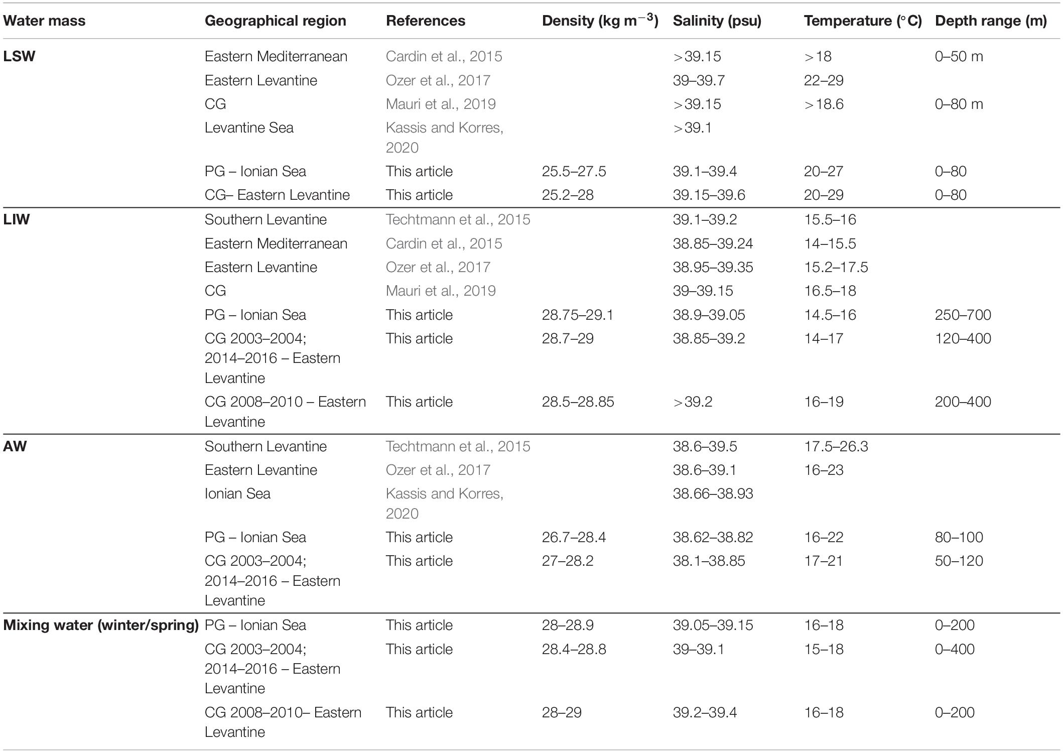
Table 2. Water masses of the EMS and their thermohaline properties inside.

The θ/S diagrams show the presence of three main water masses (Figure 4). The LSW is characterized by the salinity maximum (S > 39.05), potential temperature larger than 20°C and potential densities smaller than 28 kg m^–3 (Figure 4 and Table 2). The AW, characterized by the lowest salinity and potential temperature of 16–21°C, is detected only sporadically in the PG (a few profiles in the area of the θ/S occupied by the AW; Figure 4A). The LIW layer is characterized by potential density larger than 28.7 kg m^–3 and salinity of 38.85–39.2. The LIW sampled in the CG in 2008–2010 is warmer and saltier than that sampled before and after this period, allowing to identify two different LIW “cores” in the CG (Figure 4B). These outcomes are addressed in more detail in sub-section “Pelops Gyre” and sub-section “Cyprus Gyre,” along with an accurate description of the thermohaline properties and mixing.

Figures 4C,D provide an overview of the annual climatology of the atmospheric forcing and MLD in the PG and CG. In the wind-forced PG, the Ekman pumping shows the largest negative values (downward flow) in fall, in concomitance with the strengthening of the Etesian winds, and weak positive ones (upward flow) in spring and summer. The Ekman pumping effect is reduced in the region of CG; this structure is not driven by the wind, indeed the input of the wind stress curl is positive (cyclonic) in this area (see Figure 2 of Amitai et al., 2019). The annual evolution of the MLD is similar for both the gyres, with values smaller than 30 m in the period March-October and increasing values between November and February (Figure 3D). High mean MLD values, larger than 100 m, are observed in the region of the PG in February.

For each gyre, the θ/S diagram and the contour diagram of salinity and turner angle are shown in Figures 5–8. The float profiles selected for each structure are sorted in the figures chronologically according to the periods covered by the data.

FIGURE 5

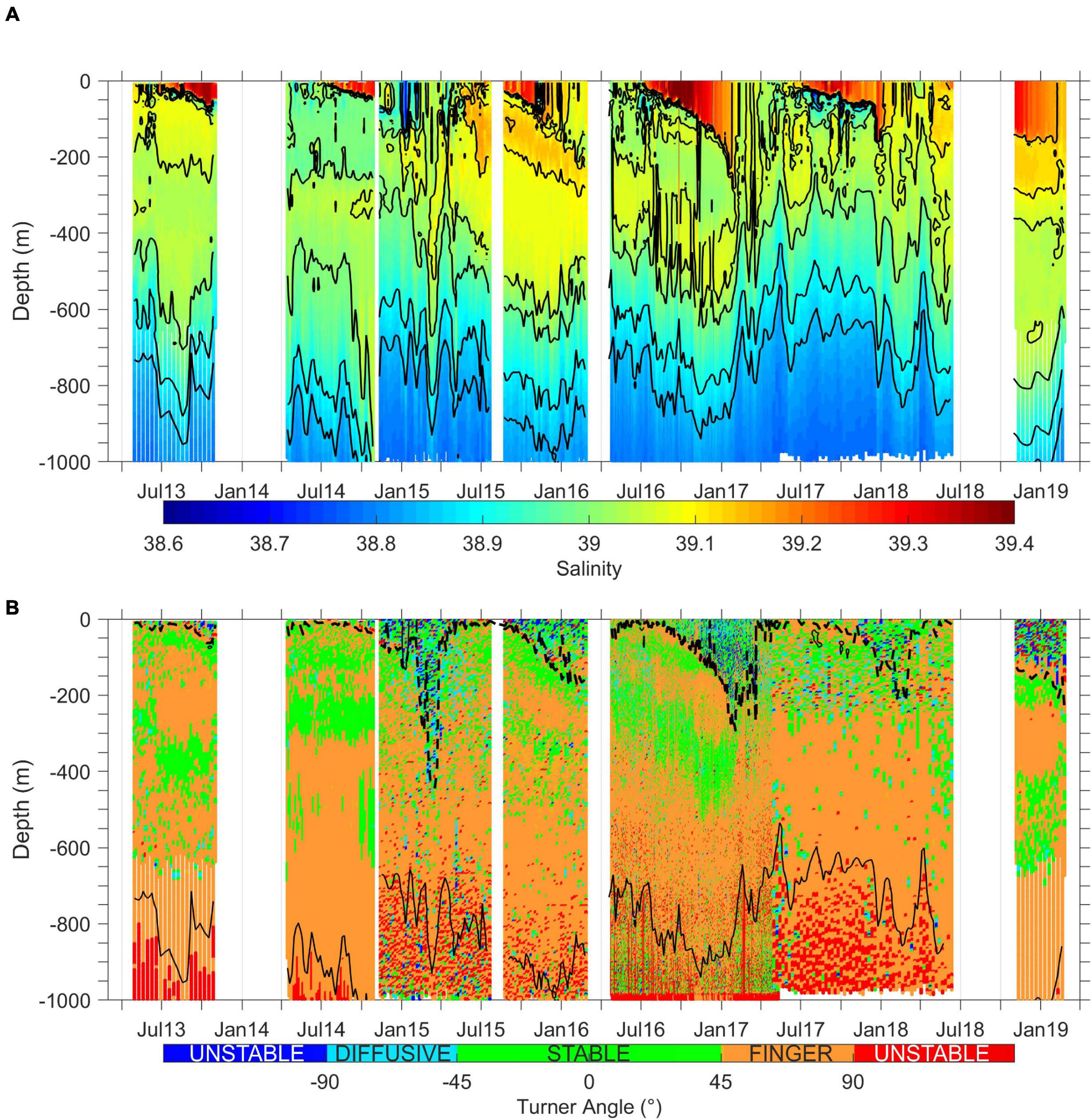
Figure 5. Contour diagrams of the salinity (A) and turner angle (B) versus depth and time for the float entrapped in the PG. Black continuous lines in (A) are the isohalines 38.85, 39, 39.05, and 39.15; black dashed line in (B) is the MLD estimated by float profiles; black continuous line in (B) is the isohaline 38.85.

FIGURE 6

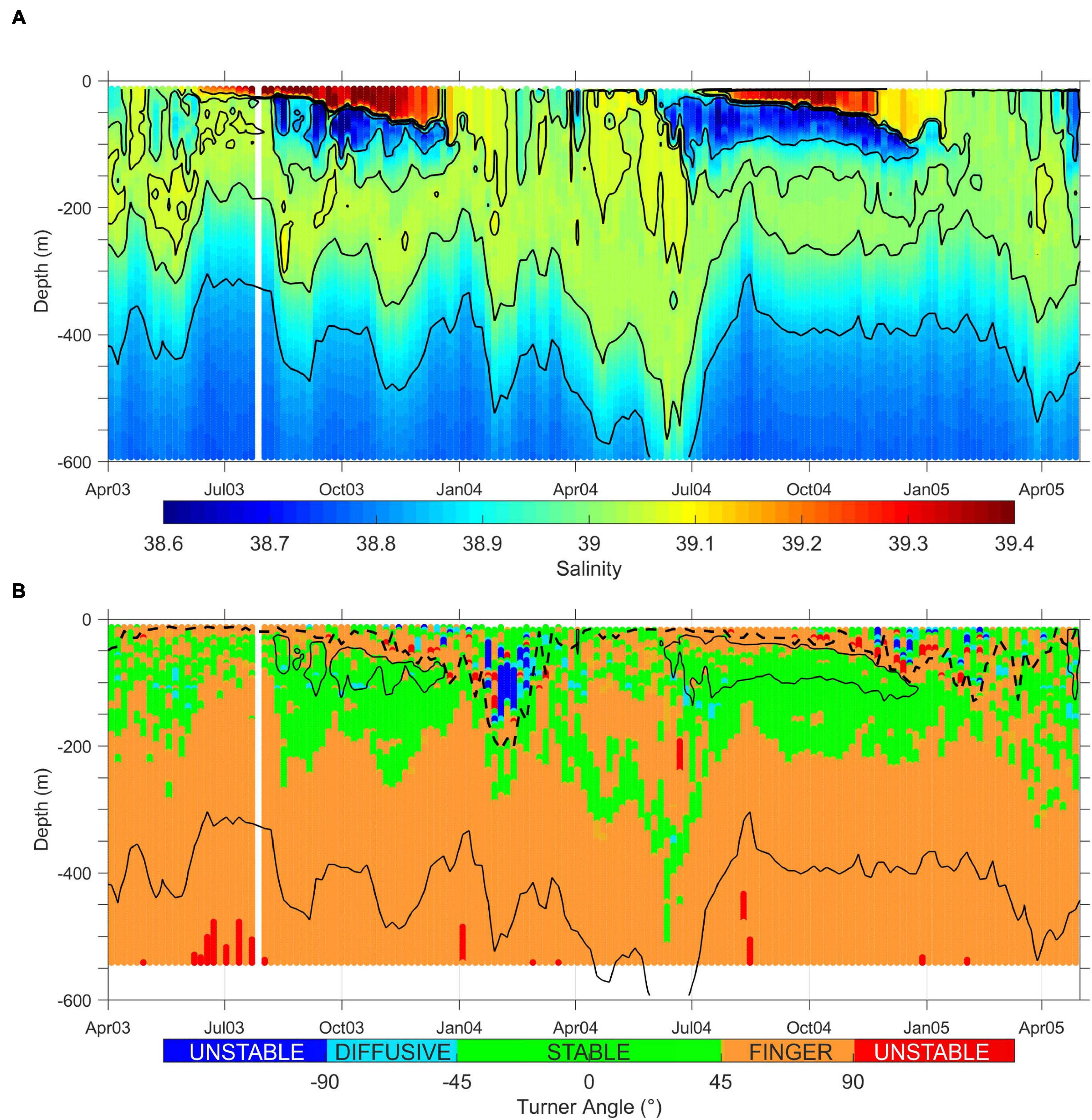
Figure 6. Contour diagrams of the salinity (A) and turner angle (B) versus depth and time for the float entrapped in the CG in 2003–2005. Black continuous lines in (A) are the isohalines 38.85, 39, 39.05, and 39.15; black dashed line in (B) is the MLD estimated by float profiles; black continuous line in (B) is the isohaline 38.85.

FIGURE 7

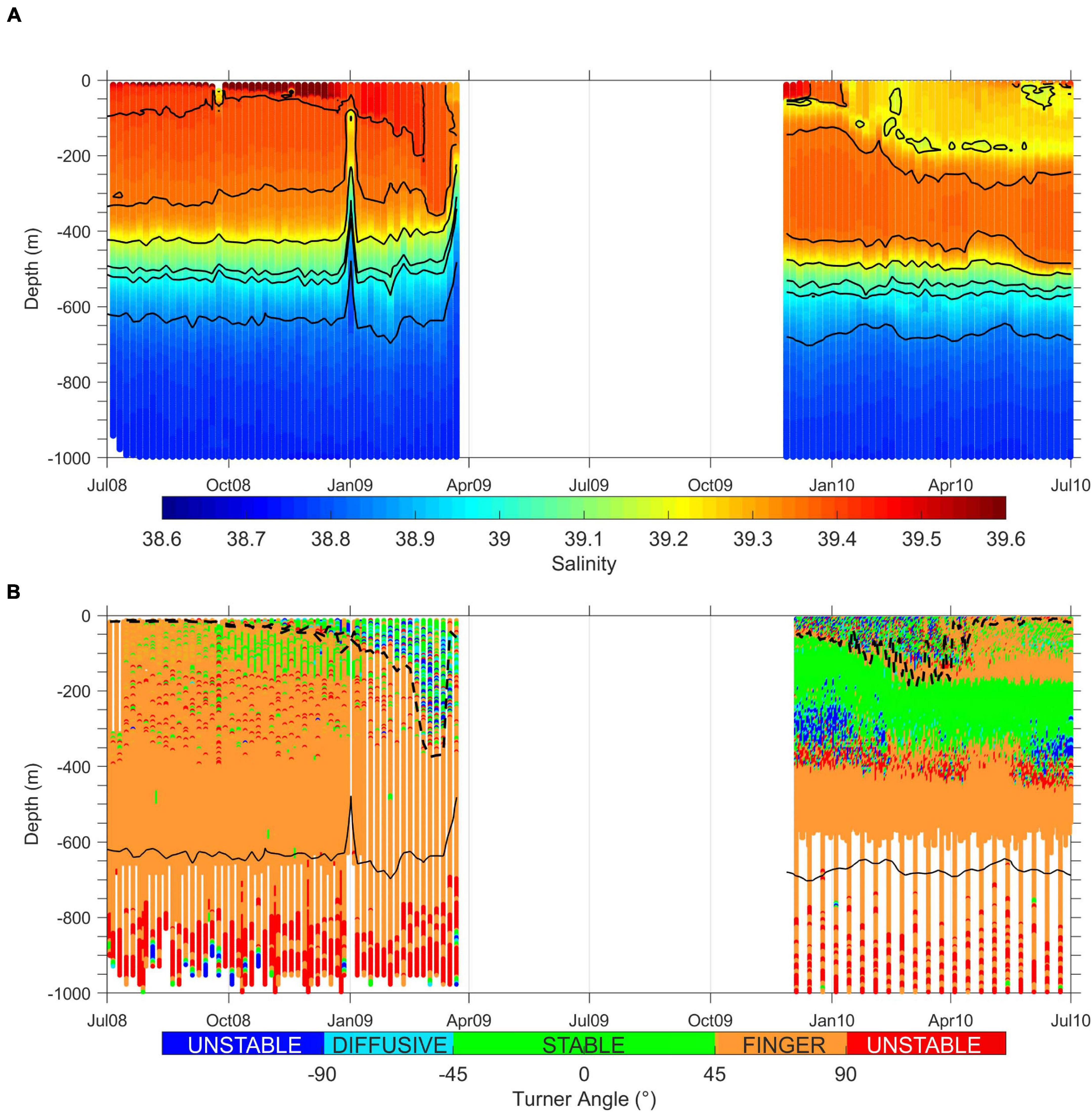
Figure 7. Contour diagrams of the salinity (A) and turner angle (B) versus depth and time for the float entrapped in the CG in 2008–2010. Black continuous lines in (A) are the isohalines 38.85, 39, 39.05, 39.2, 39.35, and 39.4; black dashed line in (B) is the MLD estimated by float profiles; black continuous line in (B) is the isohaline 38.85.

FIGURE 8

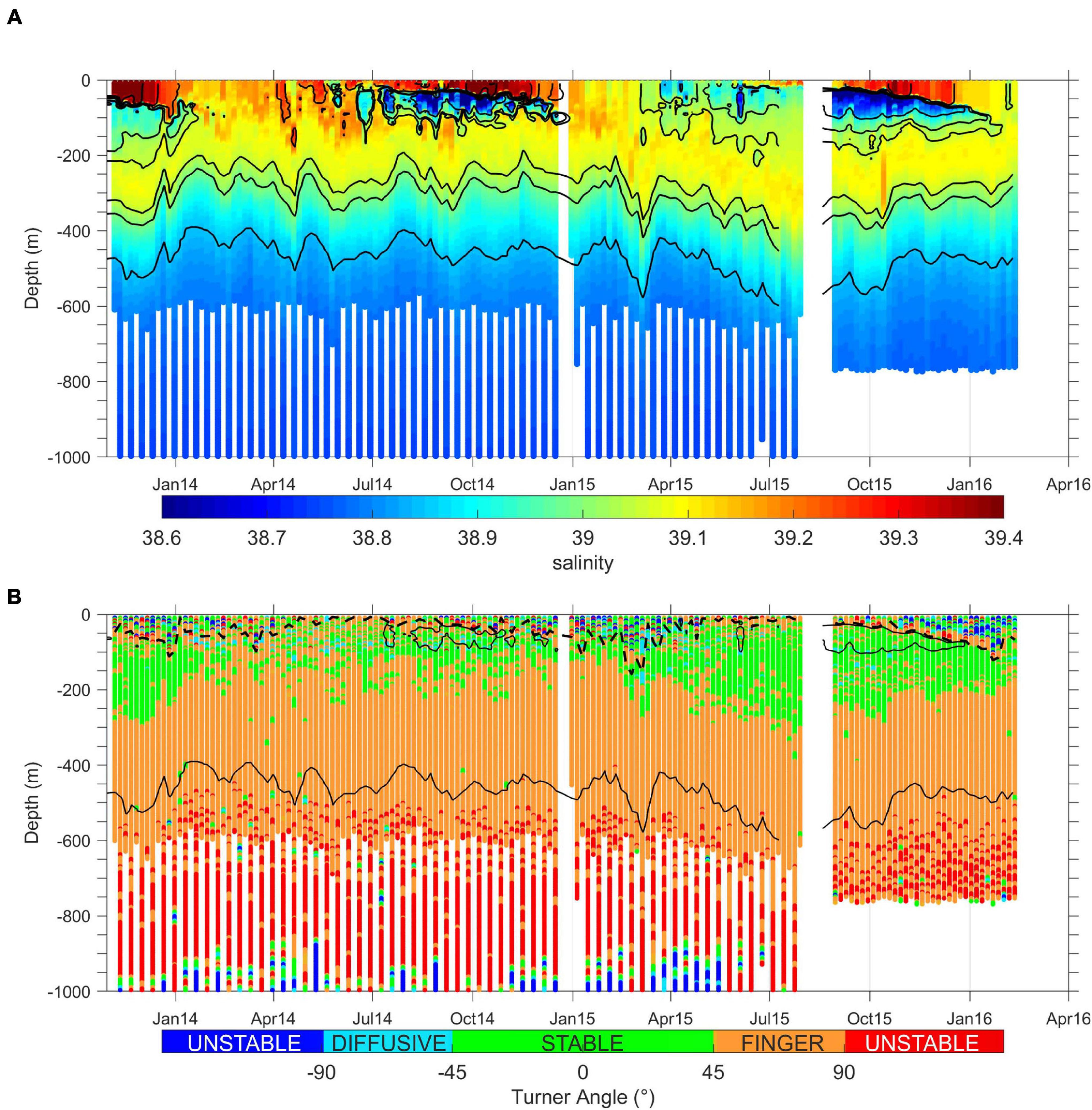
Figure 8. Contour diagrams of the salinity (A) and turner angle (B) versus depth and time for the float entrapped in the CG in 2014–2016. Black continuous lines in (A) are the isohalines 38.85, 39, 39.05, 39.2, 39.35, and 39.4; black dashed line in (B) is the MLD estimated by float profiles; black continuous line in (B) is the isohaline 38.85.

Pelops Gyre

The PG is sampled almost continuously by 7 floats in the period 2013–2019 (Figure 5). The main gaps in the data occur in October 2013–April 2014, February–April 2016, and June–November 2018. The PG center is generally located between 35.5−36.1°N and 21.3°−22.1°E (Table 1) and its vertical extension reaches ∼ 800–900 m depth (Figure 5A; the vertical extension of the PG is indicatively represented by the isohaline of 38.85). The surface dynamics of the gyre, described averaging the ADT and AGV fields concurrent with the float trajectory, define a mean diameter of 80 – 120 km and maximum speeds of 15 cm/s in 2013, smaller than 10 cm/s in 2014–2018 and larger than 20 cm/s in 2019 (Table 1).

In summer/fall (July–October), the upper layer of the PG (50–80 m depth; Figure 5A) is filled by the LSW, characterized by high salinity maximum (S > 39.1), the largest potential temperature and potential densities smaller than 27.5 kg m^–3 (see water mass details in Table 2 and Figure 4A). The AW, characterized by lowest salinity and potential temperature of 16–21°C, enter the PG only sporadically (a few profiles in the area of the θ/S diagram meet the thermohaline characteristics of the AW; Figure 4A). A thin vein of AW is recorded in the structure in summer/fall 2013 and 2017, located below the LSW at 80 m depth (Figure 5A). The LIW layer, characterized by densities larger than 28.75 kg m^–3 and salinities of 38.9–39.05, is generally located between 250 and 450 m; it is deeper (400–700 m depth) for the profiles collected in 2018–2019. In late fall – early winter, the fast decrease of temperature in the saline surface layer of the PG leads to a rapid increase in density (gradual downward bending of the isopycnals and isohalines) with consequent water sink and mixing with waters of the underlying layer. The water mass formed by the winter mixing shows intermediate thermohaline characteristics between the LSW and the LIW (Table 2) and fills the layer between 0 and 200 m during winter–spring seasons in the PG. Under the LIW layer, between 800 and 1000 m, the floats detect the signature of the CIW in the PG (S = 38.85–38.9; σ = 29.1–29.15; Figures 4A, 5A).

The analysis of the water column stability and stratification (Tu), superimposed on the time series of the MLD derived by float profiles, is shown in Figure 5B. The clearest and dominant feature in the water column within the PG is the proneness to double diffusion and in particular to the SF regime (−90 < Tu > −45;orange colored zones in Figure 5B). In July–October, the upper layer of the anticyclone (Figure 5A) is saltier and warmer than the underlying water and, at the interface between these water masses (located just below the signature of the MLD, Figure 5B, and/or the maximum salinity gradient, Figure 5A, at 50–80 m depth), the water column shows a thin layer prone to the SF regime (Figure 5B). Immediately below this layer, approximately between 50 and 150 m, we observe a layer with stable conditions (colored in green in Figure 5B), characterized by homogeneous thermohaline properties, that corresponds to the mixing – produced water. Another layer characterized by stable conditions is located between 250 and 600 m (depth changes over the years), and corresponds to the LIW. Areas located between the two stable layers, as well as those located below the LIW to the whole vertical extent of the PG, are affected by SF. The sensitivity of the Ionian 200–1000 m layer to the SF condition was previously highlighted by Zodiatis (1992) and Kioroglou et al. (2014), by analysing CTD profiles, and by Meccia et al. (2016) using model reanalysis products. In late fall, the MLD starts to increase typically reaching a depth between 150 and 300 m in the period January–March. In 2015, float data show the maximum MLD over the examined period (∼ 440 m depth); the occurrence of this “deep mixing” event is also clearly documented by the contour diagrams of salinity (Figure 5A), potential temperature and potential density (not shown). The part of the water column involved in the deepening of the MLD becomes instable (|Tu| > 90; blue dots in Figure 5B) and thus prone to mixing phenomena. Conditions for SF also occur during mixing events in the layer below the mixed layer. Layers located below the vertical extension of the PG show instable conditions (red and blue dots in the deep layer of Figure 5B), suggesting the occurrence of deep mixing phenomena.

Cyprus Gyre

The CG was sampled by Argo floats intermittently since January 2003. The periods in which data are available are: 2003–2005, 2008–2010, and 2014–2016 (Table 1). The CG center is located between 33.5°N and 33.85°N and 32.4–33.5°E and the gyre extends from the surface to about 400 – 600 m depth (Figures 6–8; the vertical extension of the CG is indicatively represented by the isohaline of 38.85). The surface signature of the gyre shows a mean diameter between 80 and 160 km (Table 1), in agreement with the results of Prigent and Poulain (2017). The maximum surface speeds detected in the periods sampled by floats range between 15 and 22 cm/s, but it is interesting to remind that the CG area is characterized by high variability as a result of its interaction with the MMJ and the South Shikmona Eddy (SSE; located south east of the CG; see Figure 1B). For instance, an extensive analysis, carried out in the CG in February–May 2017 using drifter data, reveals a diameter of 80–100 km and a maximum speed of 50 cm/s (Prigent and Poulain, 2017; Mauri et al., 2019).

The CG presents a strong interannual variability with two main thermohaline patterns. The first pattern is observed in the periods 2003–2005 (Figure 6A) and 2014–2016 (Figure 8A), when the CG shows a seasonal alternation of a homogeneous water column during winter/spring (0–400 m depth) and a stratified condition during summer/fall. The summer/fall stratification is characterized by the following layers: the LSW in the first 50–80 m depth (S > 39.15); a vein of AW between 50 and 120 m depths (S < 38.85); the LIW between 120 and 350–400 m (salinities between 38.85 and 39.1). The second thermohaline pattern occurs in the period 2008–2010, when the CG is filled by a homogeneous layer of salty water (S > 39.2) distributed between 0 and 450 m depth (Figure 7A). In this layer, the thermohaline characteristics remain approximately unchanged over all the seasons without any AW signal. Seasonal intrusion of the LSW with salinity values up to 39.4 are observed in the first 50 m of the water column during summer/fall (Figures 4B, 7A). Winter cooling in 2009 and 2010 favors the sinking of LSW from the surface to 400 m and 200 m depths, respectively (Figure 7A), maintaining the high salinity of the upper homogeneous layer. The thermohaline characteristics of the LIW detected in the CG during 2008–2010 show larger salinities and lower densities compared to the other periods analyzed (Figure 4B).

During the first thermohaline mode (periods 2003–2005, and 2014–2016), in the layer 0–50 m of the water column, the CG shows unstable conditions in late fall/winter and SF conditions in summer/early fall. Stable conditions are observed in the layer between 50 and 200 m (Figures 6B, 8B). Below 200 m, the water column is prone to the SF mode which extends to the whole depth of the gyre. When the winter mixing is sufficiently intense and deep, involving the 0 – 200 m layer (January–March 2004; Figure 6A), the stability condition inside the CG (January–March 2004; Figure 6B) are similar to those observed in the PG: two stable layers are detected at 70–100 m and 200–300 m depths interspersed by a SF layer. The water mass formed by the winter mixing shows intermediate thermohaline characteristics between the LSW and the LIW (Table 2) and fills the first 300–400 m of the water column during winter.

During the second thermohaline mode (period 2008–2010), the water mass produced by winter mixing shows salinities of 39.2 and fills the layer 0–200 m. Stable conditions are observed in the core of the LIW layer (200–400 m depth) and instability at its interface with the underlying layers.

Layers located below the signature of the CG (depths larger than 600 m) show mixing conditions (red and blue dots in the deeper layer of Figures 7B, 8B), as already observed in the PG. These layers are filled by the LDW, formed in the core of the RG and recently described in Kubin et al. (2019) (θ = 13.7–14.5°C, S = 38.8–38.9).

Discussion

The anticyclones of the EMS play a crucial role in the distribution of the surface and intermediate water masses of Levantine origin, both inside the Levantine Basin and in the whole EMS. In this article, float data available within two structures, the PG and CG, were analyzed in detail. The PG is involved in the transport of the LSW and of the LIW toward the northern Ionian and south Adriatic seas (Figure 2). The LSW turns anticyclonically in the upper layer of the PG before joining the weak, northward surface coastal current described by the mean maps of altimetry and drifter data (Figures 1B,C). This current is northward oriented, whatever the circulation mode of the NIG (cyclonic or anticyclonic; see Figure 2 of Menna et al., 2019b and Notarstefano et al., 2019). The LSW transported by the coastal northward current along the western Greek coast could be responsible for the near-surface salinity maximum observed by Kokkini et al. (2018, 2020) in the South Adriatic Pit (SAP) during 2015–2016, by Kassis and Korres (2020) in 2005–2010 and by Mihanovic et al. (2021) in 2017. These authors describe an anomalous salinity pattern in the SAP, where, the maximum is located in the near-surface layer (around 100 m depth) instead of in the intermediate layer occupied by the LIW. These salty water masses in the near-surface layer, with a salinity of 38.9 (Kokkini et al., 2020), can be ascribed to an intrusion of the LSW, of Aegean or Levantine origin, further modified during its journey toward the south Adriatic.

In summer, the effect of surface temperature warming combined with the evaporation rates produces the formation of the LSW in the Levantine Basin (Hecht et al., 1988). This water mass strongly influences the seasonal variability of the analyzed anticyclonic gyres, affecting the water column stratification in summer/fall and the mixing events in winter. The LSW, entrapped in the anticyclones in summer/fall, fills the first 50/80 m of the water column, with a wider range of salinity values in the CG (S = 39.15–39.6; Figure 4B) and lower salinities in the PG (S = 39.1–39.4; Figure 4A). In summer/fall the CG frequently shows, below the salinity maximum of the LSW, a salinity minimum ascribable to the AW, generally located between 50/80 and 150 m (Figures 6, 8). This sub-surface layer of AW characterizes only sporadically the vertical structure of the PG (Figures 4, 5). The layer between 50/80 and 200 m depth in the PG and CG is filled by a water mass with intermediate thermohaline characteristics between the LSW and the LIW (Figures 4–8). This water mass is the result of the mixing phenomena occurring in winter.

In terms of water column stability, the PG and the CG are strongly characterized by the SF regime alternated to winter mixing events (Figures 5–8). The sensitivity of the Ionia Sea to the SF is attributed to the hot and saline LIW waters filling the basin from 200 to 400 m at various places, overlying the less saline and colder resident waters (Zodiatis, 1992; Onken and Brambilla, 2003; Kioroglou et al., 2014). This condition also occurs in the PG not only in the layer below the LIW, but also in the subsurface layer (50–80 m depth) at the interface between the saltier and warmer LSW and the underlying water (Figure 5). In the layer below 1000 m, the water column of the Ionian Basin is considered stable with some sporadic shifts toward the SF or DC regimes caused by temporary intrusions of waters with different thermohaline properties (Kioroglou et al., 2014; Meccia et al., 2016). This condition does not occur in the PG, where, the layers located below its vertical extension (red and blue dots in the deep layer of Figure 5B) show instability down to 2000 m (not shown), suggesting the occurrence of deep mixing phenomena in this layer. In the Levantine Basin double diffusion processes are linked to the SF regime in the first 1000 m depth (Meccia et al., 2016; Kubin et al., 2019) and to the DC at larger depths (Meccia et al., 2016). In the interior of the CG, the SF condition is clearly predominant in the layer below the LIW (Figures 6–8), whereas the mixing conditions dominate the layer below the signature of the CG (depths larger than 600 m; red and blue dots in the deeper layer of Figures 7B, 8B).

The gradual deepening of the MLD and the consequent downward doming of the isohalines, is usually observed in November–January in the PG and in January–March in the CG (Figures 5–8). The mixing generally involves the first 200 m of the water column, but occasionally can affect both the LSW and the LIW layers, as in winter 2015 in the PG (Figure 5A). The water mass formed by the winter mixing fills the surface layer of the gyres between 0 and 400 m during winter–spring seasons.

The CG presents two different behaviors in the periods analyzed. In 2003–2005 and 2014–2016, it is characterized by seasonal variability with the alternance of a homogeneous water column during winter/spring (0–400 m depth), and a stratified condition during summer/fall. The AW, observed inside the CG in the layer of 50–120 m depth (S < 38.85), during winter mixes with the overlying LSW and favors the dilution of the water formed during the mixing events (Figures 6, 8). Otherwise, in the period 2008–2010 the CG shows a slight seasonal variability and it is filled by a homogeneous layer of salty water (S > 39.2), distributed between 0 and 400 m depth. Under this condition, winter cooling favors the sinking of LSW from the surface down to 400 m depth (Figures 2G,H, 7), helping to maintain the high salinity of the upper homogeneous layer. The signal of AW is not detected in the CG in the period 2008–2010, therefore the winter mixing phenomena occur between two highly saline water masses (the LSW and LIW), supporting the production of a saltier mixing water and deepening the depth of the LIW layer (Figure 7 and Table 2). The thermohaline differences observed between these periods can be related to the quasi-decadal reversal of the surface circulation in the NIG, from anticyclonic to cyclonic and vice versa. This connection is supported by the timeseries of the mass transport (Figure 9) estimated through two transects of the EMS: transect located at Cretan Passage (depicted in black in Figure 1A) intercepts the flow of AW from the Ionian toward the Levantine in the first 100 m of the water column (see the AW partway in Figures 2B,C; positive values of mass transport indicate an eastward flow); transect located southwest of Cyprus (depicted in red in Figure 1A) intercepts the inflow of AW transported by the MMJ in the CG region in the layer of 50–100 m depth (Figures 1B, 2C; positive values of mass transport indicate a northeastward flow). The fluctuations of the time series of mass transport at Cretan Passage are in line with the quasi-decadal NIG reversals, with the strengthening of the AW transport toward the Levantine Basin during cyclonic circulation modes (emphasized in light gray in Figure 9) and its weakening during the anticyclonic circulation modes. In the periods 2003–2005 and 2014–2015, the NIG is cyclonic, favoring the flow of the AW toward the Levantine (larger mass transport at Cretan Passage; Figure 9) with a resulting decrease in salinity of the LSW and LIW layers (Civitarese et al., 2010; Ozer et al., 2017; Menna et al., 2019b). In the period 2008–2010 the NIG is instead anticyclonic, favoring the enhanced flow of the low saline AW toward the northern Ionian and South Adriatic seas and its reduction toward the Levantine Basin (reduced mass transport at Cretan Passage; Figure 9), with a consequent salinity increase in the Levantine (Civitarese et al., 2010; Ozer et al., 2017; Menna et al., 2019b). In transect located south-west of Cyprus, although the quasi-decadal variability is less evident, minima values of the AW transport are observed during anticyclonic periods; the absolute minimum of the time series is observed in 2007–2008, concurrently to the disappearance of the AW signal in the CG (Figure 7). This mechanism can explain the recent result of Hayes et al. (2019), which detect the deepest depth of the LIW layer in the Levantine Basin just in the region of the CG, using glider and float data in 2002–2014. LIW layer depths larger than 500 m estimated by Hayes et al. (2019) are in agreement with those estimated in this article over the period 2008–2010 (Figure 7). It is interesting to add that the floats of 2008–2010 are characterized by a prevalence of profiles in the center of the structure, while those from the periods 2003–2005 and 2014–2015 move over a larger area that includes both the center and the border of the gyre. The presence of a high salinity core in the CG is a characteristic already observed from glider data collected in fall 2016 (Mauri et al., 2019).

FIGURE 9

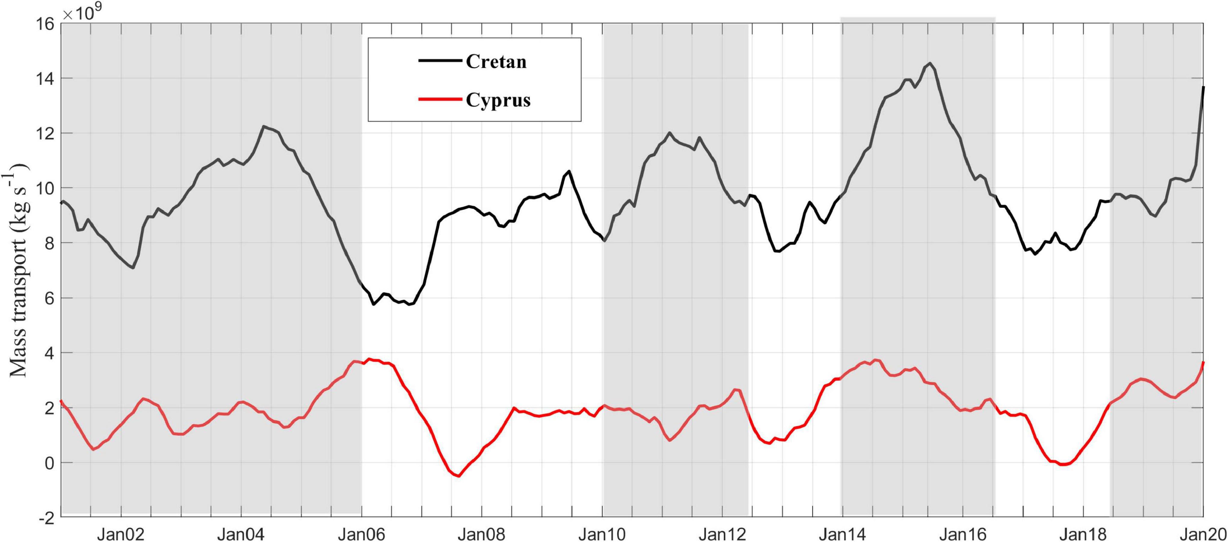
Figure 9. Timeseries of the Mass transport across transects shown in Figure 1A in the period 2001–2019: the black transect located in the Cretan Passage and the red transect located southwest of Cyprus. Periods with cyclonic NIG are emphasized in light gray. Positive values of the mass transport indicate eastward/northeastward flows through the Cretan/Cyprus transects, respectively.

The results on the water column stability in the deeper layer, below the anticyclones signature, suggest the role of these structures in transporting energy, slat and heat from the surface layer to the bottom promoting deep mixing (Figures 5–8 panels B). These observations are consistent with the model studies on the role of coherent anticyclones in the penetration of available potential energy toward the deeper ocean layers, with the consequent increasing of the mixing at depth (e.g., Koszalka et al., 2010). This deep mixing can also refill the near-surface nutrient stocks, as recently suggested by Dufois et al. (2016).

Conclusion

A detailed picture of the EMS, with particular focus on two anticyclonic gyres (PG and CG), is delineated using in-situ (surface drifters, Argo floats) and satellite (altimetry) data. The most important results derived from this study can be summarized as follows:

1. Two interesting features of the current field, not yet described in the literature, have been identified. The first one is a recurrent westward current, which moves from southwest coast of Crete, feeding the northern branch of the WCG toward the Ionian Sea (Figures 2B,C). This current interacts with the PG and could be responsible for the transport of the LSW toward the southern Ionian Sea, recently identified by Kassis and Korres (2020). The second feature is the northward current that connect the Ionian and the Adriatic seas, moving along the western Greek coast (Figure 2B). This current is northward oriented, whatever the circulation mode of the NIG.

2. The geographical location of PG (Figures 1B,C) allows it to remain quite isolated from the thermohaline circulation of AW (Figure 1A), therefore this water mass is detected only sporadically in its interior (Figures 4A, 5A), while it is widely intercepted in the regions west of the gyre (Figures 2A,B). On the other hand, this structure is more involved in the circulation and exchange of surface and intermediate waters of Levantine origin (LSW and LIW) and in their flow toward the west and the north (Figure 2).

3. The CG, located along the path of the MMJ (Figures 1B,C), is involved in the thermohaline circulation of the AW in the years characterized by cyclonic NIG. The mass transport of AW toward the CG is of ∼ 2⋅10⁹ – 3.5⋅10⁹ kg⋅s^–1 during cyclonic NIG (Figure 9). Seasonal intrusions of saltier LSW are observed in summer/fall in the first 50 m of the water column, and the AW is located under the layer of LSW (50–120 m; Figures 6, 8). In the years characterized by anticyclonic NIG, the transport of AW toward the CG is strongly reduced (values close to zero or slightly negative; Figure 9) and the salinity inside the CG increases, forming a homogeneous high saline layer (0–400 m), whereas the AW is not detected in its interior (Figure 7).

4. The LSW and the LIW recirculate in the PG and, from there, they are redirected toward the northern Ionian and Adriatic seas (Figures 2A–D), following the northward current located along the eastern Greek coast (Figures 1B,C).

5. Mixing events observed in the anticyclones of the EMS are the results of winter mixing and double diffusive instability. Mixing events occur in winter inside the anticyclones of the EMS producing a water mass with intermediate thermohaline properties between the LSW and the LIW (Table 2). In spring/summer at the interfaces between the LSW and the underlying water and between the LIW and the underlying water, the water column shows a structure prone to the fingers regime (Figures 5B, 6B, 7B, 8B). SF transport heat and salt downward making the underlying waters warmer, saltier and denser. Borghini et al. (2014), discussing SF observed in the deep layers of the Tyrrhenian Basin, state that this process is steady because the stratification with warmer saltier LIW above colder fresher deep waters enables double diffusion processes to proceed year-round. Given these remarks and considering the water column structure of the EMS (Figure 2), we expect a stable salt finger condition also in the eastern Mediterranean not only within the anticyclones but also in other regions, i.e., in the Levantine Basin. In the EMS, the salt finger process not only affects the deep layer below the LIW but, due to the presence of the warm and salty LSW, also the sub-surface layer from the base of the halocline to the top of the LIW layer.

The ending consideration of this article is on the role of the LSW in the main oceanographic processes of the EMS. This mass of water is still relatively poorly studied compared to the more noted and widely investigated LIW. Nevertheless, it probably deserves a more relevant role, because: (i) it influences the production of the LIW itself, triggering the mechanisms of dense water formation in the Levantine; (ii) it activates the mixing processes within the EMS anticyclones; (iii) in some years it also influences the preconditioning mechanisms of dense water formation in the southern Adriatic by providing a high contribution of salinity close to the surface.

Data Availability Statement

Publicly available datasets were analyzed in this study. This data can be found here: https://nodc.inogs.it/metadata/doidetails? doi=10.6092/7a8499bc-c5ee-472c-b8b5-03523d1e73e9 (the DOI associated to the dataset is: 10.6092/7A8499BC-C5EE-472C-B8B5-03523D1E73E9), https://resources.marine.copernicus.eu/?option=com_csw&view=details&product_id=INSITU_MED_N RT_OBSERVATIONS_013_035, and https://doi.org/10.17882/42182.

Author Contributions

MM conceived the subject, performed the data analysis, and wrote the manuscript. RG performed part of data analysis. RG and GN curated the data, wrote, reviewed, and edited the manuscript. EM helped to investigate the subject. AB and MP collected and processed the data and contributed to the analysis tools. EM and P-MP reviewed the manuscript and acquired the funding. All authors contributed to the article and approved the submitted version.

Funding

This research was founded by the Italian Ministry of University and Research, as part of the Argo-Italy program, and by the European Commissions, as part of the Copernicus CMEMS-TAC program (82-CMEMS-TAC-INSITU).

Conflict of Interest

The authors declare that the research was conducted in the absence of any commercial or financial relationships that could be construed as a potential conflict of interest.

Acknowledgments

The authors would like to thanks all the people who have deployed drifters and floats and made their data available in the Mediterranean Sea. This study has been conducted using E.U. Copernicus Marine Service Information. Argo float data were collected and made freely available by the International Argo Program and the national programs that contribute to it (https://argo.ucsd.edu, https://www.ocean-ops.org). The Argo Program is part of the Global Ocean Observing System.

Footnotes

1. ^ http://mixedlayer.ucsd.edu

References

Alhammoud, B., Béranger, K., Mortier, L., Crépona, M., and Dekeyserc, I. (2005). Surface circulation of the Levantine Basin: comparison of model results with observations. Prog. Oceanogr. 66, 299–320. doi: 10.1016/j.pocean.2004.07.015

CrossRef Full Text | Google Scholar

Amitai, Y., Ashkenazy, Y., and Gildor, H. (2019). The effect of the wind-stress over the Eastern Mediterranean on deep-water formation in the Adriatic Sea. Deep Sea Res. II 164, 5–13. doi: 10.1016/j.dsr2.2018.11.015

CrossRef Full Text | Google Scholar

Argo. (2020). Argo Float Data and Metadata From Global Data Assembly Centre (Argo GDAC). SEANOE. doi: 10.17882/42182

PubMed Abstract | CrossRef Full Text | Google Scholar

Ayoub, N., Le Traon, P.-Y., and De Mey, P. (1998). A description of the Mediterranean surface variable circulation from combined ERS-1 and TOPEX/POSEIDON altimetric data. J. Mar. Syst. 18, 3–40. doi: 10.1016/S0924-7963(98)80004-3

CrossRef Full Text | Google Scholar

Bebieva, Y., and Timmermans, M.-L. (2016). An examination of double-diffusive processes in a mesoscale eddy in the Arctic Ocean. J. Geophys. Res. Oceans 121, 457–475. doi: 10.1002/2015JC011105

CrossRef Full Text | Google Scholar

Böhme, L., and Send, U. (2005). Objective analyses of hydrographic data for referencing profiling float salinities in highly variable environments. Deep Sea Res. II 52, 651–664. doi: 10.1016/j.dsr2.2004.12.014

CrossRef Full Text | Google Scholar

Borghini, M., Bryden, H., Schroeder, K., Sparnocchia, S., and Vetrano, A. (2014). The Mediterranean Sea is becoming saltier. Ocean Sci. 10, 693–700. doi: 10.5194/os-10-693-2014

CrossRef Full Text | Google Scholar

Brach, L., Deixonne, P., Bernard, M. F., Durand, E., Desjean, M. C., Perez, E., et al. (2018). Anticyclonic eddies increase accumulation of microplastic in the North Atlantic subtropical gyre. Mar. Pollut. Bull. 126, 191–196.

Google Scholar

Cabanes, C., Thierry, V., and Lagadec, C. (2016). Improvement of bias detection in Argo float conductivity sensors and its application in the North Atlantic. Deep Sea Res. I 114, 128–136.

Google Scholar

Cardin, V., Civitarese, G., Hainbucher, D., Bensi, M., and Rubino, A. (2015). Thermohaline properties in the Eastern Mediterranean in the last three decades: is the basin returning to pre-EMT situation? Ocean Sci. 11, 53–66. doi: 10.5194/os-11-53-2015

CrossRef Full Text | Google Scholar

Civitarese, G., Gačić, M., Eusebi Borzelli, G. L., and Lipizer, M. (2010). On the impact of the bimodal oscillating system (BiOS) on the biogeochemistry and biology of the Adriatic and Ionian Seas (eastern Mediterranean). Biogeosciences 7, 3987–3997. doi: 10.5194/bg-7-3987-2010

CrossRef Full Text | Google Scholar

Condie, S., and Condie, R. (2016). Retention of plankton within ocean eddies. Glob. Ecol. Biogeogr. 25, 1264–1277. doi: 10.1111/geb.12485

CrossRef Full Text | Google Scholar

Cózar, A., Sanz-Martín, M., Martí, E., González-Gordillo, J. I., Ubeda, B., and Gálvez, J. Á, et al. (2015). Plastic accumulation in the Mediterranean Sea. PLoS One 10:e0121762. doi: 10.1371/journal.pone.0121762

PubMed Abstract | CrossRef Full Text | Google Scholar

de Boyer Montégut, C., Madec, G., Fischer, A. S., Lazar, L., and Iudicone, D. (2004). Mixed, layer depth over the global ocean: an examination of profile data and a profile-based climatology. J. Geophys. Res. 109:C12003. doi: 10.1029/2004JC002378

CrossRef Full Text | Google Scholar

D’Ortenzio, F., Iudicone, D., de Boyer Montegut, C., Testor, P., Antoine, D., Marullo, S., et al. (2005). Seasonal variability of the mixed layer depth in the Mediterranean Sea as derived from in situ profiles. Geophys. Res. Lett. 32:L12605. doi: 10.1029/2005GL022463

CrossRef Full Text | Google Scholar

Dufois, F., Hardman-Mountford, N. J., Greenwood, J., Richardson, A. J., Feng, M., Herbette, S., et al. (2016). Impact of eddies on surface chlorophyll in the South Indian Ocean. J. Geophys. Res. Oceans 119, 8061–8077. doi: 10.1002/2014JC010164

CrossRef Full Text | Google Scholar

Gačić, M., Borzelli, G. L. E., Civitarese, G., Cardin, V., and Yari, S. (2010). Can internal processes sustain reversals of the ocean upper circulation? The Ionian Sea example. Geophys. Res. Lett. 37:L09608. doi: 10.1029/2010GL043216

CrossRef Full Text | Google Scholar

Gačić, M., Civitarese, G., Borzelli, G. L. E., Kovacevic, V., Poulain, P.-M., Theocharis, A., et al. (2011). On the relationship between the decadal oscillations of the Northern Ionian Sea and the salinity distributions in the Eastern Mediterranean. J. Geophys. Res. 116:C12002. doi: 10.1029/2011JC007280

CrossRef Full Text | Google Scholar

Gačić, M., Civitarese, G., Kovacevic, V., Ursella, L., Bensi, M., Menna, M., et al. (2014). Extreme winter 2012 in the Adriatic: an example of climatic effect on the BiOS rhythm. Ocean Sci. 10, 513–522. doi: 10.5194/os-10-513-2014

CrossRef Full Text | Google Scholar

Gerin, R., Poulain, P.-M., Taupier-Letage, I., Millot, C., Ben Ismail, S., and Sammari, C. (2009). Surface circulation in the Eastern Mediterranean using Lagrangian drifters (2005-2007). Ocean Sci. 5, 559–574.

Google Scholar

Gertman, I. F., Ovchinnikov, I. M., and Popov, Y. I. (1994). Deep convection in the eastern basin of the Mediterranean Sea. Oceanology 34, 20–25.

Google Scholar

Hamad, N., Millot, C., and Taupier-Letage, I. (2005). A new hypothesis about the surface circulation in the eastern basin of the Mediterranean Sea. Prog. Oceanogr. 66, 287–298.

Google Scholar

Hamad, N., Millot, C., and Taupier-Letage, I. (2006). The surface circulation in the eastern basin of Mediterranean Sea. Sci. Mar. 70, 457–503.

Google Scholar

Hayes, D., Poulain, P.-M., Testor, P., Mortier, L., Bosse, A., and Du Madron, X. (2019). Review of the circulation and characteristics of intermediate water masses of the Mediterranean–implications for cold-water coral habitats. Coral Reefs Mediterr. (CORM) 9, 1–26.

Google Scholar

Hecht, A., Pinardi, N., and Robinson, A. R. (1988). Currents, water masses, eddies and jets in the Mediterranean Levantine Basin. J. Phys. Oceanogr. 18, 1320–1353.

Google Scholar

Holte, J., and Talley, L.-D. (2009). A new algorithm for finding mixed layer depths with applications to Argo data and Subanctarctic Mode Water formation. J. Atmos. Ocean. Technol. 26, 1920–1939. doi: 10.1175/2009JTECHO543.1

CrossRef Full Text | Google Scholar

Holte, J., Talley, L.-D., Gilson, J., and Roemmich, D. (2017). An Argo mixed layer climatology and database. Geophys. Res. Lett. 44, 5618–5626. doi: 10.1002/2017GL073426

CrossRef Full Text | Google Scholar

Ioannou, A., Stegner, A., Le Vu, B., Taupier-Letage, I., and Speich, S. (2017). Dynamical evolution of intense Ierapetra eddies on a 22 year long period. J. Geophys. Res. Oceans 122, 9276–9298. doi: 10.1002/2017JC013158

CrossRef Full Text | Google Scholar

Kassis, D., and Korres, G. (2020). Hydrography of the Eastern Mediterranean basin derived from argo float profile data. Deep Sea Res. II 171:104712. doi: 10.1016/j.dsr2.2019.104712

CrossRef Full Text | Google Scholar

Kioroglou, S., Tragou, E., Zervakis, V., Georgopulos, D., Herut, B., Gertman, I., et al. (2014). Vertical diffusion processes in the Eastern Mediterranean–Black Sea system. J. Mar. Syst. 135, 53–63. doi: 10.1016/j.jmarsys.2013.08.007

CrossRef Full Text | Google Scholar

Kokkini, Z., Mauri, E., Gerin, R., Poulain, P.-M., Simoncelli, S., and Notarstefano, G. (2020). On the salinity structure in the South Adriatic as derived from float and glider observations in 2013-2016. Deep Sea Res. II 171:104625. doi: 10.1016/j.dsr2.2019.07.013

CrossRef Full Text | Google Scholar

Kokkini, Z., Notarstefano, G., Poulain, P.-M., Mauri, E., Gerin, R., and Simoncelli, S. (2018). Unusual salinity pattern in the South Adriatic Sea. in von Schuckmann et al., 2018. J. Oper. Oceanogr. 11(supl. 1), S1–S142.

Google Scholar

Kontoyiannis, H., Theocharis, A., Balopoulos, E., Kioroglou, S., Papadopoulos, V., Collins, M., et al. (1999). Water fluxes through the Cretan Arc Straits, Eastern Mediterranean Sea: March 1994 to June 1995. Progr. Oceanogr. 44, 511–529.

Google Scholar

Koszalka, I., Ceballos, L., and Bracco, A. (2010). Vertical mixing and coherent anticyclones in the ocean: the role of stratification. Nonlin. Proces. Geophys. 17, 37–47. doi: 10.5194/npg-17-37-2010

CrossRef Full Text | Google Scholar

Kovačević, V., Ursella, L., Gacic, M., Notarstefano, G., Menna, M., Bensi, M., et al. (2015). On the Ionian thermohaline properties and circulation in 2010-2013 as measured by Argo floats. Acta Adriat. 56, 97–114.

Google Scholar

Kubin, E., Poulain, P.-M., Mauri, E., Menna, M., and Notarstefano, G. (2019). Levantine intermediate and levantine deep water formation: an Argo float study from 2001 to 2017. Water 11:1781. doi: 10.3390/w11091781

CrossRef Full Text | Google Scholar

Lavigne, H., Civitarese, G., Gacic, M., and D’Ortenzio, F. (2018). Impact of decadal reversals of the north Ionian circulation on phytoplankton phenology. Biogrosciences 15, 4431–4445. doi: 10.5194/bg-15-4431-2018

CrossRef Full Text | Google Scholar

Malanotte-Rizzoli, P., Manca, B. B., Ribera D’Alcalà, M., Theocharis, A., Bergamasco, A., Bregant, D., et al. (1997). A synthesis of the Ionian Sea hydrography, circulation and water masses pathways during POEM-Phase I. Progr. Oceanogr. 39, 153–204.

Google Scholar

Malanotte-Rizzoli, P., Manca, B. B., Ribera D’Alcalà, M., Theocharis, A., Brenner, S., Budillon, G., et al. (1999). The Eastern Mediterranean in the 80s and in the 90s: the big transition in the intermediate and deep circulations. Dyn. Atmos. Oceans 29, 365–395.

Google Scholar

Malanotte-Rizzoli, P., and Robinson, A. (2012). Ocean Processes in Climate Dynamics: Global and Mediterranean Examples. Berlin: Springer Science & Business Media, 419.

Google Scholar

Mauri, E., Sitz, L., Gerin, R., Poulain, P.-M., Hayes, D., and Gildor, H. (2019). On the variability of the circulation and water mass properties in the Eastern Levantine Sea between September 2016–August 2017. Water 11:1741. doi: 10.3390/w11091741

CrossRef Full Text | Google Scholar

McDougall, T. J., and Barker, P. M. (2011). Getting Started with TEOS-10 and the Gibbs Seawater (GSW) Oceanographic Toolbox, SCOR/IAPSO WG127. 28.

Google Scholar

Meccia, V. L., Simoncelli, S., and Sparnocchia, S. (2016). Decadal variability of the turner angle in the Mediterranean Sea and its implications for double diffusion. Deep Sea Res. I 114, 64–77. doi: 10.1016/j.dsr.2016.04.001

CrossRef Full Text | Google Scholar

Menna, M., Gerin, R., Bussani, A., and Poulain, P.-M. (2017). The OGS Mediterranean Drifter Database: 1986-2016. Technical Report 2017/92 Sez. OCE 28 MAOS. Trieste: OGS.

Google Scholar

Menna, M., Notarstefano, G., Poulain, P.-M., Mauri, E., Falco, P., and Zambianchi, E. (2020). Surface picture of the Levantine Basin as derived by drifter and satellite data, Section 3.5 in von Schuckmann et al., 2020, Copernicus Marine Service Ocean State Report, 4. J. Oper. Oceanogr. S1–S172. doi: 10.1080/1755876X.2020.1785097

CrossRef Full Text | Google Scholar

Menna, M., Poulain, P.-M., Bussani, A., and Gerin, R. (2018). Detecting the drogue presence of SVP drifters from wind slippage in the Mediterranean Sea. Measurement 125, 447–453. doi: 10.1016/j.measurement.2018.05.022

CrossRef Full Text | Google Scholar

Menna, M., Poulain, P.-M., Ciani, D., Doglioli, D., Notarstefano, G., Gerin, R., et al. (2019a). New insight of the Sicily Channel and southern Tyrrhenian Sea variability. Water 11:1355. doi: 10.3390/w11071355

CrossRef Full Text | Google Scholar

Menna, M., Poulain, P.-M., Zodiatis, G., and Gertman, I. (2012). On the surface circulation of the Levantine sub-basin derived from Lagrangian drifter and satellite altimetry data. Deep Sea Res. I 65, 46–58. doi: 10.1016/j.dsr.2012.02.008

CrossRef Full Text | Google Scholar

Menna, M., Reyes Suarez, N. C., Civitarese, G., Gacic, M., Poulain, P.-M., and Rubino, A. (2019b). Decadal variations of circulation in the Central Mediterranean and its interactions with the mesoscale gyres. Deep Sea Res. Oceans II 164, 12–24. doi: 10.1016/j.dsr2.2019.02.004

CrossRef Full Text | Google Scholar

Mihanovic, H., Vilibich, I., Sepic, J., Matic, F., Ljubesic, Z., Mauri, E., et al. (2021). Observation, preconditioning and recurrence of exceptionally high salinities in the Adriatic Sea. This issue. Front. Mar. Sci. doi: 10.3389/fmars.2021.672210

CrossRef Full Text | Google Scholar

Millot, C., and Taupier-Letage, I. (2005). Circulation in the Mediterranean Sea. Handb. Environ. Chem. 5, 29–66.

Google Scholar

Mkhinini, N., Coimbra, A. L. S., Stegner, A., Arsouze, T., Taupier-Letage, I., and Beranger, K. (2014). Long-lived mesoscale eddies in the Eastern Mediterranean Sea: analysis of 20 years of AVISO geostrophic velocities. J. Geophys. Res. Oceans 119, 8603–8626. doi: 10.1002/2014JC010176

CrossRef Full Text | Google Scholar

Notarstefano, G., Menna, M., and Legeais, J. F. (2019). Reversal of the Northern Ionian circulation in 2017. in von Schuckmann et al., 2019. J. Oper. Oceanogr. 12:S108. doi: 10.1080/1755876X.2019.1633075

CrossRef Full Text | Google Scholar

Notarstefano, G., and Poulain, P.-M. (2013). Delayed Mode Quality Control of Argo Saliniy Data in the Mediterranean Sea: a Regional Approach. Technical Report 2013/103 Sez. OCE 40 MAOS. Sgonico. 19.

Google Scholar

Onken, R., and Brambilla, E. (2003). Double diffusion in the Mediterranean Sea: observation and parametrization of salt finger convection. J. Geophys. Res. 108:8124. doi: 10.1029/2002JC001349

CrossRef Full Text | Google Scholar

Owens, W. B., and Wong, A. P. S. (2009). An improved calibration method for the drift of the conductivity sensor on autonomous CTD profiling floats by θ-S climatology. Deep Sea Res. 56, 450–457. doi: 10.1016/j.dsr.2008.09.008

CrossRef Full Text | Google Scholar

Ozer, T., Gertman, I., Kress, N., Silverman, J., and Herut, B. (2017). Interannual thermohaline (1979-2014) and nutrient (2002-2014) dynamics in the Levantine surface and intermediate water masses, SE Mediterranean Sea. Glob. Planet. Change 151, 60–67. doi: 10.1016/j.gloplacha.2016.04.001

CrossRef Full Text | Google Scholar

Pinardi, N., Zavatarelli, M., Adani, M., Coppini, G., Fratianni, C., Oddo, P., et al. (2015). Mediterranean Sea large-scale low-frequency ocean variability and water mass formation rates from 1987 to 2007: a retrospective analysis. Prog. Oceanogr. 132, 318–332. doi: 10.1016/j.pocean.2013.11.003

CrossRef Full Text | Google Scholar

Poulain, P.-M. (2001). Adriatic Sea surface circulation as derived from drifter data between 1990 and 1999. J. Mar. Syst. 29, 3–32.

Google Scholar

Poulain, P.-M., Barbanti, R., Font, J., Cruzado, A., Millot, C., Gertman, I., et al. (2007). MedArgo: a drifting profiler program in the Mediterranean Sea. Ocean Sci. 3, 379–395. doi: 10.5194/osd-3-1901-2006

CrossRef Full Text | Google Scholar

Poulain, P.-M., Menna, M., and Mauri, E. (2012). Surface geostrophic circulation of the Mediterranean Sea derived from drifter and satellite altimeter data. J. Phys. Oceanogr. 42, 973–990. doi: 10.1175/JPO-D-11-0159.1

CrossRef Full Text | Google Scholar

Prigent, A., and Poulain, P.-M. (2017). On the Cyprus Eddy Kinematics. Technical Report, OGS 2017/77 Sez. OCE 19 MAOS. Sgonico: OGS.

Google Scholar

Pujol, M.-I., and Larnicol, G. (2005). Mediterranean Sea eddy kinetic energy variability from 11 years of altimetric data. J. Mar. Syst. 58, 121–142. doi: 10.1016/j.jmarsys.2005.07.005

CrossRef Full Text | Google Scholar

Ramirez-Llodra, E., De Mol, B., Company, J. B., Coll, M., and Sardà, F. (2013). Effects of natural and anthropogenic processes in the distribution of marine litter in the deep Mediterranean Sea. Progr. Oceanogr. 118, 273–287. doi: 10.1016/j.pocean.2013.07.027

CrossRef Full Text | Google Scholar

Rio, M. H., Pascual, A., Poulain, P.-M., Menna, M., Barcelò, B., and Tintorč, J. (2014). Computation of a new mean dynamic topography for the Mediterranean Sea from model outputs, altimeter measurements and oceanographic in situ data. Ocean Sci. 10, 731–744. doi: 10.5194/os-10-731-2014

CrossRef Full Text | Google Scholar

Robinson, A. R., Golnaraghi, M., Leslie, W. G., Artegiani, A., Hecht, A., Lazzoni, E., et al. (1991). The eastern Mediterranean general circulation: features, structure and variability. Dyn. Atmos. Oceans 15, 215–240.

Google Scholar

Robinson, A. R., Leslie, W. G., Theocharis, A., and Lascaratos, A. (2001). Mediterranean Sea Circulation, Encyclopedia of Ocean Science. Cambridge, MA: Academic Press, 1689–1706. doi: 10.1006/rwos.2001.0376

CrossRef Full Text | Google Scholar

Rubino, A., Gačić, M., Bensi, M., Kovačević, V., Malačič, V., Menna, M., et al. (2020). Experimental evidence of long-term oceanic circulation reversals without wind influence in the North Ionian Sea. Sci. Rep. 10:1905. doi: 10.1038/s41598-020-57862-6

PubMed Abstract | CrossRef Full Text | Google Scholar

Ruddick, B. R. (1983). A practical indicator of the stability of the water column to double-diffusivity activity. Deep Sea Res. A 30, 1105–1107.

Google Scholar

Schroeder, K., Garcia-Lafuente, J., Josey, S. A., Artale, V., Buongiorno Nardelli, B., Carrillo, A., et al. (2012). “Circulation of the Mediterranean Sea and its variability,” in Climate of the Mediterranean Region: From the Past to the Future, ed. P. Lionello (Oxford: Elsevier), 187–256. doi: 10.1016/B978-0-12-416042-2.00003-3

CrossRef Full Text | Google Scholar

Stern, M. E. (1960). The Salt-Fountain and thermohaline convection. Tellus 12, 172–175.

Google Scholar

Techtmann, S. M., Fortney, J. L., Ayers, K. A., Joyner, D. C., Linley, T. D., Pfiffner, S. M., et al. (2015). The Unique chemistry of Eastern Mediterranean water masses selects for distinct microbial communities by depth. PLoS One 10:e0120605. doi: 10.1371/journal.pone.0120605

PubMed Abstract | CrossRef Full Text | Google Scholar

Theocharis, A., Balopoulos, E., Kioroglou, S., Kontoyiannis, H., and Iona, A. (1999). A synthesis of the circulation and hydrography of the South Aegean Sea and the Straits of the Cretan Arc (March 1994–January 1995). Prog. Oceanogr. 44, 469–509.

Google Scholar

Theocharis, A., Georgopoulos, D., Lascaratos, A., and Nittis, K. (1993). Water masses and circulation in the central region of the Eastern Mediterranean: Eastern Ionian, South Aegean, and Northwest Levantine, 1986–1987. Deep Sea Res. II 40, 1121–1142.

Google Scholar

Thomson, R. E., and Emery, W. (2001). Data Analysis Method in Physical Oceanography. Amsterdam: Elsevier Science, 654.

Google Scholar

Velaoras, D., Krokos, G., Nittis, K., and Theocharis, A. (2014). Dense intermediate water outflow from the Cretan Sea: a salinity driven, recurrent phenomenon, connected to thermohaline circulation changes. J. Geophys. Res. Oceans 119, 4797–4820. doi: 10.1002/2014JC009937

CrossRef Full Text | Google Scholar

Velaoras, D., and Lascaratos, A. (2010). North-Central Aegean Sea surface and intermediate water masses and their role in triggering the Eastern Mediterranean Sea. J. Mar. Syst. 83, 58–66. doi: 10.1016/j.jmarsys.2010.07.001

CrossRef Full Text | Google Scholar

Vervatis, V. D., Sofianos, S. S., and Theocharis, A. (2011). Distribution of the thermohaline characteristics in the Aegean Sea related to water mass formation processes (2005–2006 winter surveys). J. Geophys. Res. 116:C09034. doi: 10.1029/2010JC006868

CrossRef Full Text | Google Scholar

Wong, A. L. S., Johnson, J. M., and Owens, W. B. (2003). Delayed-mode calibration of autonomous CTD profiling float salinity data θ-S climatology. J. Atmos. Ocean. Tech. 20, 308–318.

Google Scholar

Würtz, M. (2010). Mediterranean Pelagic Habitat: Oceanographic and Biological processes, an Overview. Málaga: IUCN – Med.

Google Scholar

Zambianchi, E., Trani, M., and Falco, P. (2017). Lagrangian transport of marine litter in the Mediterranean Sea. Front. Environ. Sci. 5:5. doi: 10.3389/fenvs.2017.00005

CrossRef Full Text | Google Scholar

Zodiatis, G. (1991). Water masses and deep convection in the Cretan Sea during late winter 1987. Ann. Geophys. 9, 367–376.

Google Scholar

Zodiatis, G. (1992). Lens formation in the SE Ionian Sea and double diffusion. Ann. Geophys. 10, 935–942.

Google Scholar

Zodiatis, G. (1993). Circulation of the Cretan Sea water masses (Eastern Mediterranean Sea). Oceanol. Acta 16, 107–114.

Google Scholar

Zodiatis, G., Drakopoulos, P., Brenner, S., and Groom, S. (2005). Variability of Cyprus warm core eddy during the CYCLOPS project. Deep Sea Res. 52, 2897–2910. doi: 10.1016/j.dsr2.2005.08.020

CrossRef Full Text | Google Scholar