 Yana V. Saprykina
 S. V. Samiksha
 Sergey Yu. Kuznetsov
- 1Shirshov Institute of Oceanology, Russian Academy of Sciences, Moscow, Russia
- 2Council of Scientific and Industrial Research-National Institute of Oceanography, Dona Paula, India
Mudbanks (MBs) are a natural phenomenon, forming along the southwest coast of India during southwest monsoon (SWM), almost every year. High waves initiate these formations. The temporal variability (both intra-annual and multi-decadal) of wave climate of the southeastern Arabian Sea (AS) is related to main climate indices which determine climate fluctuations in this region, and based on that, occurrence of MBs is illustrated. Voluntary Observing Ships data and climate indices such as El Niño phenomenon index for the site 5N-5S and 170W-120W (NINO3.4), El Niño/Southern Oscillation (ENSO), Southern Oscillation Index (SOI), Pacific Decadal Oscillation (PDO), AAO, Atlantic Multi-decadal Oscillation (AMO), and IO Dipole (IOD) have been analyzed. Using wavelet correlation method, high correlations with positive and negative phase of climatic indices (IOD, SOI, NINO3.4, ENSO, AMO, PDO, and AAO) fluctuations in heights of wind waves and swell and time lags between them on monthly, yearly, decadal, and multi-decadal time scales are identified. For the first time, high correlation between the annual fluctuations of AMO and monthly average wave heights is shown. It has been found that the El Niño phenomenon plays a major role in the variability of wave climate of the southeastern AS for all time scales. A strong variability in wave climate at short time scales, such as 0.5, 1, 3.0–3.5, 4–5, and 7–8 years, is evident from the analyses. Decadal changes correspond to 10, 12–13, and 16 years. The influence of El Niño is manifested with a delay of several months (3–6) on annual time scales and about 1–2 years on a decadal and multi-decadal time scales. Possible connection between the occurrence of MBs and variability in wave climate in the southeastern AS is shown for the periods 7, 10–12, 18–20, and about 40 years correlating with fluctuation in the climate indices—IOD, ENSO, NINO3.4, and SOI. It is shown that intra-annual fluctuations in occurrence and duration of existence of MBs depend on the distribution of highest monthly averaged significant wave heights (SWHs) in the summer monsoon cycle.
Introduction
Mudbank (MB) is the natural phenomenon occurring along the southwest coast of India (Kerala coast) during southwest monsoon (SWM) season. It is a calm and turbid region with very high suspended sediment concentration, and attenuates the high energy monsoon waves due to wave–mud interaction. The main criterion for the formation of MB is the existence of high energy waves, which are capable of bringing clay and mud and keeping them in suspension for weeks/months together. Previous studies state that the appearance and lifetime of MBs depend on waves in a particular monsoon period, and vary from year to year (Mathew et al., 1995). Locally known as “Chakara,” these MBs act as boon for fishermen as they dampen the high waves of SWM and provide a kind of “temporary harbors” with calm water, thereby allowing fishing activities in the nearshore region. Biological productivity is also enhanced in this region, which in turn plays a major role for good fish catch. Damodaran and Kurian (1972); Gopinathan and Qasim (1974), Nair et al. (1984); Rao et al. (1984), and Martin Thompson (1986) studied the socio-economic impacts of MB due to high biological productivity. Despite the predominance of the economic effect from the appearance of MBs in this region, it is also necessary to take into account the dynamics of MBs when designing ports, marinas, offshore platforms, etc., in the vicinity of MBs formation regions in order to avoid, for example, possible siltation around coastal structures and changes in loads on them. Over the years, different aspects of MB have been studied by several researchers, viz., hydrography (Kurup and Varadachari, 1975; Nair, 1985), physical oceanography (Mathew et al., 1995; Jiang and Mehta, 1996; Tatavarti and Narayana, 2006; Samiksha et al., 2017; Muraleedharan et al., 2018), water quality characteristics (Rao et al., 1984; Balachandran, 2004), ecology (Nair et al., 1984; Martin Thompson, 1986), sedimentological (Ramachandran and Mallik, 1985; Mallik et al., 1988; Narayana et al., 2008), mineralogical (Nair and Murty, 1968; Rao et al., 1984), geochemical (Jacob and Qasim, 1974; Ramachandran, 1989; Badesab et al., 2018), hydrochemical (Nair and Balchand, 1992), and rheological (Faas, 1995; Jiang and Mehta, 1996; Shynu et al., 2017). Mathew et al. (1995) stated that MB usually forms at 12 locations along the Kerala coast (Alleppy coastal zone) (Figure 1) during the SWM. The Alleppy coastal zone is a prograding coastline with wide sandy beaches to the north and narrow sandy beaches to the south. The hinterland is marshland underlain by fine sediments. The shelf is narrow, and beach ridges exist at 20 m water depth. The shelf gradient is gentle, and 10 and 20 m isobaths are at about 5 and 10 km distance from the shore (Narayana et al., 2008). This coast is a micro-tidal region having semidiurnal tidal ranges < 1 m. The tidal currents are not significant except at river mouths and estuaries (Kurup, 1977). The average annual rainfall exceeds 3000 mm, and more than 70% occurs during the SWM (June–September). The tropical storms form comparatively less in the Arabian Sea (AS) than the Bay of Bengal (BoB), and that also in general, during the NE monsoon season. However, high waves are generated during the SWM. Here MBs play an important role in dampening this high waves, and thereby controlling erosion along this part of the coast.
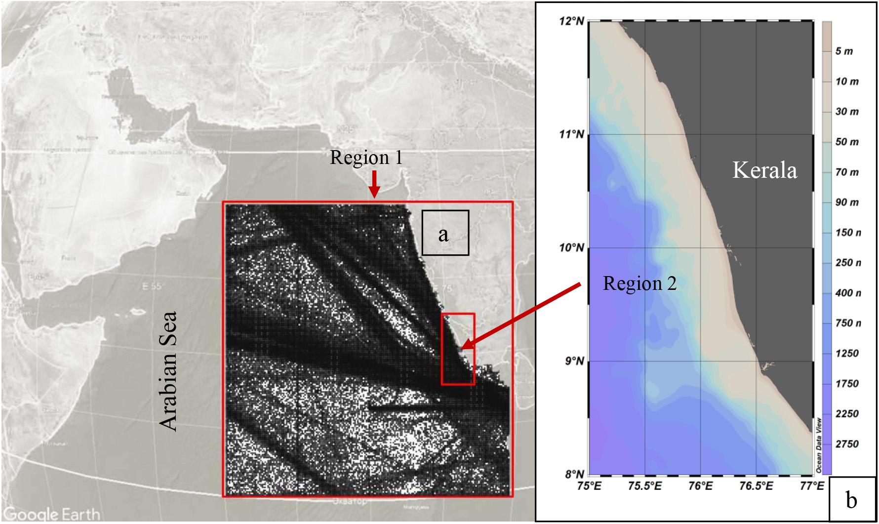
Figure 1. Study region including Kerala coast, India and coordinates (points) of VOS wave data available in the Global Wave Atlas for 1970–2018. The study regions 1 (a) and 2 (b) in the Arabian Sea are marked in squares.
Mudbanks prevail in semi-circular shape and extend up to 8–10 km offshore in water depth up to 15 m and 3–4 km alongshore. As was shown mud dominated bottom can damp the waves (Rajesh Kumar et al., 2008; Parvathy and Bhaskaran, 2019) and this effect comparable with wave attenuation due to the vegetation (Samiksha et al., 2019). Samiksha et al. (2017) studied the wave attenuation due to the MBs using measurements and modeling and found that 65–70% of waves dampened in the MBs area. Philip et al. (2013) found that the formation is associated with increased upwelling along the coast. Jacob et al. (2015) and Loveson et al. (2016) argued over the validity of subterranean conduit flow of mud/water from the Vembanad Lagoon. Shynu et al. (2017) carried out seasonal time series measurements of suspended particulate matter in the MBs region and postulated that the dissipated wave energy might have probably eroded the bottom sediment and formed the near-bed fluid mud. As was recently shown in Saprykina et al. (2020), wave dissipation leads to frequency downshifting process in wave spectra due to difference of wave attenuation coefficients at the beginning and the end of this process will lead to formation first erosive and then accumulative profile, i.e., MB. Though different hypotheses were proposed for explaining the formation of MB, none of them is conclusive due to lack of convincing scientific/field supports holistically.
When we compare earlier study of Mathew et al. (1995) with recent studies, we can show that the frequency of MB occurrence has reduced in the recent years (Noujas et al., 2013; Parvathy et al., 2015). Therefore, in the present study, we made an attempt to investigate the possible connection between the frequency of occurrence of MBs and variability in wave climate of the eastern AS.
The North Indian Ocean (NIO) comprises of two basins, namely, the AS and the BoB. The wave climatology in the NIO changes primarily due to wind reversal during two seasons—SWM and northeast monsoon (NEM). Wave characteristics in both the basins are different during the two seasons. The wave climate of eastern AS is described by many researchers (Prasada Rao and Baba, 1996; Kumar et al., 2000; Amrutha et al., 2016; Nair and Kumar, 2016; SanilKumar and Jesbin, 2016; Naseef and Kumar, 2017) based on various datasets. The wave climate of the eastern AS shows seasonal variability with maximum wave height during SWM (Sanjiv et al., 2012; Glejin et al., 2013b; Anoop et al., 2014; Kumar et al., 2014). Johnson et al. (2012) studied wave parameters at three locations in the eastern AS during SWM, and found increase in significant wave height (SWH) as we move from south to north. Shanas and SanilKumar (2014) and Glejin et al. (2013b) studied the changes in wind speed and SWH in the eastern AS by analyzing 34 years of ERA data and concluded that the average SWH in the eastern AS during pre-monsoon (February–May), SWM (June–September), and post-monsoon (October–January) are about 1.0, 2.7, and 0.7 m, respectively, with an annual average value of approximately 1.1 m. Few studies (Neetu et al., 2006; Glejin et al., 2013b; Amrutha et al., 2016) also proved that the wind waves of the eastern AS are also strongly affected by the diurnal variations of sea/land breeze activity during the non-monsoon period. Wave climate along the west coast of India (WCI) is dominated by swells during SWM and NEM and by wind seas during pre-monsoon season (Prasada Rao and Baba, 1996; Kumar et al., 2000; Aboobacker et al., 2011; Vethamony et al., 2011). In the eastern AS, SWHs are generally low during NEM and pre-monsoon, and higher during SWM (Kumar and Kumar, 2008; Vethamony et al., 2009; Aboobacker et al., 2011). Long period Southern Ocean swells are also observed in the eastern AS, except during SWM (Glejin et al., 2013a,b). Recently, Sreelakshmi and Bhaskaran (2020a,b,c) carried out detailed studies on the wind and wave climatology in the IO, using global datasets such as ERA-Interim, ERA40, and ERA5. They divided IO into different sectors based on diversified wave characteristics and discussed the trends in wind and wave climate, sector wise in the whole IO.
Stopa and Cheung (2014) studied the periodicity and patterns of global ocean wind and wave climate and revealed that wave climate of IO and Pacific Ocean depends on the El Niño/Southern Oscillation (ENSO) and Antarctic Oscillation (AAO). Anoop et al. (2016) examined the impact of IO Dipole (IOD) on the surface wind field of the AS and its impact on the wave climate during October, when the winds are weak and the IOD is the strongest. Their study concluded that the IOD impact depends on variations in the wind fields during different phases of IOD event. Decrease in SWHs was observed in the central and southwest coast of India during positive phase of IOD, whereas SWHs increase during the negative phase of IOD. They also observed that in the eastern AS, IOD impact is stronger than ENSO with more effect in the central eastern AS. A study carried out by Chowdhury and Behera (2017) made an attempt to investigate the effects of a changing wave climate on longshore sediment transport (LST) along the central WCI. They tried to link the variability in wind waves and swells with the changes in the LST over the period of time. Their study concluded that the decay in LST is directly linked to the decrease in the wave activity. As of now, there are numerous study on various aspects related to MB of Kerala, but the impact of wave variability on the occurrences of MB is still unexplored.
Therefore, in the present paper, we studied the variation of wave climate through climate indices, and explored the possible connections of these fluctuations with appearance of MBs and their evolution in different years. For the analysis of wave climate of the eastern AS, visual observations made from the voluntary ships (VOSs) were used. The temporal variability (both intra-annual and multi-decadal) in wave climate of the eastern AS is related with the main climate indices, and based on that, occurrence of MBs over the years is discussed.
Data and Methods
Wave Data
The available field wave data are not sufficient and suitable for this type of analysis to investigate the relationship between wave climate and main climate indices describing the dynamics in the Indian Ocean (IO) because of their temporal and spatial limitations. The reanalysis wave data could not be used for this analysis, due to the main disadvantage of poor reproduction of wave conditions in the nearshore and on long time scales (decadal periods) because they are based on wind reanalysis. This is determined by the errors in the reanalysis of wind data for long periods back to time and the discrepancy between the reanalysis of wind data and observations in the coastal zone. When analyzing climatic changes, this can lead to the detection of spurious trends (Bloomfield et al., 2018) or, conversely, not to detect changes on multi-decade periods (Saprykina et al., 2019). In Samiksha et al. (2017), discrepancies in the buoy and model wave heights were attributed to the possible formation of MBs (model could not accurately reproduce nearshore wave heights). Wave measurements available for this region are very rare and limited to a few months only. In this situation, visual observations are the only source of data available in the coastal zone of Kerala. Therefore, for the analysis of wave climate, visual observations made from VOSs have been used. The successful use of these data for the analysis of climate change is shown in many scientific papers (Barnett, 1983; Gulev et al., 2003). Validation of these data is available with full-scale field measurements by buoys and radars, and a good similarity is observed (Soares, 1986; Grigorieva and Badulin, 2016; Grigorieva et al., 2017). In the past, along the coast of India, Chandramohan et al. (1991) visually observed wave and current data were used to estimate LST along the north Karnataka coast. The quality of visual observation data in relation to measured and model data is discussed in detail in Soares (1986); Gulev et al. (2003), and Grigorieva et al. (2017). The discrepancies between VOS data and measurements are mainly found while comparing non-averaging observations. Otherwise, when comparing with monthly mean or annual data, the accuracy has significantly increased, and as noted in Gulev et al. (2003) for many locations, observational uncertainties are within 20% of mean values, which is acceptable for climatological studies. The accuracy also depends on the number of observations. From this point of view, the IO has very large number of wave observations, as the ship traffic is huge. In general, the accuracy for VOS data is 0.5 m for wave heights, 1 s for periods, and 10° for directions (Gulev et al., 2003; Grigorieva et al., 2017). It is very well comparable with altimetry data (0.4 m for wave heights, no wave period, 17–20° for directions) and buoys data (0.2 m for wave heights, 1 s for periods, 10° for directions) (Grigorieva and Badulin, 2016; Saprykina and Kuznetsov, 2018a).
Voluntary ship data were extracted from the Global Wave Atlas, which was created at the Shirshov Institute of Oceanology of Russian Academy of Sciences. The details of VOS data included in the Atlas, methods of preprocessing (artificial errors correction or elimination, correction of small wave heights, checking extreme wave heights and inconsistency of wave parameters, checking the accuracy of wind sea and swell separation, applying the steepness and wave age control using combined criteria, etc.), and validation are described in Gulev et al. (2003); Freeman et al. (2017), and Grigorieva et al. (2017). Quality checked data of Wave Atlas include about 30% of all available VOS data. In the observation scheme of VOS, wave parameters (SWH and mean wave period) of wind waves and swells are recorded separately, first on the basis of expert visual assessments of observators (seafarers and ocean scientists), and second, in accordance with the unified methodology adopted for such observations in recent decades. Waves propagating in the absence of wind, long waves with a direction different from wind and any other genesis of which cannot be associated with the effect of wind, can be classified as swell waves. Most of the observations in the Wave Atlas additionally provide information such as wind speed and direction, data, time, coordinate (longitude, latitude), wave period, etc. For the IO, such records are available since 1888; however, the most complete data (in particular, wave height and period of wind waves and swell, wind speed, direction of propagation, and coordinates) and verified database are available from 1970 only. Thus, from the IO dataset, we have extracted data for the period 1970–2018 in the domain extending from 0° to 20°N and 60° to 85°E (Region 1) (Figure 1). A separate sub-region including Alleppy coastal zone was also extracted along the coast of Kerala extending between 8°–12°N and 75°–77°E (Region 2).
Figure 2 shows the number of observations extracted from January 1970 to December 2018 by month, dependences of available wave height on the number of observations, and wave parameters (height and period) for a site near the coast (region 2) and region 1, without region 2. Figure 2 clearly shows that the number of observations near the coast of Kerala is significantly less, but at a qualitative level, the wave parameters are approximately the same. The heights of wind waves and swells near the shore (region 2) are slightly lower. Near the coast, waves with a period of the order of 1 s were recorded, while in region 1, such waves were practically not observed (Figures 2E,F). For both swells and wind waves in the selected regions of IO, there is slightly dependence especially of large wave height on the number of observations (Figures 2B,D). This is quite understandable, since high waves are less common than low ones, and the more observations, the more likely to register higher waves. When comparing the wave heights in the two regions, no significant qualitative difference, for example, possibly caused by the presence of MBs, is observed. The dependence of the wave height on the period has the same character (Figures 2E,F).
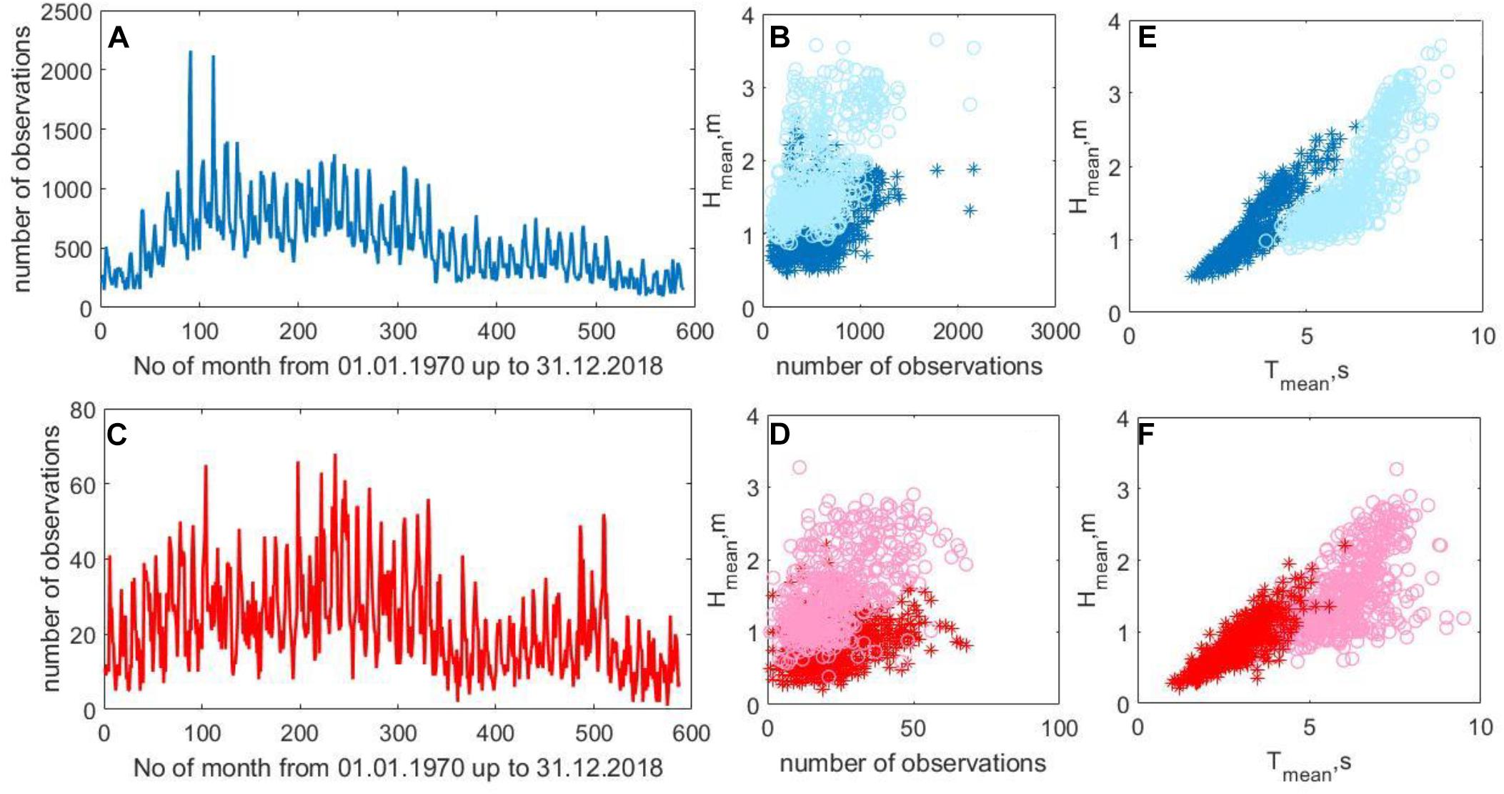
Figure 2. Number of observations by months from January 1970 to December 2018 (A,C), dependence of wave height on the number of observations (B,D), and dependence of wave height on wave period (E,F) for region 1 (excluding region 2, blue and light blue colors) and region 2 (red and pink colors), respectively. Circles represent swells, and stars represent wind waves.
To verify the data of VOS observations, we additionally compared the VOS data with available waverider buoy data measured off Kerala coast (near MB region, region 2). Two waverider buoys were installed in Alleppy coastal zone at 15 m water depth (May21 to July 31, 2014) and 7 m water depth (June 26 to July 31, 2014) at the distances 10 and 6 km from the shore, consequently. More details about the field measurements are given in Samiksha et al. (2017). The comparison of SWHs between available VOS observations nearshore and buoy measurements is shown in Figure 3.
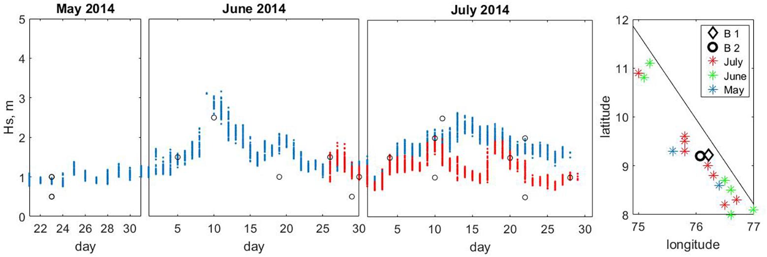
Figure 3. Comparison of wave heights between VOS data (black circles) in region 2 and buoy measurements at 15 m (blue point) and 7 m (red points) water depths and coordinates of observations and buoys. The line approximately separates land and sea.
Figure 3 shows the qualitative coincidence change in SWHs. The observed differences in the heights are explained by differences in the averaging methods. The buoy data are obtained as a result of averaging the 20-min time series, and the data of VOS observations are actually given as non-averaged parameters of the observed individual waves. Inconsistencies can also be due to wave shoaling and dissipation in nearshore zone.
Climatic Indices
The following main climate indices, which traditionally reflect the influence of El Niño phenomenon in the AS in which the monsoon intensity is associated with the dynamics of the IO were considered in the present study: (i) IOD, (ii) Southern Oscillation Index (SOI), (iii) AAO, (iv) ENSO, (v) El Niño phenomenon index for the site 5N-5S and 170W-120W (NINO3.4), (vi) Pacific Decadal Oscillation (PDO), and (vii) Atlantic Multi-decadal Oscillation (AMO). The time series of these indices and their description are available on websites of the offices of the US National Oceanic-Atmospheric Agency https://www.cpc.ncep.noaa.gov and https://www.esrl.noaa.gov. The time series of NINO3.4, ENSO, IOD, AMO, and SOI from 1970 to 2018, PDO from 1970 to 2017, and AAO from 1979 to 2018 were analyzed.
Methods of Analysis
For analysis, the wave heights were monthly averaged. As the time series of monthly averaged VOS data are short (49 years or 588 months), in order to obtain periodicity, especially, the decadal and multi-decadal scales, instead of using the classical spectral analysis based on FFT and DFT methods, we have used the Yule-Walker parametric method and the method of continuous wavelet transform with the Morlet wavelet function (Torrence and Compo, 1998; Saprykina and Kuznetsov, 2018a,b).
The Yule-Walker parametric method of spectral analysis is based on applying an autoregression model on the data series, in which the variable to be studied will linearly depend on its own previous values and on some stochastic term (Stoica and Moses, 2005). For sinusoidal time series, Yule-Walker method allows us to determine the period even if the length of the series is about half of the period, i.e., for our study, it is possible to detect period about 98 years. For long time series or for short-time periodicity, the results of classical spectral analysis (FFT and DFT methods) and Yule-Walker method will be the same (Stoica and Moses, 2005). So Yule-Walker parametric method of spectral analysis will allow detecting at the same time both multi-decadal (for which length of data is very short) and monthly periods (for which length of data is enough).
Wavelet transform is a kind of scanning of time series by frequencies. Like Yule-Walker method, it allows us to determine the periodicity of processes in short series of half the specified period. In addition, wavelet analysis represents the fluctuation of the spectrum in time, in contrast to the spectral analysis, which averages the spectrum over time. This allows us to assess the structure of the process as a whole and analyze its stationarity/non-stationarity. As shown in Saprykina and Kuznetsov (2018a,b), fluctuations of climatic indices (for example, AMO and PDO) are non-stationary in time and can be non-linear due to modulation of high frequencies by low frequencies. In this case, the use of classical correlation analysis applied to linear stationary processes is impossible. Therefore, to obtain the correlations, we have used the recently developed method of wavelet correlations. Wavelet-correlations method is the construction of a correlation function between the wavelet transforms of two signals for the same wavelet-frequency bands. It is analog to the classical correlation analysis, when original signals are initially filtered on a set of narrow-banded signals of characteristic frequency bands, and then the correlations between these narrow-banded signals are analyzed. If the number of such narrow-banded signals is sufficiently large, then each narrow-band signal can be considered as a quasi-stationary signal, and makes it possible to analyze the correlations between two non-stationary processes.
Results and Discussion
Homogeneity of Arabian Sea Wave Climate
The changes in the monthly averaged heights (MAH) of the wind waves and swells for regions 2 and 1 are shown in Figures 4B,E. The MAH of swells do not have a linear trend; however, the heights of wind waves show a slight increase in the last one decade. MAH of waves have periodic fluctuations. Maximum fluctuations occur during the year and the maximum number of SWH in a year appears in the summer months (June–August) for both the regions (Figures 4A,D). However, in some years, in region 2 near the coast, the highest swells were observed in September (Figures 4A,D). In general, the long-term average annual cycle of changes in MAH of waves is similar for both the regions (Figures 4C,F), except that the maximum MAH of wind waves in the coastal region are observed in June and in the offshore (region1) in July. This may serve as an indirect sign that peak of the MBs formation is observed in the coastal region in July (Samiksha et al., 2017) and attenuate the waves, compared to the rest of the eastern AS.
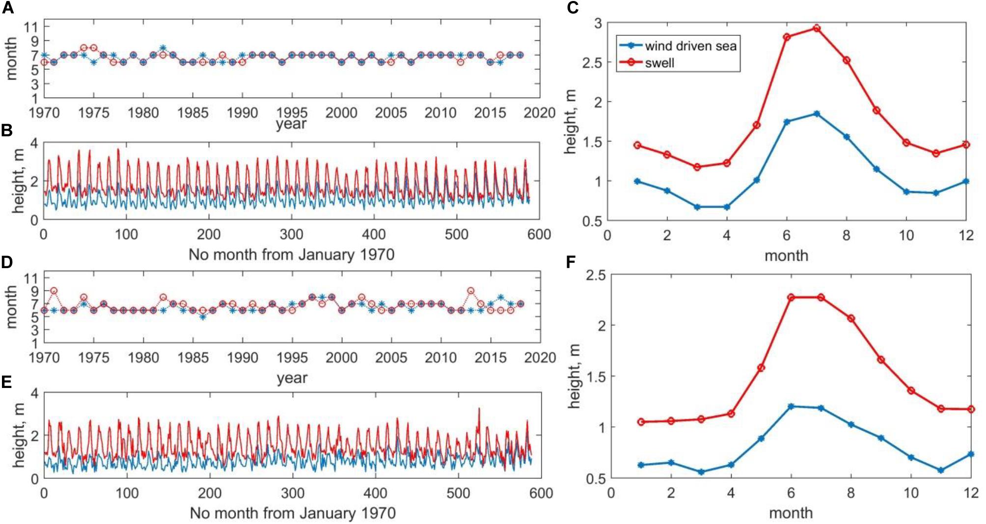
Figure 4. The month in which the highest average monthly wave height is observed, the change in the average monthly height of wind waves (blue) and swells (red) and the annual change in the heights of wind waves and swell averaged from 1970 to 2018 for region 1 excluding the region 2 (A–C) and region 2 (D–F).
Figure 5 shows that qualitatively the fluctuations and trends in monthly averaged wave heights are the same for both the regions. The relationship between them is linear with a coefficient of 1.1, the deviation from 1 is due to the fact that the data of region 2 contain more nearshore data and, in general, their height is 0.2 m less. Taking into account the analysis of the heights of individual waves of the two regions, made above, we can assume that the data of monthly averaged wave heights in the two regions of eastern AS are homogeneous (Figures 2, 5). Therefore, it can be expected that changes in wave climate will occur in the same manner for both the coastal and the offshore regions. Hence, in order to analyze the wave climate variability, we have merged the data of both the regions to have more data for reliable analysis. The wave data homogeneity of the two regions also indicate that the AS as a whole can influence the dynamics/formation of MBs.
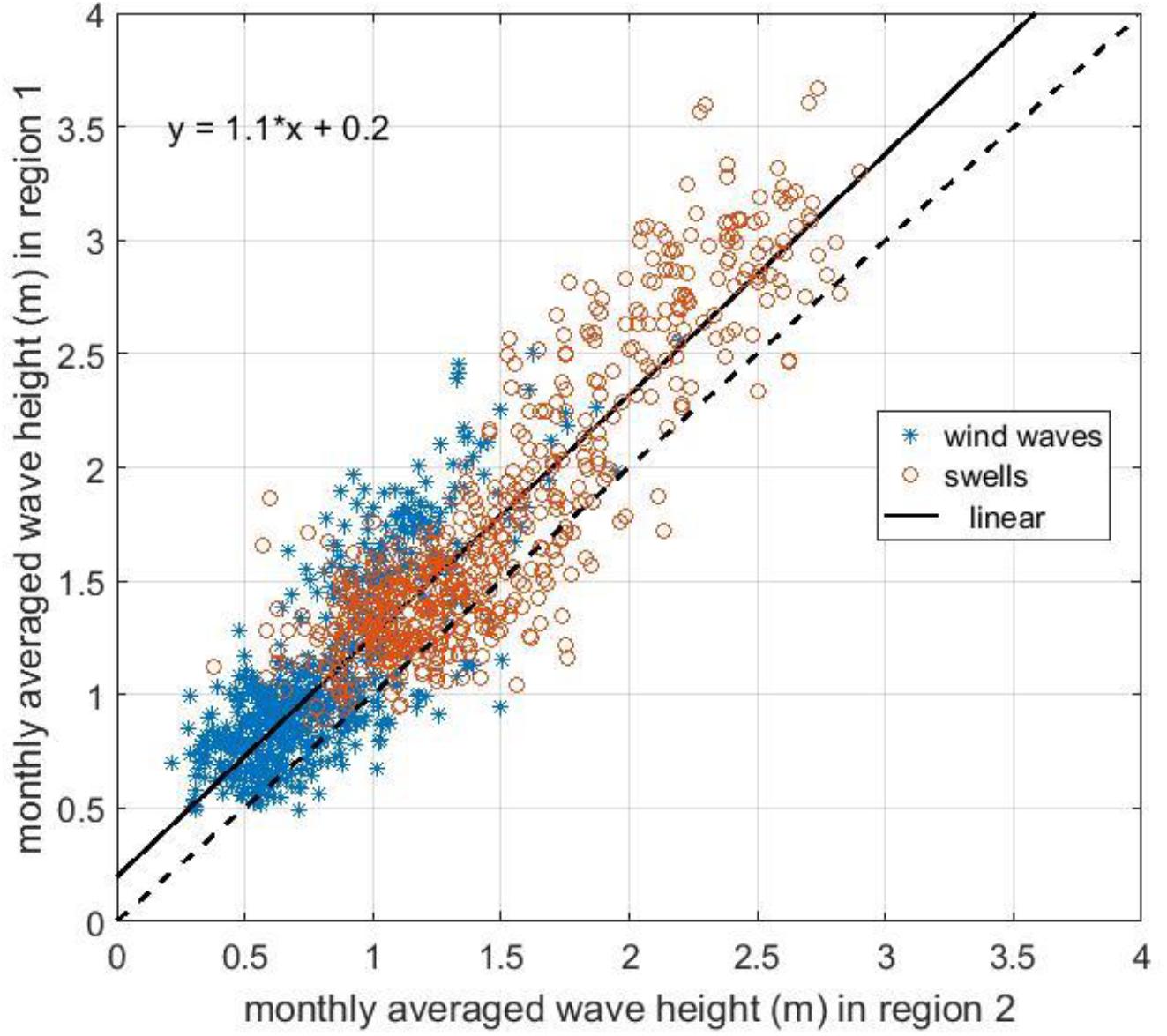
Figure 5. Monthly averaged wave height in region 2 versus region 1 (excluding region 2) for wind waves (blue) and swells (red).
Variability of Arabian Sea Wave Climate
Figure 6 and Supplementary Figure 1 present the results of spectral parametric analysis performed by the Yule-Walker method and a wavelet analysis for the changes in the MAH of wind waves and swells for region 1. For analysis, mean value and linear trend were removed from the time series of monthly averaged wave heights. It is clearly seen that the characteristic periods observed at small time scales are the annual and semi-annual variability of wave heights (both swells and wind waves), associated with SWM in the summer period (June–July) (Figure 4). The characteristic peaks of this variability are present both on the spectra and on the wavelet diagrams. According to wavelet analysis, fluctuations in this time range for the period 1970–2018 are almost stationary, and have no visible time trends (Figures 4, 6 and Supplementary Figure 1).
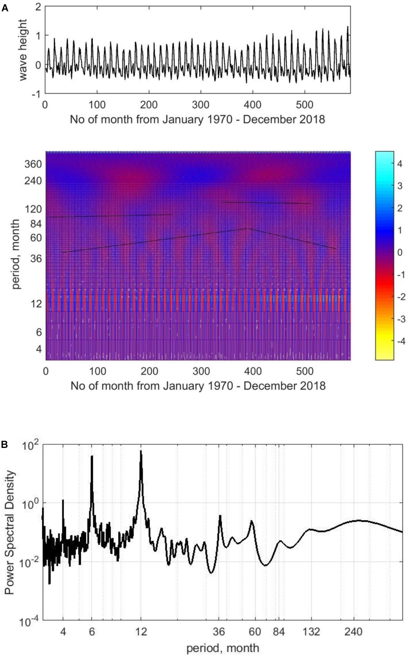
Figure 6. Change in monthly averaged heights of wind waves. Wavelet transform (A) and power spectral density Yule-walker method (B) (for wavelet analysis, mean value and linear trend were excluded from height series). The lines show the available trends in coefficient fluctuations.
As for the decadal and multi-decadal oscillations of average monthly wave heights are concerned, it is clearly seen on the wavelet diagrams (Figure 6 and Supplementary Figure 1) that the periods of these oscillations are non-stationary, and there are linear trends in their periods, both for wind waves and for swells (for example, in the range of periods from 40 to 200 months). The non-stationary nature of the process of changing the monthly averaged wave heights at these time scales does not allow the use of spectral analysis to clearly distinguish periods in this range, especially for wind waves (Figure 6 and Supplementary Figure 1, spectra), although this periodicity is clearly visible on wavelet diagrams. In general, based on the results of spectral and wavelet analysis, it can be stated that changes in average monthly heights of wind waves and swell waves have the same variability on periods of 6 months, 1 year, 3 years, 4–5 years, and 7–8 years, and similar periodicity on longer and multi-decadal scales in range about 10–16 and 20–40 years.
Variability of Climate Indices
The results of wavelet analysis show that the changes in the selected indices are also non-stationary. To save this article space, we have discussed only two of them—IOD and NINO3.4. For example, changes in IOD index have a pronounced trend on the scales of variability from 50 to 100 months and from 350 to 200 months (Figure 7A). Changes in the NINO3.4 index have a visible trend in the period range, 100–200 months (Figure 7B). At the same time, the variability of both indices is stationary in the range of 6–12 months. The unsteady nature of PDO and AMO changes has been discussed in detail in Saprykina and Kuznetsov (2018a, b). Thus, the wavelet analysis made it possible to explain the non-stationarity of changes in all indices in a given time range.
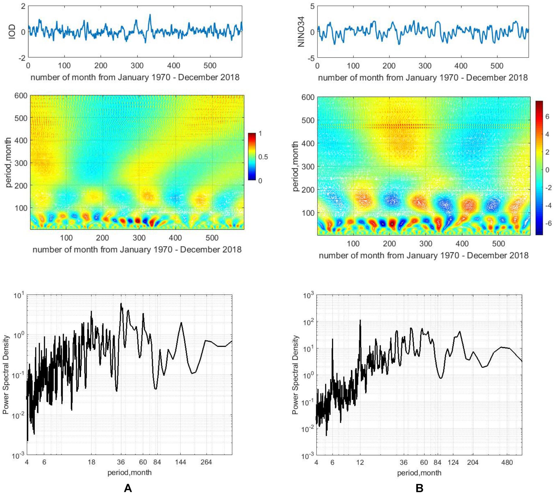
Figure 7. Fluctuations of IOD (A) and NINO3.4 (B) indices and their wavelet transform (top), power spectral density Yule-walker method (bottom). For wavelet analysis, mean value and linear trend were excluded from indices.
Analysis of Connection Variability of Monthly Averaged Wave Heights With Climate Indices
As expected the classical correlation analysis showed rather low correlations with the select climate indices (correlation coefficients are less than 0.2), except for correlation with NINO3.4 index—correlation coefficient is 0.39. Such low connections can be explained by the non-stationary changes in both wave heights and indices. To obtain correlations between non-stationary processes, the wavelet correlation method has been used in the present study. The wavelet correlation coefficients at zero time lag for MAH of wind waves and swell waves are shown in Figure 8. The corresponding wavelet cross correlation diagrams, for some indices versus time lags, are shown in Supplementary Figure 2.
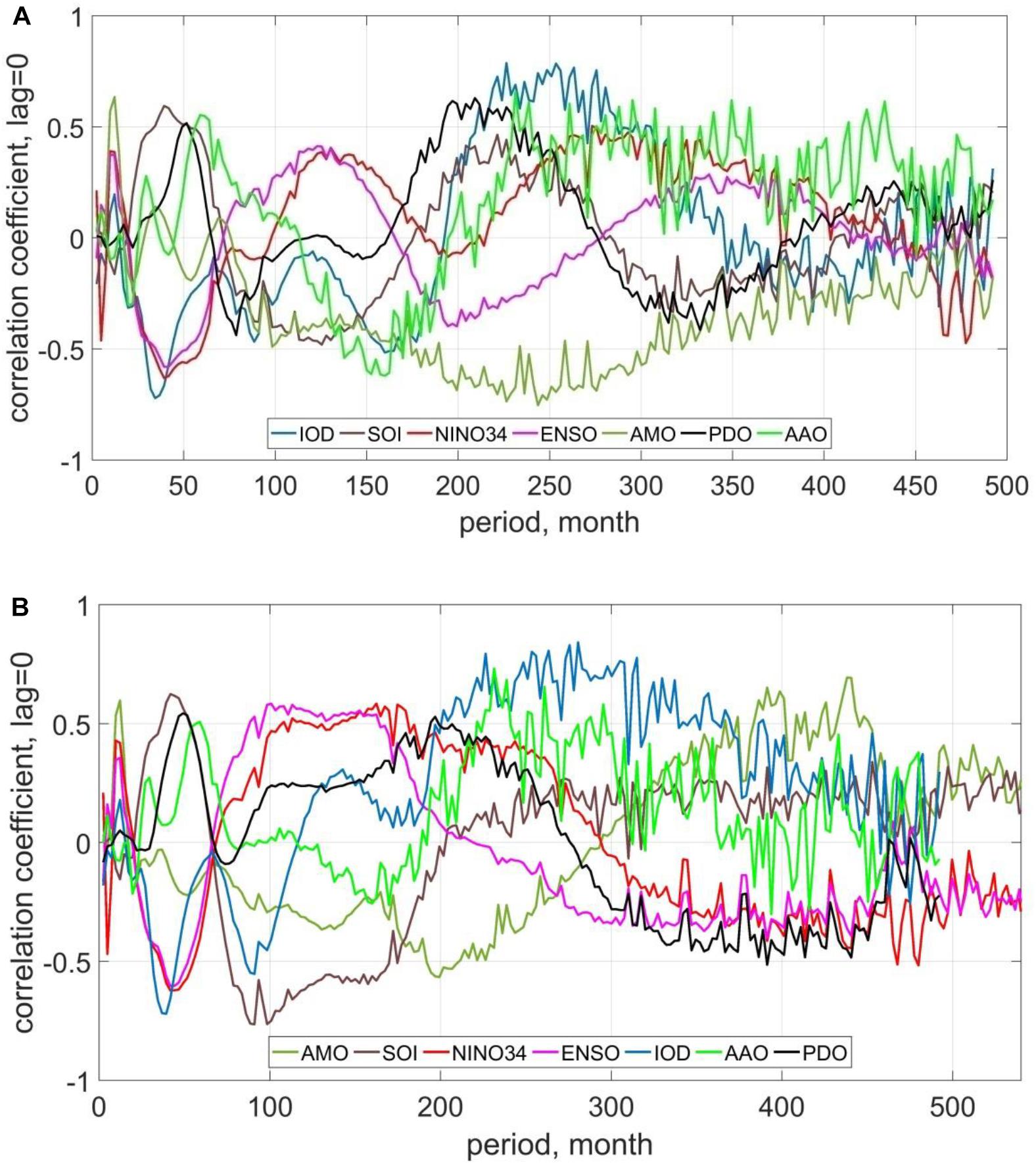
Figure 8. Wavelet correlation coefficients between changes in climate indices and averaged monthly height of wind waves (A) and swell waves (B) at zero time lag.
A zero time lag means that two processes occur simultaneously. It can be seen that for periods less than a decade, changes in the heights of wind waves and swell waves are associated with changes in the same climate indices. Some differences are observed in periods more than 10 years. Supplementary Table 1 shows the characteristic periods of variability of the monthly averaged wave heights and swells and their correlation (correlation coefficient > 0.4) with the select climate indices.
The correlations between some indices will be significantly higher if we take into account the time lag between climate processes and the change in wave heights (Supplementary Figure 2). For example, the positive phase of the annual and semi-annual changes in the NINO3.4 index leads to an increase in wave heights with a lag of 2 months (correlation coefficient is 0.80 for both the periods). There is 1-year lag between the positive phase of NINO3.4 oscillations with a period of about 10 years and the averaged monthly wave heights (correlation coefficients are 0.50 and 0.80, for wind waves and swells, respectively) (Supplementary Figures 2c,d). The lag between positive phase of the ENSO change during the year and 6 months and increase in wave height occurs with a lag of 1 month with correlation coefficients of 0.60 and 0.68 for wind waves and swells in both periods, respectively. A negative phase of SOI oscillation with a period of about 10 years will lead to an increase in the height of wind waves and swell waves with a lag of 1 year (correlation coefficients are negative: −0.60 and −0.75, respectively), and a positive phase of oscillation with a period of 20 years will have a lag of 2 years (correlation coefficient is 0.70) (Supplementary Figures 2a,b). The positive phase of ENSO index leads to an increase in wave heights for a period of 10–13 years with a lag of 6 months to 1 year, both for wind waves and for swell waves (correlation coefficients are 0.55 and 0.70, respectively). Also, a positive phase of ENSO oscillation with a period of 16 years correlates with an increase in the height of wind waves with a lag of 2 years (correlation coefficient is 0.50). The negative phase of AMO with 7–8 years period of oscillation will lead to an increase in the height of wind waves after 1 year (correlation coefficient is −0.65), and the positive phase of oscillation with a period of 16 years will also increase the height of swells after 1 year (correlation coefficient is 0.80) (Supplementary Figures 2e,f).
The negative phase of fluctuations in the PDO index with a period of 16 years leads to an increase in the swell height with a lag of 2 years (correlation coefficient is −0.65) (Supplementary Figures 2g,i). Also, in the diagrams of wavelet correlations (Figure 6 and Supplementary Figure 2), one can notice a rather high correlation between changes in wave heights and fluctuations of climate indices occurring with a time lag, which was not detected at zero time lag. So, for a change in the MAH of swells, a variability of 13 years period associated with fluctuations in the IOD index exists, like the monthly averaged wind waves, but it is lagged by about 2 years (correlation coefficient is −0.65).
For the SOI index, there is a relationship between a period of change of 20 years and fluctuations in the average monthly swell height as well as for wind waves, lagged by 2 years (correlation coefficient is 0.55). For the NINO3.4 index, there is a high correlation between the increase in the height of wind waves and its positive phase for a period of 16 years with a lag of 2–3 years (correlation coefficient is 0.65).
An increase in the MAH of wind waves with a period of 3 years can be associated with a positive phase of oscillations of the AMO index over the same period (correlation coefficient is 0.60) and occurs 6 months later. There is also a relationship between the negative phase of fluctuations in the AMO index with a period of 8 years (correlation coefficient is −0.50) and the increase in the height of swells that occurs after a year.
The annual fluctuations in the heights of both wind waves and swells are closely connected to fluctuations in the PDO index, lagged by 3 months. A correlation between the negative phase of AAO fluctuations with periods of 12–13 years and an increase in the height of swells (correlation coefficient is −0.80) with a lag of 1 year has been identified (Supplementary Figures 2j,k). It should be especially noted that the averaged monthly height of wind waves varies in phase with fluctuations in the IOD index over the periods 3, 7, 13, and 20 years.
Thus, as a result of the analysis, the following periods of fluctuations in the MAH of wind waves and swells were identified: 0.5 year (associated with NINO3.4 and ENSO), 1.0 year (due to a change in NINO3.4, ENSO, AMO, and PDO), 3.0–3.5 years (associated with a change in NINO3.4, ENSO, SOI, and IOD), 4.0–5.0 years (associated with a change in PDO and AAO), 7.0–8.0 years (associated with a change in IOD and AMO), 10.0 years (associated with a change in SOI, NINO3.4, and ENSO), 12.0–13.0 years (associated with a change in IOD and AAO), 16.0 years (associated with a change in NINO3.4 and PDO), 20.0 years (associated with a change in SOI, NINO3.4, and AAO) and 30.0 years (associated with a change in PDO and AAO). For all indices except PDO, there are high correlations on periods about 40 years. Note that on all time scales, the most significant connection between the wave climate and the El Niño phenomenon changes in which are directly or indirectly taken into account in the indices NINO3.4, ENSO, SOI, and PDO.
Possible Connections of Arabian Sea Wave Climate Fluctuations and Occurrence of Mudbanks
As discussed in Section “Introduction,” there have been many studies dealing with various aspects of appearance and disappearance of MBs at various locations along the Kerala coast. Numerous studies confirm the fact that high waves during the monsoon period initiate the appearance of MBs. This gives us a reason to speculate and form a hypothesis about how the identified periods of fluctuations in wave heights could influence the evolution of MBs and how this is confirmed by the available observations.
In Mathew et al. (1995), measured SWH and time of existence of MB off Alleppy in summer monsoon of 1986–1989 are shown in the same figure. It can be seen from this figure that the time of appearance and duration of existence of MB depend on the maximum wave heights in the summer monsoon cycle. So, if the maximum wave heights were in May-early June during 1986–1989, MBs were observed from mid-June to mid-July (in 1989). If the height of maximum waves was observed in mid-June, MB appeared from mid-July to end of August (in 1986). In 1988, the highest waves were observed in June and July, which corresponded to the existence of MB from mid-June to early August. This indicates that the time of appearance of MB and their “lifetime” are associated with distribution of maximal SWH in the monsoon cycle. Despite the fact that the maximum MAH of wind waves and swells in the monsoon cycle during 1979–2018 have been observed in June, it is clearly seen that there are deviations from this average cycle, when the largest waves are observed in other months (Figure 4). In Figure 9, changes in the monthly averaged SWH during summer monsoon years in which observations of times of appearance and times of existence of MBs in the Kerala region are available are presented in Philip et al. (2013).
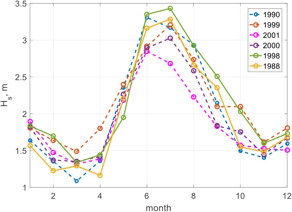
Figure 9. The monthly averaged SWHs in the Arabian Sea for select years according to VOS data.
SWH is calculated using the following formula:
where Hwind = SWH of wind waves and Hswell = SWH of swells.
If we refer to Figure 9, we find that in 1990 and 2001, MBs appeared off Kerala in June, which corresponds to the time (month) of maximum monthly averaged SWH. In 1999, they were observed during May–September, which corresponds to the time of higher waves already set in May and the peak of monthly averaged SWH in July. In 2000, MB appeared in August, and maximum monthly averaged SWH was observed in July. In 1988 and 1998 (10 years period), MBs were observed from June to August, and, as can be seen in Figure 9, this corresponds to approximately the same summer monsoon cycle of monthly averaged SWH, with maximum heights in June and July. According to the results of wave climate analysis carried out in the previous section, the possible 10-year periodicity of such a cycle could be related to the influence of climate indices SOI, NINO3.4, and ENSO (Supplementary Table 1).
Because the appearance of MBs depends on the heights of the waves and, as the analysis of Figure 9 shows, the wave height threshold for their formation is 2 m. As shown in Saprykina et al. (2020), the mechanism of MBs formation due to the wave transformation depends on the rate of dissipation of their energy above the bottom profile. In this case, it is important that must be two characteristic regions: first with a strong dissipation of the wave energy and then with a weak one, which will lead to the formation of an erosive (weighing of particles) and then an accumulative bottom profile due to their transfer, i.e., the formation of an MB. If the wave height is too high, then the length of the erosional area will significantly prevail, the particles will be in a suspended state, and the MBs will not have time to form. Therefore, MBs sometimes form not in the months when the highest waves were observed, but in the following months, when the wave height is lower, for example, in 1988, 1998, 1999, and 2000 years. In general, knowledge of the patterns of annual and long-term changes in wave heights in the monsoon cycle can also make it possible to predict the time of the appearance of MBs on different parts of the Kerala coastline due to the features of wave transformation over the bottom topography of each area.
Let us discuss how does the maximal of the monthly averaged SWH in summer monsoon cycle changes during 1970–2018. Figure 10A shows a series of these maximal (mean value is removed) and its wavelet transform. Figure 10B shows the corresponding wavelet correlation coefficients with climate indices SOI, NINO3.4, ENSO, and IOD at zero time lag. Periods of the order of 7, 10–12, 18–20, and about 40 years associated with the fluctuations of these climate indices are clearly visible. It is confirmed by high values of modulus of the wavelet correlation coefficients (Figure 10B).
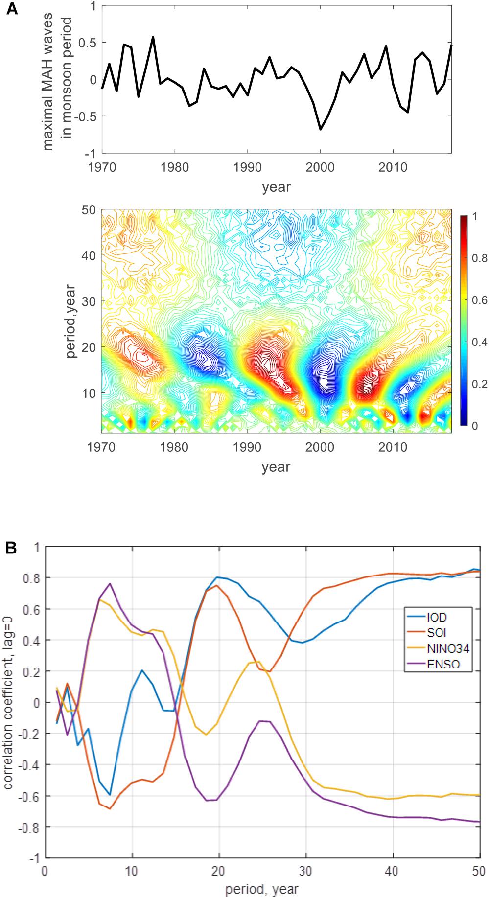
Figure 10. Maximum of monthly averaged SWH in summer monsoon cycle and its wavelet transform (A) and wavelet correlation coefficients with climate indices at zero time lag (B). For wavelet analysis, mean value and linear trend were excluded from indices.
Webster et al. (1999) noted that El Niño events have indirect influence on IO and can force it to coincide with periods of its internal dynamics. Although IOD is considered as the main climate index of IO dynamics, as can be seen from Figure 10B, the combined mutual influence of SOI, NINO3.4, and ENSO indices in addition to the influence of IOD determines the main important periods of variability of the maximum monthly averaged SWH during the monsoon period: 7, 18–20, and about 40 years.
Parvathy et al. (2015) have listed out the occurrences of MBs off southwest coast of India by taking into account all the reported data in the past and also discussed the significance of the recent and past MB in coastal dynamics. They reported that the best known MB of the southwest coast of India is Alleppy. Earlier reported areas of MB formation are the Munambam–Chettuwa sector at Chettuwa, Vadanappally, Nattika, Thalikulam, and Kaipamangalam (Mathew et al., 1995). But, presently these locations do not show any occurrences of MBs, and as reported by Noujas et al. (2013) during monsoons (2009–12), the MB occurrences were observed at Kara to Kaipamangalam sector. As reported in Noujas et al. (2013), based on the literature survey and interaction with the local people in the studied area, the location of occurrence of MBs moved southward from Chettuwa to Thalikkulam to Nattika to Edamuttam to Kaipamangalam to Bhajanamdom successively during the last 40 years, and it remained stable in the same sector for 5–10 years. From 2013 onward, the occurrences of MB were reported in the Thykal and Punnapra region, Alleppy. About 10–12 years back, MBs which were seen confined to Purakkad region have moved south toward Punnapra region and since then it is forming at Punnapra region repeatedly (Parvathy et al., 2015).
The movement of MBs southward could be connected to the identified about 40 year period of El Niño events—for example, its influence on Monsoon Current in the IO (Webster et al., 1999). Suppose such possible influence is applied on West India Coastal Current (WICC), it could transport huge volume of water and suspended sediments from the coastal northern AS into the southeastern AS so that MB movement can be associated with simultaneous long-term fluctuations (about 40 years) of IOD, SOI, and El Niño. Unfortunately, the absence of detailed systematic long-term observations at least in a few locations in the study region does not allow us to obtain unambiguous clear connections between fluctuations of the wave climate and MBs occurrence. However, the above reasoning about the relationship between wave climate fluctuations is in a good agreement with the visual long-term observations of MBs evolution on the Kerala coast available in the literature. Thus, we hypothesize possible periods of movement of MB with the main climate indices, which further requires verification of other data.
Conclusion
The analysis of wave data of VOS observations for the period 1970–2018 showed that the annual periodicity of changes in wave climate in the eastern AS, both in the coastal region and in the offshore is associated with the summer monsoon.
It has been found that the El Niño phenomenon plays a major role in the variability of wave climate of the eastern AS in all time scales, and its influence is directly or indirectly taken into account while calculating climate indices such as NINO3.4, ENSO, SOI, and PDO. The influence of El Niño is manifested with a delay of several months (3–6) on annual time scales and about 1–2 years on a decadal to multi-decadal time scales. To analyze the relationship between the change in the wave climate of this region and the El Niño fluctuation, the NINO3.4 index is recommended since it shows the maximum correlation links on all time scales of the variability.
The strong variability of the wave climate at short time scales has been identified: 0.5 year, 1 year, 3–3.5 years (with a time lag of about 6 months), 4–5 years and 7–8 years (with a time lag of about 1 year). Decadal periods of change correspond to 10, 12–13, and 16 (with time lag of about 1 year) years.
The multi-decadal fluctuations occur with a period of 20 years (correlate with IOD and AAO indices), 30 years (correlate with AAO and PDO indices), and about 40 years (correlate with IOD, ENSO, NINO3.4, and SOI).
It is shown that intra-annual fluctuations in appearance and duration of existence of MBs depend on the distribution of highest monthly averaged SWHs in the summer monsoon cycle. The monthly averaged SWH threshold for their formation is 2 m. Through annual fluctuations of highest waves in monsoon cycle, a possible relationship between the wave climate variability of the AS and the formation of MBs can be shown for the periods 7, 10–12, 18–20, and about 40 years. It correlates with fluctuation of IOD, ENSO, NINO3.4, and SOI climate indices.
Data Availability Statement
The original contributions presented in the study are included in the article/Supplementary Material, further inquiries can be directed to the corresponding author/s.
Author Contributions
YS: main idea, writing the main content of the manuscript, and data analysis. SS: writing the manuscript and archival data collection. SK: data analysis. All authors agreed to be accountable for the content of the manuscript.
Funding
This work was partly supported by RFBR Project No. 20-55-46005.
Conflict of Interest
The authors declare that the research was conducted in the absence of any commercial or financial relationships that could be construed as a potential conflict of interest.
Acknowledgments
This study was performed in the frame of the state assignment theme no. 0128-2021-0004. SS thanks Director, CSIR-National Institute of Oceanography, Goa for his support in the work. The NIO contribution number is 6708.
Supplementary Material
The Supplementary Material for this article can be found online at: https://www.frontiersin.org/articles/10.3389/fmars.2021.671379/full#supplementary-material
References
Aboobacker, V. M., Rashmi, R., Vethamony, P., and Menon, H. B. (2011). On the dominance of pre-existing swells over wind seas along the west coast of India. Cont. Shelf Res. 31, 1701–1712. doi: 10.1016/j.csr.2011.07.010
Amrutha, M. M., Kumar, V. S., Sandhya, K. G., Nair, T. B., and Rathod, J. L. (2016). Wave hindcast studies using SWAN nested in WAVEWATCH III-comparison with measured nearshore buoy data off Karwar, eastern Arabian Sea. Ocean Eng. 119, 114–124.
Anoop, T. R., Kumar, V. S., and Shanas, P. R. (2014). Spatial and temporal variation of surface waves in shallow waters along the eastern Arabian Sea. Ocean Eng. 81, 150–157. doi: 10.1016/j.oceaneng.2014.02.010
Anoop, T. R., SanilKumar, V., Shanas, P. R., Glejin, J., and Amrutha, M. M. (2016). indian ocean dipole modulated wave climate of eastern Arabian Sea. Ocean Sci. Discuss. 12, 2473–2496.
Badesab, F., Gaikwad, V., Gireeshkumar, T. R., Naikgaonkar, O., Deenadayalan, K., Samiksha, S. V., et al. (2018). Magnetic tracing of sediment dynamics of mudbanks off southwest coast of India. Environ. Earth Sci. 77:625. doi: 10.1007/s12665-018-7807-6
Balachandran, K. K. (2004). Does subterranean flow initiate mud banks off the southwest coast of India? Estuar. Coast. Shelf Sci. 59, 589–598. doi: 10.1016/j.ecss.2003.11.004
Barnett, T. P. (1983). Interaction of the monsoon and pacific trade wind system at interannual time scales part I: the equatorial zone. Mon. Weather Rev. 111, 756–773. doi: 10.1175/1520-0493(1983)111<0756:iotmap>2.0.co;2
Bloomfield, H. C., Shaffrey, L. C., Hodges, K. I., and Vidale, P. L. (2018). A critical assessment of the long-term changes in the wintertime surface Arctic Oscillation and Northern Hemisphere storminess in the ERA20C reanalysis. Environmental Res. Lett. 13:094904. doi: 10.1088/1748-9326/aad5c5
Chandramohan, P., Kumar, V. S., and Nayak, B. U. (1991). Wave statistics around the Indian coast based on ship observed data. Indian J. Mar. Sci. 20, 87–92.
Chowdhury, P., and Behera, M. R. (2017). Effect of long-term wave climate variability on longshore sediment transport along regional coastlines. Prog. Oceanogr. 156, 145–153. doi: 10.1016/j.pocean.2017.06.001
Damodaran, R., and Kurian, V. C. (1972). Studies on the Benthose of the Mud Bank Regions of the Kerala Coast. Kochi: Cochin University of Science and Technology.
Faas, R. W. (1995). Mudbanks of the southwest coast of India III: role of non-Newtonian flow properties in the generation and maintenance of mudbanks. J. Coast. Res. 11, 911–917.
Freeman, E., Woodruff, S. D., Worley, S. J., Lubker, S. J., Kent, E. C., Angel, W. E., et al. (2017). ICOADS Release 3.0: a major update to the historical marine climate record. Int. J. Climatol. 37, 2211–2232. doi: 10.1002/joc.4775
Glejin, J., Kumar, V. S., and Nair, T. B. (2013a). Monsoon and cyclone induced wave climate over the near shore waters off Puduchery, south western Bay of Bengal. Ocean Eng. 72, 277–286. doi: 10.1016/j.oceaneng.2013.07.013
Glejin, J., Sanil Kumar, V., Nair, B., and Singh, J. (2013b). Influence of winds on temporally varying short and long period gravity waves in the near shore regions of the eastern Arabian Sea. Ocean Sci. 9, 343–353. doi: 10.5194/os-9-343-2013
Gopinathan, C. K., and Qasim, S. Z. (1974). Mud banks of Kerala-their formation and characteristics. Indian J. Mar. Sci. 3, 105–114.
Grigorieva, V. G., and Badulin, S. I. (2016). Wind wave characteristics based on visual observations and satellite altimetry. Oceanology 56, 19–24. doi: 10.1134/S0001437016010045
Grigorieva, V. G., Gulev, S. K., and Gavrikov, A. V. (2017). Global historical archive of wind waves based on voluntary observing ship data. Oceanology 57, 229–231. doi: 10.1134/S0001437017020060
Gulev, S. K., Grigorieva, V., Sterl, A., and Woolf, D. (2003). Assessment of the reliability of wave observations from voluntary observing ships: Insights from the validation of a global wind wave climatology based on voluntary observing ship data. J. Geophys. Res. Oceans 108:3236.
Jacob, N., Ansari, M. A., and Revichandran, C. (2015). Environmental isotopes to test hypotheses for fluid mud (mud bank) generation mechanisms along the southwest coast of India. Estuar Coast. Shelf Sci. 164, 115–123. doi: 10.1016/j.ecss.2015.07.018
Jacob, P. G., and Qasim, S. Z. (1974). Mud of a mud bank in Kerala, south-west coast of India. Indian J. Mar. Sci. 3, 115–119.
Jiang, F., and Mehta, A. J. (1996). Mud banks of the Southwest Coast of India. V: wave attenuation. J. Coast. Res. 12, 890–897.
Johnson, G., Kumar, V. S., Chempalayil, S. P., Singh, J., Pednekar, P., Kumar, K. A., et al. (2012). Variations in swells along eastern arabian sea during the summer monsoon. Open J. Mar. Sci. 02, 43–50. doi: 10.4236/ojms.2012.22006
Kumar, V. S., and Kumar, K. A. (2008). Spectral characteristics of high shallow water waves. Ocean Eng. 35, 900–911. doi: 10.1016/j.oceaneng.2008.01.016
Kumar, V. S., Chandramohan, P., Kumar, K. A., Gowthaman, R., and Pednekar, P. (2000). Longshore currents and sediment transport along Kannirajapuram Coast, Tamilnadu, India. J. Coastal. Res. 16, 247–254.
Kumar, V. S., Dubhashi, K. K., and Nair, T. B. (2014). Spectral wave characteristics off Gangavaram, Bay of Bengal. J. Oceanogr. 70, 307–321. doi: 10.1007/s10872-014-0223-y
Kurup, P. G. (1977). Studies on the Physical Aspects of the Mudbanks Along the Kerala Coast With Special Reference to the Purakkad mud Bank. Ph.D. Thesis, University of Cochin.
Kurup, P. G., and Varadachari, V. V. R. (1975). Flocculation of mud in mud bank at Purakad, Kerala Coast. Indian J. Mar. Sci. 4, 21–24.
Loveson, V. J., Dubey, R., Kumar, D., Nigam, R., and Naqvi, S. W. A. (2016). An insight into subterranean flow proposition around Alleppey mudbank coastal sector, Kerala, India: inferences from the subsurface profiles of Ground Penetrating Radar. Environ. Earth Sci. 75:, 1361. doi: 10.1007/s12665-016-6172-6
Mallik, T. K., Mukherji, K. K., and Ramachandran, K. K. (1988). Sedimentology of the Kerala mud banks (fluid muds?). Mar. Geol. 80, 99–118. doi: 10.1016/0025-3227(88)90074-6
Martin Thompson, P. K. (1986). Seasonal distribution of cyclopoid copepods of the mud banks off Alleppey, Kerala coast. J. Mar. Biol. Assoc. India 28, 48–56.
Mathew, J., Baba, M., and Kurian, N. P. (1995). Mudbanks of the Southwest Coast of India. I: wave characteristics. J. Coast. Res. 11, 168–178.
Muraleedharan, K. R., Dinesh Kumar, P. K., Prasanna Kumar, S., John, S., Srijith, B., Anil Kumar, K., et al. (2018). Formation mechanism of Mud Bank along the southwest coast of India. Estuar. Coasts 41, 1021–1035. doi: 10.1007/s12237-017-0340-0
Nair, A. S. K. (1985). “Morphological variation of mudbanks and their impact on shoreline stability,” in Proceedings of the 1985 Australasian Conference on Coastal and Ocean Engineering, (Newcastle West NSW: Institution of Engineers, Australia), 465.
Nair, M. A., and Kumar, V. S. (2016). Spectral wave climatology off Ratnagiri, northeast Arabian Sea. Nat. Hazards 82, 1565–1588. doi: 10.1007/s11069-016-2257-5
Nair, P. N., Gopinathan, C. P., Balachandran, V. K., Mathew, K. J., Regunathan, A., Rao, D. S., et al. (1984). Ecology of mudbanks-phytoplankton productivity in Alleppey mudbank. CMFRI Bull. 31, 28–35.
Nair, R. R., and Murty, P. S. N. (1968). Clay mineralogy of the mud banks of Cochin. Curr. Sci. India 37, 589–590.
Nair, S. M., and Balchand, A. N. (1992). Hydrochemical constituents in the Alleppey mudbank area, southwest coast of India. Indian J. Mar. Sci. 21, 183–187.
Narayana, A. C., Jago, C. F., Manojkumar, P., and Tatavarti, R. (2008). Nearshore sediment characteristics and formation of mudbanks along the Kerala coast, southwest India. Estuar Coast Shelf Sci. 78, 341–352. doi: 10.1016/j.ecss.2007.12.012
Naseef, T. M., and Kumar, V. S. (2017). Variations in return value estimate of ocean surface waves–a study based on measured buoy data and ERA-Interim reanalysis data. Nat. Hazards Earth Syst. Sci. 17:, 1763. doi: 10.5194/nhess-17-1763-2017
Neetu, S., Shetye, S., and Chandramohan, P. (2006). Impact of sea breeze on wind-seas off Goa, west coast of India. J. Earth Syst. Sci. 115, 229–234. doi: 10.1007/bf02702036
Noujas, V., Thomas, K. V., and Badarees, K. O. (2013). Shoreline management plan for a mudbank influenced coast along Munambam-Chettuwa in central Kerala. Proc. HYDRO 2013 Int. 118–126.
Parvathy, K. G., and Bhaskaran, P. K. (2019). Nearshore modelling of wind-waves and its attenuation characteristics over a mud dominated shelf in the Head Bay of Bengal. Reg. Stud. Mar. Sci. 29:100665. doi: 10.1016/j.rsma.2019.100665
Parvathy, K. G., Noujas, V., Thomas, K. V., and Ramesh, H. (2015). Impact of mudbanks on coastal dynamics. Aqua. Proc. 4, 1514–1521. doi: 10.1016/j.aqpro.2015.02.196
Philip, A. S., Babu, C. A., and Hareeshkumar, P. V. (2013). Meteorological aspects of mud bank formation along south west coast of India. Cont. Shelf Res. 65, 45–51. doi: 10.1016/j.csr.2013.05.016
Prasada Rao, C. V. K., and Baba, M. (1996). Observed wave characteristics during growth and decay: a case study. Cont. Shelf Res. 16, 1509–1520. doi: 10.1016/0278-4343(95)00084-4
Rajesh Kumar, R., Raturi, A., Prasad Kumar, B., Bhar, A., Bala Subrahamanyam, D., and Jose, F. (2008). Parameterization of wave attenuation in muddy beds and implication on coastal structures. Coast. Eng. J. 50, 309–324. doi: 10.1142/s0578563408001843
Ramachandran, K. K. (1989). Geochemical characteristics of Mudbank environment, a case study from Quilandy, West Coast of India. J. Geol. Soc. India 33, 55–63.
Ramachandran, K. K., and Mallik, T. K. (1985). Sedimentological aspects of Alleppey Mud Bank, west coast of India. Indian J. Mar. Sci. 14, 133–135.
Rao, D. S., Regunathan, A., Mathew, K. J., Gopinathan, C. P., and Murty, A. V. S. (1984). Mud of the mudbank: its distribution and physical and chemical characteristics. CMFRI Bull. 31, 21–24.
Samiksha, S. V., Vethamony, P., Bhaskaran, P. K., Pednekar, P., Jishad, M., and James, R. A. (2019). Attenuation of wave energy due to mangrove vegetation off Mumbai, India. Energies 12:, 4286. doi: 10.3390/en12224286
Samiksha, S. V., Vethamony, P., Rogers, W. E., Pednekar, P. S., Babu, M. T., and Dineshkumar, P. K. (2017). Wave energy dissipation due to mudbanks formed off southwest coast of India. Estuar.Coast. Shelf Sci. 196, 387–398. doi: 10.1016/j.ecss.2017.07.018
SanilKumar, V., and Jesbin, G. (2016). Influence of Indian summer monsoon variability on the surface waves in the coastal regions of eastern Arabian Sea. Ann. Geophys. 34, 871–885. doi: 10.5194/angeo-34-871-2016
Sanjiv, P. C., SanilKumar, V., Johnson, G., Dora, G. U., and Vinayaraj, P. (2012). Interannual and seasonal variations in nearshore wave characteristics off Honnavar, west coast of India. Curr. Sci. 103, 286–292.
Saprykina, Y. V., and Kuznetsov, S. Y. (2018a). Analysis of the variability of wave energy due to climate changes on the example of the black sea. Energies 11:, 2020. doi: 10.3390/en11082020
Saprykina, Y. V., and Kuznetsov, S. Y. (2018b). Methods of analyzing nonstationary variability of the black sea wave climate. Phys. Oceanogr. 25, 317–329. doi: 10.22449/1573-160X-2018-4-317-329
Saprykina, Y., Kuznetsov, S., and Valchev, N. (2019). Multidecadal fluctuations of storminess of black sea due to teleconnection patterns on the base of modelling and field wave data. Lect. Notes Civil Eng. 22, 773–781. doi: 10.1007/978-981-13-3119-0_51
Saprykina, Y., Shtremel, M., Volvaiker, S., and Kuznetsov, S. (2020). Frequency downshifting in wave spectra in coastal zone and its influence on mudbank formation. J. Mar. Sci. Eng. 8:723. doi: 10.3390/jmse8090723
Shanas, P. R., and SanilKumar, V. (2014). Temporal variations in the wind and wave climate at a location in the eastern Arabian Sea based on ERA-Interim reanalysis data. Nat. Hazards Earth Syst. Sci. 14, 1371–1381. doi: 10.5194/nhess-14-1371-2014
Shynu, R., Rao, V. P., Samiksha, S. V., Vethamony, P., Naqvi, S. W. A., Kessarkar, P. M., et al. (2017). Suspended matter and fluid mud off Alleppey, southwest coast of India. Estuar. Coast Shelf Sci. 185, 31–43. doi: 10.1016/j.ecss.2016.11.023
Soares, C. G. (1986). Assessment of the uncertainty in visual observations of wave height. Ocean Eng. 13, 37–56. doi: 10.1016/0029-8018(86)90003-x
Sreelakshmi, S., and Bhaskaran, P. K. (2020a). Regional wise characteristic study of significant wave height for the Indian Ocean. Clim. Dyn. 54, 3405–3423. doi: 10.1007/s00382020-05186-6
Sreelakshmi, S., and Bhaskaran, P. K. (2020b). Spatio-temporal distribution and variability of high threshold wind speed and significant wave height for the indian ocean. Pure Appl. Geophys. 177, 4559–4575. doi: 10.1007/s00024-020-02462-8
Sreelakshmi, S., and Bhaskaran, P. K. (2020c). Wind-generated wave climate variability in the Indian Ocean using ERA-5 dataset. Ocean Eng. 209:, 107486. doi: 10.1016/j.oceaneng.2020.107486
Stoica, P., and Moses, R. (2005). Spectral Analysis of Signals. Upper Saddle River, NJ: Pearson Prentice Hall, 447.
Stopa, J. E., and Cheung, K. F. (2014). Intercomparison of wind and wave data from the ECMWF reanalysis interim and the NCEP climate forecast system reanalysis. Ocean Model. 75, 65–83. doi: 10.1016/j.ocemod.2013.12.006
Tatavarti, R., and Narayana, A. C. (2006). Hydrodynamics in a mud bank regime during nonmonsoon and monsoon seasons. J. Coast. Res. 22, 1463–1473. doi: 10.2112/05-0461.1
Torrence, C., and Compo, G. P. (1998). A practical guide to wavelet analysis. Bull. Am. Meteorol. Soc. 79, 61–78.
Vethamony, P., Aboobacker, V. M., Menon, H. B., Kumar, K. A., and Cavaleri, L. (2011). Superimposition of wind seas on pre-existing swells off Goa coast. J. Mar. Syst. 87, 47–54. doi: 10.1016/j.jmarsys.2011.02.024
Vethamony, P., Aboobacker, V. M., Sudheesh, K., Babu, M. T., and Kumar, K. A. (2009). Demarcation of inland vessels’ limit off Mormugao port region, India: a pilot study for the safety of inland vessels using wave modelling. Nat. Hazards 49, 411–420. doi: 10.1007/s11069-008-9295-6
Keywords: mudbanks, wind climate, climate indices, Arabian Sea, Voluntary Observing Ships data, wavelet correlation analysis, wind wave and swell
Citation: Saprykina YV, Samiksha SV and Kuznetsov SY (2021) Wave Climate Variability and Occurrence of Mudbanks Along the Southwest Coast of India. Front. Mar. Sci. 8:671379. doi: 10.3389/fmars.2021.671379
Received: 23 February 2021; Accepted: 22 March 2021;
Published: 22 April 2021.
Edited by:
Adem Akpinar, Uludağ University, TurkeyReviewed by:
Prasad Bhaskaran, Indian Institute of Technology Kharagpur, IndiaThomas Mortlock, Risk Frontiers, Australia
Copyright © 2021 Saprykina, Samiksha and Kuznetsov. This is an open-access article distributed under the terms of the Creative Commons Attribution License (CC BY). The use, distribution or reproduction in other forums is permitted, provided the original author(s) and the copyright owner(s) are credited and that the original publication in this journal is cited, in accordance with accepted academic practice. No use, distribution or reproduction is permitted which does not comply with these terms.
*Correspondence: Yana V. Saprykina, c2FwcnlraW5hQG9jZWFuLnJ1