 Lőrinc Mészáros
 Frank van der Meulen2
 Ghada El Serafy
- 1Marine and Coastal Systems, Deltares, Delft, Netherlands
- 2Applied Mathematics, Delft University of Technology, Delft, Netherlands
Spring phytoplankton blooms in the southern North Sea substantially contribute to annual primary production and largely influence food web dynamics. Studying long-term changes in spring bloom dynamics is therefore crucial for understanding future climate responses and predicting implications on the marine ecosystem. This paper aims to study long term changes in spring bloom dynamics in the Dutch coastal waters, using historical coastal in-situ data and satellite observations as well as projected future solar radiation and air temperature trajectories from regional climate models as driving forces covering the twenty-first century. The main objective is to derive long-term trends and quantify climate induced uncertainties in future coastal phytoplankton phenology. The three main methodological steps to achieve this goal include (1) developing a data fusion model to interlace coastal in-situ measurements and satellite chlorophyll-a observations into a single multi-decadal signal; (2) applying a Bayesian structural time series model to produce long-term projections of chlorophyll-a concentrations over the twenty-first century; and (3) developing a feature extraction method to derive the cardinal dates (beginning, peak, end) of the spring bloom to track the historical and the projected changes in its dynamics. The data fusion model produced an enhanced chlorophyll-a time series with improved accuracy by correcting the satellite observed signal with in-situ observations. The applied structural time series model proved to have sufficient goodness-of-fit to produce long term chlorophyll-a projections, and the feature extraction method was found to be robust in detecting cardinal dates when spring blooms were present. The main research findings indicate that at the study site location the spring bloom characteristics are impacted by the changing climatic conditions. Our results suggest that toward the end of the twenty-first century spring blooms will steadily shift earlier, resulting in longer spring bloom duration. Spring bloom magnitudes are also projected to increase with a 0.4% year−1 trend. Based on the ensemble simulation the largest uncertainty lies in the timing of the spring bloom beginning and -end timing, while the peak timing has less variation. Further studies would be required to link the findings of this paper and ecosystem behavior to better understand possible consequences to the ecosystem.
1. Introduction
Phytoplankton and their seasonally occurring blooms are vital to marine ecosystems as they are a major source of energy input for higher trophic levels (Smayda, 1997). Phytoplankton blooms are natural phenomena occurring when phytoplankton growth exceeds the losses (mortality, respiration, feeding, sinking, and dispersive losses) and rapid accumulation takes place when optimal abiotic and biotic conditions are present for the growth. An early account of the bloom phenomenon is given by Sverdrup (1953). Phytoplankton blooms can be identified through chlorophyll-a concentration, which is an indicator for algal biomass, though concerns were raised (Alvarez-Fernandez and Riegman, 2014) about using chlorophyll as phytoplankton biomass proxy in the North Sea. In the Dutch coastal zone, phytoplankton mass seasonality is described by a prominent spring bloom (diatom dominated) and a less pronounced late summer bloom. This is partly driven by increased riverine nutrient loads (melting snow and spring rains) and intensified mixing by seasonal winds blowing over the shallow shelf sea. The onset of spring blooms is usually initiated by correlated changes in water temperature and the light availability (Winder and Sommer, 2012) but coupled to and controlled by thermal stratification, resource dynamics (e.g., nutrient availability) and predator-prey interactions (e.g., grazing) (Behrenfeld and Boss, 2018). Temperate marine environments, such as the Dutch coastal waters, are particularly sensitive to changes in spring bloom initiation due to the fact that higher trophic levels are greatly dependent on synchronized planktonic production (Edwards and Richardson, 2004).
When studying the functioning of continental shelf ecosystems, such as the southern North Sea, one should consider various influencing elements. Regarding the hydrodynamics, the southern North Sea is a tidally mixed region where tidal fronts occur across the English Channel. The variability in the tidal fronts influence stratification and mixing regimes and have ecological consequences, or may even be the driving force of regime shifts in the North Sea ecosystem (Longhurst, 2007). In addition to tidal fronts, along the Dutch coast, other shallow water (e.g., Wadden Sea), coastal, and estuarine fronts are impacting the system dynamics. These fronts are characterized by turbidity and salinity gradients. Since the study location is situated at the boundary of the North Sea and the shallower Wadden Sea, in the Mardiep tidal inlet, the coastal influence is an important factor. In the Dutch coastal zone the observed gradients of phytoplankton biomass are very steep and there is considerable natural variability in the chlorophyll-a concentration. In these shallower coastal waters the concentration of suspended inorganic matter, which influences the extinction of light, is relatively high and dynamically varying. According to Los and Blaas (2010) in Dutch coastal waters 25–75% of the light extinction is caused by suspended matter. Further coastal influencing factor affecting the spring bloom is the riverine nutrient loads. In the North Sea rivers provide a significant portion of the total nitrogen and phosphorus load (Los et al., 2014). Although the study site is not situated at a river outflow, there are nine major rivers that affect the Dutch coastal waters based on the nutrient composition matrix derived by Los et al. (2014). The plumes of these major effluents, especially the Rhine, are significant influencing factors to phytoplankton dynamics.
Available climate models offer us a range of (atmospheric) climate variables that could be considered as external drivers influencing phytoplankton seasonality. The climate variables include air temperature, precipitation, solar radiation, eastward and northward wind, air pressure, humidity, and cloud cover. In this study we focus on air temperature and solar radiation that were found to be the most influential atmospheric variables affecting coastal chlorophyll-a concentrations in the Dutch coastal waters, along with wind speed (in shallow systems). This conclusion was reached by applying various statistical techniques to explore temporal, spatial, and functional correlations from the historical atmospheric and chlorophyll-a time series at this location.
In its recent comprehensive study of the Wadden Sea eutrophication trends, van Beusekom et al. (2019) lists the phytoplankton governing factors, both bottom-up (light, nutrient) and top-down (grazing, filter feeding). Through the review of various studies, it was concluded that light is the dominating limiting factor, which is present all year long, while nutrient limitation occurs during summer and toward the end of the growth season. Moreover, a cross correlation analysis was conducted by Blauw et al. (2018) in the North Sea between environmental variables (tidal mixing, wind mixing, solar radiation, air temperature, SST, salinity, turbidity) and chlorophyll-a hourly time series, including various lags. At the site with dynamics similar to our study area, the highest correlations were found with solar radiation, air temperature, turbidity, and tidal mixing. Additionally, Irwin and Finkel (2008) reports that sea surface temperature is the best predictor of chlorophyll-a concentration in the North Atlantic. In their climate impact study, Richardson and Schoeman (2004) also opted to use only mean annual sea surface temperature as an environmental driver since it acts as a useful proxy for other physical processes and influences seasonal and regional changes in vertical stratification, nutrients, and winds. We should also note that there is relationship between air temperature, solar radiation, and mixing. Blauw et al. (2018) indicated that in the North Sea air temperature and solar radiation influences phytoplankton biomass through diurnal variation in convective mixing and diurnal vertical migration of motile phytoplankton. Supporting this, Van Haren et al. (1998) reported that the diurnal variation in convective mixing is attributed to the sinking of phytoplankton during daytime (thermal micro-stratification) and resuspension at night (surface cooling). Irwin and Finkel (2008) also confirmed that temperature is correlated with stratification, mixed layer depth, and nutrient availability and their temporal changes.
The thermal structure of the North Sea as a whole is characterized by a well-developed thermocline during summer and well-mixed water column during winter (Gräwe et al., 2014). Nevertheless, there are important regional differences. In the central North Sea the water column can be strongly stratified and the tidal-induced mixing is less important. In these regions wind-driven mixing and convective cooling have a greater impact on phytoplankton biomass (Blauw et al., 2018). This seasonally stratified condition is in stark contrast with the highly dynamic coastal systems where tidal mixing is the most dominant physical factor. McQuatters-Gollop and Vermaat (2011) also documented important differences between the offshore and coastal North Sea regarding the impact of climatic conditions and nutrient availability. It was found that inter-annual variability in phytoplankton dynamics of the offshore regions was mainly regulated by temperature, Atlantic inflow, as well as co-varying wind stress and North Atlantic Oscillation (NAO). Contrarily, in coastal waters solar radiation and sea surface temperature, as well as Si availability was dominant (McQuatters-Gollop and Vermaat, 2011). In addition to the regional differences, the influence of environmental drivers of phytoplankton biomass also differs at different temporal scales (Blauw et al., 2018). At short time scales, the physical transport of phytoplankton cells by wind-driven or tidal mixing is the dominant. On the other hand, focusing on the seasonal time scales it is solar radiation and air temperature, together with associated changes in thermal stratification, nutrient availability and grazing, that dominate phytoplankton dynamics (Sverdrup, 1953; Sommer et al., 2012; Blauw et al., 2018). Finally, at longer inter-annual and decadal time scales climatic variation and long-term human impacts on the eutrophication status will become influential (Richardson and Schoeman, 2004; Blauw et al., 2018). Consequently, we acknowledge that in other regions physical processes play a dominant role in coastal chlorophyll-a concentrations, especially through the mixing (e.g., wind-driven) of nutrients into the euphotic layer during stratified conditions. Although this is particularly important in oligotrophic regions where solar energy is abundant and phytoplankton dynamics is mainly limited by nutrient availability (Yu et al., 2019), it is less influential in our case.
Our study is motivated by the fact that climate-induced regime shifts reportedly took place in the North Sea (Alvarez-Fernandez et al., 2012; Beaugrand et al., 2014). Consequently, seasonal variability of phytoplankton biomass in relation to light and temperature is particularly important aspect in the North West Shelf Seas (Tulp et al., 2006; Llope et al., 2009). The interactive effects of temperature and solar irradiance on phytoplankton have been extensively studied without clear consensus. This may be partly due to the fact that phytoplankton response to temperature change greatly varies between individual and aggregate level. Considering the individual level phytoplankton responses to temperature are exponentially or linearly increasing until the optimum, and declining above that (Edwards et al., 2016). On the other hand, looking at the aggregate level, species can replace one another along a temperature gradient via competition resulting in monotonically increasing growth rates. However, temperature also influences predator-prey interactions, not only phytoplankton growth. The intensity of grazing (or zooplankton ingestion) is partly determined by temperature, along with the available phytoplankton biomass and the zooplankton biomass (Townsend et al., 1994).
Due to the complex interactions of physical forcing conditions with food web processes, phenological responses of phytoplankton to climate change are not trivial to estimate. Nevertheless, according to Rolinski et al. (2007), focusing on the spring season may help to reduce the complexity. It was suggested that in temperate marine systems the impact of physical environment and the response of the biological system can be best studied in spring. During spring, the physical limiting factors like temperature, light availability, and mixing are more prominent than the non-physical ones, such as trophic interactions (e.g., grazing). While in the spring period trophic interactions may not be limiting, later on in the year, they become more important and may dominate over the physical factors (Sommer et al., 1986, 2012). Thus, we acknowledge the complexity of physical and trophic interactions and do not dismiss their influence on the phytoplankton phenology. Nevertheless, this study aims to focus on the physical drivers, or more precisely on the climatic ones. Consequently, to limit the masking effect of trophic interactions, as far as this may be possible, we focus on the spring phytoplankton bloom to study the impact of changing climatic conditions in the Dutch coastal zone.
Changing climatic conditions directly affect the photosynthetic metabolism of phytoplankton, but also indirectly impact them by modifying their physical environment (D'Alelio et al., 2020). Climate change impacts on phytoplankton are manifested as shifts in seasonal dynamics, species composition, and population size structure (Winder and Sommer, 2012). Since in the current study we only use chlorophyll-a concentration as response variable, we can only draw conclusions on the seasonal dynamics of the aggregate level, not on species composition or population structure. As an indicator of climate change impacts on seasonal phytoplankton dynamics, we selected the long term changes in spring bloom dynamics. There is, however, no single definition of phytoplankton blooms in the literature or in policies, for instance based on the rate of change or the threshold of concentration, as this is highly dependent on the type of ecosystems (e.g., inland or marine, local species, climate, bathymetry). In this study we describe the spring bloom dynamics by their cardinal dates (bloom initiation, -peak, and -ending) using log-concave regression. Alternatives methods of deriving cardinal dates and the benefits of using log-concave regression are presented in the section 2.4.
A range of studies investigating climate change induced shifts in phytoplankton bloom dynamics in the North Sea already exist. Most of these studies derive their findings from historical chlorophyll-a data, measured either by in-situ sensors or remote sensing (Edwards and Richardson, 2004; Philippart et al., 2010; Friedland et al., 2015; Hjerne et al., 2019; Desmit et al., 2020), or from laboratory experiments (Lewandowska and Sommer, 2010; Winder et al., 2012). Climate impact studies which focus on future developments of phytoplankton bloom dynamics generally use few climate change scenarios from global or regional climate models and traditionally use physically-based models (Friocourt et al., 2012; Holt et al., 2014, 2016; Pushpadas et al., 2015; Schrum et al., 2016). We acknowledge that previous papers already introduced ways to characterize phytoplankton blooms (Rolinski et al., 2007; Wiltshire et al., 2008; Lewandowska and Sommer, 2010; Philippart et al., 2010; Hjerne et al., 2019). Nevertheless, uncertainty quantification in the shift of phytoplankton dynamics in these studies is not a central topic.
There are, however, existing studies that address uncertainty in bloom detection. Cole et al. (2012) investigates the impact of missing data on phytoplankton phenology metrics (threshold-based definition) using satellite observed chlorophyll-a; Ferreira et al. (2014) compares the accuracy and precision of three bloom metrics (biomass-based threshold method, cumulative biomass-based threshold method, rate of change) on biogeochemical model outputs and satellite observed chlorophyll-a; while González Taboada and Anadón (2014) performs probabilistic phytoplankton phenology characterization using Bayesian harmonic regression and a threshold-based definition of bloom metrics based on satellite observed chlorophyll-a. Major advantage of these studies is the quantification of errors or uncertainties in the computation of the bloom metrics. Our research deviates from these studies in that we do not focus on historical data but aim to quantify future projected uncertainties in spring bloom dynamics. In fact, in our analysis the bloom detection algorithm is the only step where “model uncertainties” are not quantified and instead all other steps involve uncertainty estimates. The reason for this is that in future climate change studies the main source of uncertainty does not arise from the derivation of the bloom metrics but from the climate forcings and from the projection of the chlorophyll-a signal. Our method does provide uncertainty ranges for the bloom metrics but that is derived from the ensemble of generated chlorophyll-a projections. The benefit of reconstructing a range (> 100) of full seasonal cycles is therefore to obtain predictive uncertainty estimates on bloom metrics from the input data rather than from the bloom detection itself.
Considering the above, the novelty of our work lies in the following features. In our research we make use of both in-situ and satellite observations jointly by applying a data fusion algorithm to get a more complete, more accurate, and longer data record. While a range of possibilities already exist to describe phytoplankton blooms, in our research we propose a new way of extracting the cardinal dates of the phytoplankton spring blooms. We use non-parametric shape constrained (log-concave) regression, which provides a flexible formulation without tuning parameters and assumptions on the distribution patterns and can be directly applied on the annual bi-modal time series without any pre-processing. Consequently, our proposed method is less sensitive to bloom amplitude, missing data, and observational noise.
Moreover, we augment existing climate change scenarios with synthetically generated ones, thus supplying numerous (> 100) trajectories for air temperature and solar radiation development. In addition to this, our proposed method complements the computationally expensive numerical models for chlorophyll-a simulation with a data driven approach, using a Bayesian structural time series model. Complementing physically-based prediction models with statistical ones allows us to compute a large number of simulations and achieve better characterization of predictive uncertainties. These methodological advances enable the combination of different chlorophyll-a data sources, the incorporation of climate covariates and the propagation of uncertainty from observations to nonlinear estimates of projected changes in spring bloom metrics under an enriched number of climate change scenarios (associated to future development and emission pathways).
2. Materials and Methods
In this chapter we describe the data sources and introduce the main methods that were developed and/or applied within the framework of this study. When new methods are proposed, such as the data fusion model and the shape constraint model to derive bloom metrics, we aim to sufficiently document those to allow replication studies.
Figure 1 presents the methodological framework and summarizes the connections between elements. Our research aims to study changes in phytoplankton phenology based on historical data and future climate projections. Given the historical records of chlorophyll-a concentrations obtained from various data sources, one can extract the cardinal dates of the spring bloom for the past decades using the proposed feature extraction technique. Furthermore, changes in the spring blooms may be projected for the future by utilizing the correlation between climatic factors, represented by air temperature and solar radiation, and the ecological response, indicated by the chlorophyll-a concentration. This correlation can be inferred from past records since air temperature and solar radiation were measured by field sensors for the past decades. Though future chlorophyll-a concentrations are not available to us, we attempt to make projections using the trends and seasonality from historical observations and taking into account the correlations with projected air temperature and solar radiation, produced by regional climate models. While this methodological framework allows us to investigate past and projected spring bloom dynamics, we note that there are several sources of uncertainties, both data and model related ones, which are propagated through the steps. These uncertainty sources (±U) are marked in Figure 1. In order to address this issue, we aim to use transparent statistical approaches that allow us to quantify intrinsic uncertainties. Noting that the projected trends in bloom metrics constitute the main findings of the research, the importance of the uncertainty quantification framework should also be emphasized, which should always go hand-in-hand with climate change impact studies.
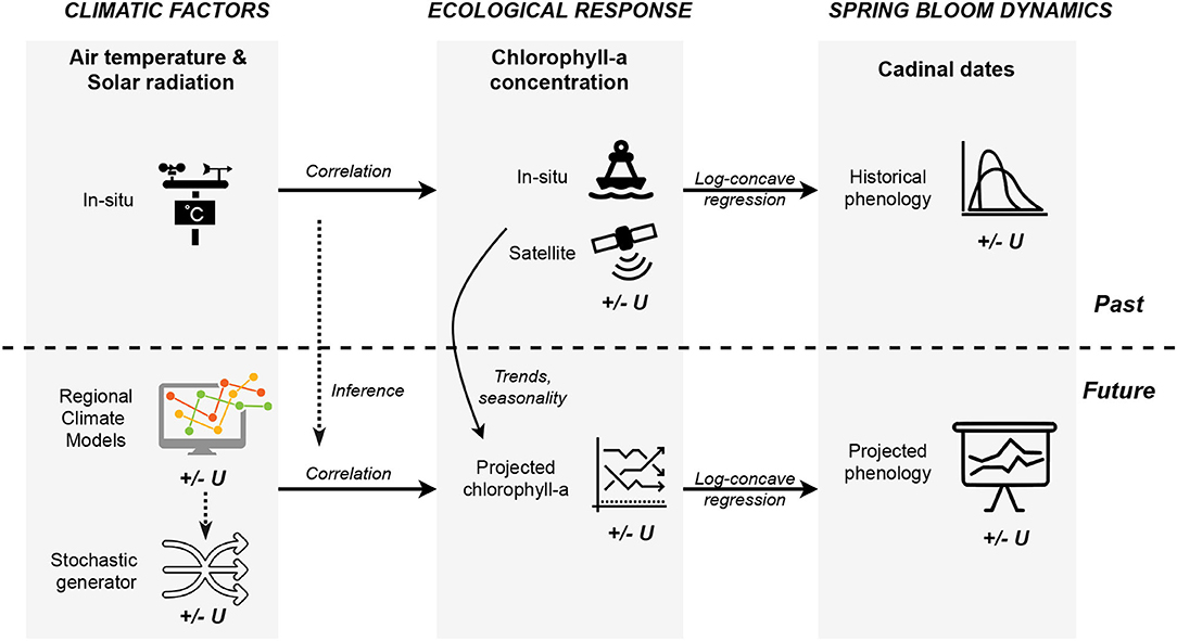
Figure 1. Methodological framework including three main elements with causal and temporal relations: (1) climatic factors, (2) ecological response, and (3) spring bloom dynamics.
2.1. Data Sources
This research is based on a multitude of data sources from sensors and numerical models of various types. The environmental and climate variables in this study are chlorophyll-a concentration, air temperature, and solar radiation. In order to investigate past trends and obtain the correlation between these variables, we make use of historical measurements, whereas to anticipate future climate change impacts, climate model outputs are used.
2.1.1. Chlorophyll-a Concentration Measurements
Available historical chlorophyll-a data includes field observations at Marsdiep Noord station (see Figure 2), from the Dutch Directorate-General for Public Works and Water Management (Rijkswaterstaat), covering more than 40 years from 1976 to 2018, but measured rather sparsely. To complement these field measurements, processed, and validated satellite observed chlorophyll-a concentration (extracted at the same location) was used from the Copernicus Marine Environment Monitoring Service (CMEMS) from 1997 to 2019 (see Figure 3). We should note that satellite observation of phytoplankton biomass in the Dutch coastal waters is complex since the chlorophyll-a signal may be mixed with the relative distribution of suspended matter and CDOM instead of phytoplankton biomass (Longhurst, 2007).
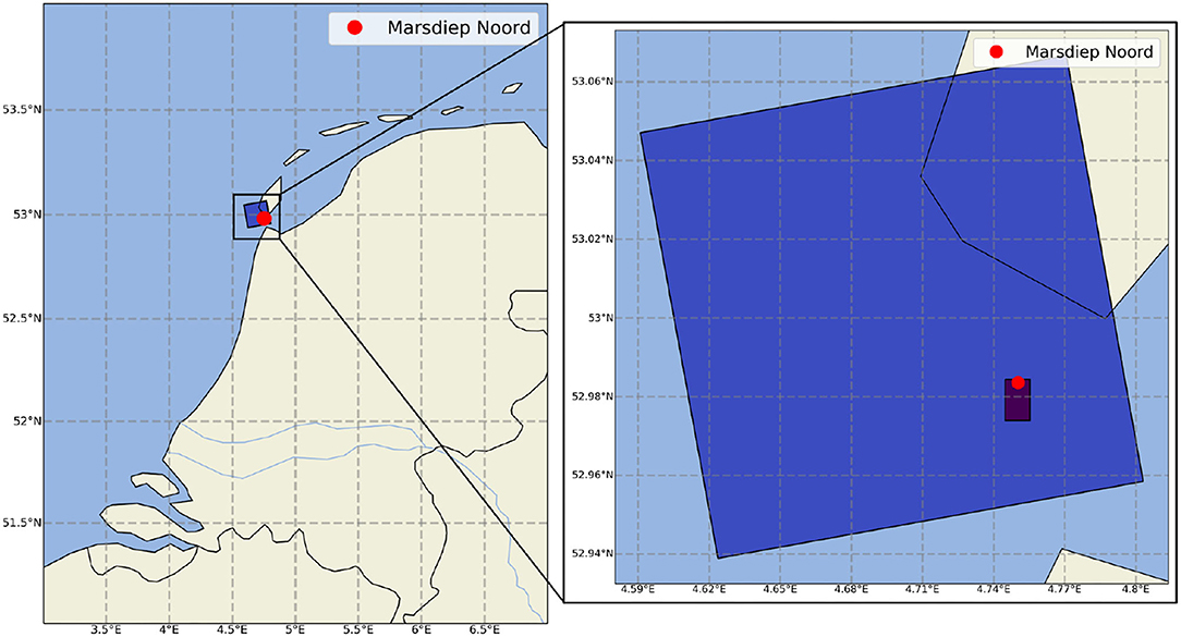
Figure 2. Location of the study area and the monitoring point together with the pixels of the matching Euro-CORDEX climate model output and CMEMS satellite measured chlorophyll-a.
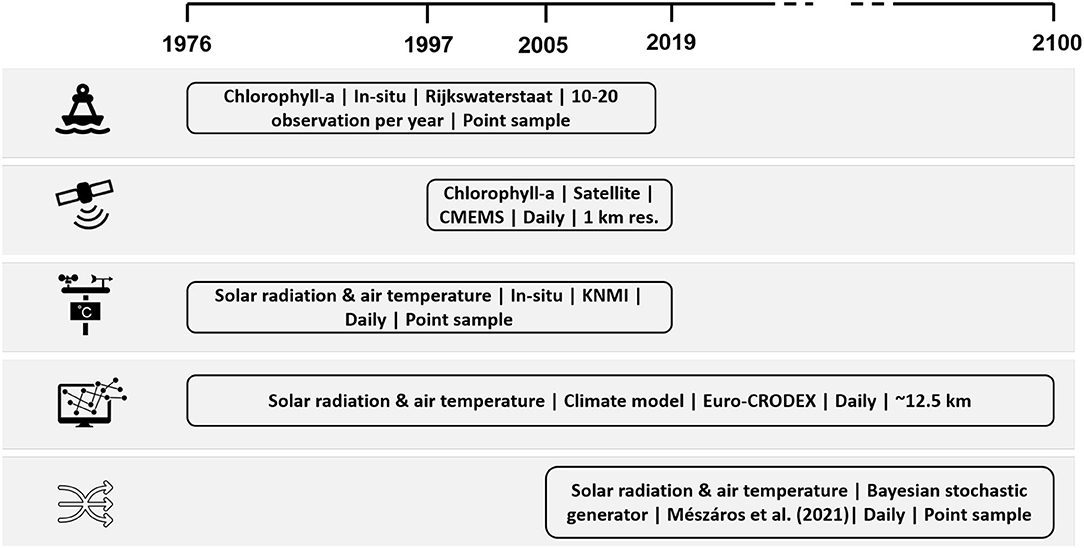
Figure 3. Overview of data sources. The description includes variable name, data type, data source, data frequency, and spatial resolution.
The specific product in use is the North Atlantic Chlorophyll-a, daily interpolated and reprocessed product with one km spatial resolution (OCEANCOLOUR_ATL_CHL_L4_REP_OBSERVATIONS_ 009_098). The satellite product is limited to the surface depth. This chlorophyll-a product is produced using multiple sensors (multi-sensor product), multiple chlorophyll-a algorithms and a daily space-time interpolation scheme (Saulquin et al., 2019). The interpolation scheme includes a combination of a water-typed merge of chlorophyll-a estimates and kriging interpolation method with regional anisotropic covariance models at the shore, as described in Saulquin et al. (2019). This product uses the Copernicus-GlobColor processor and it is obtained by merging the following sensors: SeaWIFS, MODIS Aqua, MODIS Terra, MERIS, VIIRS NPP, VIIRS-JPSS1 OLCIS3A, and S3B. For coastal waters the product uses the standard OC3-OC4 (Antoine and Morel, 1996; O'Reilly et al., 1998, 2000) and OC5 (Gohin et al., 2002) algorithms. The latest product validation results against in-situ measurements show an r2 of 0.73 with N = 11, 502 data points (Garnesson et al., 2020). For a more in-depth description of this satellite product the reader is referred to the QUality Information Document (QUID) (Garnesson et al., 2020).
The chlorophyll-a concentration seasonality from in-situ observation is shown in Figure 4A, and from satellite observations in Figure 4B. Naturally these data sources have different sampling methods and associated uncertainties. The in-situ observations are point samples taken by the Dutch national in-situ monitoring programme (MWTL) https://waterinfo-extra.rws.nl/monitoring/. It should be noted that the samples are taken close to the water surface, usually in the upper 3–5 m of the water column. These observations are often considered as ground truth and are the most reliable, however, in the case of chlorophyll-a concentration the temporal frequency of the observations is relatively low, around 10-20 observations per year. This amount of field observations poses a limitation to assess annual phytoplankton bloom cycles (Winder and Cloern, 2010). Thus, the more frequently sampled satellite images are also used to complement the in-situ measurements for a better assessments of bloom characteristics. This complementary data source is used noting that satellite derived chlorophyll-a is only available at the water surface (lack of vertical resolution), has a coarse 1 km resolution and suffers from algorithmic and interpolation errors, consequently having a higher level of associated uncertainty.
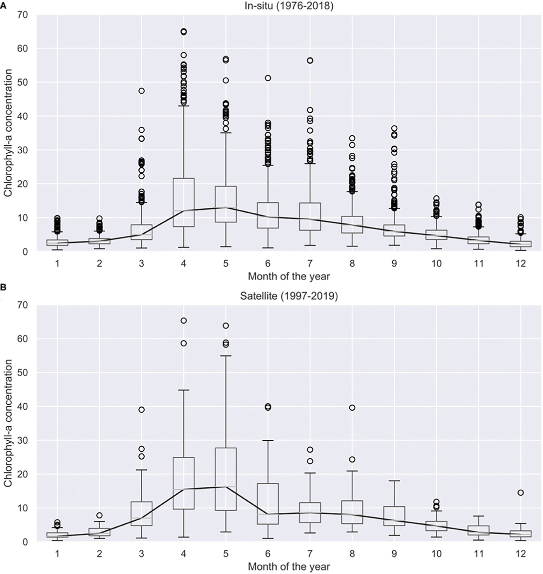
Figure 4. Historical chlorophyll-a concentrations measured in the Dutch Wadden Sea using in-situ data between 1976 and 2018 (A) and satellite images between 1997 and 2019 (B). Climatological median (solid black line) per calendar is also shown.
Since the two types of chlorophyll-a measurements describe the same underlying process, we propose a data fusion model to combine them. This data fusion model interlaces the in-situ and satellite observations into a single chlorophyll-a concentration signal, which is more complete then the individual observations and covers a longer time period. The data fusion model is described in section 2.2.
2.1.2. Solar Radiation and Air Temperature Measurements
The historical daily solar radiation and air temperature records are obtained at the nearest weather station (De Kooy) from the Royal Netherlands Meteorological Institute (KNMI) for the matching period (1976–2019). Apart from historical data, future projected values of air temperature and solar radiation are acquired from the high resolution 0.11° (~ 12.5 km) EURO-CORDEX Coordinated Regional Downscaling Experiment (Jacob et al., 2014), which uses the Swedish Meteorological and Hydrological Institute Rossby Centre regional atmospheric model (SMHI-RCA4). In order to produce various regionally downscaled scenarios, EURO-CORDEX applies a range of General Circulation Models (GCMs) to drive the above mentioned Regional Climate Model (RCM). In addition to the driving models, further scenarios are obtained by considering different socio-economic changes described in the Representative Concentration Pathways (RCPs). RCPs are labeled according to their specific radiative forcing pathway in 2100 relative to pre-industrial values. The EURO-CORDEX scenario simulations use the RCPs defined for the Fifth Assessment Report of the IPCC. In this study we include RCP8.5 (high), and RCP4.5 (medium-low) (van Vuuren et al., 2011) and four driving GCMs.
In the upcoming Sixth Assessment Report new scenarios and pathways will also be included, which are called Shared Socioeconomic Pathways (SSPs) (Abram et al., 2019). SSPs describe five alternative socioeconomic pathways (SSP1–SSP5) for future society enhancing the existing RCPs with socioeconomic challenges to adaptation and mitigation. Such socioeconomic challenges are population, economic growth, urbanization, or technological development for instance (O'Neill et al., 2017). It should be emphasized that SSPs are not replacing but complementing RCPs. In the Sixth Assessment Report the RCP-based climate projections and SSP-based socioeconomic scenarios are combined to achieve an integrative framework for climate impact and policy analysis (Abram et al., 2019). From the SSP scenarios SSP5-8.5 corresponds to RCP8.5 and represents the high end of the range of future forcing pathways, while SSP2-4.5 represents the medium part and corresponds to RCP4.5 (Abram et al., 2019).
Together the four different driving GCMs and two RCPs that are applied in this study provide us with an ensemble of eight future solar radiation and temperature trajectories. Since the RCM simulations are subject to climate model structural error and boundary errors from the driving GCMs (Navarro-Racines et al., 2020), they should be bias corrected before applying them in impact studies (Luo, 2016). For this reason, quantile mapping bias correction (Amengual et al., 2012) was applied using the RCM simulations for the reference period (1976–2005) and daily historical field measurements from KNMI for the same period, as described in Mészáros et al. (2021). The quantile-quantile mapping transfer functions were established for the reference period and separately for each RCM simulation. The transfer functions were then applied for the bias correction of each future projections (2006–2100) separately.
This ensemble of climate trajectories is used to simulate a range of possible phytoplankton seasonality shifts and the associated uncertainty described by the predictive distribution of the phytoplankton bloom cardinal dates. It should be noted that applying only eight climate projections reduces the ability to adequately resolve the unknown predictive distribution that one tries to estimate, hence, higher number of climate trajectories providing sufficient resolution in terms of probabilities is required (Leutbecher, 2019). Consequently, to better characterize uncertainties, an enriched set of climate change projections is employed. This set of air temperature and solar radiation projections was produced using a Bayesian stochastic generator (Mészáros et al., 2021), which builds on the above mentioned Regional Climate Model scenarios provided by the EURO-CORDEX experiment and generates further synthetic scenarios using a hierarchical Bayesian model. The generated ensemble of air temperature and solar radiation projections include 120 members and their statistical properties are similar to the input projections. Both the EURO-CORDEX and synthetic projections are shown for air temperature in Figure 5A and for solar radiation in Figure 5B. At this specific location we can observe a consistently increasing temperature trend over the twenty-first century and a slightly decreasing solar radiation trend. While increasing air temperatures are in line with expectations, decreasing solar radiation trends may need further explanation. The main cause of this negative trend is the fact that total cloud cover at this site is projected by EURO-CORDEX to increase, hence, limiting surface downwelling shortwave radiation. This is a region specific feature, and the difficulty of projecting cloud cover and solar radiation changes in coastal areas with sea-land-atmosphere boundaries, such as the study site, has been previously highlighted by Bartók et al. (2017), along with discrepancy between RCMs and their driving GCMs in their solar radiation projections over Europe.
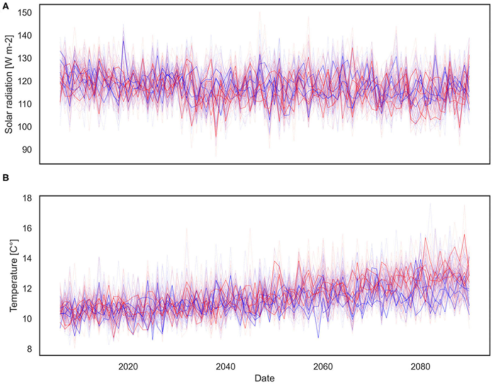
Figure 5. Eight EURO-CORDEX (darker solid line) and 120 generated synthetic (shaded dashed line) climate change projections for solar radiation (A) and air temperature (B), grouped by RCP scenarios (blue—RCP4.5, red—RCP8.5). Plot of the yearly averages based on the daily data.
2.2. Data Fusion of Chlorophyll-a Measurements
2.2.1. Statistical Model
In order to describe the chlorophyll-a concentration, we assume that there is a continuously evolving latent signal (Xt, t ∈ [0, T]) that satisfies the stochastic differential equation (sde)
The underlying idea is to model a stochastic process that is mean reverting (with strength α) toward the deterministic signal t ↦ μ(t). We will take μ to be periodic with period 1. We start off from a continuous time description as in-situ measurements are not collected at regular times. Observations can be of three types
1. Yi ~ N(Xti, ψ1);
2. Yi ~ N(Xti, ψ2);
3. .
This reflects having two types of measurements (in-situ and satellite) with different accuracies. Sometimes one measurement is obtained, sometimes the other one, and sometimes both are available. We take Yi to be the log of the measured concentration (component-wise) to ensure the model only predicts non-negative concentrations. While we acknowledge that there are other mapping functions to achieve non-negativity, taking the log of chlorophyll-a concentration is often used in practice (Campbell, 1995).
Assuming successive observations are obtained closely in time, i.e., Δi : = ti − ti−1 being small for all i, we have
where {ϵi}i is a sequence of independent standard Normal random variables. Ignoring discretization error, the resulting equation can be rewritten and combined with the observation scheme:
where Xi ≡ Xti. For numerical stability, it is better to discretize (1) using an implicit scheme on the deterministic part. This leads to the dynamical system
We write the model in state-space form, sticking to the notation in Särkkä (2013),
Here
and
Note that (2) specifies a linear Gaussian state-space model. The equation for Y is the observation equation, that for X the state-equation. We will parameterize ψ1, ψ2 by taking
where η ∈ (0, 1) is fixed and will get assigned a prior distribution supported on (0, 1). This reflects apriori knowledge that the in-situ measurements are believed to be more accurate. The in-situ chlorophyll-a observations are obtained from sampling campaigns (bucket water samples from a sampling jetty) and therefore considered as the true values (ground truth). While the satellite product is calibrated with many in-situ observations in the North Sea, it does not produce perfect match with the in-situ observations at the study location. Moreover, the number of satellite observations is much higher than the in-situ observations. This over-representation is counter balanced by the fusion model otherwise the reconstruction would be mostly determined by the satellite measurements.
We model the mean trend using the series expansion of the form
where K is fixed, and . This term allows us to account for a varying shape of the seasonal cycle. The functions φk are taken as follows: φ1 = 1[0, 1] and for j ∈ {1, …, J}
We take
which is the quadratic B-spline function scaled to have support [0, 1]. Note that φ0 is continuously differentiable. The hierarchical structure of the basis is exactly like the Schauder basis, but uses a smoother basic element than the traditional “hat”-function.
2.2.2. Inference
Let . Inference can be carried out by initializing θ and iterating the following steps (Robert and Casella, 2004):
1. conditional on θ, Y1, …, Yn, run the Forward Filtering Backwards Sampling (FFBS)-algorithm (see Appendix) to reconstruct X1, …, Xn;
2. draw from the posterior of θ, conditional on X1, …, Xn, and Y1, …, Yn (note that the likelihood is simple, once we know the latent path X1, …, Xn).
For updating parameters we use Gibbs sampling. Note that the updates for and ψ only depend on Y1, …, Yn, and updates for all other parameters only depend on X1, …, Xn.
• The updates steps for σ2 and ψ are trivial when using independent InverseGamma distributions as prior due to partial conjugacy.
• For we assume the Unif(0, 1)-prior. A Metropolis-Hastings step is implemented where we use random-walk type proposals (Robert and Casella, 2004) of the form
which implies that the proposal ratio equals
Note that , where Z ~ N(0, 1).
• For updating α we use a Metropolis-Hastings step of the form .
• The “full” conditional density for ξ is proportional to
where
This is proportional to
with
Hence, the update step for ξ boils down to sampling from a multivariate normal distribution with precision and potential vector σ−2v (the potential vector is the product of the precision matrix with the mean vector).
Details on the prior specification: for both σ2 and ψ we took (independently) InverseGamma priors, parameterized with shape and scale, with both parameters equal to 0.1. For α we took the Exponential distribution with mean 10. We took and tuned the step-sizes τψ and τα such that the corresponding random-walk Metropolis-Hastings steps were accepted with probability in between 25 and 50%. In the series expansion we took a fixed value for K = 5. We took η = 658/8, 005, which is the ratio of the in-situ and satellite measurements.
2.3. Long Term Projection Using Bayesian Structural Time Series Models
After the fused historical chlorophyll-a concentration signal has been derived, it is used to train the time series model for scenario analysis. It was previously argued that variability in the spring bloom dynamics occur due to changing environmental conditions. Consequently, apart from historical trends and seasonality in the observed chlorophyll-a concentration time series, projected solar radiation and air temperature are also used to drive future chlorophyll-a concentration trajectories. These simulated trajectories are then utilized to extract the bloom characteristics applying the feature extraction methodology described in section 2.4.
In this study an existing Bayesian structural time series modeling framework is customized to our purpose, which is the Prophet forecasting model (Taylor and Letham, 2017). This is a decomposable time series model with trend, seasonality, and additional regressor component, as well as error term as the main model components:
where, at time t, y(t) is the response variable (chlorophyll-a concentration), g(t) is a piecewise linear trend model, l(t) is a linear component representing seasonality and additional regressors, and ϵ(t) is the error term (independent and identically distributed noise). In order to avoid negatively predicted values, the natural logarithm of the response variable was taken in the model, and the prediction was then transformed back to its original scale by using the exponential function. An advantage of the Prophet model is that it can handle irregular intervals, which is important as our fused chlorophyll-a observations are not regularly spaced. Prohpet is similar to other decomposition based approaches to time-series forecasting except that it uses generalized additive models instead of a state-space representation to describe each component. Using state space models would offer a more generic model formulation, whereas this approach explicitly models features common to the chlorophyll-a time series at hand, such as multi-period seasonality. The structural time series model could alternatively be put into state-space format, but rewriting it into that form would not alter the results.
Bayesian structural time series models possess further key features for modeling time series data that are favorable for long-term chlorophyll-a scenario analysis studies. The main feature is uncertainty quantification, as they allows us to quantify the posterior uncertainty of the individual components, control the variance of the components, and impose prior beliefs on the model. This is crucial as uncertainties increase over time in the future, especially in long-term projections. The second key feature is transparency, since the model is decomposed into simple time series components, which can be visually inspected. Moreover, they do not rely on differencing or moving averages, which make them more transparent than other autoregressive moving average models. The third key feature is the ability to incorporate regressors (covariates) as explanatory variables in the model. This feature is beneficial to include climate change impacts on chlorophyll-a trajectories from solar radiation and air temperature.
Here we briefly introduce the model without aiming completeness; for the full model formulation the reader is referred to Taylor and Letham (2017). We use a piecewise linear model with a constant rate of growth and change points. Suppose there are S change points, over a history of T points, at times sj, j = 1, …, S. We define a vector of rate adjustments δ ∈ ℝS, where δj is the change in rate that occurs at time sj. The rate at any time t is then the base rate k, plus all of the adjustments up to that point, which is represented by a vector a(t) ∈ {0, 1}S such that
The piecewise linear trend model with change points is then
where k is the growth rate, a(t) is a change point indicator as defined above, δ is the vector of rate adjustments, m is the offset parameter, and to make the function continuous, γj is set to −sjδj. We employ the following prior on δ = (δ1, …, δS).
where τ controls the flexibility of the model in alternating its rate. While the model automatically detects change points and allows the trend to adapt appropriately, we have control over the trend flexibility by adjusting the strength of the sparse prior using the change point prior scale τ. In this application trend flexibility is significantly reduced by decreasing the change point prior scale to one fifth of its default value. The value was fined tuned by balancing between the training error (which is lower with more flexibility) and the prediction error, while keeping the width of the projected uncertainty interval reasonable.
When the model is used for forecasting, the trend has constant rate and the uncertainty in the forecast trend is estimated. Future rate changes are simulated that emulate those of the past. In a fully Bayesian framework this can be done with a hierarchical prior on τ to obtain its posterior. In long-term projections, which is our purpose, one of the most influential factors is the uncertainty in the future trend. In this model, the uncertainty in the forecast trend is estimated by assuming that in the future the same average frequency and magnitude of rate changes will occur as observed in the past:
Once λ has been inferred from the data, we use this model to simulate possible future trends and to compute uncertainty intervals. Due to the assumptions in the trend forecasting (matching historical frequency and magnitude) the trend intervals may not be exact, nevertheless they provide an indication of the level of uncertainty and also reveals trend model overfitting.
In the seasonality model we approximate seasonal effects with a standard Fourier series expansion with chosen periodicity P, and Fourier order n. The seasonality model is:
In this model the following periods are used, P = 3652.5 for decadal periodicity, P = 365.25 for yearly periodicity, P = 182.625 for half-yearly periodicity, and P = 91.3125 for quarterly periodicity (in days). The Fourier order was chosen as N = 10 after tuning such that under-fitting and over-fitting is avoided by minimizing the test error. The linear component then becomes
where is a matrix of seasonal components s(t) and additional vectors of regressors, while includes the 2N parameters of the Fourier series expansion and the R regression coefficients of the additional explanatory variables. The following β ~ N(0, σ2) prior is imposed independently on each component of β. By default the linear component of the model only contains features for modeling seasonality but through specifying covariates (“regressors”) we can include additional arbitrary vectors to X(t) whose regression coefficients will be inferred. Combining the trend, seasonality, and error components the final model becomes:
In order to construct an appropriate structural time series model, the selection of model components was facilitated by exploratory analysis steps, such as seasonal shape extraction, investigating the correlation of explanatory and response variables (Figure 6), produce periodogram and wavelet analysis to explore periodicity, and perform time series decomposition. Apart from chlorophyll-a, the solar radiation regressor data is also log transformed, since that produces a correlation structure to log chlorophyll, which is closer to linearity (see Figure 6). The temperature data could not be log transformed as it contains negative values. The continuous wavelet power spectrum revealed a persistent 12-month periodicity, which explained the largest amount of variability over the sampling period, while the rest of the variability is attributed to 6 and 3 month periodicity. This is in line with previous research findings of wavelet analysis for the same observation station (Winder and Cloern, 2010).
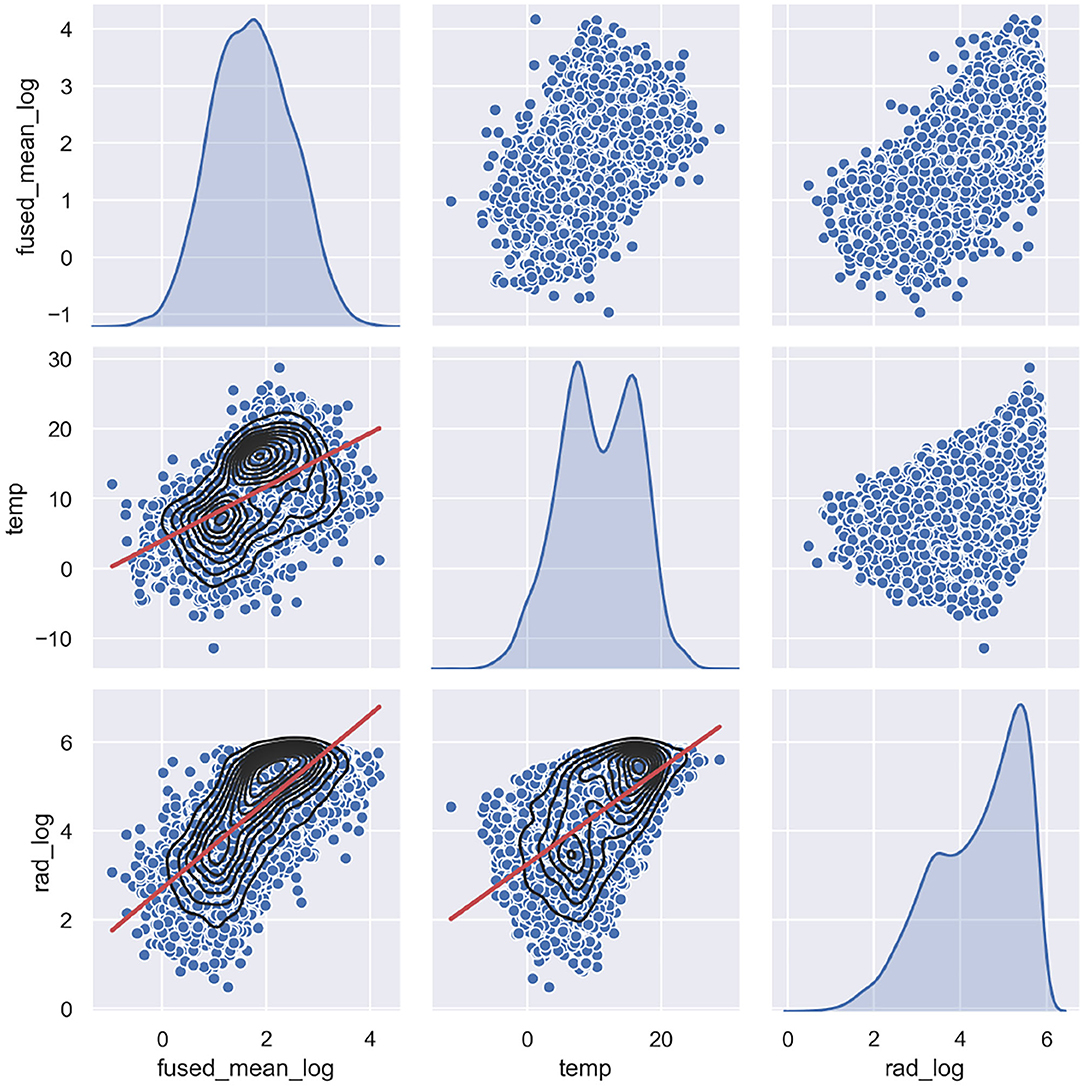
Figure 6. Pair plots of the log transformed response variable (fused chlorophyll-a), and the explanatory variables (log transformed radiation and temperature). Scatter plots are shown together with Kernel Density Estimates (black) and linear regression (red).
In the current structural time series model implementation the following components are used. Linear trend with change points (change point prior scale is defined), multi-period seasonality: decadal, yearly, half-yearly, and quarterly (periodicity, Fourier order, and prior scale are defined), as well as four additional regressors (air temperature, solar radiation, and their lag1). It should be noted, that adding more than lag1 of the regressors did not improve the prediction further. The parameter inference can be either done by optimization, using Limited-memory Broyden-Fletcher-Goldfarb-Shanno algorithm (L-BFGS) to find a maximum a posteriori estimate, or through full posterior inference to include model parameter uncertainty in the forecast uncertainty.
2.4. Tracking Phytoplankton Spring Bloom Dynamics
In order to track phytoplankton spring bloom dynamics, the last step of the methodological framework focuses on deriving spring bloom metrics obtained from the chlorophyll-a concentration time series. We must emphasize that uncertainty in the previous methodological steps (data fusion and long term projection) is being propagated to the estimates of cardinal dates and bloom magnitude. Although efforts have been dedicated to quantify these uncertainties, propagated uncertainty carries implications for the accuracy of the calculated cardinal dates.
Several existing methods are available to characterize phytoplankton blooms. Ji et al. (2010) provides an exhaustive list of timing indices for quantifying phytoplankton phenology with advantages and disadvantages. These can be classified as biomass-based threshold methods, rate of change methods, and cumulative biomass-based threshold methods (Brody et al., 2013). One might use the number of consecutive days that exceed a given threshold (elevated assessment level) defined by the literature. In the case of Dutch coastal waters this is around 12–15 and 22–24 mg/m3 for the Wadden Sea (Peters et al., 2005). Alternatively, a low-pass method could be used for determining the start of the bloom (Wiltshire et al., 2008), which is a temporal averaging algorithm acting as a low-pass filter, reducing the short-term fluctuations. Philippart et al. (2010) suggested using the date of the maximum and minimum values of daily change rates in the interpolated chlorophyll-a concentrations for the timing of the annual onset and breakdown of the phytoplankton bloom. The timing of the bloom can also be represented by another quantity, the center of gravity (COG) of the carbon content within the typical spring bloom period (Hjerne et al., 2019). Another possibility to characterize the spring bloom is to derive the cardinal dates of the mass development (Rolinski et al., 2007). The cardinal dates are the beginning of the spring phytoplankton mass development, the maximum of the spring bloom (bloom peak), and the end of the spring mass development. Mathematical methods of describing cardinal dates were proposed by Rolinski et al. (2007), such as finding the points of inflexion in the smoothed, log transformed, and differenced (1-week lag) data, deriving them from four linear segments (constant–increasing–decreasing–constant) fitted to the logarithmic values, or extracting the cardinal dates from the quantiles of a fitted parametric function (Weibull function). Similarly, Lewandowska and Sommer (2010) transformed phytoplankton biomass according to standard normal variation and took the first and third quartiles as cardinal dates, the beginning and the end of the spring bloom, respectively.
Several of the above mentioned methods (or listed by Ji et al., 2010) cannot properly deal with bi-modal data (require separation of the spring bloom) or large fluctuations in amplitude, some methods need parametric fitting (e.g., Vargas et al., 2009), and most methods cannot deal with noisy data, hence require smoothing to pre-process the seasonal data before deriving the cardinal dates. As summarized by Ji et al. (2010) if the seasonal time series is uni-modal, from densely sampled and without noise, most methods will perform well. This is rarely the case, unless the data is interpolated and denoised. If that is not the case, more flexible approaches perform better which use less assumption on distribution patterns. For this reason to track long term changes in phytoplankton spring blooms we propose to derive the cardinal dates using a non-parametric shape constrained method, namely log-concave regression (Groeneboom et al., 2001; Groeneboom and Jongbloed, 2014; Doss, 2019). Log-concave regression meets this flexibility requirement as it does not require any tuning parameters and can be directly applied on the annual bi-modal time series without any pre-processing. Consequently, our proposed method is less sensitive to bloom amplitude, missing data, and observational noise.
In summary, determining a mode of a unimodal (part of a) function, sometimes called “bump hunting” is classically done using smoothing techniques, assuming some level of smoothness (which is reasonable) of the function. The advantage of using log-concave regression compared to techniques based on smoothing, is that it does not require tuning parameters (such as bandwidths) that heavily influence the outcome of the analysis. An alternative method one could use, would be unimodal regression, where no smoothness is used at all, resulting in discontinuous unimodal step functions as estimate of the regression function. The large class of log-concave functions contains unimodal functions that are continuous. Moreover, estimation of these can be done in a stable manner.
In order to track long term changes in phytoplankton spring blooms we propose to derive the cardinal dates using a non-parametric shape constrained method, namely concave regression (Groeneboom et al., 2001; Groeneboom and Jongbloed, 2014; Doss, 2019). The concave or convex regression setup for a data set of size {n :(xi, yi) : i = 1, …, n} where x1 < x2 < … < xn is the following:
for a concave function r0 on ℝ, where {ϵi : i = 1, …, n} are independent and identically distributed random variables and Yi is the log chlorophyll-a concentration. Then, we apply concave regression on the log chlorophyll-a concentration data. We assume that the target of the estimation, r0 : ℝ → ℝ, is concave. Writing for the set of concave functions on ℝ, the least squares estimate of r0 is
Utilizing this concave regression setup, the following two methodological steps are taken to identify the spring bloom cardinal dates (see Figure 7). The cardinal dates are the spring bloom beginning (B), -peak (P), and -end (E) dates expressed as the day of the year.
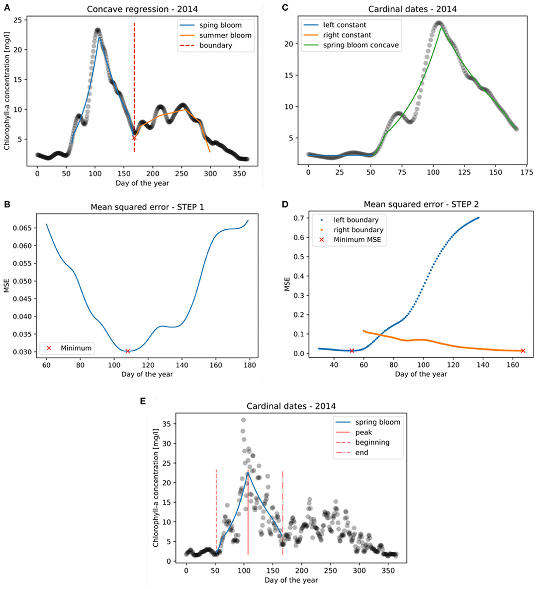
Figure 7. Steps to derive the cardinal dates of phytoplankton spring blooms: (1) Determining the boundary (tb) for isolating the spring bloom (A,B), and (2) concave regression to spring bloom (C,D). The cardinal dates of the spring bloom are shown in (E).
2.4.1. Isolating the Spring Bloom
We take yearly time series of log chlorophyll-a concentrations (yt), and assume that it is bi-modal separated by a boundary point tb. In order to reduce computation time of the first step, we omit the first 2 months (t1 = 60) and last 2 months (t2 = 300) of the dataset since we know that the boundary that separates the spring and summer bloom will not be found there. It should be noted that omitting a portion of the yearly time series is only done in the first step during the identification of the boundary point. In the latter step, during the derivation of the spring bloom cardinal dates all dates on the “left side” of the boundary point are used . Omitting a portion of the yearly time series is optional. Then we fit Φ(t) on the data:
where φtb(t) is the concave regression of (xi, yi) : xi ≤ tb on [t1, tb], the “left side,” and is the concave regression of (xi, yi) : xi > tb on [tb + 1, t2], the “right side.” Therefore, both φtb(t) and are concave. The optimal boundary is found where the mean squared error of Φ(t) is minimal:
This process of determining the boundary of spring and summer bloom is visually depicted in Figures 7A,B.
2.4.2. Derive Cardinal Dates of the Spring Bloom
After finding the boundary () only the spring bloom (“left side”) of the data is considered for further analysis where . Then we take a continuous function Φ*(t) which is defined as follows:
where cl and cr are constant and φ(t) is the concave regression of (xi, yi) : tl < xi ≤ tr. The points where the left constant function ends and the right constant function starts (tl and tr) will become the beginning and the end of the bloom (cardinal dates B and E). The third cardinal date, the peak of the bloom, is where φ(t) takes its maximum. The points tl and tr are found where the mean squared error of Φ*(t) is minimal:
This final methodological step to identify tl and tr is shown in Figures 7C,D. Finally, the cardinal dates together with the concave regression and the chlorophyll-a time series (transformed back to original values by taking their exponential function) are depicted in Figure 7E.
3. Results
3.1. Fused Chlorophyll-a Concentration Signal
The fused chlorophyll-a concentration signal, together with satellite observations, is depicted in Figure 8A and with in-situ observations in Figure 8B. One can observe that the fused signal almost perfectly follows the in-situ (“water”) observations over the period in which only that type of measurements are available. From the moment that both in-situ and satellite date are available (1998), the fused signal lies between the two types but being closer to the in-situ observations according to the model formulation, since we have higher confidence in the field data. This is also reflected in the quantile-quantile plot and scatter plot of the fused signal compared to the in-situ data in Figures 8C,D, which lies almost perfectly on the diagonal, whereas the plot of the fused signal against the satellite observations deviates more from the diagonal. This enhancement of the historical chlorophyll-a signal has benefits for the projection step. Since the long-term projection is largely based on the observed correlations, if the input chlorophyll-a concentration time series is less accurate the statistical model will misrepresent the processes.
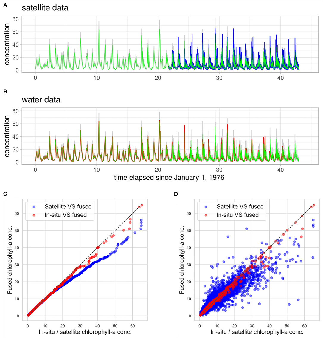
Figure 8. Data fusion results. The mean fused chlorophyll-a concentration signal (green) with uncertainty (gray) compared with satellite observations (blue) in (A), and in-situ “water” observations (red) in (B). Quantile-quantile plot of the fused signal compared to both in-situ and satellite observations in (C) and scatter plot in (D).
3.2. Long Term Chlorophyll-a Projection
The Bayesian structural time series model (introduced in section 2.3) was trained (1976–2010) and tested (2010–2018) on the fused chlorophyll-a concentration signal and the historical measured solar radiation and air temperature data. Figure 9 visually depicts the validation of the in-sample forecast (1976–2010) and the forecast (2010–2018) against the fused data. The figure shows that most measurements (75%) lie within the predictive uncertainty band, indicating the model's reliability. The scatter plot of predictions is shown in Figure 10 whereas the performance metrics can be found in Table 1.
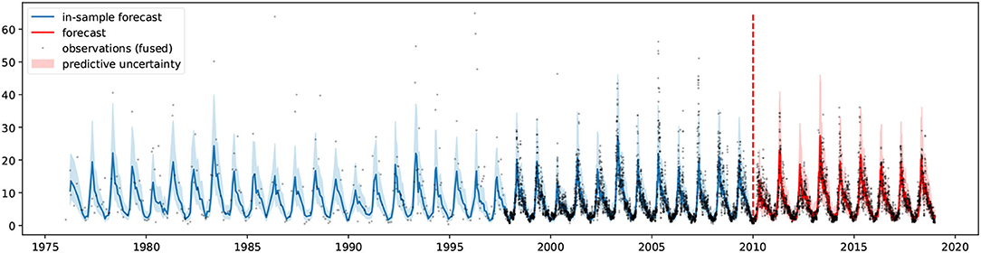
Figure 9. Time series forecasting validation against fused observations. Model fit between 1976 and 2010 (blue) and forecast between 2010 and 2018 (red). Predictive uncertainties in shaded area.
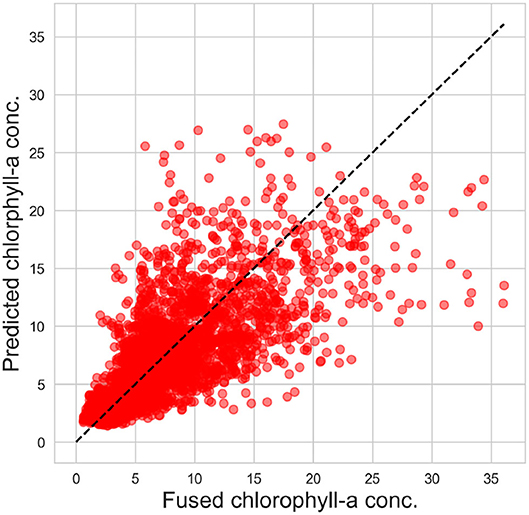
Figure 10. Scatter plot of predicted chlorophyll-a concentration against fused observations. Model forecast between 2010 and 2018 with N = 3,287 data points.
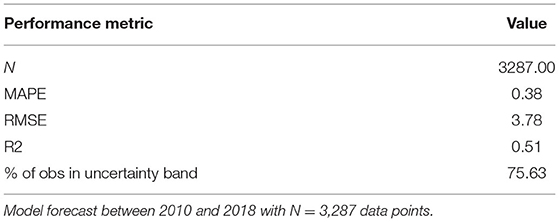
Table 1. Time series forecasting validation metrics against fused observations.
While long-term data driven chlorophyll-a concentration prediction for climate impact assessment is not widespread, there have been few studies conducted on both inland water systems (Cho et al., 2018; Keller et al., 2018; Liu et al., 2019; Luo et al., 2019) and marine systems (Irwin and Finkel, 2008; Blauw et al., 2018; Krasnopolsky et al., 2018; de Amorim et al., 2021) that performed short term predictions. Blauw et al. (2018) predicted chlorophyll-a in the North Sea at different sites applying Generalized Additive Models (GAMs) with accuracies (R2 values) ranging from 0.25 to 0.51 for hourly time scale, 0.15–0.22 for daily time scale, and 0.27–0.63 for bi-weekly time scale. Higher accuracy (R2 = 0.83) was obtained in the North Atlantic, using a spatial GAM to predict month-to-month variation (Irwin and Finkel, 2008) or in a recent study by de Amorim et al. (2021) where an R2 value of more than 0.7 was achieved for a longer-term prediction (multi-year) with three different algorithms: Support Vector Machine Regressor (SVR), Random Forest, and Multi-layer Perceptron Regressor (MLP). SVR performed the best (R2 = 0.78) with 17 predictor variables. Similar accuracies (R2 values) were achieved in short-term prediction studies for lakes or reservoirs using Random Forest algorithm on monthly (0.2–0.6) and daily (0.6–0.8) data (Liu et al., 2019), as well as using Multiple-Layer Perceptron Neural Network (MLPNN) and Adaptive Network-based Fuzzy Inference System (ANFIS) 0.52–0.85 (Luo et al., 2019). In comparison with these studies, we conclude that our model has acceptable accuracy, especially considering that we predict on a daily scale and 8 years ahead, while most of the cited work focuses on much shorter prediction time frame. It should be noted that model comparability with other studies is hampered not only by the differences in ecosystem types (fresh water or open ocean instead of coastal waters) but also due to the fact that the predictor variables differ, and so as the experimental setup such as data splitting strategies, and prediction time frames.
After the calibration of hyperparameters and initial validation, the time series model was retrained using the entire historical period (1976–2018), to better capture historical trends, and used for long-term chlorophyll-a concentration projection (2019–2089). Since the model contains log transformed solar radiation and air temperature as regressors, they need to be provided for the entire projection period. Consequently, after 2019 the bias corrected climate change projections are applied instead of the field observations. Given the numerous generated climate change projections (120 were used), the same number of future chlorophyll-a concentration trajectories were simulated, as shown in Figure 11. One can observe that the predictive uncertainty increases over time as we get farther from the projection start date. This predictive uncertainty originates from the trend component as explained in section 2.3, and the modeling choices (e.g., changepoint prior scale) will influence it. We should emphasize that such long term projection is only a simplified approximation of the future chlorophyll-a signal, which follows a piecewise linear trend and continues to repeat its multi-seasonal behavior, learnt from the past data, moreover includes linear effects of the two climate variables. These assumptions guarantee fast computation time, thus allowing numerous simulations for uncertainty quantification, which is the objective of this study. Nonetheless, it does not replace complex physically-based numerical models that are capable of simulating a wide range of ecological processes.
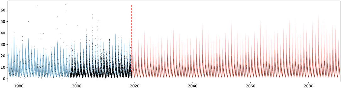
Figure 11. Long term chlorophyll-a concentration time series projection with radiation and temperature explanatory variables from generated climate projections (based on EURO-CORDEX). One hundred and twenty solar radiation and air temperature projection scenarios were used to produce the 120 chlorophyll-a trajectories. Model fit between 1976 and 2018 (blue) and projection between 2019 and 289 (red). Predictive uncertainty in shaded area.
3.3. Changes in Phytoplankton Bloom Dynamics
The feature extraction step to derive the spring bloom cardinal dates (see section 2.4) is first applied to the mean fused chlorophyll-a data to obtain the historical changes in spring bloom dynamics. Unfortunately, the cardinal dates could only be derived starting from 1998. This is due to the fact that between 1976 and 1998 only in-situ measurements were available which had a sparse temporal sampling frequency (10–20 per year). As previously argued, this number of yearly data points is insufficient to extract the cardinal dates. The historical phytoplankton bloom dynamics from 1998 to 2018 is depicted in Figure 12. The figure displays the three cardinal dates (beginning—green, peak—red, end—blue), the bloom duration (shaded blue area), and the bloom duration anomaly from the long-term mean bloom duration (bar chart). It can be observed that for certain years (2002, 2012, 2013) the bloom peak and bloom end cardinal dates lie very close to each other. These instances were visually confirmed. It was found that for 2002 and 2012 the feature extraction algorithm was accurate as a fast decay followed the bloom peak. On the other hand, in 2013 there was visibly no spring bloom observed, only a dominant summer bloom. This led the algorithm to falsely identify the spring bloom peak and end. This finding suggests that years where no spring bloom is observed should be removed from the dataset prior to applying the spring bloom cardinal detection algorithm. A possible extension of the method could be to report the type of seasonality (spring bloom, summer bloom, bi-modal, no bloom) (González Taboada and Anadón, 2014) since changes in the type of seasonality are of interest, nevertheless, this is not part of the current implementation.
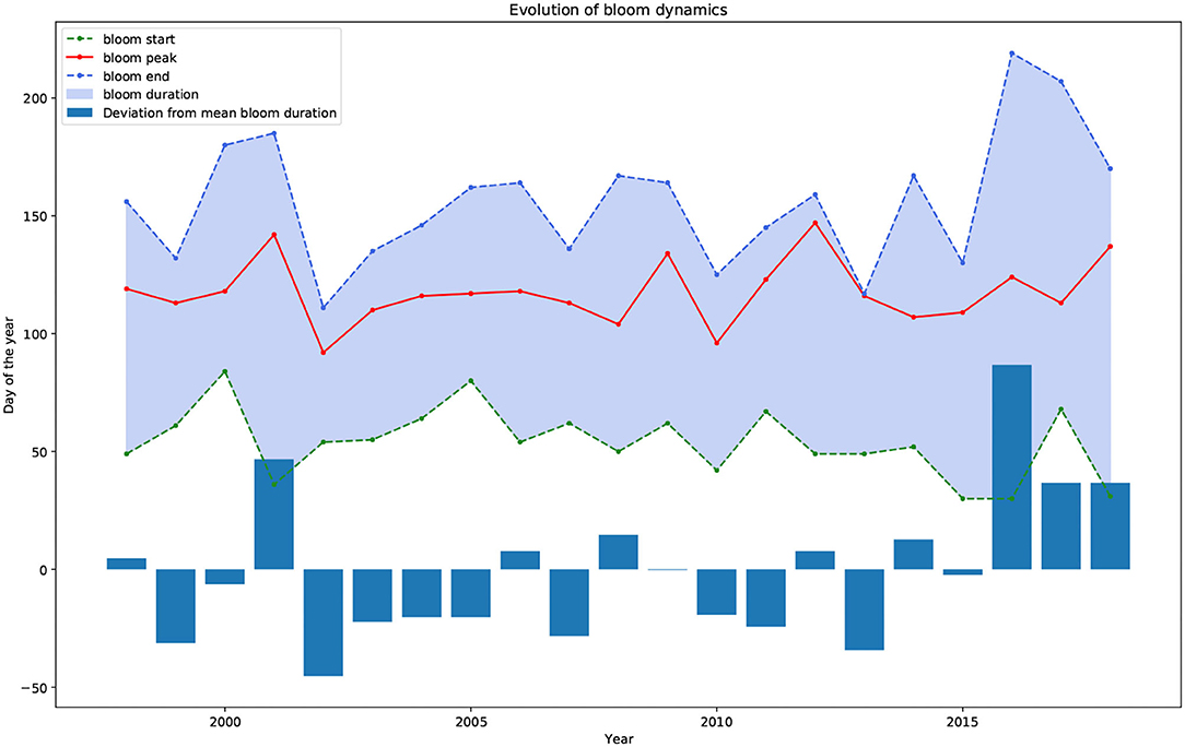
Figure 12. Historical spring bloom cardinal dates (beginning—green, peak—red, end—blue) and bloom duration (shaded blue area). The bar chart shows the yearly deviation (anomaly) from the long-term mean bloom duration.
The feature extraction steps are then repeated on the projected future chlorophyll-a concentration between 2019 and 2089. The projected future spring bloom cardinal dates are depicted as boxplots in Figure 13A and as histograms in Figure 13B. The results indicate a relatively small variation, ~ 6 days, in the projected bloom peak timing (see Figure 14B), while a much higher level of uncertainty is observed for the bloom beginning, ~ 25 days, (see Figure 14A) and end timing, ~ 20 days (see Figure 14C). Bloom beginning and -peak resemble normal distributions, in the case of the bloom peak with a lower variance (higher peakedness). On the other hand, the bloom end resembles a right skewed log-normal distribution with relatively heavy tale due to the high number of outliers.
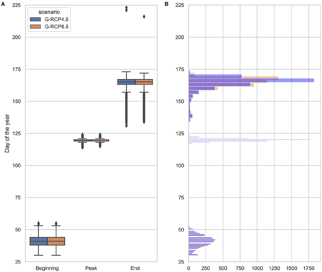
Figure 13. Range of projected future bloom cardinal dates (A) and their distributions (B) under 120 generated radiation and temperature projections (based EURO-CORDEX) (2019–2089). The statistics are grouped based on the generated projections corresponding to RCP scenarios (G-RCP4.5 and G-RCP8.5).
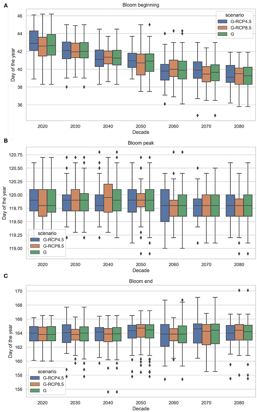
Figure 14. Projected future phytoplankton spring bloom beginning (A), peak timing (B), and end (C) under generated (G) radiation and temperature projections (based EURO-CORDEX) (2019–2089). The cardinal dates are grouped based on all generated projections (G), and generated projections corresponding to RCP scenarios (G-RCP4.5 and G-RCP8.5).
The bloom beginning is projected to slightly but consistently shift earlier, resulting in longer bloom duration toward the end of the century (see Figure 15A). The earlier spring bloom as an effect of climate change is in line with previous findings by Lewandowska and Sommer (2010) and Winder et al. (2012) in laboratory trials (mesocosm experiments), by Desmit et al. (2020), Hjerne et al. (2019), Philippart et al. (2010), and Edwards and Richardson (2004) using historical data, or by Friocourt et al. (2012) using numerical (hydrodynamic and ecological) prediction models forced by future climate change scenarios. Many of these studies found an even higher rate of spring bloom forward shift but in our case the accelerating effect of temperature rise might be moderated by the decreasing solar radiation trend. Despite the considerable uncertainty in the bloom end timing, no apparent trend can be observed. We emphasize that the actual day of the year of the derived cardinal dates may not be comparable to other findings in literature, since we used another method to obtain these cardinal dates. Thus, the projected trends and uncertainties carry the most value. We should also point out that the projected earlier spring blooms may not be a simple climatic response but could be the result of complex processes (physical and non-physical). Further investigation of these processes is necessary to fully understand the underlying mechanisms causing shifts in phytoplankton dynamics (Hjerne et al., 2019).
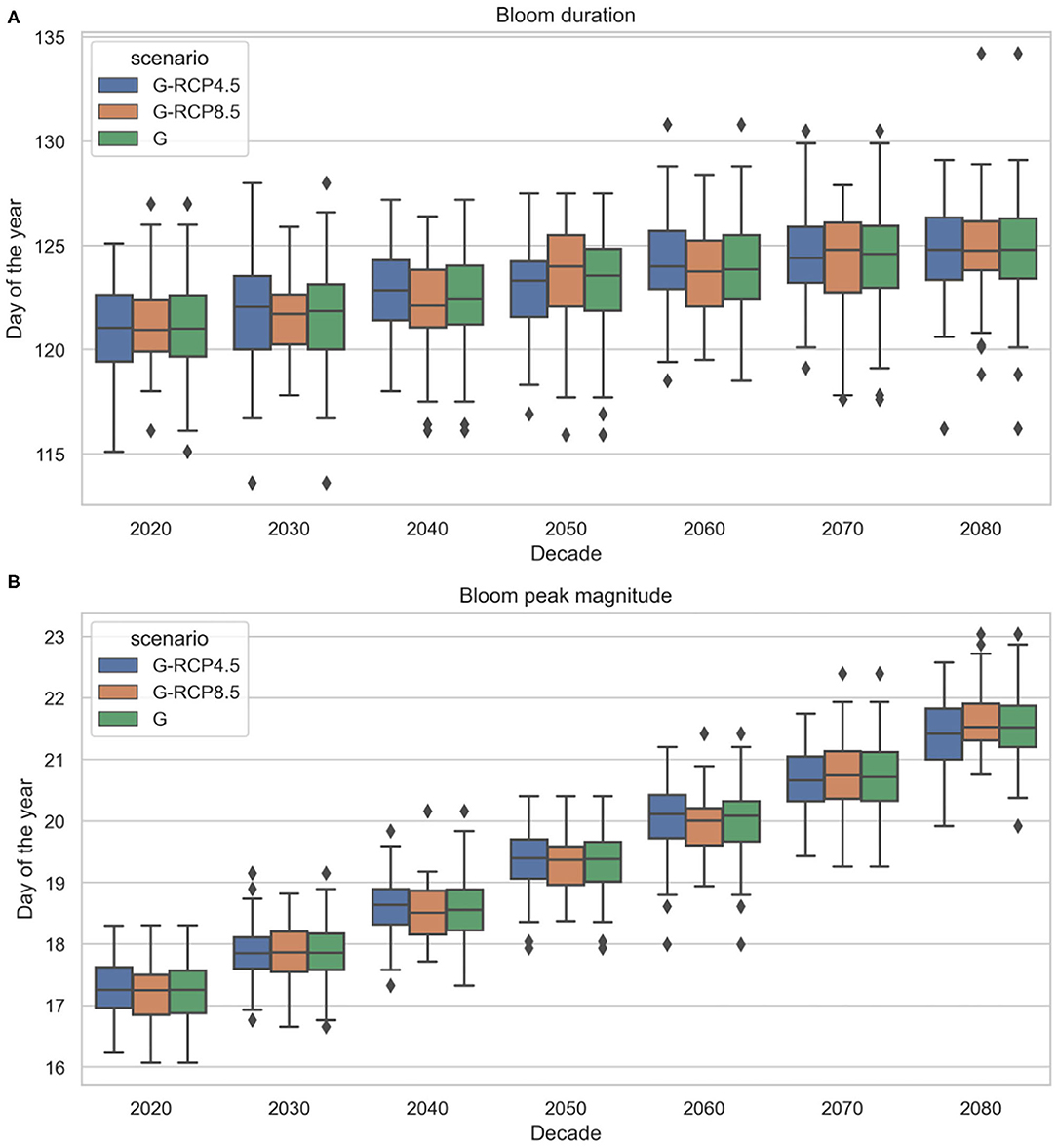
Figure 15. Projected future phytoplankton spring bloom duration (A) and peak magnitude (B) under generated radiation and temperature projections (based EURO-CORDEX) (2019–2089).
Apart from the cardinal dates, the chlorophyll-a concentration magnitude was also investigated. As Figure 15B shows, at the end of the twenty-first century higher spring bloom peak magnitude can be expected. Considering the ensemble mean values, a 0.4%year−1 trend is projected. This trend magnitude is comparable with the latest findings on chlorophyll-a historical trends in the North-West Shelf regions (0.4–0.96% year−1) Hammond et al. (2020), noting that this estimate was considering offshore marine waters, not coastal zones. It is also comparable to Xu et al. (2020) who found nearly 20–30% chlorophyll increase in the same study area between 1987 and 2012. Various numerical studies using climate models also project moderate increase in daily mean net primary production between 1980–1999 and 2080–2099 in the shallower southern North Sea (Holt et al., 2014, 2016; Pushpadas et al., 2015). We must emphasize that increasing chlorophyll concentration due to climate change is highly region specific (only occurring in some coastal areas) and very much debated (Xu et al., 2020). In fact, some studies only report shift in spring bloom timing and species composition, but not in magnitude. In our study the projected positive trend is most probably driven by the linear trend component of the time series model and the rising air temperature as regressor, which have positive correlation to chlorophyll, based on the historical data. It should be noted, that in reality the correlation between air temperature and chlorophyll-a is non-linear and seasonally varying, moreover, it is different on a species or aggregate level. As the time series model could not incorporate non-linear correlations, it is assumed linear, hence, simulated interactions are only approximations of the real conditions. Nevertheless, in the season of interest (spring), when air temperature and solar radiation values did not reach their peak, this correlation is positive and the linearity assumption is a good approximation (see Figure 6). Furthermore, with chlorophyll-a concentration as a proxy we aim to describe aggregate level response, rather than species level response. We also emphasize that bloom magnitude is heavily influenced by nutrient concentration in the mixed layer depth (Sverdrup, 1953; Behrenfeld, 2010). Although nutrient concentration was not used as an explanatory variable in this study we may expect that the correlation between air temperature and chlorophyll-a captured in historical data may include indirect effects such as thermal stratification, which influences nutrient availability in the mix layer depth.
The projected cardinal dates in Figures 13–15 are also grouped based on the generated projections corresponding to RCP scenarios. One observed difference is that in the last two decades bloom peak magnitudes are somewhat higher for RCP8.5. Perhaps counter intuitively, no other structural differences are visible between the RCP scenarios. The similarity between projected cardinal dates corresponding to RCP scenarios could be attributed to few reasons. Firstly, we must investigate the differences in solar radiation and air temperature projections between the RCP scenarios from Euro-CORDEX. As Figure 5 depicts, these differences for solar radiation are not apparent. For air temperature projections we see similar behavior until the end of the century and differences in the last two decades become more articulate (RCP8.5 being higher), although few GCMS from both RCPs remain entangled and only one GCM from the RCP8.5 scenarios presents more extreme behavior. This leads us to the second reason which might explain the lack of difference in cardinal dates between RCPs. The generated scenarios have been produced with a Bayesian stochastic generator introduced in Mészáros et al. (2021). This model assumes that Euro-CORDEX scenarios are exchangeable rather than independent, due to the fact that they originate from a common genealogy (Steinschneider et al., 2015). Consequently, the model formulation induces the phenomenon of “borrowing strength” where estimates for parameters over different scenarios are combined (“pooled”). This can correct outlier-like behavior and makes the estimates statistically more robust (Gamerman and Lopes, 2006; Gelman and Hill, 2006). Thus, synthetic projections from this stochastic generator relax some of the distinct characteristics that input Euro-CORDEX RCP scenarios had. Although, new synthetic scenarios are generated per Euro-CORDEX scenario, due to the intentionally propagated uncertainty, the differences between synthetic scenarios of different RCP “families” may be less prominent. Additionally, the lack of clear response to the evident temperature difference increase in the past two decades may be attributed to a delayed feedback caused by ecosystem resilience (Atkinson et al., 2015). Finally, and perhaps most importantly, it should be emphasized that generated scenarios serve as input into the structural time series model, which then feeds into log-concave regression step to derive the bloom metrics. As mentioned above, this adds further layers of uncertainties and the impacts of the various non-linear transformations may not be easily explained.
4. Discussion
This paper presents an approach to study observed past and projected future marine phytoplankton phenology making use of statistical techniques, rather than physically-based models. The Bayesian setup in the data fusion and time series prediction models offer flexibility in model formulation and allow characterization of predictive uncertainties, which is crucial in climate change impact studies. In addition, for the extraction of phytoplankton cardinal dates we proposed a non-parametric regression model under shape constraints which has not been used before for such purposes, to our knowledge. Regarding the applied data, we aimed to make best use of the cross-disciplinary and multi-sourced measurements, covering marine biogeochemistry and atmospheric variables from field measurements, satellite imagery, numerical models, and synthetic generated scenarios.
We acknowledge the various sources of uncertainties in the data and models, which are considered and statistically quantified where possible. Firstly, uncertainty in the fusion of chlorophyll-a observations is quantified by the posterior distributions obtained through Bayesian parameter inference. Secondly, uncertainties in the climate projections are addressed using a large ensemble of generated stochastic scenarios, which cover numerous possible trajectories. Thirdly, in the Bayesian time series model we quantify uncertainties in two ways. On the one hand, uncertainty intervals of the future trend are computed individually for each projection, and on the other hand, this is repeated for a large number of projections, resulting in predictive uncertainty bands for each trajectory and for the entire ensemble. Lastly, uncertainty quantification in the feature extraction step is not possible explicitly, nevertheless, thanks to the ensemble approach a range of potential phytoplankton phenologies are simulated over the course of the twenty-first century.
The main findings regarding phytoplankton phenology, the projected uncertainties in the beginning and the end of the spring bloom, as well as the prolonged bloom duration, increased peak magnitude and its forward shift (earlier bloom), may have repercussions on the marine food web. Friedland et al. (2015) found the same trends and attributed them to phenological mismatch between bloom timing and grazing pressure. When grazing pressure is shifted and predator-prey interactions are perturbed the phytoplankton loss by grazing is reduced resulting in higher bloom magnitude (van Beusekom et al., 2009). The forward shift in phytoplankton bloom phenology may also be explained by several other factors. These include increased early spring temperatures that accelerate phytoplankton cell division rates (Beaugrand and Reid, 2003; Tulp et al., 2006; Hunter-Cevera et al., 2016), change in stratification driven by temperature and/or wind trends, or change in the underwater light climate. Although, in our study slightly negative radiation trends are projected light availability can also be influenced by turbidity.
A consequence of these projected trends could be that energy transfer to higher trophic levels is disrupted as there is a tight coupling between the plankton trophic levels in marine pelagic ecosystems (Richardson and Schoeman, 2004). Such consequences are often described with the trophic match-mismatch hypothesis of Cushing (1990). Based on this hypothesis the reproductive success of higher trophic levels will be best when the phytoplankton phenology matches their requirements. Phenological shifts may therefore cause a temporal mismatch between zooplankton consumption (grazing) and phytoplankton production peak leading to higher mortality of the zooplankton, causing cascading effects toward the higher members of the food web (Richardson and Schoeman, 2004; Tulp et al., 2006; Sommer et al., 2012; Blauw et al., 2018). This has been documented in the North Sea (Beaugrand et al., 2003), and other parts of the North Atlantic (Platt et al., 2003; Koeller et al., 2009). The severity of these adverse effects in temperate productive systems is, however, debated (Atkinson et al., 2015). Due to already high natural variability in the timing of predator consumption and its prey in temperate marine systems, compensating mechanisms may exist that could potentially reduce the impact of the projected planktonic phenological shift (Atkinson et al., 2015; Desmit et al., 2020).
Our study aimed to quantify how uncertainty in environmental forcing, that influences the formation mechanism of spring blooms (through thermal stratification, mixed-layer temperatures, phytoplankton metabolic rates, and grazing) will impact the uncertainty in spring blooms dynamics. Since uncertainties in the spring bloom dynamics (especially timing; Townsend et al., 1994) are closely tied to uncertainties in secondary production, in the survival of larval populations, and ultimately in the recruitment to the adult stock (Longhurst, 2007), our results can inform further studies that attempt to propagate phytoplankton phenology related uncertainties to ecosystem response in higher trophic levels. An enhanced understanding of the variability of phytoplankton blooms is therefore a crucial step to estimate the impact on marine ecosystem functioning (Winder and Cloern, 2010).
For future research the authors recommend to merge three components of the methodological framework into a single model. Integrating the Bayesian stochastic climate generator, the Bayesian data fusion model, and the Bayesian structural time series model would provide a consistent Bayesian hierarchical model that eliminates redundancies and offers a more elegant solution. It is worth noting that this integrated solution would be harder to re-use for researchers who are interested to take advantage of only a part of the model (stochastic generator, data fusion, or projection) rather than the full chain. A further recommendation is to extend the approach to include spatial correlations, since currently only one location is considered. Extending the methodology in this way would allow us to make better use of the multi-dimensional data structure and include spatial gradients from coast to offshore locations.
As previously mentioned, chlorophyll-a concentration may not be an accurate proxy of phytoplankton biomass in the Southern North Sea (Alvarez-Fernandez and Riegman, 2014). In order to address this shortcoming, a potential avenue would be to apply novel satellite-derived products that consider phytoplankton functional types (Xi et al., 2020) or use phytoplankton carbon (Bellacicco et al., 2020) instead of chorophyll-a. Although less frequently measured phytoplankton historical in-situ data is available in the North Sea, that could complement satellite derived indicators. In future research it should be evaluated if these indicators could better assess phytoplankton response to climate change. Another natural extension of the research is to further propagate uncertainties in spring bloom metrics to ecosystem behavior. This could be achieved using statistical techniques or numerical models for predictive habitat distribution modeling (e.g., artificial neural networks, classification, and regression trees).
An important limitation of the study is to only use air temperature and solar radiation as environmental covariates. Even though we confirmed that air temperature and solar radiation are the most dominant predictors for the study area and for the targeted temporal scale, inclusion of additional environmental factors impacting vertical mixing and bloom formation, such as nutrients, wind, salinity, dissolved oxygen, or mixed layer depth could improve the scenario analysis. Noting that the availability of long-term climate projections of any additional covariate is a prerequisite. Precipitation as a process related to ocean salinity has not been included for the following reason. According to van Aken (2008) the salinity in the Wadden Sea is determined by fresh water input and its mixing with the North Sea and the influence of local climatic variations in precipitation can be ignored. Long-term variability of the salinity in our study area is in fact due to climatic variations in the precipitation over the river catchment areas (particularly the river Rhine) along with other human induced changes and operation of waterways and sluices. Therefore, precipitation data at this site was not considered. Nevertheless, the air temperature and solar radiation variables indirectly impact ocean salinity through evaporation rates. Excluding vertical mixing processes such as wind can also be justified. While vertical mixing indeed affect nutrient conditions for phytoplankton blooms, the impacts depend on whether the area is already stratified (Tulp et al., 2006). According to Groeskamp et al. (2011), at the study location the water column is usually vertically well-mixed due to strong tidal mixing processes (strong flood and ebb currents) and persistent wind, which is a common feature here. This makes wind less relevant at this particular location. This was confirmed by both literature and our own data analysis.
Along with these points, we should also mention another important source of uncertainty in future climate studies focusing on the coastal zone, which is the role of anthropogenic interventions. Such interventions in the southern North Sea include coastal zone management efforts, aquaculture activities, sand mining, oil drilling, or fishing. Especially, large dredging and replenishment activities, like the major extension of the Port of Rotterdam (Maasvlakte 2) cause resuspension of buried inorganic nutrients into the water column and alter phytoplankton seasonality. In shallow coastal locations these uncertainties from anthropogenic impacts may outweigh the climate change induced ones, while moving toward transitional and offshore waters the effects are less prominent. Nonetheless, in this research human impacts are not addressed, only climatic ones.
Finally and most importantly, we recognize that our results related to climate change impacts on spring bloom dynamics will not resolve the ongoing debate on the complex and often contradictory findings. Especially, given the fact that the proposed data driven approach neglects the complicated and often non-linear ecological processes on species level. We reduced the marine biogeochemical response to climate change into a simple cause-effect relationship between two climate variables and chlorophyll-a concentration. As a consequence, our results are only an extrapolation of the observed correlations given projected changes in the climate using statistical models and giving appropriate attention to uncertainty quantification.
Despite the limitations, we believe that our proposed approach contributes to an integrated understanding of ecological responses to variable climate change through expressing future likelihoods of projected spring bloom dynamics and through the enhanced characterization of uncertainties associated to data and statistical methods.
Data Availability Statement
The datasets presented in this study can be found in online repositories. The names of the repository/repositories and accession number(s) can be found at: https://marine.copernicus.eu/; http://projects.knmi.nl/klimatologie/; https://waterinfo.rws.nl/; http://data.dta.cnr.it/ecopotential/wadden_sea/; https://github.com/fmeulen/DataFusion; https://github.com/lorincmeszaros/spring-bloom-dynamics.
Author Contributions
The study was conducted within the Ph.D. research of LM. LM led the data collection, data and results analysis, and manuscript preparation. FM is the author of section 2.2 on data fusion, he developed the data fusion algorithm and executed the computations. GJ provided advice on the use of concave regression for spring bloom cardinal date extraction and contributed to its mathematical formulation in section 2.4. GE advised on the ecological aspects and helped to refine the research objective in order to ensure its applicability to the journal. All authors contributed to the study conception, design and the discussion of results, recommendations, and read and approved the final manuscript.
Funding
This research has received funding from the European Union's Horizon 2020 research and innovation programme under grant agreement No 727277. The work was supported by Deltares Theme Enabling Technologies, funded by Deltares—Strategic Research Budget from the Ministry of Economic Affairs and Climate Policy.
Conflict of Interest
The authors declare that the research was conducted in the absence of any commercial or financial relationships that could be construed as a potential conflict of interest.
Publisher's Note
All claims expressed in this article are solely those of the authors and do not necessarily represent those of their affiliated organizations, or those of the publisher, the editors and the reviewers. Any product that may be evaluated in this article, or claim that may be made by its manufacturer, is not guaranteed or endorsed by the publisher.
Acknowledgments
We are grateful to the reviewers for their thorough reviews and insightful comments, which significantly improved the quality of the manuscript.
References
Abram, N., Gattuso, J.-P., Cheng, L., Paz Chidichimo, M., Crate, S., Enomoto, H., et al. (2019). “Framing and context of the report,” in IPCC Special Report on the Ocean and Cryosphere in a Changing Climate, IPCC.
Alvarez-Fernandez, S., Lindeboom, H., and Meesters, E. (2012). Temporal changes in plankton of the North Sea: community shifts and environmental drivers. Mar. Ecol. Prog. Ser. 462, 21–38. doi: 10.3354/meps09817
Alvarez-Fernandez, S., and Riegman, R. (2014). Chlorophyll in North Sea coastal and offshore waters does not reflect long term trends of phytoplankton biomass. J. Sea Res. 91, 35–44. doi: 10.1016/j.seares.2014.04.005
Amengual, A., Homar, V., Romero, R., Alonso, S., and Ramis, C. (2012). A statistical adjustment of regional climate model outputs to local scales: application to Platja de Palma, Spain. J. Clim. 25, 939–957. doi: 10.1175/JCLI-D-10-05024.1
Antoine, D., and Morel, A. (1996). Oceanic primary production: 1. Adaptation of a spectral light-photosynthesis model in view of application to satellite chlorophyll observations. Glob. Biogeochem. Cycles 10, 43–55. doi: 10.1029/95GB02831
Atkinson, A., Harmer, R. A., Widdicombe, C. E., McEvoy, A. J., Smyth, T. J., Cummings, D. G., et al. (2015). Questioning the role of phenology shifts and trophic mismatching in a planktonic food web. Prog. Oceanogr. 137, 498–512. doi: 10.1016/j.pocean.2015.04.023
Bartók, B., Wild, M., Folini, D., Lüthi, D., Kotlarski, S., Schär, C., et al. (2017). Projected changes in surface solar radiation in CMIP5 global climate models and in EURO-CORDEX regional climate models for Europe. Clim. Dyn. 49, 2665–2683. doi: 10.1007/s00382-016-3471-2
Beaugrand, G., Brander, K. M., Lindley, J. A., Souissi, S., and Reid, P. C. (2003). Plankton effect on cod recruitment in the North Sea. Nature 426, 661–664. doi: 10.1038/nature02164
Beaugrand, G., Harlay, X., and Edwards, M. (2014). Detecting plankton shifts in the North Sea: a new abrupt ecosystem shift between 1996 and 2003. Mar. Ecol. Prog. Ser. 502, 85–104. doi: 10.3354/meps10693
Beaugrand, G., and Reid, P. C. (2003). Long-term changes in phytoplankton, zooplankton and salmon related to climate. Glob. Change Biol. 9, 801–817. doi: 10.1046/j.1365-2486.2003.00632.x
Behrenfeld, M. J. (2010). Abandoning sverdrup's critical depth hypothesis on phytoplankton blooms. Ecology 91, 977–989. doi: 10.1890/09-1207.1
Behrenfeld, M. J., and Boss, E. S. (2018). Student's tutorial on bloom hypotheses in the context of phytoplankton annual cycles. Glob. Change Biol. 24, 55–77. doi: 10.1111/gcb.13858
Bellacicco, M., Pitarch, J., Organelli, E., Martinez-Vicente, V., Volpe, G., and Marullo, S. (2020). Improving the retrieval of carbon-based phytoplankton biomass from satellite ocean colour observations. Remote Sens. 12, 1–13. doi: 10.3390/rs12213640
Blauw, A. N., Benincá, E., Laane, R. W., Greenwood, N., and Huisman, J. (2018). Predictability and environmental drivers of chlorophyll fluctuations vary across different time scales and regions of the North Sea. Prog. Oceanogr. 161, 1–18. doi: 10.1016/j.pocean.2018.01.005
Brody, S. R., Lozier, M. S., and Dunne, J. P. (2013). A comparison of methods to determine phytoplankton bloom initiation. J. Geophys. Res. 118, 2345–2357. doi: 10.1002/jgrc.20167
Campbell, J. W. (1995). The lognormal distribution as a model for bio-optical variability in the sea. J. Geophys. Res. 100, 13237–13254. doi: 10.1029/95JC00458
Carter, C. K., and Kohn, R. (1994). On gibbs sampling for state space models. Biometrika 81:541. doi: 10.1093/biomet/81.3.541
Cho, H., Choi, U. J., and Park, H. (2018). Deep learning application to time-series prediction of daily chlorophyll-a concentration. WIT Trans. Ecol. Environ. 215, 157–163. doi: 10.2495/EID180141
Cole, H., Henson, S., Martin, A., and Yool, A. (2012). Mind the gap: the impact of missing data on the calculation of phytoplankton phenology metrics. J. Geophys. Res. 117:C08030. doi: 10.1029/2012JC008249
Cushing, D. H. (1990). Plankton production and year-class strength in fish populations: an update of the match/mismatch hypothesis. Adv. Mar. Biol. 26, 249–293. doi: 10.1016/S0065-2881(08)60202-3
D'Alelio, D., Rampone, S., Cusano, L. M., Morfino, V., Russo, L., Sanseverino, N., et al. (2020). Machine learning identifies a strong association between warming and reduced primary productivity in an oligotrophic ocean gyre. Sci. Rep. 10:3287. doi: 10.1038/s41598-020-59989-y
de Amorim, F., Rick, J., Lohmann, G., and Wiltshire, K. H. (2021). Evaluation of Machine Learning predictions of a highly resolved time series of Chlorophyll-a concentration. Cold Spring Harbor Lab. doi: 10.1101/2021.05.12.443749
Desmit, X., Nohe, A., Borges, A. V., Prins, T., De Cauwer, K., Lagring, R., et al. (2020). Changes in chlorophyll concentration and phenology in the North Sea in relation to de-eutrophication and sea surface warming. Limnol. Oceanogr. 65, 828–847. doi: 10.1002/lno.11351
Doss, C. R. (2019). Concave regression: value-constrained estimation and likelihood ratio-based inference. Math. Program. 174, 5–39. doi: 10.1007/s10107-018-1338-5
Edwards, K. F., Thomas, M. K., Klausmeier, C. A., and Litchman, E. (2016). Phytoplankton growth and the interaction of light and temperature: a synthesis at the species and community level. Limnol. Oceanogr. 61, 1232–1244. doi: 10.1002/lno.10282
Edwards, M., and Richardson, A. J. (2004). Impact of climate change on marine pelagic phenology and trophic mismatch. Nature 430:7002. doi: 10.1038/nature02808
Ferreira, A. S., Visser, A. W., MacKenzie, B. R., and Payne, M. R. (2014). Accuracy and precision in the calculation of phenology metrics. J. Geophys. Res. 119, 8438–8453. doi: 10.1002/2014JC010323
Friedland, K. D., Leaf, R. T., Kane, J., Tommasi, D., Asch, R. G., Rebuck, N., et al. (2015). Spring bloom dynamics and zooplankton biomass response on the US Northeast Continental Shelf. Contin. Shelf Res. 102, 47–61. doi: 10.1016/j.csr.2015.04.005
Friocourt, Y. F., Skogen, M., Stolte, W., and Albretsen, J. (2012). Marine downscaling of a future climate scenario in the North Sea and possible effects on dinoflagellate harmful algal blooms. Food Addit. Contam. 29, 1630–1646. doi: 10.1080/19440049.2012.714079
Gamerman, D., and Lopes, H. F. (2006). Markov Chain Monte Carlo: Stochastic Simulation for Bayesian Inference, 2nd Edn, Vol. 1. New York, NY: Taylor & Francis. doi: 10.1201/9781482296426
Garnesson, P., Mangin, A., and Bretagnon, M. (2020). Ocean Colour Production Centre Satellite Observation Copernicus-GlobColour Products. Technical report, Copernicus Marine Environemnt Monitoring Service.
Gelman, A., and Hill, J. (2006). Data Analysis Using Regression and Multilevel/Hierarchical Models. Analytical Methods for Social Research. Cambridge: Cambridge University Press. doi: 10.1017/CBO9780511790942
Gohin, F., Druon, J. N., and Lampert, L. (2002). A five channel chlorophyll concentration algorithm applied to Sea WiFS data processed by SeaDAS in coastal waters. Int. J. Remote Sens. 23, 1639–1661. doi: 10.1080/01431160110071879
González Taboada, F., and Anadón, R. (2014). Seasonality of North Atlantic phytoplankton from space: impact of environmental forcing on a changing phenology (1998-2012). Glob. Change Biol. 20, 698–712. doi: 10.1111/gcb.12352
Gräwe, U., Burchard, H., Müller, M., and Schuttelaars, H. M. (2014). Seasonal variability in M2 and M4 tidal constituents and its implications for the coastal residual sediment transport. Geophys. Res. Lett. 41, 5563–5570. doi: 10.1002/2014GL060517
Groeneboom, P., and Jongbloed, G. (2014). Nonparametric Estimation Under Shape Constraints: Estimators, Algorithms and Asymptotics. Cambridge: Cambridge University Press. doi: 10.1017/CBO9781139020893
Groeneboom, P., Jongbloed, G., and Wellner, J. A. (2001). Estimation of a convex function: characterizations and asymptotic theory. Ann. Stat. 29, 1653–1698. doi: 10.1214/aos/1015345958
Groeskamp, S., Nauw, J. J., and Maas, L. R. M. (2011). Observations of estuarine circulation and solitary internal waves in a highly energetic tidal channel. Ocean Dyn. 61, 1767–1782. doi: 10.1007/s10236-011-0455-y
Hammond, M. L., Beaulieu, C., Henson, S. A., and Sahu, S. K. (2020). Regional surface chlorophyll trends and uncertainties in the global ocean. Sci. Rep. 10:15273. doi: 10.1038/s41598-020-72073-9
Hjerne, O., Hajdu, S., Larsson, U., Downing, A. S., and Winder, M. (2019). Climate driven changes in timing, composition and magnitude of the Baltic sea phytoplankton spring bloom. Front. Mar. Sci. 6:482. doi: 10.3389/fmars.2019.00482
Holt, J., Schrum, C., Cannaby, H., Daewel, U., Allen, I., Artioli, Y., et al. (2014). Physical processes mediating climate change impacts on regional sea ecosystems. Biogeosci. Discuss. 11, 1909–1975. doi: 10.5194/bgd-11-1909-2014
Holt, J., Schrum, C., Cannaby, H., Daewel, U., Allen, I., Artioli, Y., et al. (2016). Potential impacts of climate change on the primary production of regional seas: a comparative analysis of five European seas. Prog. Oceanogr. 140, 91–115. doi: 10.1016/j.pocean.2015.11.004
Hunter-Cevera, K. R., Neubert, M. G., Olson, R. J., Solow, A. R., Shalapyonok, A., and Sosik, H. M. (2016). Physiological and ecological drivers of early spring blooms of a coastal phytoplankter. Science 354, 326–329. doi: 10.1126/science.aaf8536
Irwin, A. J., and Finkel, Z. V. (2008). Mining a sea of data: Deducing the environmental controls of ocean chlorophyll. PLoS ONE 3:3836. doi: 10.1371/journal.pone.0003836
Jacob, D., Petersen, J., Eggert, B., Alias, A., Christensen, O. B., Bouwer, L. M., et al. (2014). Euro-cordex: new high-resolution climate change projections for European impact research. Region. Environ. Change 14, 563–578. doi: 10.1007/s10113-013-0499-2
Ji, R., Edwards, M., MacKas, D. L., Runge, J. A., and Thomas, A. C. (2010). Marine plankton phenology and life history in a changing climate: current research and future directions. J. Plank. Res. 32, 1355–1368. doi: 10.1093/plankt/fbq062
Keller, S., Maier, P. M., Riese, F. M., Norra, S., Holbach, A., Börsig, N., et al. (2018). Hyperspectral data and machine learning for estimating CDOM, chlorophyll a, diatoms, green algae and turbidity. Int. J. Environ. Res. Publ. Health 15:1881. doi: 10.3390/ijerph15091881
Koeller, P., Fuentes-Yaco, C., Platt, T., Sathyendranath, S., Richards, A., Ouellet, P., et al. (2009). Basin-scale coherence in phenology of shrimps and phytoplankton in the North Atlantic Ocean. Science 324, 791–793. doi: 10.1126/science.1170987
Krasnopolsky, V., Nadiga, S., Mehra, A., and Bayler, E. (2018). Adjusting neural network to a particular problem: neural network-based empirical biological model for chlorophyll concentration in the upper ocean. Appl. Comput. Intell. Soft Comput. 2018:7057363. doi: 10.1155/2018/7057363
Leutbecher, M. (2019). Ensemble size: how suboptimal is less than infinity? Quart. J. R. Meteorol. Soc. 145, 107–128. doi: 10.1002/qj.3387
Lewandowska, A., and Sommer, U. (2010). Climate change and the spring bloom: a mesocosm study on the influence of light and temperature on phytoplankton and mesozooplankton. Mar. Ecol. Prog. Ser. 405, 101–111. doi: 10.3354/meps08520
Liu, X., Feng, J., and Wang, Y. (2019). Chlorophyll a predictability and relative importance of factors governing lake phytoplankton at different timescales. Sci. Tot. Environ. 648, 472–480. doi: 10.1016/j.scitotenv.2018.08.146
Llope, M., Chan, K.-S., Ciannelli, L., Reid, P. C., Stige, L. C., and Stenseth, N. C. (2009). Effects of environmental conditions on the seasonal distribution of phytoplankton biomass in the North Sea. Limnol. Oceanogr. 54, 512–524. doi: 10.4319/lo.2009.54.2.0512
Longhurst, A. R. (2007). Ecological Geography of the Sea. San Diego, CA: Elsevier Inc. doi: 10.1016/B978-012455521-1/50002-4
Los, F. J., and Blaas, M. (2010). Complexity, accuracy and practical applicability of different biogeochemical model versions. J. Mar. Syst. 81, 44–74. doi: 10.1016/j.jmarsys.2009.12.011
Los, F. J., Troost, T. A., and Van Beek, J. K. L. (2014). Finding the optimal reduction to meet all targets-Applying Linear Programming with a nutrient tracer model of the North Sea. J. Mar. Syst. 131, 91–101. doi: 10.1016/j.jmarsys.2013.12.001
Luo, Q. (2016). Necessity for post-processing dynamically downscaled climate projections for impact and adaptation studies. Stochast. Environ. Res. Risk Assess. 30, 1835–1850. doi: 10.1007/s00477-016-1233-7
Luo, W., Zhu, S., Wu, S., and Dai, J. (2019). Comparing artificial intelligence techniques for chlorophyll-a prediction in US lakes. Environ. Sci. Pollut. Res. 26, 30524–30532. doi: 10.1007/s11356-019-06360-y
McQuatters-Gollop, A., and Vermaat, J. E. (2011). Covariance among North Sea ecosystem state indicators during the past 50-years–Contrasts between coastal and open waters. J. Sea Res. 65, 284–292. doi: 10.1016/j.seares.2010.12.004
Mészáros, L., van der Meulen, F., Jongbloed, G., and El Serafy, G. (2021). A Bayesian stochastic generator to complement existing climate change scenarios: supporting uncertainty quantification in marine and coastal ecosystems. Stoch. Environ. Res. Risk Assess. 35, 719–736. doi: 10.1007/s00477-020-01935-5
Navarro-Racines, C., Tarapues, J., Thornton, P., Jarvis, A., and Ramirez-Villegas, J. (2020). High-resolution and bias-corrected CMIP5 projections for climate change impact assessments. Sci. Data 7, 1–14. doi: 10.1038/s41597-019-0343-8
O'Neill, B. C., Oppenheimer, M., Warren, R., Hallegatte, S., Kopp, R. E., Pörtner, H. O., et al. (2017). IPCC reasons for concern regarding climate change risks. Nat. Clim. Change 7, 28–37. doi: 10.1038/nclimate3179
O'Reilly, J., Maritorena, S., Mitchell, B., Siegel, D., Carder, K., Garver, S., et al. (1998). Ocean color chlorophyll algorithms for SeaWiFS. J. Geophys. Res. Atmos. 103, 24937–24953. doi: 10.1029/98JC02160
O'Reilly, J., Maritorena, S., Siegel, D., O'Brien, M., Toole, D., Mitchell, B., et al. (2000). “Ocean chlorophyll-a Algorithms for Sea WiFS, OC2 and OC4: version 4,” in Sea WiFS Postlaunch Calibration and Vali-dation Analyses, Part 3. NASA Tech. Memo. 2000-206892(11). eds S. B. Hooker, and E. R. Firestone. (Greenbelt, Maryland: NASA Goddard Space Flight Center), 9–23. Available online at: https://www.researchgate.net/publication/284044296_Ocean_color_chlorophyll_a_algorithms_for_SeaWiFS_OC2_and_OC4_Version_4
Peters, S., Eleveld, M., Pasterkamp, R., van der Woerd, H., DeVolder, M., Jans, S., et al. (2005). Atlas of Chlorophyll-a Concentration for the North Sea (Based on MERIS Imagery of 2003). Number E-05/01. Instituut voor Milieuvraagstukken.
Philippart, C. J. M., van Iperen, J. M., Cadée, G. C., and Zuur, A. F. (2010). Long-term field observations on seasonality in chlorophyll-a concentrations in a shallow coastal marine ecosystem, the Wadden Sea. Estuar. Coasts 33, 286–294. doi: 10.1007/s12237-009-9236-y
Platt, T., Fuentes-Yaco, C., and Frank, K. T. (2003). Marine ecology: spring algal bloom and larval fish survival. Nature 423, 398–399. doi: 10.1038/423398b
Pushpadas, D., Schrum, C., and Daewel, U. (2015). Projected climate change impacts on North Sea and Baltic Sea: CMIP3 and CMIP5 model based scenarios. Biogeosci. Discuss. 12, 12229–12279. doi: 10.5194/bgd-12-12229-2015
Richardson, A. J., and Schoeman, D. S. (2004). Climate impact on plankton ecosystems in the northeast Atlantic. Science 305, 1609–1612. doi: 10.1126/science.1100958
Robert, C. P., and Casella, G. (2004). Monte Carlo Statistical Methods. Springer Texts in Statistics. New York, NY: Springer New York. doi: 10.1007/978-1-4757-4145-2
Rolinski, S., Horn, H., Petzoldt, T., and Paul, L. (2007). Identifying cardinal dates in phytoplankton time series to enable the analysis of long-term trends. Oecologia 153, 997–1008. doi: 10.1007/s00442-007-0783-2
Särkkä, S. (2013). Bayesian Filtering and Smoothing. Institute of Mathematical Statistics Textbooks. Cambridge University Press.
Saulquin, B., Gohin, F., and Fanton d'Andon, O. (2019). Interpolated fields of satellite-derived multi-algorithm chlorophyll-a estimates at global and European scales in the frame of the European Copernicus-Marine Environment Monitoring Service. J. Operat. Oceanogr. 12, 47–57. doi: 10.1080/1755876X.2018.1552358
Schrum, C., Lowe, J., Meier, H. E. M., Grabemann, I., Holt, J., Mathis, M., et al. (2016). Projected Change-North Sea. Cham: Springer. doi: 10.1007/978-3-319-39745-0_6
Smayda, T. J. (1997). What is a bloom? A commentary. Limnol. Oceanogr. 42(5 Pt 2), 1132–1136. doi: 10.4319/lo.1997.42.5_part_2.1132
Sommer, U., Adrian, R., Domis, L. D. S., Elser, J. J., Gaedke, U., Ibelings, B., et al. (2012). Beyond the plankton ecology group (PEG) model: mechanisms driving plankton succession. Annu. Rev. Ecol. Evol. Syst. 43, 429–448. doi: 10.1146/annurev-ecolsys-110411-160251
Sommer, U., Gliwicz, Z. M., Lampert, W., and Duncan, A. (1986). The PEG-model of seasonal succession of planktonic events in fresh waters. Arch. Hydrobiol. 106, 433–471.
Steinschneider, S., McCrary, R., Mearns, L. O., and Brown, C. (2015). The effects of climate model similarity on probabilistic climate projections and the implications for local, risk-based adaptation planning. Geophys. Res. Lett. 42, 5014–5044. doi: 10.1002/2015GL064529
Sverdrup, H. U. (1953). On conditions for the vernal blooming of phytoplankton. ICES J. Mar. Sci. 18, 287–295. doi: 10.1093/icesjms/18.3.287
Taylor, S. J., and Letham, B. (2017). Forecasting at Scale. San Diego, CA: PeerJ Inc. doi: 10.7287/peerj.preprints.3190
Townsend, D. W., Cammen, L. M., Holligan, P. M., Campbell, D. E., and Pettigrew, N. R. (1994). Causes and consequences of variability in the timing of spring phytoplankton blooms. Deep Sea Res. Part I 41, 747–765. doi: 10.1016/0967-0637(94)90075-2
Tulp, I., van Hal, R., and Rijnsdorp, A. (2006). Effects of Climate Change on North Sea Fish and Benthos. Technical report, Wageningen: IMARES.
van Aken, H. M. (2008). Variability of the water temperature in the western Wadden Sea on tidal to centennial time scales. J. Sea Res. 60, 227–234. doi: 10.1016/j.seares.2008.09.001
van Beusekom, J. E., Loebl, M., and Martens, P. (2009). Distant riverine nutrient supply and local temperature drive the long-term phytoplankton development in a temperate coastal basin. J. Sea Res. 61, 26–33. doi: 10.1016/j.seares.2008.06.005
van Beusekom, J. E. E., Carstensen, J., Dolch, T., Grage, A., Hofmeister, R., Lenhart, H., et al. (2019). Wadden sea eutrophication: long-term trends and regional differences. Front. Mar. Sci. 6:370. doi: 10.3389/fmars.2019.00370
Van Haren, H., Mills, D. K., and Wetsteyn, L. P. (1998). Detailed observations of the phytoplankton spring bloom in the stratifying central North Sea. J. Mar. Res. 56, 655–680. doi: 10.1357/002224098765213621
van Vuuren, D. P., Edmonds, J., Kainuma, M., Riahi, K., Thomson, A., Hibbard, K., et al. (2011). The representative concentration pathways: an overview. Clim. Change 109:5. doi: 10.1007/s10584-011-0148-z
Vargas, M., Brown, C. W., and Sapiano, M. R. (2009). Phenology of marine phytoplankton from satellite ocean color measurements. Geophys. Res. Lett. 36:L01608. doi: 10.1029/2008GL036006
Wiltshire, K. H., Malzahn, A. M., Wirtz, K., Greve, W., Janisch, S., Mangelsdorf, P., et al. (2008). Resilience of North Sea phytoplankton spring bloom dynamics: an analysis of long-term data at Helgoland Roads. Limnol. Oceanogr. 53, 1294–1302. doi: 10.4319/lo.2008.53.4.1294
Winder, M., Berger, S. A., Lewandowska, A., Aberle, N., Lengfellner, K., Sommer, U., et al. (2012). Spring phenological responses of marine and freshwater plankton to changing temperature and light conditions. Mar. Biol. 159, 2491–2501. doi: 10.1007/s00227-012-1964-z
Winder, M., and Cloern, J. E. (2010). The annual cycles of phytoplankton biomass. Philos. Trans. R. Soc. B Biol. Sci. 365, 3215–3226. doi: 10.1098/rstb.2010.0125
Winder, M., and Sommer, U. (2012). Phytoplankton response to a changing climate. Hydrobiologia 698, 5–16. doi: 10.1007/s10750-012-1149-2
Xi, H., Losa, S. N., Mangin, A., Soppa, M. A., Garnesson, P., Demaria, J., et al. (2020). Global retrieval of phytoplankton functional types based on empirical orthogonal functions using CMEMS GlobColour merged products and further extension to OLCI data. Remote Sens. Environ. 240:111704. doi: 10.1016/j.rse.2020.111704
Xu, X., Lemmen, C., and Wirtz, K. W. (2020). Less nutrients but more phytoplankton: long-term ecosystem dynamics of the Southern North Sea. Front. Mar. Sci. 7:662. doi: 10.3389/fmars.2020.00662
Yu, Y., Xing, X., Liu, H., Yuan, Y., Wang, Y., and Chai, F. (2019). The variability of chlorophyll-a and its relationship with dynamic factors in the basin of the South China Sea. J. Mar. Syst. 200:103230. doi: 10.1016/j.jmarsys.2019.103230
5. Appendix
The Forward Filtering Backwards Sampling (FFBS)-algorithm steps (Carter and Kohn, 1994; Särkkä, 2013) are defined as follows, where the dynamic and measurement models are:
where is the state, is the measurement, N(0, Qk−1) is the process noise, N(0, Rk) is the measurement noise, Ak−1 is the transition matrix of the dynamic model, Hk is the measurement model matrix, and the prior Gaussian x0 ~ N(m0, P0). The model can be written in probabilistic terms:
This implies that there exist vectors and mk, and matrices , Pk, such that
Then the prediction and update steps are the following, where the the recursion is started from the prior mean m0 and covariance P0.
For k ≥ 1 Prediction steps
Update steps
Backward sampling:
Keywords: regional climate model, climate change, uncertainty quantification, phytoplankton phenology, Bayesian model, data fusion, non-parametric regression
Citation: Mészáros L, van der Meulen F, Jongbloed G and El Serafy G (2021) Climate Change Induced Trends and Uncertainties in Phytoplankton Spring Bloom Dynamics. Front. Mar. Sci. 8:669951. doi: 10.3389/fmars.2021.669951
Received: 19 February 2021; Accepted: 14 July 2021;
Published: 12 August 2021.
Edited by:
Sara Rivero-Calle, University of Georgia, United StatesReviewed by:
Fernando Gonzalez Taboada, Princeton University, United StatesYuntao Wang, Ministry of Natural Resources, China
Copyright © 2021 Mészáros, van der Meulen, Jongbloed and El Serafy. This is an open-access article distributed under the terms of the Creative Commons Attribution License (CC BY). The use, distribution or reproduction in other forums is permitted, provided the original author(s) and the copyright owner(s) are credited and that the original publication in this journal is cited, in accordance with accepted academic practice. No use, distribution or reproduction is permitted which does not comply with these terms.
*Correspondence: Lőrinc Mészáros, bG9yaW5jLm1lc3phcm9zQGRlbHRhcmVzLm5s