Coastal Observation Using a Vertical Profiling System at the Southern Coast of Korea

At a coastal station near the southern coast of Korea, the vertical profiles of temperature salinity dissolved oxygen and velocity were obtained using a vertical profiler, Aqualog, every summer from 2016 to 2020. At the site, fishing activity was not allowed, and it was possible to maintain the profiler continuously and stably. It was set to travel every one or 2 h for two to 4 months. Thus, we were able to observe the variations of the water properties from hourly to monthly scales. The sensors were contaminated much less than we expected, and the data could be used without correction at least for our coastal applications. The main phenomena we observed are tides, coastal warming, fresh water, and responses to typhoons. On the daily time scale, the most prominent phenomenon is semi-diurnal tides, with which the thickness and temperature of coastal warm waters changed. The warm water also showed fluctuations between 10 and 15 days. The data also revealed that the tide showed strong seasonality. In summer, when the water is strongly stratified, the tidal current is baroclinic, while in winter, when the water is well mixed, the current is barotropic. Responses to typhoon induced winds were rather complicated. In one case, increase in the upper mixed layer was observed. The thick mixed layer disappeared in about a day due to advection. In another case the upper mixed layer became thinner, while the wind became stronger due the advection of the offshore water. Hydrographic observations conducted every 2 months, of course, or point measurement at a surface buoy could not show such continuous changes. More and more local fishermen are showing interest in oceanographic information, and data from the profiler could be of much use to them.

Introduction

Many socio-economic activities are actively taking place on coastal areas, and it is important to understand and predict coastal environments (Rixen et al., 2009). However, since phenomena of various spatiotemporal scales appear, neither coastal observation nor prediction is easy (Weller et al., 2019). To obtain time series buoy systems could be used. One could install diverse sensors to a buoy to obtain diverse time series, but data are from the depths at which the sensors are installed. A profiling system is an instrument that is designed to measure the vertical structure of a water column at a fixed time interval. Broadly speaking there are two types of profiling systems (Carlson et al., 2013). One is an underwater winch installed to a bottom mooring (Forrester et al., 1997; Von Alt et al., 1997). The winch pays out a profiling buoy in which diverse sensors are attached for a predetermined distance at predetermined times using the positive buoyancy of the buoy. The winch then winds the line back to the starting point with torque. By installing a winch to a surface buoy or a structure, a similar profiling system could be constructed (Dunne et al., 2002; Kolding and Sagstad, 2013). Another type of profiling system is based on a taut mooring line maintained by a subsurface buoy and a weight. In this type, a carrier in which instruments are attached travels along the line at a predetermined interval. With a profiling system of this type, Aqualog (Ostrovskii et al., 2010, 2013; Ostrovskii and Zatsepin, 2011; Fayman et al., 2019), we have been monitoring southern coastal water of Korea since 2016 (Figure 1).

FIGURE 1

Figure 1. Map of study area (Image: Google Earth, accessed 29 March, 2021). The numbers in the inserted panel are for hydrographic stations used in Figure 8 for comparison.

Maintaining a mooring system at a coastal area is challenging because of high fishing activity and rapid contamination, although the data from the system is useful to the local fisheries. At our observation site fishing activity is not allowed and it has been possible to maintain the system continuously and stably. Our two attempts at other sites prior to 2016 could not be continued more than 2 weeks due to fishing activities. In 2016, the system was maintained from summer to winter, and it was possible to quantify bio-fouling, which turned out to be less than what we expected. Although the site is about two kilometers away from the coast, there is no river, and the data from the site represent more of open ocean waters than local coastal waters. With the profiling system that collected data every one or 2 h, we were able to observe tides, coastal warm water events, and responses to typhoons. There were expected structures such as dominance of the semi-diurnal tide as well as unexpected features such as strong baroclinicity in tidal currents during summer daily variation in the thickness of warm water. Here, we mainly focus on our experience with the system rather than the dynamics of the phenomena. The profiler has not always been working perfectly, and the proper working condition is also explained.

Profiling System and Observation

The southern coast areas of Korea are heavily populated with aquafarms and fishing equipment and vessels. Thus, oceanographic data obtained in these areas could be of much use to local fisheries (Chang et al., 2020), but for the same reason it is not easy to maintain a mooring system. There, however, is a small area, the Tongyoung Marine Living Resources Station, reserved only for scientific research activity by the Korean Government (Figure 1). Since any commercial fishing activity is not allowed there, we have been maintaining a profiling system safely and continuously since 2016. The station is approximately two kilometers away from a pier and easily accessible by a small boat. In addition, at the station that is constructed over a barge one can prepare instruments and download the data. This facility has helped us to maintain the mooring system easily. The proximity to a pier was at the same time was a concern because the data may just show local coastal water, rather than open water, properties. As we explain later, this turned out not to be the case. Previously we deployed a profiling system near an island in the East Sea. It did not take a week before the instrument entangled with traps installed by a local shrimp fisherman and damaged. Even a system deployed in a protected area in open water it did not take more than 2 weeks before being destroyed, presumably by fishing gear. In this particular case, a profiling system using an underwater winch, which is considered safer because the line was not in water except during profiling, was used.

The design of the profiling system is shown in Figure 2. A profiling carrier manufactured by the Aqualog Ltd., Aqualog (Ostrovskii et al., 2010), is used. It traverses vertically with an average speed of 0.25 m/s at predetermined time along a taut mooring line between the subsurface buoy and the anchor. Sensors such as Conductivity-Temperature-Depth (CTD) and Acoustic Doppler Current Profiler (ADCP) can be installed to the Aqualog. The utilized sensors are listed in Table 1. The ADCP installed to the profiler did not have an Inertial Measurement Unit (IMU), and unfortunately did not produce high quality data. There was another ADCP, Nortek Aquadopp 400 kHz current profiler, mounted to the subsurface buoy and produced stable current data. Of course one could obtain continuous velocity profiles using any ADCP installed on a buoy, but not continuous vertical profiles of temperature and salinity. The total weight of Aqualog was adjusted to have neutral buoyancy in a water tank to reduce battery consumption. One magnet, a limiter, is installed below the subsurface buoy and another above the anchor to limit the vertical range of the carrier. At predetermined times, the carrier starts to ascent from the parking depth. Upon touching the upper limiter, the carrier starts to descend while making measurement. On reaching the lower limiter, the carrier goes to sleep mode until the next profiling. Although the ADCP did not produce good data while the carrier was moving, it produced good data at the parking depth. The profiler is designed to travel about 100 km with 24 alkaline batteries. Typically, during our 2-month-long deployment, it traveled 80∼90 km.

FIGURE 2

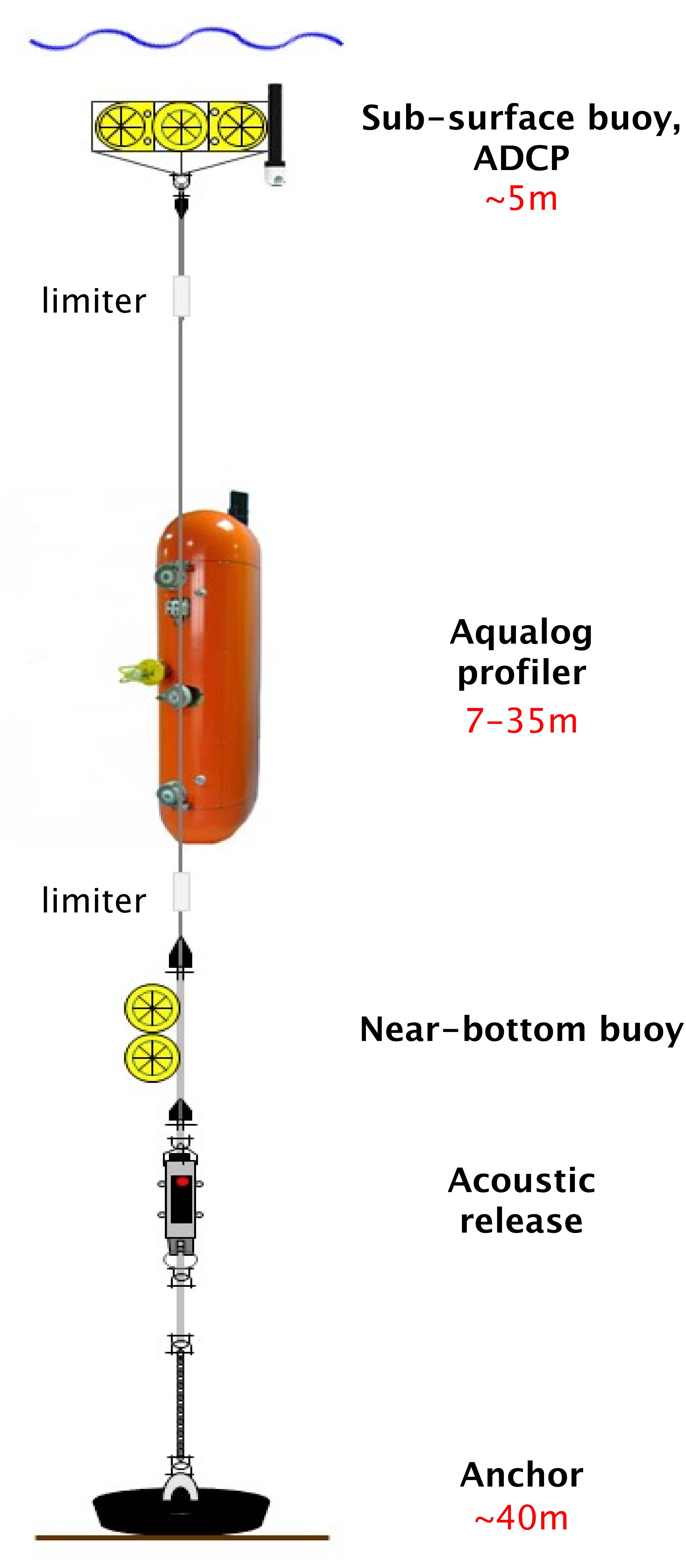
Figure 2. Design of the profiling system.

TABLE 1

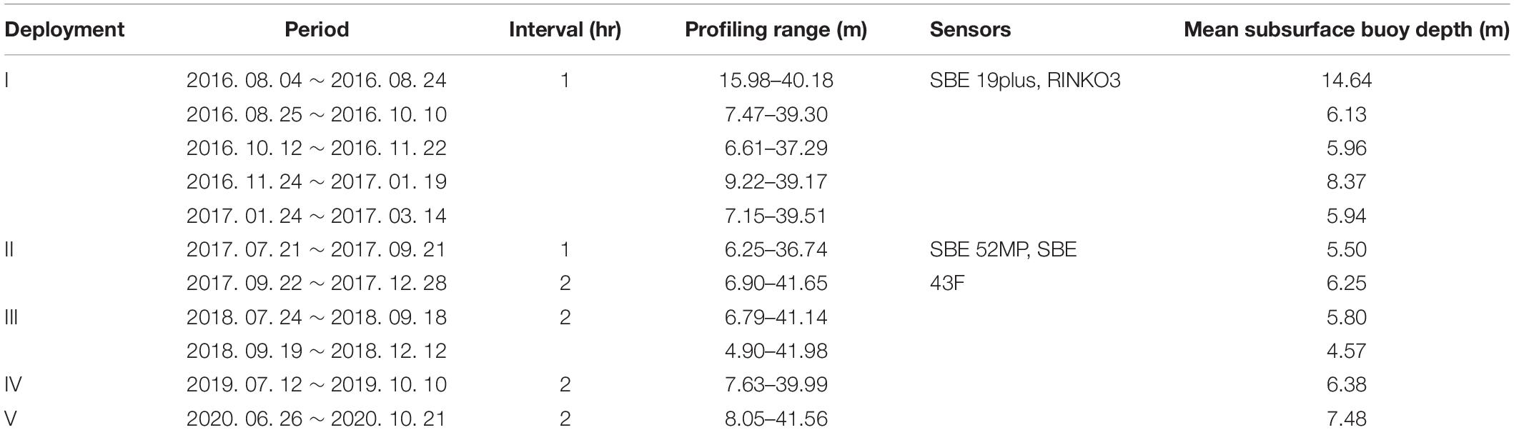
Table 1. Summary of deployments.

From August 2016 to October 2020, there were five deployments. During Deployment I, which lasted for about 7 months, there were five Segments and four maintenances during which the battery and mooring line were replaced and the carrier was cleaned. During Deployments II and III, there were two segments and one maintenance. From Deployments I through III, it was found that during winter and spring the water was relatively homogeneous, and Deployments IV and V were conducted only during summer without any maintenance, while increasing the sampling interval from one to 2 h. Since this area has been used as a test bed, once in a while the mooring system became entangled with other instrument and the profiling system did not work properly. After Deployment IV, we found that the shaft and pulley of the motor in the carrier were corroded and replaced them. To collaborate or coordinate with other mooring systems deployed into the area, the profiling system was not always kept the same location, as depicted in Figure 1.

Biofouling and Cleaning

Since this coastal area is highly productive, biofouling was a major concern. In Figure 3, the conditions of the subsurface buoy and the profiler after 2-month-long deployment are shown. The subsurface buoy that was placed about 5 meters below the surface was contaminated more than the profiler. The line was clean because the profiler moved regularly. The inside of the profiler was also contaminated. These organisms were removed on site by water jets, and if necessary the system was moored again. Even though the profiler was parked 5 m above the bottom, there were sediments inside the carrier due to the tidal currents. As explained later biofouling, however, did not degrade the CTD data, at least for our coastal applications.

FIGURE 3

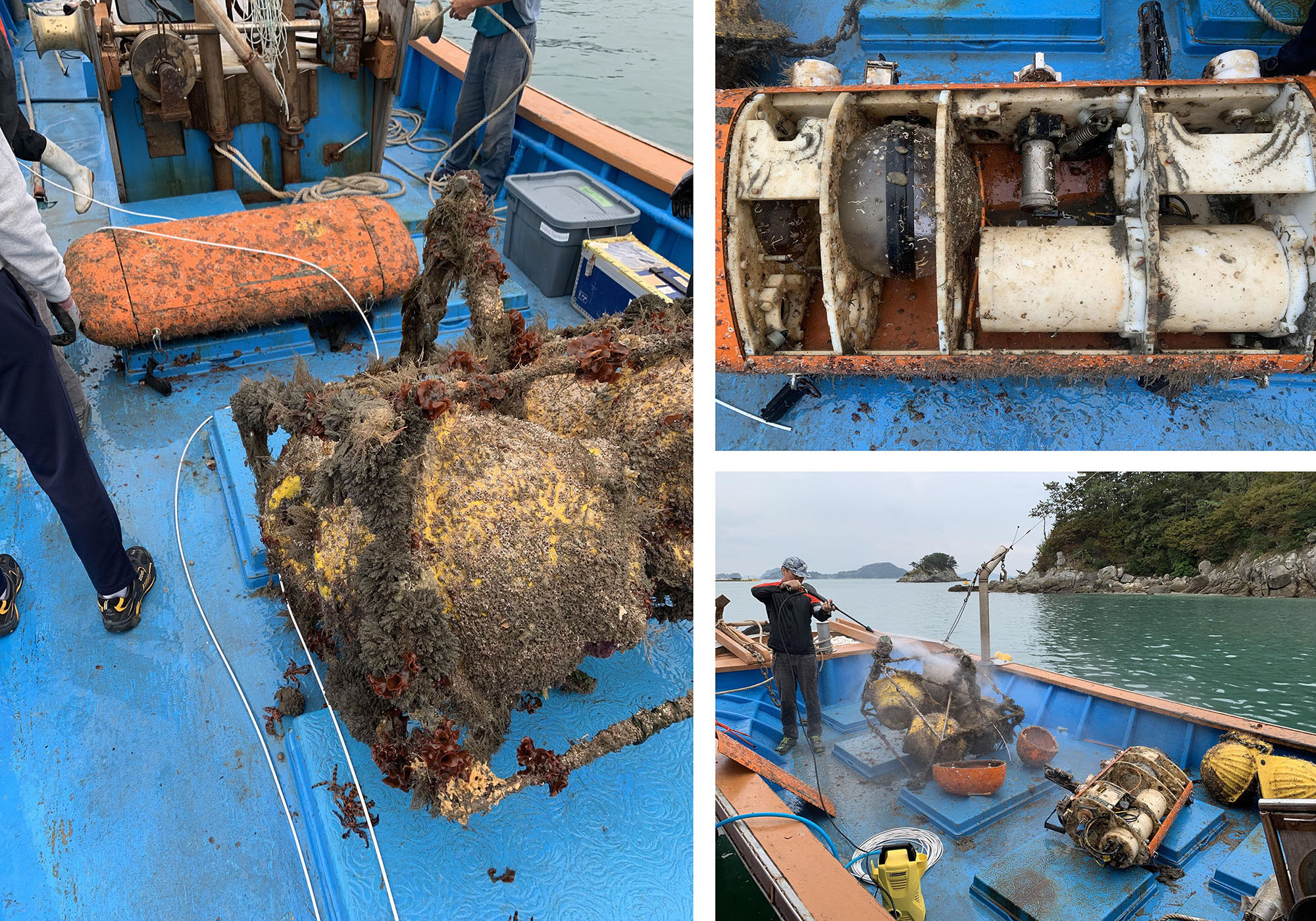
Figure 3. Biofouling and cleaning.

Results

In Figure 4, the data collected during Deployment I are displayed. The prominent signals are tide and coastal warm/fresh water events as explained more in detail later. Since mid-September the amount of the fresh water from the Yangtze River decreased, and the salinity was increased. The area had been hit by typhoons a few times and the responses of the water to the typhoons were also recorded. From November 1 to late November, there was not enough battery power, and the profiler stopped. We miscalculated the remaining battery life, and did not replace the battery pack during the maintenance. During Segment 1, due to security concern the subsurface buoy was placed rather deep and the profile stopped at 15 m below the surface. During the first maintenance, the subsurface buoy was raised to about 5 m and the profile was obtained up to about 8 m.

FIGURE 4

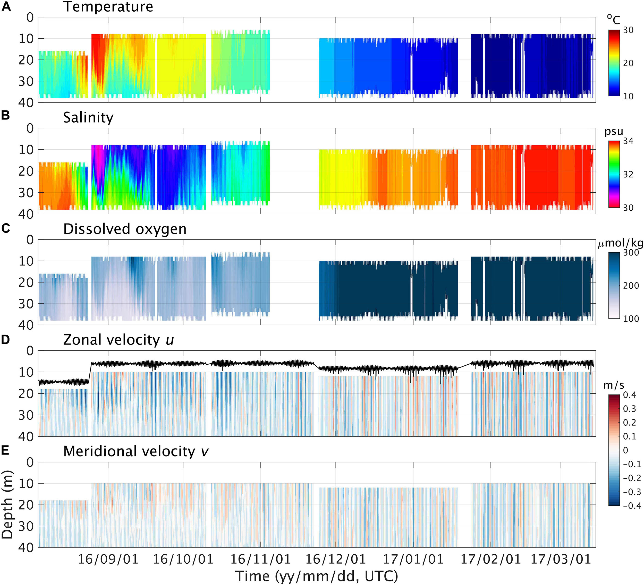
Figure 4. Data from the profiling system (A) temperature, (B) salinity, (C) dissolved oxygen, and (D) zonal, u, and (E) meridional velocity, v, from the Aquadopp installed to the subsurface buoy. The solid line in (D) is pressure from the Aquadopp and shows the depth of the subsurface buoy.

Under a strong flow, the mooring line could be drooped so that the profiler may not be able to move properly. Between August 4, 2016 and March 11, 2017 there were five of such events. Using pressure data from the ADCP installed at the subsurface buoy, the angle between the mooring line and the vertical line was estimated during those events (Figure 5). It was found that when the angle was less than about 22 degrees or the ambient current was 0.6 m/s, the profiler worked properly. If the angel was less than 20 degrees, the profiler worked properly even at higher speed, as suggested by the manufacturer. Even after the mooring line became vertical, it took several cycles for the profiler to function properly probably again due to the misalignment between the rollers and the mooring line. Since the surface current is stronger it is more likely to have this problem as the subsurface buoy was raised.

FIGURE 5

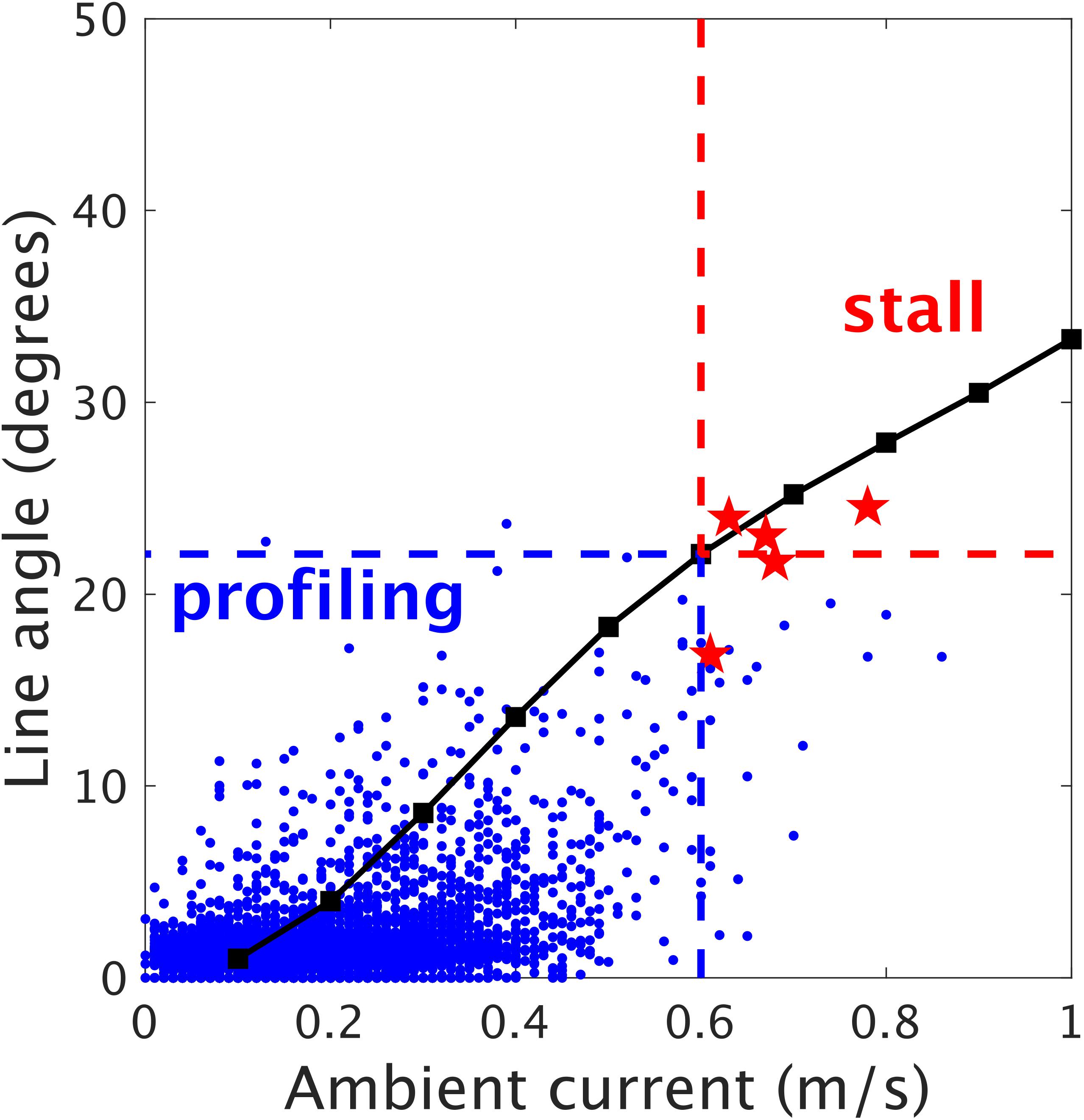
Figure 5. Range for profiling.

Validation of Data

Since the instruments were deployed more than 6 months, the quality of the data must be verified first. Temperature and salinity were verified by comparing with the hydrographic observations made just before the deployments of the mooring system in Figure 6. Temperature showed an offset of about 0.02 but not a drift. Salinity, however, was reduced by approximately 0.01 psu/month. This is highly productive costal area and we were expecting rather rapid contamination but it was less than what we expected. The profiler was parked below euphotic zone and must therefore be contaminated less than expected. The drift was rather linear and could be corrected using the hydrographic data. This amount of drift would be substantial for an open ocean and must be corrected (Ando et al., 2005), but in this coastal area it was much smaller compared to the daily or seasonal changes in salinity and the correction was not made. Instead we calibrate the sensor once a year, typically.

FIGURE 6

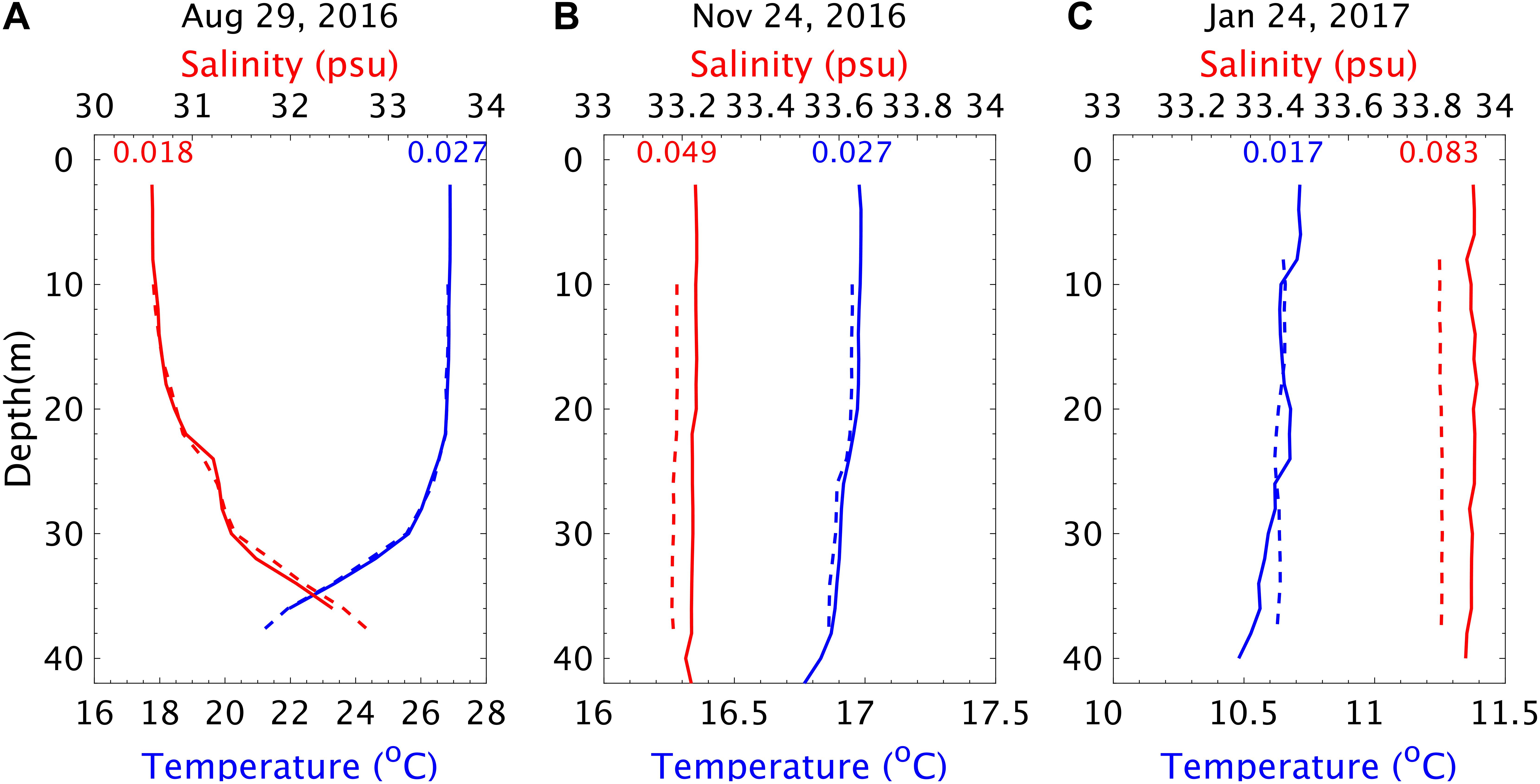
Figure 6. Comparisons of temperature and salinity from the profiler and hydrographic data on three different days on (A) August 29, 2016, which is 25 days, (B) November 24, 2016, 112 days, and (C) January 24, 2017, 173 days after the first deployment. The dashed line is for the profiler and the solid one for the hydrographic observations. The numbers in the figure represent the difference between the two within upper mixed layer in each case. The time difference between the profiler and the hydrographic cast is less than 1.5 h in all three.

Using another CTD, SBE19plus equipped with SBE43F dissolved oxygen, daily hydrographic casts were also conducted at the research station from August 26, 2016 to September 9, and compared with DO from the profiler as shown in Figure 7. In general, the two data sets are consistent. DO data from other period is within a comparable range except for winters when air-sea interaction was active, and we can conclude that the DO sensor installed to the profiler was not contaminated seriously. One interesting feature from the data is that temperature and DO are positively correlated. At the particular site a warm water event is not causing hypoxia on the contrary to common belief. The cause and the structure of the warm water will be reported in a separate paper.

FIGURE 7

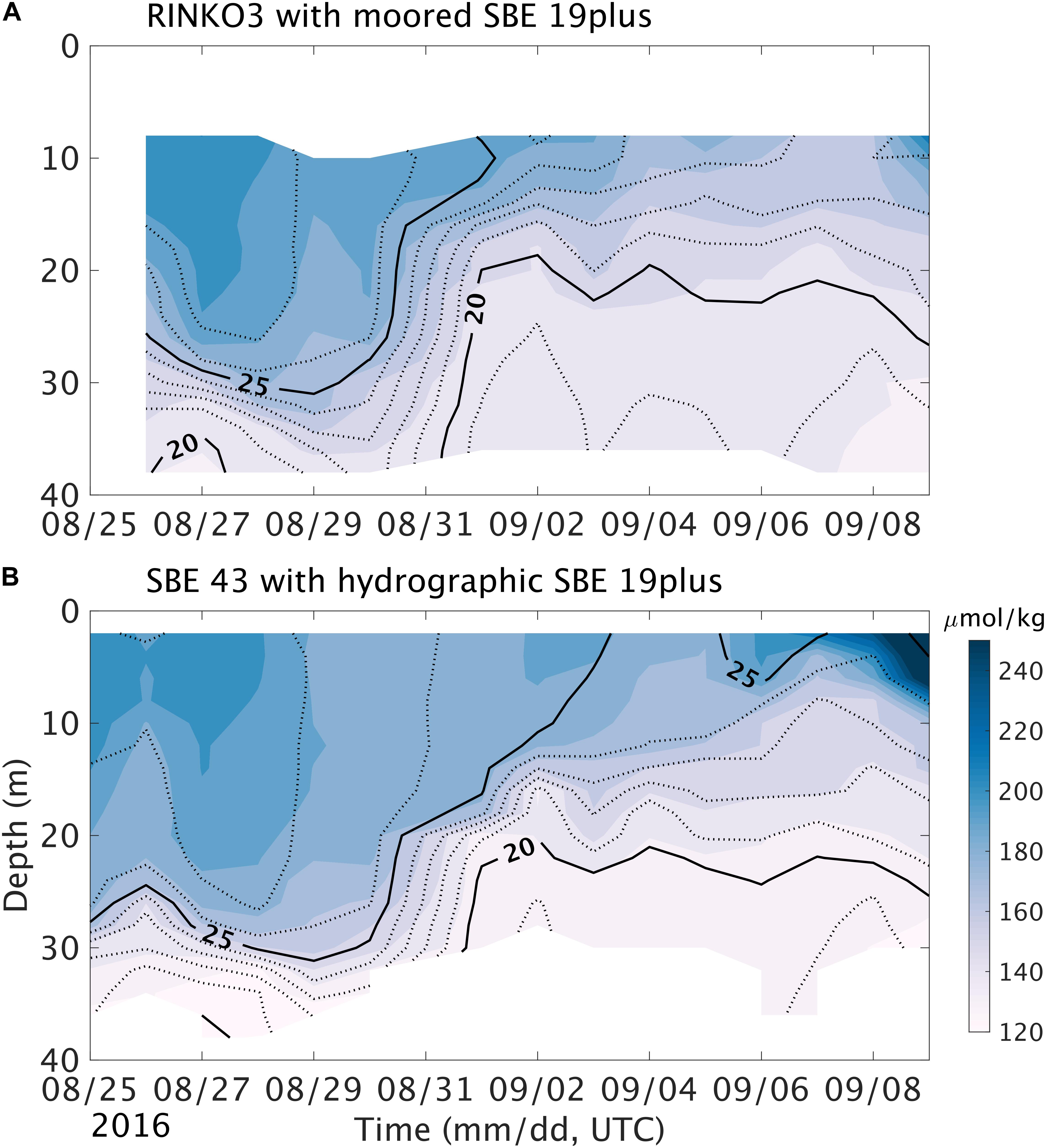
Figure 7. Dissolved oxygen (shading) and temperature (contours) from (A) the profiler and (B) daily hydrographic casts made at the research station. The time difference between the two data set is less than an hour.

The site is close to a pier and easily accessible, but at the same is too close to the coast so that the data may just show local properties. There is no river around the site that is located over the headland. Thus it is rather unlikely that our data just show local structure. To verify our assumption, in Figure 8 the data from the profiler shown in Figure 4 are compared with hydrographic data taken by the Korea Oceanographic Data Center (KODC, 2017) at stations shown in Figure 1, 206-00, 206-01 and 206-02 which are 15, 26, and 41 km away from the mooring site, respectively. Except for the relatively salty (>34 psu) affected by Tsushima Warm Current water (Hyun et al., 1996; Pang et al., 1996) found further offshore, the profiler captured the warm and fresh upper and subsurface water found in the southern part of the Korea. The cold and salty winter coastal water was also well observed during Segment 5 (green dots).

FIGURE 8

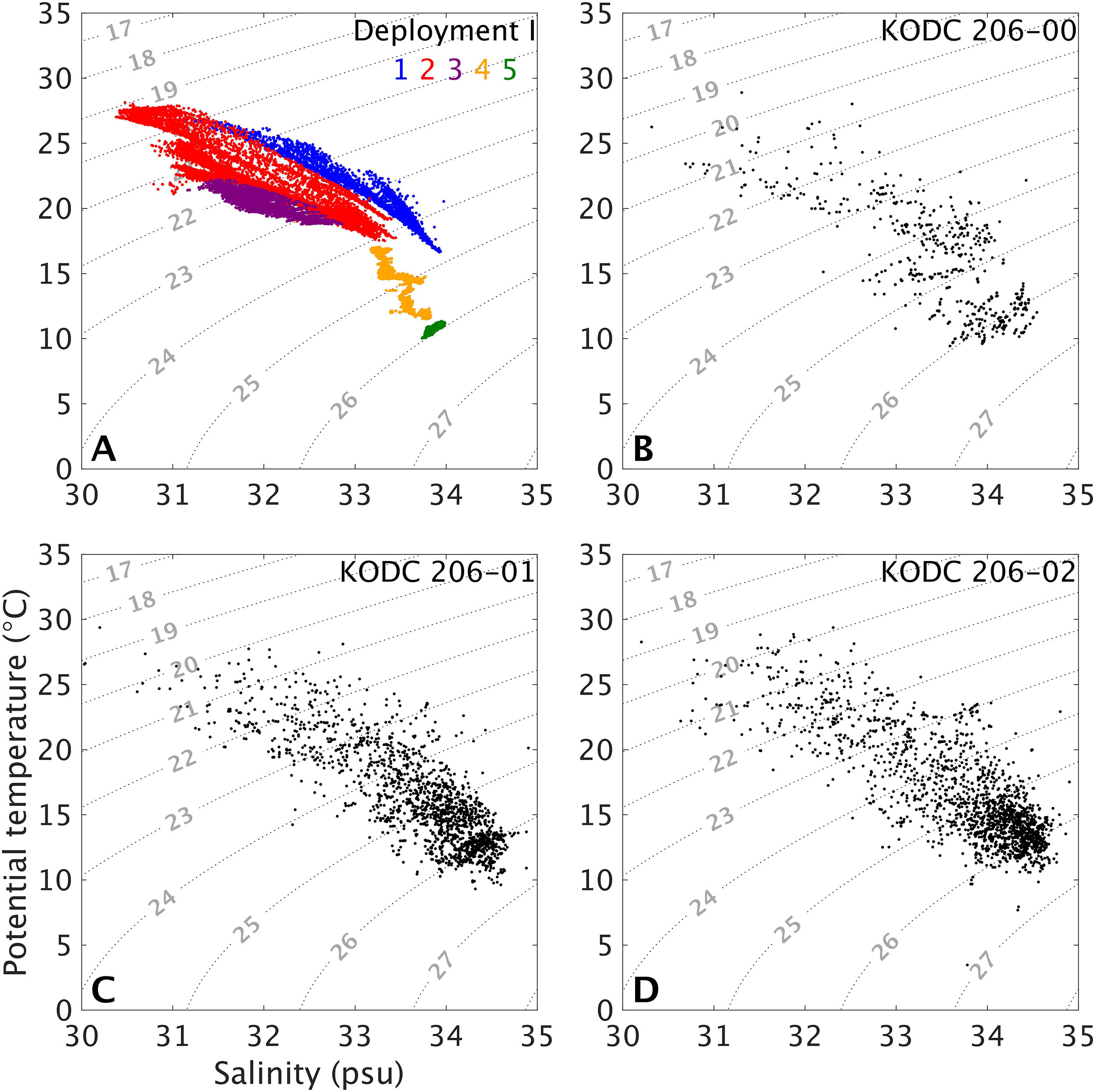
Figure 8. T-S diagrams using data (A) from Deployment I, and hydrographic data from (B) KODC 206-00, (C) KODC 206-01, and (D) KODC 206-02 sites shown in Figure 1. The different colors in (A) represent different segments during Deployment I.

Tide

As in other southern Korean coastal areas (Teague et al., 2001) the most dominant signal from the current is M₂, followed by S₂ and then K₁, as well as from the pressure obtained at the subsurface buoy. In Figure 9, the tide during August 2016 when the water was well stratified and that in December 2016 when the water was well mixed, are shown. During August, the tidal current was strongly baroclinic while during December barotropic. Seasonality in barotropic tide is known (Kang et al., 1995), but such a change in vertical structure has not been reported previously. In this area, due to the strong stratification, the Richardson Number is >0.25, and the velocity shear would not be able to induce vertical mixing. Whether the baroclinicity is limited to this coastal area or common to other parts is a topic for future studies.

FIGURE 9

Figure 9. Temperature (A,B), salinity (C,D), zonal velocity u (E,F), and meridional velocity v (G,H) during summer (left column) and winter (right column).

Warm Water Event

Warm water events were observed every summer. Explaining the structure of this warm water itself is beyond the scope of this study and here we want describe the basic structure and the benefits of using continuous measurement. The shortest time scale of the warm water event is due to the diurnal tide (Figure 9). The warm water is not produced locally but remotely. During the flood tide warm and fresh water flows from northwest and fills the area so that the amount of the warm and fresh water becomes greatest during high tide. During the ebb the warm and fresh water retreats. The warm water also shows variations between 10 and 15 days due to onshore advection (Figure 10). The dynamics behind the onshore advection is yet to be studied. One may conclude that this time scale is tied to the spring-neap cycle, but close investigation using all the data shows that they are not correlated. Since this warm water event is due to freshwater from the Yangtze River (Park et al., 2011; Kako et al., 2016; Moon et al., 2019), temperature and salinity are negatively correlated. In Korea, there are surface buoys measuring surface temperature, but the vertical extent of the warm water cannot be estimated with such data. This large change in the vertical extent would be useful information to local aquafarms. In open ocean, there is no data showing temporal variation and we used model outputs. Warm water events are rather continuous and do not show the variation observed with the profiler, suggesting that the temporal structure is limited to this coastal area. If this applies to other coastal area, more specific warning system taking into account vertical extent and duration is required. Around Korea, hydrographic observations have been made every 2 months. These data are useful in studying the long term changes and the mean state, but naturally cannot resolve the warm water events.

FIGURE 10

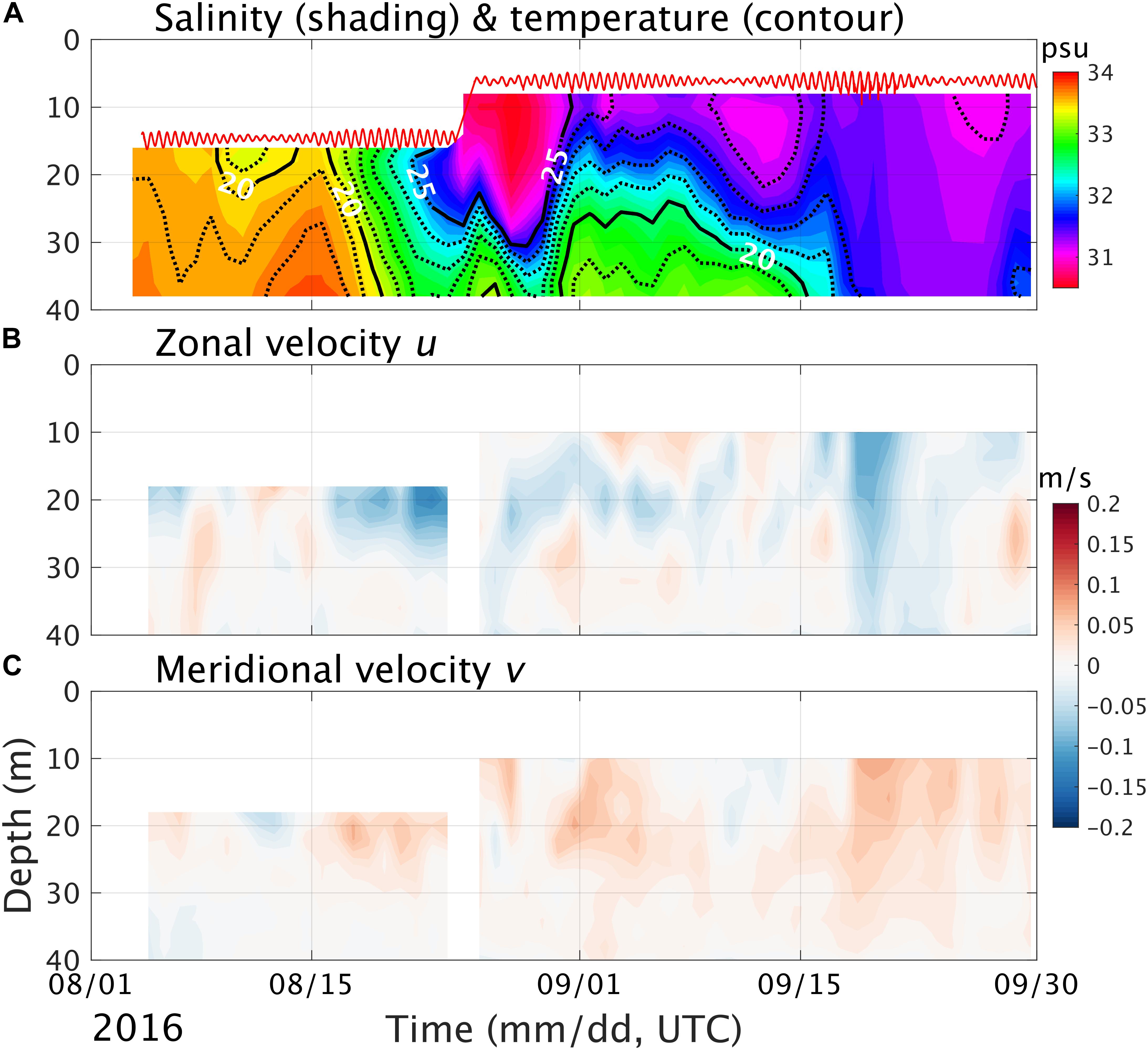
Figure 10. Warm water events in summer 2016. Daily mean (A) salinity (shading) and temperature (contour), (B) zonal velocity, u, and (C) meridional velocity, v.

Response to Typhoons

During the deployment, six typhoons passed by the observation site as displayed in Figure 11, and the data provide us with a rare opportunity to investigate the response of the coastal water to typhoons. In open oceans, a typhoon enhances vertical mixing to mix warm surface water with the cooler subsurface layer, causing a deeper mixed layer and cold wake at the surface (Price, 1981). In coastal waters, due to topography and lateral boundaries, the response could be different from that in open ocean.

FIGURE 11

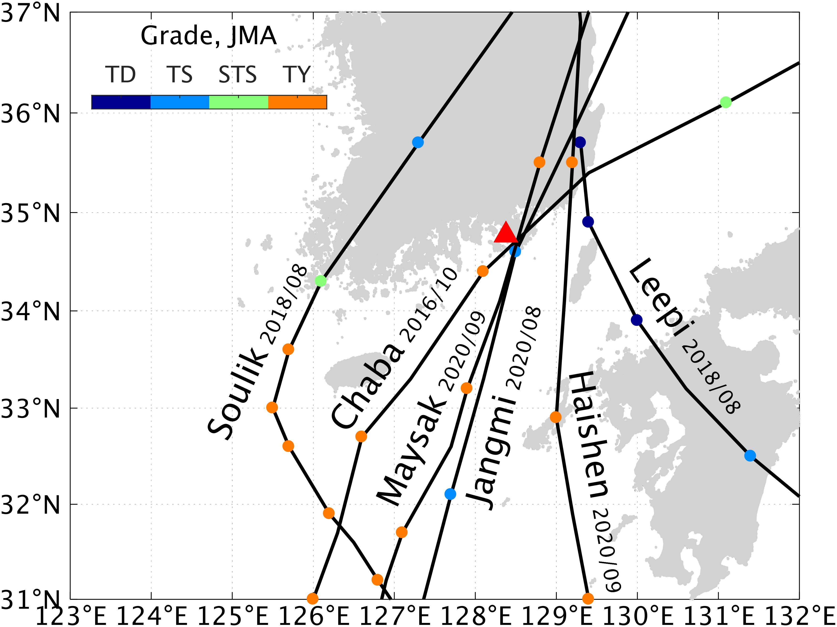
Figure 11. Tracks of the typhoons passed by the observation site (red triangle) at 6-h intervals. The color bar in the upper left corner represents the typhoon category. Tropical Depression (TD), Tropical Storm (TS), Severe Tropical Storm (STS), Typhoon (TY).

During Typhoons Chaba in 2016 and Maisak and Haisen in 2020, the mooring site was hit by winds of about 20 m/s or stronger. Since the mooring was under the water, it produced nice data without any damage. In the case of Chaba 2016, as the wind became stronger salty and cold water was advected toward the observation site, the stratification between 20∼30 m levels became stronger (Figure 12). This tendency continued until 10 h after the wind speed reached the maximum, after which mixed water started to appear. This observation suggests that the effect of advection was stronger than local mixing. During Typhoon Maysak on September 1st 2020, as the wind intensified, the mixed layer became deeper. Note that since we are lacking data for the upper 10 m, the mixed layer depth cannot be defined strictly. Instead, the 24°C isotherm was used as a proxy for the mixed layer depth. The mixed layer became deepest when the wind was strongest (Figure 13). It was possible to reproduce this deepening tendency using a 1-D mixed layer model such as GTOM (Burchard, 1999, available at¹). In a mixed layer model, the initial upper layer stratification governs the subsequent evolution of temperature. In this case, the upper layer structure is unknown, and by assuming a rather strong stratification within upper 10 m, it was possible to reproduce the deepening of the 24°C isotherm (not shown). The mixed layer disappeared within less than a day due to subsurface advection of cold and salty water from south. The 1-D mixed layer model was not able to reproduce the disappearance of the mixed layer, however. The global analysis field from the HYbrid Coordinate Ocean Model (HYCOM, GOFS 3.1²) whose horizontal resolution is 1/12° was able to reproduce the deepening of the mixed layer due to the typhoon. The disappearance of the mixed layer was not reproduced probably because the horizontal resolution is not high enough to resolve the coastal circulation properly. During Typhoon Haisen, which arrived about 4 days after Typhoon Maysak, the water column does not show notable response to the increasing wind until a few hours before the peak wind (Figure 14). Then, the mixed layer started to thicken rather slowly and became thickest about 12 h after the peak wind. The thick mixed layer was maintained for a few days. Tidal currents were strong but the two typhoons homogenized water around the observation site and the water remain homogeneous.

FIGURE 12

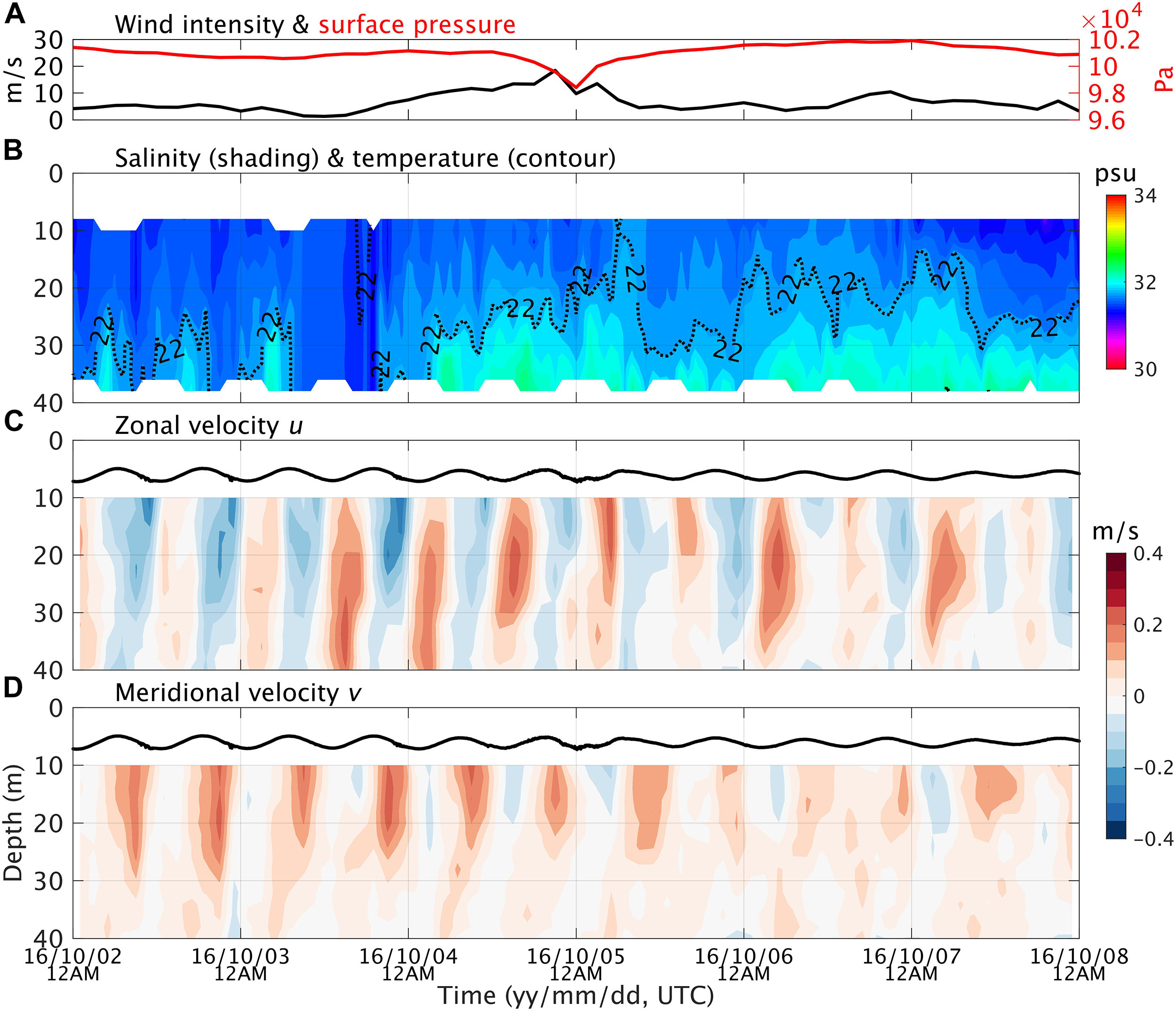
Figure 12. Responses to Typhoon Chaba. (A) wind strength (back line) and surface pressure (red line) from European Centre for Medium-Range Weather Forecasts (ECMWF) ERA5 (Hersbach et al., 2020), (B) salinity (shading) and temperature (contour), (C) zonal velocity, u, and (D) meridional velocity, v.

FIGURE 13

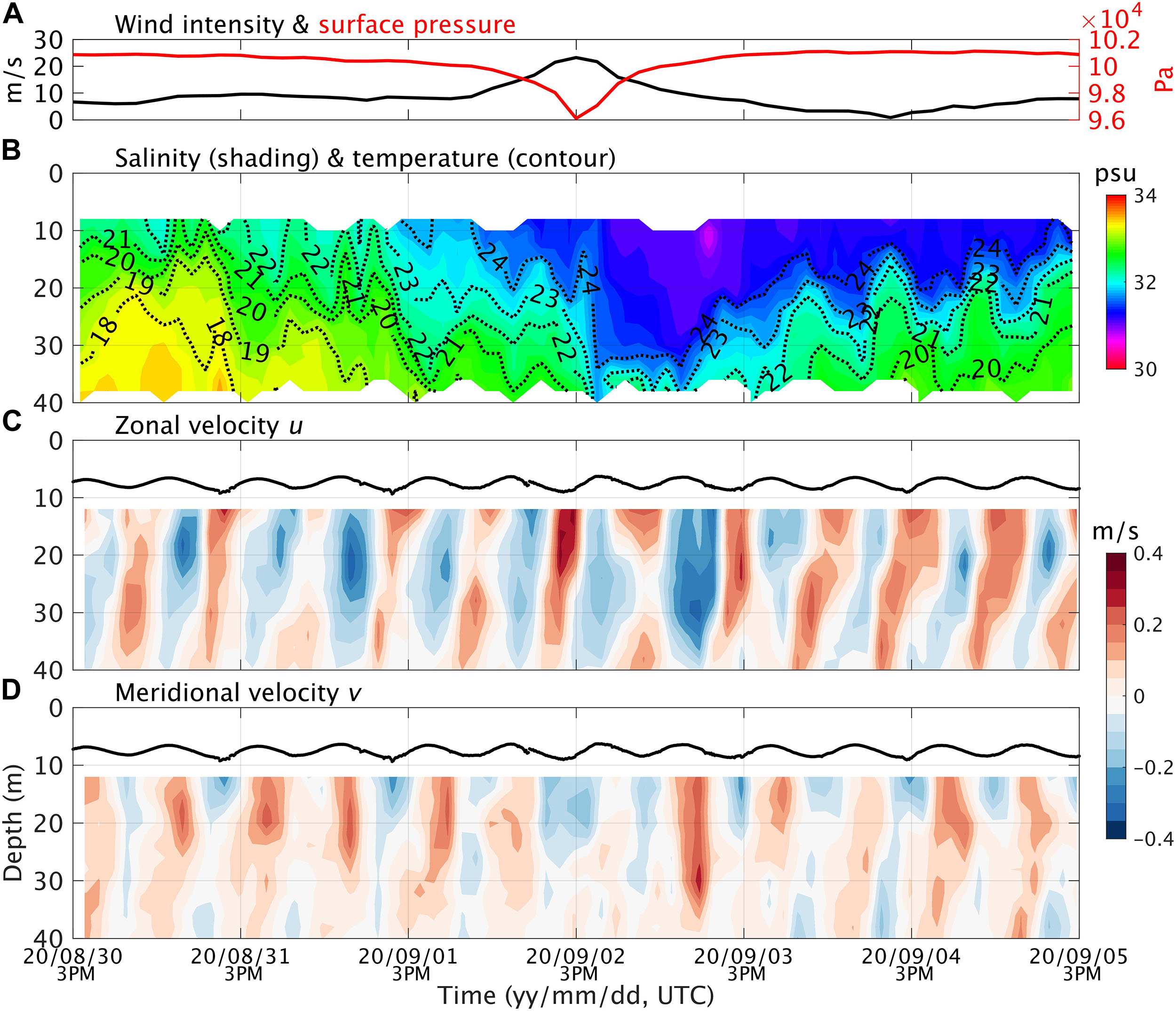
Figure 13. The same as Figure 12 except for Typhoon Maysak.

FIGURE 14

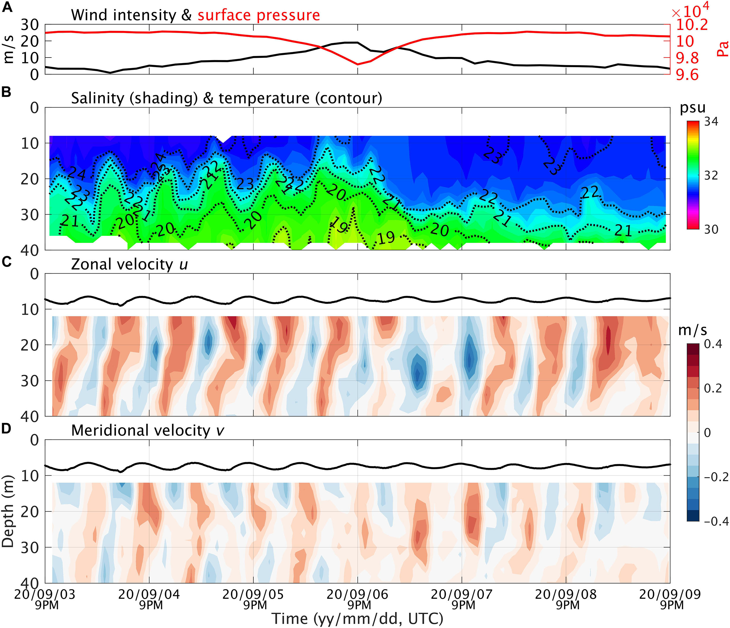
Figure 14. The same as Figure 12 except for Typhoon Haishen.

Summaries and Conclusion

At a coastal research station located at the southern coastal area of Korea, a vertical profiling system measuring temperature, salinity, dissolved oxygen, and velocity has been successfully maintained every summer from 2016 to 2020. Around the station, fishing activity is not allowed, and it has thus been possible to maintain the profiler continuously and stably. Comparisons with hydrographic data show that the sensors were contaminated much less than we expected during 2- to 6-month-long deployments probably because the sensors were located below the euphotic zone. Therefore, the data could be used without correction for our coastal applications. Even though the station is within 2 km of the land, there is no river and the profiler observed the warm and fresh southern coastal water of Korea well. When the profiler did not operate properly, this was because the flow was stronger than about 0.6 m/s so that mooring line was inclined from the vertical by more than 20 degrees.

The profiling system recorded continuous spatiotemporal variations that cannot be measured using hydrographic surveys or point measurements at a surface buoy. The semi-diurnal tides were the most prominent phenomenon, as in other coastal areas around Korea. It was found for the first time that in summer, when the water is strongly stratified, the tidal current is baroclinic, while in winter, when the water is well mixed, the current is barotropic. The baroclinicity was not strong enough to overcome the stratification sufficiently to induce vertical mixing, however. The strong seasonality calls for a further study on the dynamics and its effect on coastal environments. Coastal warm water events were also prominent. On the daily time scale, the semi-diurnal tide was the main driver. During the flood, warm and fresh water was transported from the offshore while during the ebb retreated to the offshore. The warm water also showed fluctuations between 10 and 15 days due to northward advection from the offshore. Numerical model results show that such variations do not occur in offshore waters. The profiling system deployed underwater recorded the responses to typhoon-induced winds without any damage. Both lateral advection and wind-induced vertical mixing were important.

The collected time series can be used in verifying coastal ocean circulation models as well as for data assimilation once real-time data become available. There are diverse types of aquafarms in the study area, and the data help the stake holders in selecting the optimal site for such farms as demonstrated in Chang et al. (2020). Coastal warm water events are becoming serious concerns to aquafarms. The variability and characteristics of the warm water events we reported would be of much help in establishing effective countermeasures.

The main limitation with the profiling system is real-time communication, and the data have not been used for real-time prediction so far. Another limitation is the lack of surface data. The upper most temperature from the profiler was lower by 5 to 2°C than surface temperature obtained from a nearby surface buoy. To overcome these deficiencies, we plan to upgrade the profiling system using a surface buoy equipped with a temperature sensor and a real-time communication system utilizing an acoustic modem and a cellular modem.

Data Availability Statement

The raw data supporting the conclusions of this article will be made available by the authors, without undue reservation.

Author Contributions

Y-GP led the project, interpreted the data, and wrote the manuscript. SS performed data analysis and visualization. DK contributed to the design of the mooring, data acquisition, and processing. DK, SS, JN, and HP contributed to the maintenance of the mooring system and instruments, data acquisition, and processing. All authors contributed to manuscript revision, and approved the submitted version.

Funding

This work was funded through the projects “Investigation and prediction system development of marine heatwave around the Korean Peninsula originated from the subarctic and western Pacific (20190344)” from the Ministry of Oceans and Fisheries, Korea, and “Building Conceptual Design for Mid-size Integrated CCS Demonstration (20214710100060)” from the Korea Institute of Energy Technology Evaluation and Planning.

Conflict of Interest

The authors declare that the research was conducted in the absence of any commercial or financial relationships that could be construed as a potential conflict of interest.

Acknowledgments

We would like to thank Yong-Joo Park and the members of Tongyoung Marine Living Resources Station for their support.

Footnotes

1. ^ www.gotm.net
2. ^ https://www.hycom.org

References

Ando, K., Matsumoto, T., Nagahama, T., Ueki, I., Takatsuki, Y., and Kuroda, Y. (2005). Drift characteristics of a moored conductivity-temperature-depth sensor and correction of salinity data. J. Atmos. Ocean Technol. 22, 282–291. doi: 10.1175/jtech1704.1

CrossRef Full Text | Google Scholar

Burchard, H. (1999). Recalculation of surface slopes as forcing for numerical water column models of tidal flow. Appl. Math. Model. 23, 737–755. doi: 10.1016/s0307-904x(99)00008-6

CrossRef Full Text | Google Scholar

Carlson, D. F., Ostrovskii, A., Kebkal, K., and Gildor, H. (2013). “Moored automatic mobile profilers and their applications,” in Advances in Marine Robotics, ed. G. Oren (Riga: LAP Lambert Academic Publishing), 169–206.

Google Scholar

Chang, Y. S., Jin, J., Choi, J. Y., Jeong, W. M., Hyun, S. K., Chung, C. S., et al. (2020). Three dimensional numerical modeling using a multi-level nesting system for identifying a Water layer suitable for scallop farming in Tongyeong, Korea. Aquac. Eng. 89:102058. doi: 10.1016/j.aquaeng.2020.102058

CrossRef Full Text | Google Scholar

Dunne, J. P., Devol, A. H., and Emerson, S. (2002). The oceanic remote chemical/optical analyzer (ORCA)—an autonomous moored profiler. J. Atmos. Ocean Technol. 19, 1709–1721. doi: 10.1175/1520-0426(2002)019<1709:torcoa>2.0.co;2

CrossRef Full Text | Google Scholar

Fayman, P., Ostrovskii, A., Lobanov, V., Park, J. H., Park, Y. G., and Sergeev, A. (2019). Submesoscale eddies in Peter the Great Bay of the Japan/East Sea in winter. Ocean Dyn. 69, 443–462. doi: 10.1007/s10236-019-01252-8

CrossRef Full Text | Google Scholar

Forrester, N., Stokey, R. P., Von Alt, C., Allen, B. G., Goldsborough, R. G., Purcell, M. J., et al. (1997). “The LEO-15 long-term ecosystem observatory: design and installation,” in Proceedings of the Oceans ‘97 Conference MTS/IEEE, Halifax, NS.

Google Scholar

Hersbach, H., Bell, B., Berrisford, P., Hirahara, S., Horányi, A., Muñoz-Sabater, J., et al. (2020). The ERA5 global reanalysis. Q. J. R. Meteorol. Soc. 146, 1999–2049.

Google Scholar

Hyun, K. H., Pang, I. C., and Rho, H. K. (1996). The seasonal circulation in the South and West Seas and the inflow of warm waters into the West Sea in summer. Bull. Mar. Res. Inst. Cheju Nat. Univ. 20, 17–30.

Google Scholar

Kako, S. I., Nakagawa, T., Takayama, K., Hirose, N., and Isobe, A. (2016). Impact of Changjiang River discharge on sea surface temperature in the East China Sea. J. Phys. Oceanog. 46, 1735–1750. doi: 10.1175/jpo-d-15-0167.1

CrossRef Full Text | Google Scholar

Kang, S. K., Chung, J. Y., Lee, S. R., and Yum, K. D. (1995). Seasonal variability of the M2 tide in the seas adjacent to Korea. Cont. Shelf Res. 15, 1087–1113. doi: 10.1016/0278-4343(94)00066-v

CrossRef Full Text | Google Scholar

KODC (2017). Korea Oceanographic Data Center. Available online at: http://kodc.nfrdi.re.kr (accessed April 1, 2017).

Google Scholar

Kolding, M. S., and Sagstad, B. (2013). Cable-free automatic profiling buoy. Sea Technol. 54, 10–12.

Google Scholar

Moon, J. H., Kim, T., Son, Y. B., Hong, J. S., Lee, J. H., Chang, P. H., et al. (2019). Contribution of low-salinity water to sea surface warming of the East China Sea in the summer of 2016. Prog. Oceanogr. 175, 68–80. doi: 10.1016/j.pocean.2019.03.012

CrossRef Full Text | Google Scholar

Ostrovskii, A. G., and Zatsepin, A. G. (2011). Short-term hydrophysical and biological variability over the northeastern Black Sea continental slope as inferred from multiparametric tethered profiler surveys. Ocean Dyn. 61, 797–806. doi: 10.1007/s10236-011-0400-0

CrossRef Full Text | Google Scholar

Ostrovskii, A. G., Zatsepin, A. G., Shvoev, D. A., and Soloviev, V. A. (2010). “Underwater anchored profiler Aqualog for ocean environmental monitoring,” in Advances in Environmental Research, ed. J. A. Daniels (New York, NY: Nova Science Publishers, Inc), 179–196.

Google Scholar

Ostrovskii, A. G., Zatsepin, A. G., Soloviev, V. A., Tsibulsky, A. L., and Shvoev, D. A. (2013). Autonomous system for vertical profiling of the marine environment at a moored station. Oceanology 53, 233–242. doi: 10.1134/s0001437013020124

CrossRef Full Text | Google Scholar

Pang, I. C., Rho, H. K., Lee, J. H., and Lie, H. J. (1996). Water mass distribution and seasonal circulation northwest of Cheju Island in 1994. Korean J. Fish. Aquat. Sci. 29, 862–875.

Google Scholar

Park, T., Jang, C. J., Jungclaus, J. H., Haak, H., and Park, W. (2011). Effects of the Changjiang river discharge on sea surface warming in the Yellow and East China Seas in summer. Cont. Shelf Res. 31, 15–22. doi: 10.1016/j.csr.2010.10.012

CrossRef Full Text | Google Scholar

Price, J. F. (1981). Upper ocean response to a hurricane. J. Phys. Oceanogr. 11, 153–175. doi: 10.1175/1520-0485(1981)011<0153:uortah>2.0.co;2

CrossRef Full Text | Google Scholar

Rixen, M., Book, J. W., and Orlic, M. (2009). Coastal processes: challenges for monitoring and prediction. J. Mar. Syst. 78, S1–S2.

Google Scholar

Teague, W. J., Perkins, H. T., Jacobs, J. W., and Book, J. W. (2001). Tide observation in the Korea-Tsushima Strait. Cont. Shelf Res. 21, 545–561. doi: 10.1016/s0278-4343(00)00110-2

CrossRef Full Text | Google Scholar

Von Alt, C., De Luca, M. P., Glenn, S. M., Grassle, J. F., and Haidvogel, D. B. (1997). LEO-15: monitoring and managing coastal resources. Sea Technol. 38, 10–16.

Google Scholar

Weller, R. A., Baker, D. J., Glackin, M. M., Roberts, S. J., Schmitt, R. W., Twigg, E. S., et al. (2019). The challenge of sustaining ocean observations. Front. Mar. Sci. 6:105. doi: 10.3389/fmars.2019.00105

CrossRef Full Text | Google Scholar