 Sonia Sánchez-Maroño
 Andrés Uriarte
 Leire Ibaibarriaga
 Leire Citores
- Marine Research, AZTI, Basque Research and Technology Alliance (BRTA), Pasaia, Spain
Most of the methods developed for managing data-limited stocks have been designed for long-lived species and result in a poor performance when applied to short-lived fish due to their high interannual variability of stock size (IAV). We evaluate the performance of several catch rules in managing two typical short-lived fish (anchovy-like: characterized by high natural mortality, and hence, IAV, and full maturity at age 1; and sprat/sardine-like: with medium natural mortality and IAV, being fully mature at age 2). We followed the management strategy evaluation approach implemented in FLBEIA software to test several model-free harvest control rules, where the Total Allowable Catch (TAC) is yearly modified according to the recent trends in an abundance index (n-over-m rules: means of the most recent n values over the precedent m ones). The performance of these rules was assessed across a range of settings, such as time-lags between the index availability and management implementation, and alternative restrictions on TACs’ interannual variability (the uncertainty caps, UC). Moreover, we evaluated the sensitivity of the rule performance to the operating model assumptions (stock type, productivity, recruitment variability and initial depletion level) and to the observation error of the index. In general, the shorter the lag between observations, advice and management, the bigger the catches and the smaller the biological risks. For in-year management, 1-over-m rules are reactive enough to stock fluctuations as to gradually reduce risks. The 1-over-2 rule with symmetric 80% UCs reduces catches and risks toward precautionary levels in about 10 years, faster than if applied unconstrained (i.e., without UC), whilst the ICES default 2-over-3 rule with symmetric 20% UC is not precautionary. We prove that unconstrained rules gradually reduce the fishing opportunities, with amplified effects with increasing IAV. This property explains the stronger reductions of catches and risks achieved for the anchovy compared to the sprat/sardine-like stocks for any rule and the balance between catches and risks as the index CV increases. However, to avoid unnecessary long-term losses of catches from such reduction properties, it is suggested that the rules should be applied provisionally until a better assessment and management system is set up.
Introduction
The majority of the stocks exploited worldwide are from fisheries that lack formal stock assessments (Beddington et al., 2007; Costello et al., 2012; Ricard et al., 2012). These are usually low value resources (Bentley and Stokes, 2009b), often corresponding to by-catch, small-scale, recreational and/or artisanal fisheries. But there are also cases in which the quality of the data hinders its use for assessment purposes or there is insufficient capacity to conduct stock assessments (Dowling et al., 2019). In an attempt to decrease the number of stocks with unassessed status and to provide management advice for the largest number of species as possible, several jurisdictions have developed hierarchical tier systems that categorize stocks based on the data available or the ability to estimate key assessment parameters (Dichmont et al., 2015). Aiming at reducing risks to sustainability, but still maintaining profitable fleets and addressing food security issues (United Nations, 2019).
The International Council for the Exploration of the Sea (ICES), that provides management advice for many European fisheries, started to develop its tier system, the so-called data-limited framework, in 2012 (ICES, 2012a). Since then, this framework has evolved over time through several expert working groups that have validated and refined many of the methods proposed (ICES, 2012b, 2020c). Nowadays ICES classifies stocks into six categories based on the available information (ICES, 2019). Category 1 comprises stocks with full analytical stock assessment and forecasts. Category 2 refers to stocks with analytical assessments and forecasts that are only treated qualitatively as indicative of trends in stock metrics such as recruitment, fishing mortality and biomass. Category 3 includes stocks for which one or more indices (from surveys, from exploratory assessments or from elsewhere) are available and indicative of trends in stock metrics. Categories 4, 5 and 6 are increasingly data-limited stocks for which only catch and/or landing data are available. For each stock, if there is an agreed management plan that has been evaluated to be consistent with the precautionary approach, ICES provides advice based on that plan. Otherwise, ICES provides advice for stocks in categories 1 and 2 based on the ICES maximum sustainable yield (MSY) advice rule that aims at maximizing the average long-term yield while maintaining productive fish stocks, whereas for stocks in categories 3–6 the advice is based on empirical harvest control rules that aim at maintaining the stocks within safe biological limits in accordance with the precautionary approach. In 2014, the majority of the stocks fell in category 3 (ICES, 2014; Dichmont et al., 2015). The empirical harvest control rule used for these stocks adjusts the most recent advised catch according to the ratio of average stock size indices over the last years. In addition, to account for the inherent uncertainty of the index, the interannual change in the catch advice is capped by a maximum change limit called uncertainty cap (UC).
Despite the fact that numerous methods to assess data-limited stocks have been developed in the last years (MacCall, 2009; Dick and MacCall, 2011; Wetzel and Punt, 2011), empirical harvest control rules are emerging as an alternative for data-limited stocks (Bentley and Stokes, 2009a; Dowling et al., 2015). These rules set the management actions based on directly observable indicators rather than from stock assessment models and are readily applicable. Ideally, the performance of these harvest control rules, and more generally the management procedures encompassing them, should be tested by simulation before implementation (Punt et al., 2016). Whenever possible, the simulation testing should be done specifically for each case (Bentley and Stokes, 2009a). However, developing management plans is not trivial, since it demands expertise and can sometimes be resource consuming (Dowling et al., 2019). And it is even more difficult for data-limited stocks, for which information is scarce or less reliable. In these cases, Bentley and Stokes (2009a) argued that generic approaches might not be optimal but can be better than not taking any approach at all. Furthermore, they noted that evaluating generic approaches for a variety of stock characteristics and fishery types could allow to discern which are the most influential factors and gain understanding about concrete circumstances under which the management plans satisfy the objectives.
Generic harvest control rules are usually evaluated for generic stocks (Geromont and Butterworth, 2014; Carruthers et al., 2016) or for specific species (Jardim et al., 2015; Fischer et al., 2020). Often, different species representing contrasting life-traits are selected (Carruthers et al., 2014; Wetzel and Punt, 2015; Walsh et al., 2018). Various simulation studies have shown that the performance of the harvest control rules might change depending on the life history-traits, the productivity of the stock and the depletion level. In particular, in many cases, the performance of the harvest control rules worsened for short-lived fish stocks (those with a lifespan restricted to 4–6 years (ICES, 2017) and becoming fully mature between 1 or 2 years-old). Walsh et al. (2018) showed that choosing an ineffective harvest control rule could have much more dramatic and negative outcomes for short-lived fish species. For Carruthers et al. (2014) butterfish proved to be the most challenging stock due to its short life-span and highly variable recruitment. In a recent paper Fischer et al. (2020) evaluated the performance of the empirical harvest control rule for ICES category 3 stocks for 29 stocks with contrasting life-history parameters. They concluded that the rule performed worse for the more productive stocks (growth parameter of the von Bertalanffy model, k, larger than 0.32 year–1). Stocks with higher k have larger natural mortality (Gislason et al., 2010) and are inherently more variable. This can lead to quick stock recovery, but in this case the rule was not reactive enough to avoid stock collapse.
Some small pelagic fish are good examples of short-lived fish species and of the most common difficulties encountered. Their short life-span, the highly variable recruitment dynamics, the aggregative behaviour of many of them and the quick response to environmental drivers make them vulnerable to exploitation (Freón et al., 2005). The most effective management plans are based on close monitoring with fishery-independent surveys (Barange et al., 2009), short time lag between the stock assessment and the management decision (Freón et al., 2005; Sánchez et al., 2018), pre-recruitment surveys (Dichmont et al., 2006a; Sánchez et al., 2018) or the use of flexible harvest control rules to accommodate the management to the population oscillations, for example setting an initial conservative TAC with a within season adjustment when year-class strength is known (Plagányi et al., 2007).
Representative small pelagics are anchovy, sprat, and sardine. These species are commercially important species and essential in the ecosystem due to their situation in the food-chain, as they are food source for fish, marine mammals, and birds. Maximum anchovy length is around 15–19 cm (corresponding to age of 2 to 5 years) and all individuals are mature at 1 year-old (Barange et al., 2009). Whereas maximum sprat and sardine lengths range between 15–18 cm and 23–40 cm (corresponding to 4 to10 year-old fish), respectively. Having these stocks also a later age of first spawning, generally at ages 2 and 3 (Barange et al., 2009). Anchovies are characterised by higher natural mortality values (Gislason et al., 2010; ICES, 2020a,b) and earlier maturity (Checkley et al., 2017; ICES, 2020a,b) than those for sprat and sardine. This leads to lower survival rates for anchovies, which consequently implies higher interannual variability of stock size (IAV), as a higher fraction of the population is sustained by recruits.
The objective of this work is to evaluate by simulation-testing the performance of simple empirical harvest control rules for short-lived fish stocks. In particular, we focus on stocks in ICES category 3, for which catch advice is based on the previous advice multiplied by an estimation of the recent trend of the population obtained from a biomass index. The rules tested differ in the number of years used to infer the trend in the population, the uncertainty caps that set the maximum allowable interannual variability in the catch advice and the time lag between the biomass index and the year for which the advice is provided. Additionally, we evaluate the inclusion of a biomass safeguard level in the rules. We consider two types of short-lived small pelagic fish, anchovy-like and sprat/sardine-like, which are simulated based on their life history characteristics (Jardim et al., 2015; Fischer et al., 2020) under different exploitation levels. Finally, we test the sensitivity of the results to the precision of the biomass index and to the productivity of the stock and the variability of the recruitment, by changing the steepness and the process error of the stock-recruitment model, respectively. The results are discussed to provide guidelines on the best empirical harvest control rules for short-lived data-limited fish stocks.
Materials and Methods
Management Strategy Evaluation
We evaluated the performance of advice rules for ICES category 3 stocks using a Management Strategy Evaluation (MSE) simulation framework (Punt et al., 2016). The simulations were carried out using the FLBEIA software (García et al., 2017), which is a tool to perform bio-economic impact assessment of fisheries management strategies based on FLR tools (Kell et al., 2007).
The simulation framework has two main components: the operating model (OM), which represents the real world (i.e., the fish stocks and the fleets targeting them); and the management procedure (MP), representing the advice process (i.e., assessment and advice rule). Both components are connected through the observation model that feeds the MP with information on the OM (e.g., observation of catches, biological parameters and/or abundance indices) and the implementation model, that alters the OM given the advice from the MP. Each of these components is described in detail below.
Operating Model Based on Life-History Parameters
We simulated two types of short-lived fish stocks: an anchovy-like stock (STK1) and a sprat/sardine-like stock (STK2). The anchovy-like stocks are characterised by high natural mortality (above 0.8 year–1), full maturity at age 1 and large interannual fluctuations (>40% among years), whereas sprat/sardine-like stocks are stocks with medium natural mortality (between 0.4 and 0.7) that are fully mature at age 2 and have intermediate interannual variability. For each stock, the biological OM was based on an age-structured (ages 0–6+) model by semester. Spawning was assumed to occur at the beginning of the second semester (1st July), so that recruits (age 0 individuals) entered the population on 1st July. Birthdate was assumed on 1st January, which implies that age 0 group only lasts for 6 months in the population, becoming afterward age 1. The operating model for each type of stock was based on their life-history parameters (Jardim et al., 2015; Kell et al., 2017; Fischer et al., 2020). Growth was based on the von Bertalanffy growth model and lengths were converted to weight-at-age using a length-weight model. Annual natural mortality rates by age group were derived from length-at-age based on the Gislason’s model (Gislason et al., 2010). Maturity-at-age was 1 for individuals aged 1 and older in the case of the anchovy-like stock and for individuals aged 2 and older for sprat/sardine-like stocks. For the latter stock, maturity-at-age 1 was assumed equal to 0.5. Annual recruitments were generated according to the Beverton and Holt stock-recruitment model with steepness equal to 0.75 that represented a medium productivity (Jardim et al., 2015), virgin biomass (B0) equal to 100 000 tonnes and a standard deviation (σREC) at 0.75 without autocorrelation in residuals. More details are provided in Supplementary Annex I.
Reference points for each of the stocks were estimated based on the above dynamics and presuming 50% of the catches occurred in each semester. The limit biomass (Blim) was set as 20% of the virgin biomass B0 (Mace and Sissenwine, 1993; Smith et al., 2009) and the biomass at which the stock had collapsed (Bcollapse) was set as 10% of the virgin biomass B0 (Punt et al., 2016). A proxy for FMSY (FMSYproxy)was based on F40% B0 (Punt et al., 2014), i.e., the fishing mortality rate associated with a biomass of 40% B0 at equilibrium. All the estimated values are given in Supplementary Annex I (Table I.4).
The historical trajectory of each stock was simulated for 30 years. Each stock started from a virgin population. During the first 10 years the exploitation increased linearly up to a constant level of fishing mortality (Fhist) that was kept constant for the next 20 years. Three levels of Fhist leading to different depletion levels (FAO, 2011; Geromont and Butterworth, 2015) at the beginning of the simulation period were tested: (i) underexploited, Fhist = 0.5⋅FMSYproxy; (ii) fully exploited, Fhist = FMSYproxy; and (iii) overexploited, Fhist = 2⋅FMSYproxy. Variability in the historical fishing mortality (F) was included through a log-normal distribution with a coefficient of variation (CVF) of 10%. The percentage of fishing mortality in each semester was kept constant at the value that leaded to 50% of the catches in each semester (0.3 for anchovy-like stock and 0.4 for sprat/sardine-like stock in the first semester).
Observation Model
In each year y, the observed abundance index of biomass at age 1+ (Iy) followed a log-normal distribution as follows:
where q is the catchability of the survey, which was set equal to 1, By,s,1+ is the biomass at age 1+ at the beginning of the semester s in year y and CVI is the coefficient of variation of the index in normal scale that was assumed equal to 0.25. The specific time-instant in which the abundance index is observed will change depending on the management calendar, as explained below.
Management Procedure
The management procedure was based on an empirical harvest control rule (HCR) of type n-over-m. This means that the TAC was based on the previous year TAC adjusted to the trend in the stock size indices for the values in the most recent n years relative to the values in the preceding m years.
In the usual management calendar, which is known as interim year advice (int), the TAC from January to December in year (y+1) was based on the indices on B1+ in the interim year y (at the beginning of the second semester) as follows:
This means that there was no indication of age 1 in the TAC year, which for short-lived fish might be the bulk of the population (Figure 1A).
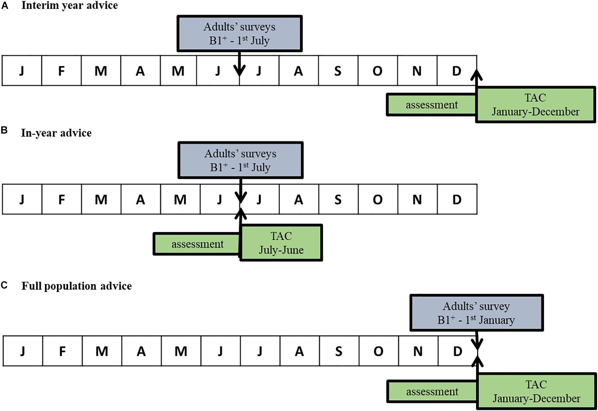
Figure 1. Graphical representation of the timings of abundance surveys, stock assessment and management period for each management calendar. From top to bottom, interim year advice, in-year advice and full population advice.
Following a similar approach to Sánchez et al. (2018), we evaluated two alternative management calendars than shortened the time lag between the biomass index and the management advice: in-year advice (iny) and full population advice (fpa). In the in-year advice, the management calendar was moved to July-June, and the TAC was set as soon as the biomass index on B1+ at the beginning of the second semester was available. So, the TAC from July (y) to June (y+1) was based on the index up to year y as follows:
This implies that the biomass index provided indications on the abundance of the age 1 group during the second semester in year y, but not during the first semester of year (y+1) (Figure 1B).
In the full population advice, the management calendar was the calendar year, but the biomass index was available up to year (y+1) and provided information on all the age classes that were going to be exploited (i.e., B1+ at the beginning of the first semester). The TAC from January to December (y+1) was:
This is the usual case when a recruitment index is available, and the TAC is set based on indications on all the age classes (Figure 1C). But it also applies to cases where a survey at the beginning of year y on B1+ will be used to set the TAC of the entire year y (even if the TAC is set once the management year has started).
Regarding the values of n and m, we tested the 2-over-3 rule that is the default ICES harvest control rule for category 3 stocks, and we compared it with respect to other rules that could potentially react faster to the high IAV of the short-lived fish stock dynamics, namely, 1-over-2, 1-over-3 and 1-over-5. In the first year of application of the rule, the rule depended on a reference TAC value, which was calculated as an average of the catch in the most recent m years, being m the number of preceding years in the denominator of the harvest control rule.
In the ICES framework for stocks in categories 3–6, to avoid large oscillations in the TAC advice from year to year, due to noise in the indices, the interannual changes in TAC advice are capped, so that only changes up to a maximum limit are allowed. The so-called Uncertainty Cap level (UC) has a default value of ±20%. This means that the TAC change from year to year cannot be larger than 20%, or if defined by the ratio of the consecutive TACs they must lie between 0.8 and 1.2. In general, if we denote UC(L,U) the uncertainty caps with L lower and U upper levels, the ratio of the consecutive TACs from year to year will be within the interval (1-L, 1+U). We considered the following alternative UCs: (i) no UCs denoted as UC(NA,NA); (ii) symmetric UCs at ± 20% UC(0.2,0.2), ± 50% UC(0.5,0.5) and ± 80% UC(0.8,0.8); and (iii) asymmetric UCs at 20% lower and 25% upper caps UC(0.2,0.25), 50% lower with 100% upper, UC(0.5,1.0), or with a 150% upper caps, UC(0.5,1.5), and 80% lower with 275% upper, UC(0.8,2.75), or with 400% upper UC(0.8,4) or with 525% upper caps, UC(0.8,5.25). In the case of the symmetric UCs, even when a decreasing change is followed by an increasing change of the same magnitude, the TAC does not achieve the same level, so that continuously applying the symmetric UCs up and down would lead to a continuous decrease in the TAC. The asymmetric UCs aimed at overcoming this by allowing larger upper than lower uncertainty caps to allow recovering to the same or larger TAC levels after a reduction. The UC values considered allow recoveries of the initial TAC levels up to: 75% for UC(0.5,0.5) and UC(0.8,2.75); 100% for UC(0.2,0.25), UC(0.5,1.0) and UC(0.8,4); and 125% for UC(0.5,1.5) and UC(0.8,5.25).
It is important to note that the n-over-m rules, without and with uncertainty caps, have intrinsic properties that determine the performance of the rule. As shown in Supplementary Annex II, for an abundance index in stationary conditions that fluctuated around its mean according to a log-normal error (σ2)distribution (accounting for both observation and process errors), any n-over-m ratio (rn,m) with n < m resulted in a median value <1 with the following expected value:
This means that these rules tended to reduce the fishing opportunities along time. In general, the larger the difference between n and m, the larger would be the reduction properties of the rule. In addition, the greater the interannual variability of the index, the greater the reduction properties of the n-over-m rule would be (up to an asymptotic value). The application of uncertainty caps generally modified the reduction properties of the rules. When symmetric uncertainty caps were incorporated (i.e., L = U), the reduction property was kept though its magnitude was modified and it could almost be vanished for small symmetric uncertainty caps (∼0.2). Alternatively, for asymmetric UCs, given a lower cap value (L), as the upper value (U) increased the change factor of the rule increased and large differences between the lower and upper value (U-L) turned over the rule properties from a reduction to an increase of the fishing opportunities. In fact, given the variability of the index and the parameters of the rule n, m and L, it would be possible to calculate what upper uncertainty cap level (U) is required to make the median change trend factor equal to either (i) the median change factor obtained without uncertainty caps, or (ii) to 1 (i.e., the inflexion point, where the factor turns from a reduction to an increasing factor).
For a subset of rules, we also evaluated the effect of including a biomass safeguard (Fischer et al., 2020). This consisted in a multiplicative factor that reduced the TAC advice when the observed index was below a threshold value (Itrigger):
where Il is the last available index and the biomass safeguard Itrigger can adopt three alternative values: Imin = min(Ihist); Iminpa = 1.64⋅min(Ihist) or Inorm = exp(mean(log(Ihist))−1.645⋅sd(log(Ihist))). The biomass safeguard was included in the 1-over-2 rule with (i) no UCs: UC(NA,NA); (ii) symmetric UCs at ± 20%: UC(0.2,0.2) and ± 80%: UC(0.8,0.8); and (iii) asymmetric UCs at 80% lower with 400% upper caps: UC(0.80, 4.00).
Implementation Model
No implementation error was simulated. All the TAC was taken as far as the population supported it. Catches were not allowed to be larger than 90% of the numbers at age in the population. The percentage of the TAC taken in each semester was set to 50%. When the semester quota was not taken, it was transferred to the next semester within the same management calendar.
Scenarios
For each combination of stock type and historical fishing pattern (2 stock types × 3 fishing patterns) we evaluated the performance of 120 variants of the advice rule (corresponding to 4 variants of the n-over-m advice rule, 10 sets of UCs and 3 management calendars). Simulated scenarios were the combination of the alternatives for the different components listed in Table 1.
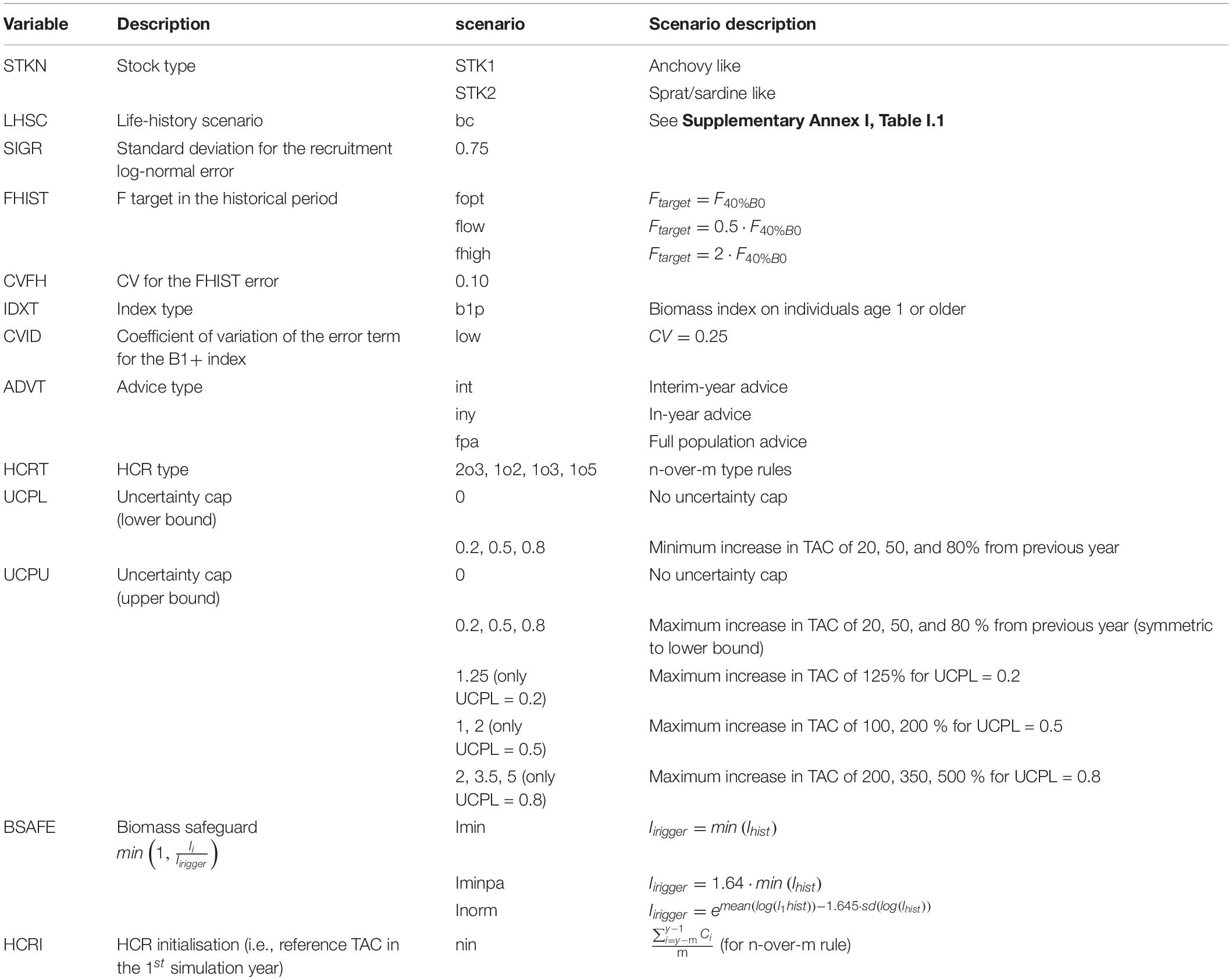
Table 1. List of alternative scenarios simulated for the different components.
Projections
Dynamics were simulated forward for 30 years and run for 1000 iterations for each scenario. Uncertainty in the projection period was introduced through: (i) recruitment process error from a Beverton and Holt stock-recruitment relationship; and (ii) the log-normal observation error on the B1+ index used to establish the TAC.
Performance Statistics
For each stock and starting depletion level, we calculated the interannual variation (IAV) of biomass as the average of the IAV of each iteration (IAViter):
where By, iter is the total abundance in mass at the beginning of year y and iteration iter and N is the number of years in the selected period. This statistic was calculated for the historical period (years 0–30), the short-term of the projection years (first five projection years; years 31–35) and the long-term of the projection years (last ten projection years; years 51–60).
For analysing the performance of the different rules under the alternative operating models, the biological risks (maximum probability of SSB being below the biomass limit Blim in the projection period) and the relative yields (ratio between catches and maximum sustainable yield MSY) were calculated in the short, medium and in the long-term. It must be noted that, according to the ICES precautionary criteria, biological risks are considered acceptable at or below 0.05.
Sensitivity Analysis
We tested the sensitivity of the rules’ performance to the coefficient of variation of the survey index (CVI). As an alternative to the assumed value of 0.25 that was considered a low CV, we considered a high CV equal to 0.5, a CV equal to the IAV in the historical period and a CV twice the IAV in the historical period. These last two cases aimed at exploring the signal-to-noise between the abundance index and the inherent variability of the population itself. The sensitivity analysis was carried out for the following subset of rules: (i) all the rules without any UC, to test the impact of the error in the index observation without any constraints in the TAC changes; and (ii) the 1-over-2 and the 2-over-3 rules with symmetric 80% UCs.
Robustness of the results with respect to the assumptions on the stock productivity and recruitment variability were also tested. Regarding the productivity, the steepness of the Beverton and Holt stock-recruitment model was changed to 0.5 (corresponding to low productivity) and to 1 (for high productivity). For the recruitment variability, values of the standard deviation of the recruitment model were set at 0.5 and 1. This sensitivity analysis was carried out for the following subset of rules: (i) the 1-over-2 rule without any UC; (ii) the 1-over-2 and the 2-over-3 rules with symmetric 80% UCs; and (iii) the 1-over-2 rule with 80% lower and 400% upper UCs.
Results
Life History Characteristics
The two types of stocks simulated had markedly different IAVs (Figure 2). Anchovy-like stocks (STK1) had significatively larger IAV than the sprat/sardine-like stocks (STK2). However, the IAV of a given stock was also a function of the initial depletion level (FHIST), the recruitment variability (SIGR) and to a lesser extent of the stock productivity. The IAV tended to increase as exploitation levels, recruitment variability or stock productivity increased.
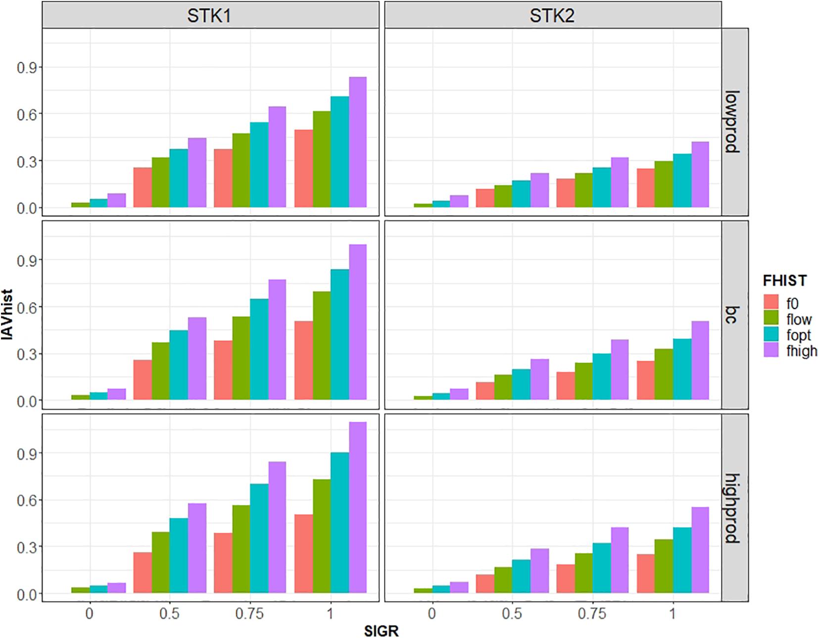
Figure 2. Interannual variation in the historic period (IAVhist) by standard deviation for the recruitment log-normal error (SIGR, x-axis) as a function of the stock type: anchovy-like (STK1) and sprat/sardine-like (STK2); stock productivity: low (lowprod), medium (bc) and high (highprod); and the exploitation level: zero catch (f0), under exploitation (flow), fully exploited (fopt) and overexploitation (fhigh). Interactive version of the figure is available online at https://aztigps.shinyapps.io/Sanchezetal2021_FMS/.
Given the alternative historical exploitation levels considered, the initial population status for the two stock-types was very different in terms of risks at the beginning of the projection period (Table 2). Initial risks were higher for the anchovy-like stocks. For the presumed optimum level of exploitation (Fproxy leading to 40%B0), the anchovy-like stock (STK1) had a high initial risk of falling below Blim (equal to 0.12), while for the sprat/sardine-like stock (STK2) this risk was 0.01. For the case of overexploitation initial risks increased to 0.4 and 0.3 respectively, while for the case of under exploitation initial risks were below 0.05 for both types of stocks. If the stocks were allowed to evolve without fishing during the projection period, short term risk for the anchovy was at or above 0.05 for the fully exploited and overexploitation trajectories, while for the sprat/sardine short term risk was above the threshold of 0.05 only for the historical overexploitation trajectory. These risks levels, in the absence of fishery, dropped to zero in the long-term for all the cases.
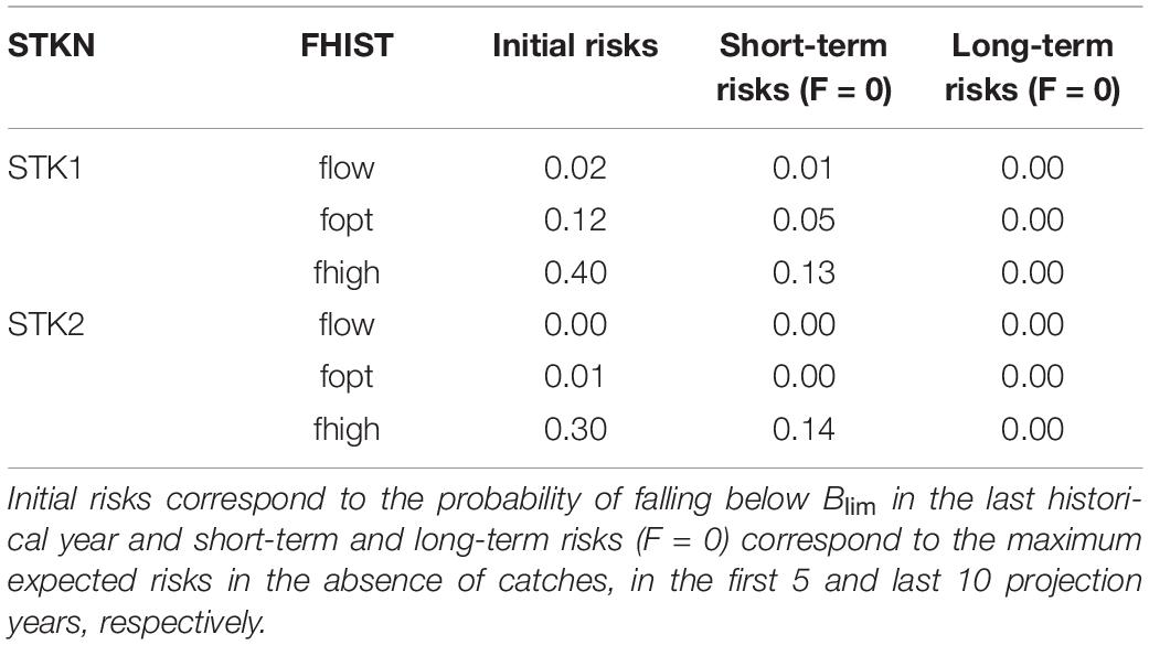
Table 2. Biological risks for the different OM conditionings (combination of stock -STKN- and initial depletion level -FHIST-) for base case productivity and recruitment standard deviation at 0.75.
Rules Comparison Under Base Case (Median Productivity and SIGR = 0.75)
For any given rule, the timing of the advice and management was a major factor in the performance of the rule, both in terms of yield and biological risks. The shorter the lag between observation and management (int > iny > fpa), the bigger were the expected relative yields and the smaller the risks (Figure 3). Generally, in-year advice (iny) outperformed the interim year advice (int) and full population advice (fpa) performed better than the other two, by resulting in smaller biological risks and larger relative yields. Although the differences between the iny and fpa advices were minor in comparison to their differences with the int. These effects were clearer in the long than in the short-term. Only in a few cases (mainly for anchovy-like stocks) the shortest time lag (fpa) did not improved the performance of the rules in comparison with the iny in the long-term. Most of these cases corresponded to the 1-over-m rules with lower 20% UC or the 2-over-3 rule without any UC, while for the few remaining cases differences were negligible. All the results from now on will be analysed for the in-year advice.
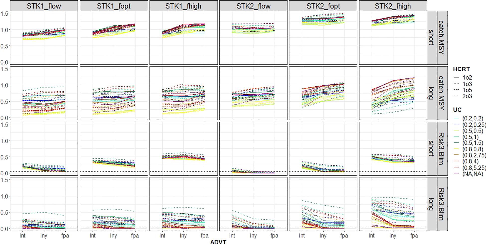
Figure 3. Relative yields (catch/MSY) and biological risks (Risk3.Blim: maximum probability of falling below Blim) by calendar type (ADVT, x-axis) and alternative operating models (in columns). The harvest control rules (HCRT) are represented by line types and uncertainty caps limits (UC) by line colours. See Table 1 for definitions of abbreviations. The horizontal black dashed line represents the 0.05 biological risk. Interactive version of the figure is available online at https://aztigps.shinyapps.io/Sanchezetal2021_FMS/.
Figure 4 shows the median trajectories for the two simulated stocks for the standard advice rule for ICES category 3 stocks, namely the 2-over3 rule with a 20% uncertainty cap. During the projection period, median SSB increased, except for historically overexploited (fhigh) sprat/sardine-like stock for which the stock showed a high and increasing probability of collapse during the projection period (Figure 4). However, in all the cases, the variability of the SSB trajectories was very high, leading to large biological risks in the short-term (between 0.16 and 0.46 for anchovy-like stocks and between 0.01 and 0.44 for sprat/sardine-like stocks, depending on the initial exploitation status) which were reduced in the long-term for the anchovy-like stocks (to values between 0.09 and 0.27), but were increased for the sprat/sardine-like stocks (to values between 0.02 and 0.52). In all the cases, catch decreased through the time series with the median always remaining below MSY during the projection period (Figure 4).
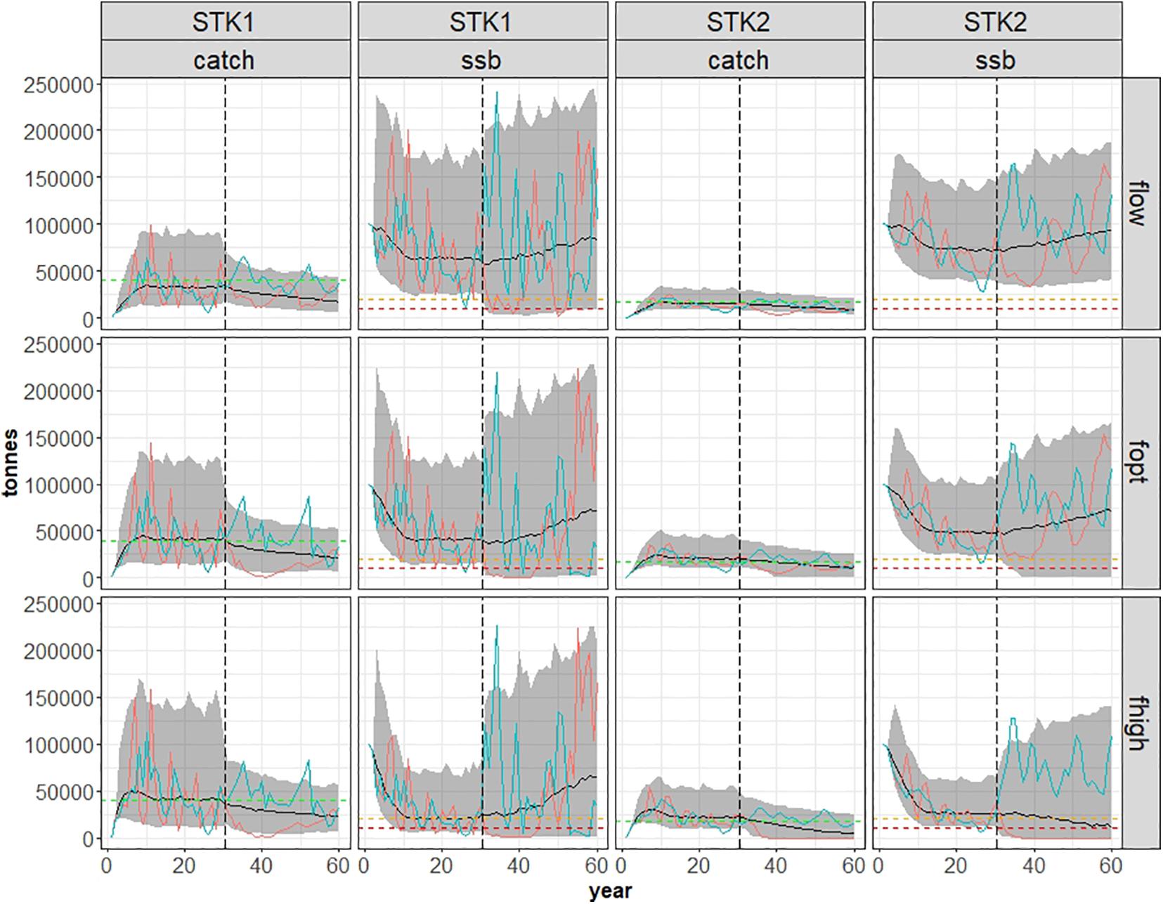
Figure 4. Trajectories of catch and SSB in tonnes along years (x-axis) for the 2-over-3 rule with a 20% uncertainty cap and under an in-year advice for different life histories: stock-types in columns and historical exploitation levels in rows. The solid line represents the median and the shaded area the 90% confidence intervals computed from the 5th and 95th percentiles and coloured lines represent specific iterations. The dashed vertical line is located before year 31, which is the first year of the projection. The dashed horizontal lines represent the different reference points: the green line in catch plots correspond to MSY and orange and red lines in SSB plots to Blim (20% B0) and Bcollapse (10% B0), respectively. Interactive version of the figure is available online at https://aztigps.shinyapps.io/Sanchezetal2021_FMS/.
In comparison to the other rules, for the same UC levels, advice rule 2-over-3 resulted in higher risks in the long term (Figure 5), and generally above 0.05 (with the only exception for both stocks of using UC(0.8,0.8)). Moreover, the 20% symmetric uncertainty cap, used as a standard in ICES, resulted in risks above 0.05 at historical exploitation levels at or above FMSY for both stock-types and for any trend rule.
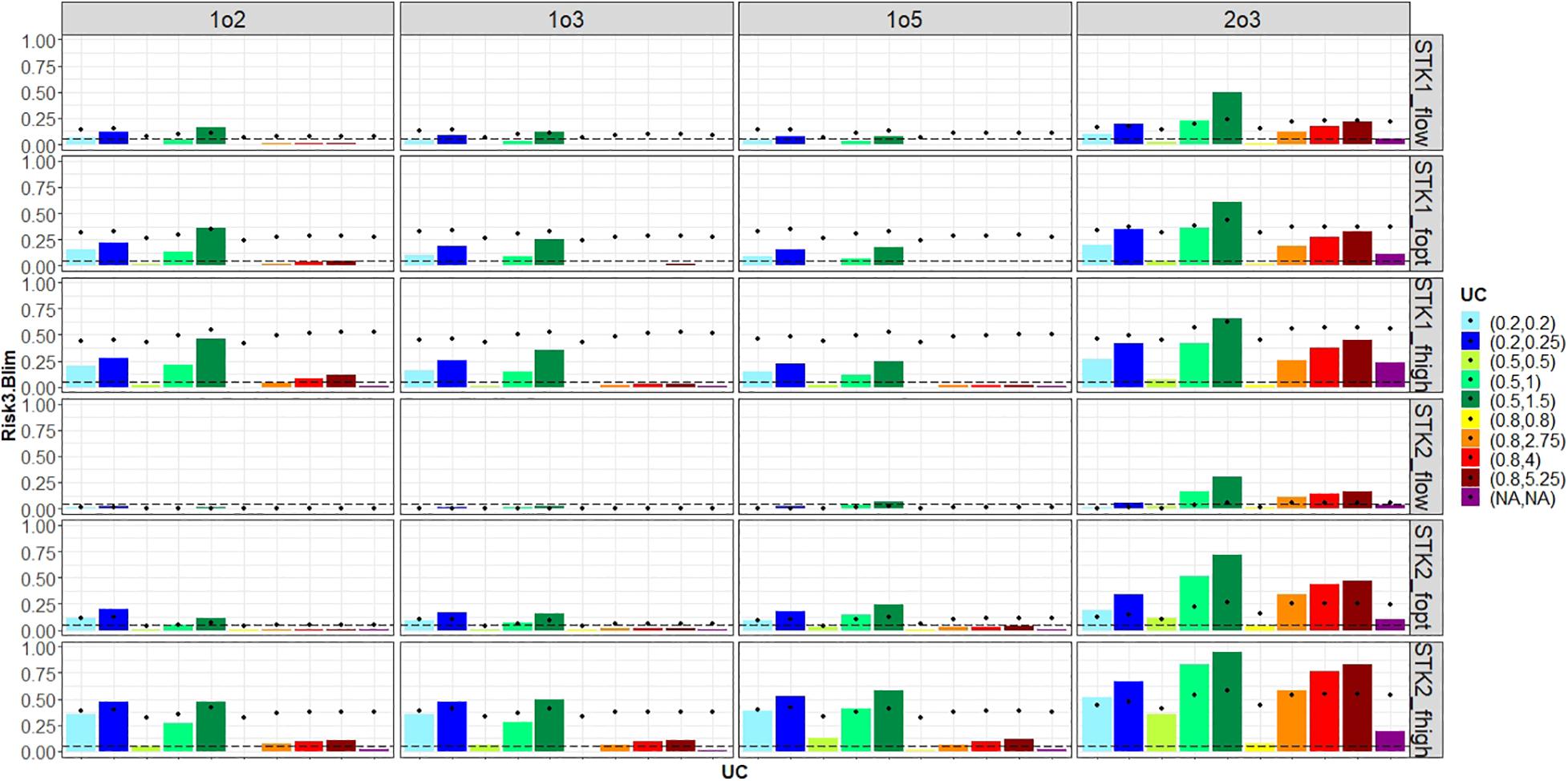
Figure 5. Biological risks (Risk3.Blim: maximum probability of falling below Blim) for the different configurations of the rule in an in-year advice. The rows correspond to the operating models (combination of stock type and the historical exploitation level) and the columns to the harvest control rule type. The uncertainty cap lower and upper limits combinations are represented on the x-axis for alternative timeframes: the black dots represent the risks in the short-term (first 5 projection years) and the colour bars represent the risk in the long-term (last 10 projection years). The horizontal dashed line corresponds to the 0.05 risk. See Table 1 for definitions of abbreviations. Interactive version of the figure is available online at https://aztigps.shinyapps.io/Sanchezetal2021_FMS/.
In the short-term, differences in the rules’ performance were small both in terms of in terms of risks (Figures 5, 6) and yield (Figure 7). For all the rules tested, initial depletion levels were the major drivers of risks in the short-term. As historical fishing mortality increased, risks increased. For the historical exploitation levels above FMSY all the rules resulted in short-term risks well above the 0.05 precautionary level. This was also seen for the anchovy-like stock (STK1) exploited at an optimum exploitation level, where short-term risks were also above 0.05. In the long term, for every UC level and historical exploitation, rule 2-over-3 had equal or larger relative yield than the 1-over-m respective rules but always with higher risks. Differences among the other rules (1-over-m rules) were smaller in terms of catches and risks at equal UC and historical exploitation level, though in general for the 1-over-m rules, there was a small reduction of catches and risks for the anchovy-like stocks as m increased and just the contrary (increased with m) for the sprat/sardine-like stocks. In most cases, the 1-over-m rules reduced the risks along time (Figure 6), except when applied to fully or overexploited sprat/sardine-like stocks coupled with the UC(0.2,0.25) or UC(0.5,1.5). Alternatively, the 2-over-3 rule did not reduce risks as much as the 1-over-2 rule, and could even result in increased risks particularly for the sprat/sardine-like stocks (except for UC(0.8,0.8) or UC(NA,NA)).
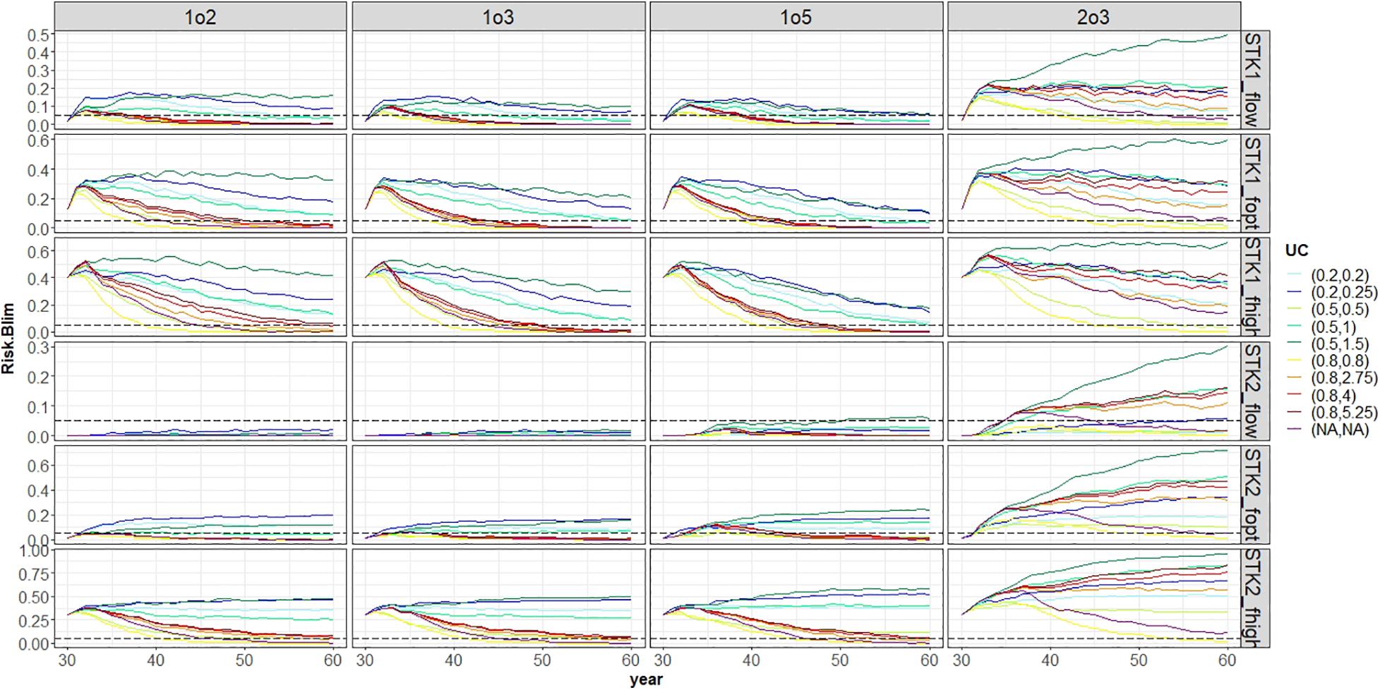
Figure 6. Trajectories of biological risks (Risk3.Blim: maximum probability of falling below Blim) along years (x-axis) under an in-year advice. The rows correspond to the operating models (combination of stock type and the historical exploitation level) and the columns to the harvest control rule type. The uncertainty cap lower and upper limits combinations are represented by different coloured lines. The horizontal dashed line corresponds to the 0.05 risk. See Table 1 for definitions of abbreviations. Interactive version of the figure is available online at https://aztigps.shinyapps.io/Sanchezetal2021_FMS/.
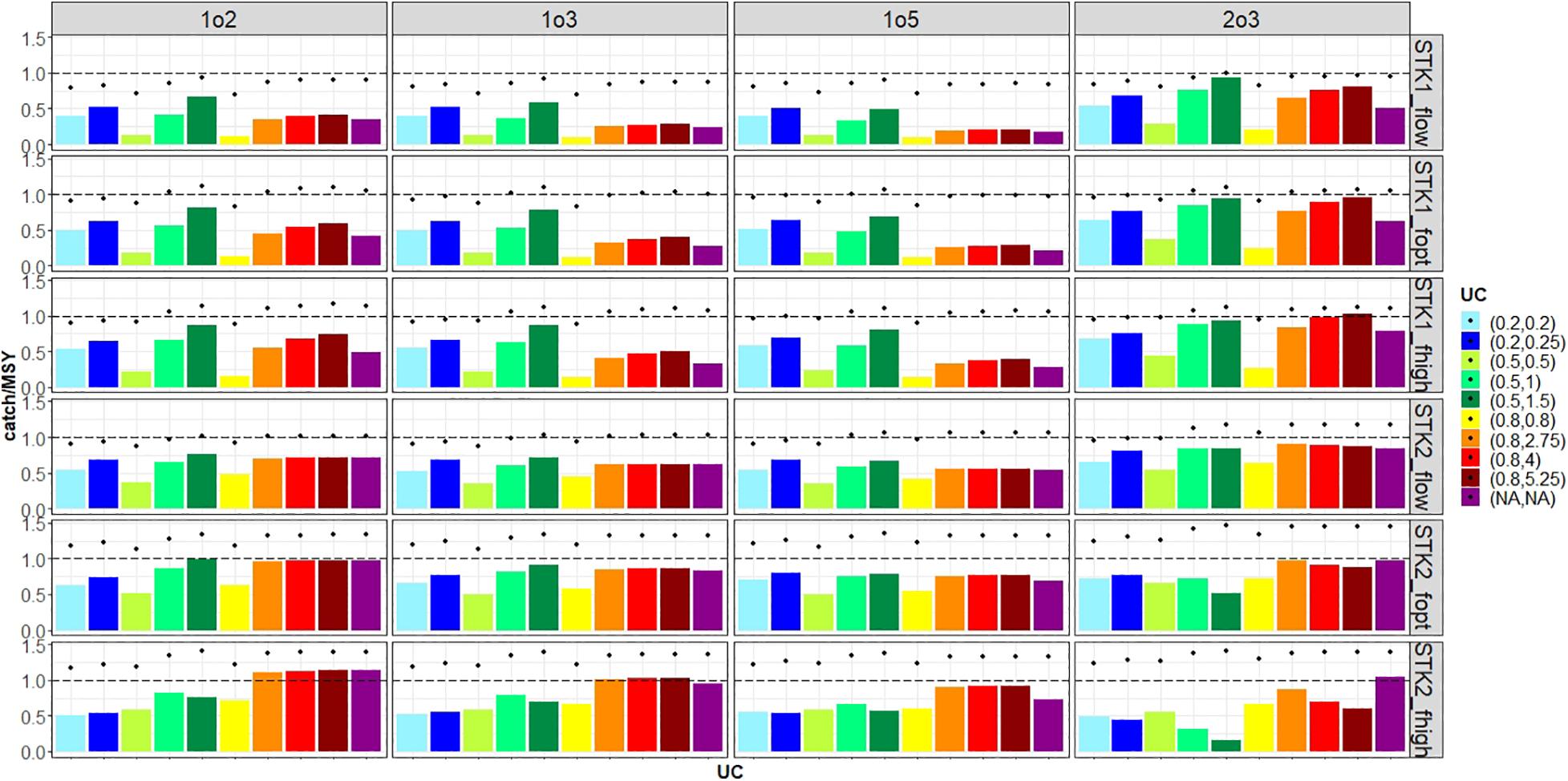
Figure 7. Relative yields (catches/MSY) for the different configurations of the rule in an in-year advice. The rows correspond to the operating models (combination of stock type and the historical exploitation level) and the columns to the harvest control rule type. The uncertainty cap lower and upper limits combinations are represented on the x-axis for alternative timeframes: black dots represent the relative yields in the short-term (first 5 projection years) and the colour bars represent the relative yields in the long-term (last 10 projection years). The horizontal dashed line corresponds to catches at MSY. See Table 1 for definitions of abbreviations. Interactive version of the figure is available online at https://aztigps.shinyapps.io/Sanchezetal2021_FMS/.
Regarding the effect of the different UCs, for every rule asymmetric UCs had higher relative yields and risks in the short term compared to those with symmetric UC. For the same lower uncertainty cap, the larger the upper uncertainty cap (i.e., the larger the asymmetry), the larger the risks for similar or larger catches. However, differences were small in terms of relative yields for the lower UC (UCL) at 80% (Figure 7). Largest risks were usually seen for the UC(0.5,1.5) as it tended to result in the largest allowed catches (Figure 5). These effects were amplified in the long term: for all scenarios defined by stock type, historical exploitation level and trend rule, the asymmetric UCs had higher risks than those with symmetric UC and were not always accompanied with higher relative yields. Among the symmetric UCs, UC(0.2,0.2) is the one resulting in highest risks (not always with highest relative yields). UC(0.2,0.2) was non-precautionary regardless the type of HCR (Figure 5) for all the OMs, except for the sprat/sardine-like stocks with low historical exploitation levels. For the symmetrical UCs, long-term results showed that in general the larger the interannual percentage of change allowed, the smaller were the risks and, to a lesser extent, the catches, up to the 80% UC. If unconstrained (no UCs), risks showed a sharp decrease along with a relatively minor decrease in catches. The differences in terms of risks between the performance of the rules 1-over-m with 80% symmetric UC and without any UC was minor compared to the increase of catches of the latter case (no UCs). If focusing only on the symmetric UCs, the only rule that was precautionary in the long-term for all simulated OMs was the 1-over-2 rule without any UC or with a symmetric 80% UC. However, the 1-over-2 rule without UC (unconstrained changes) resulted in similar risks for substantially higher catches.
When comparing across all rules in terms of the trade-off between yields and risks, the best rule was the 1-over-2 without any uncertainty cap, as for all OMs it resulted in the highest levels of catches for sustainable risk levels in the long term (Figure 8). Subtle differences between stocks might be seen, as for the anchovy-like stocks (STK1) the 1-over-2 rule with UC(0.8,2.75) resulted in slightly higher catches for precautionary level of risks, while for the sprat/sardine-like stocks (STK2) the 1-over-2 rule without any uncertainty cap was the rule producing highest yields for slightly smaller risks. The figure also shows that if in the long-term risks below 0.1 would be acceptable, then 1-over-2 rule with UC(0.8, 4) would result in the largest catches for all OMs keeping risks below 0.1. Overall, this means that for these short-lived fish stocks with base case population dynamics 1-over-2 rule was preferred and should be applied with a large uncertainty cap (as large as UC(0.8,2.75) or UC(0.8,4)) or without setting it, UC(NA,NA), to achieve the best compromises between risks and catches in the long term.
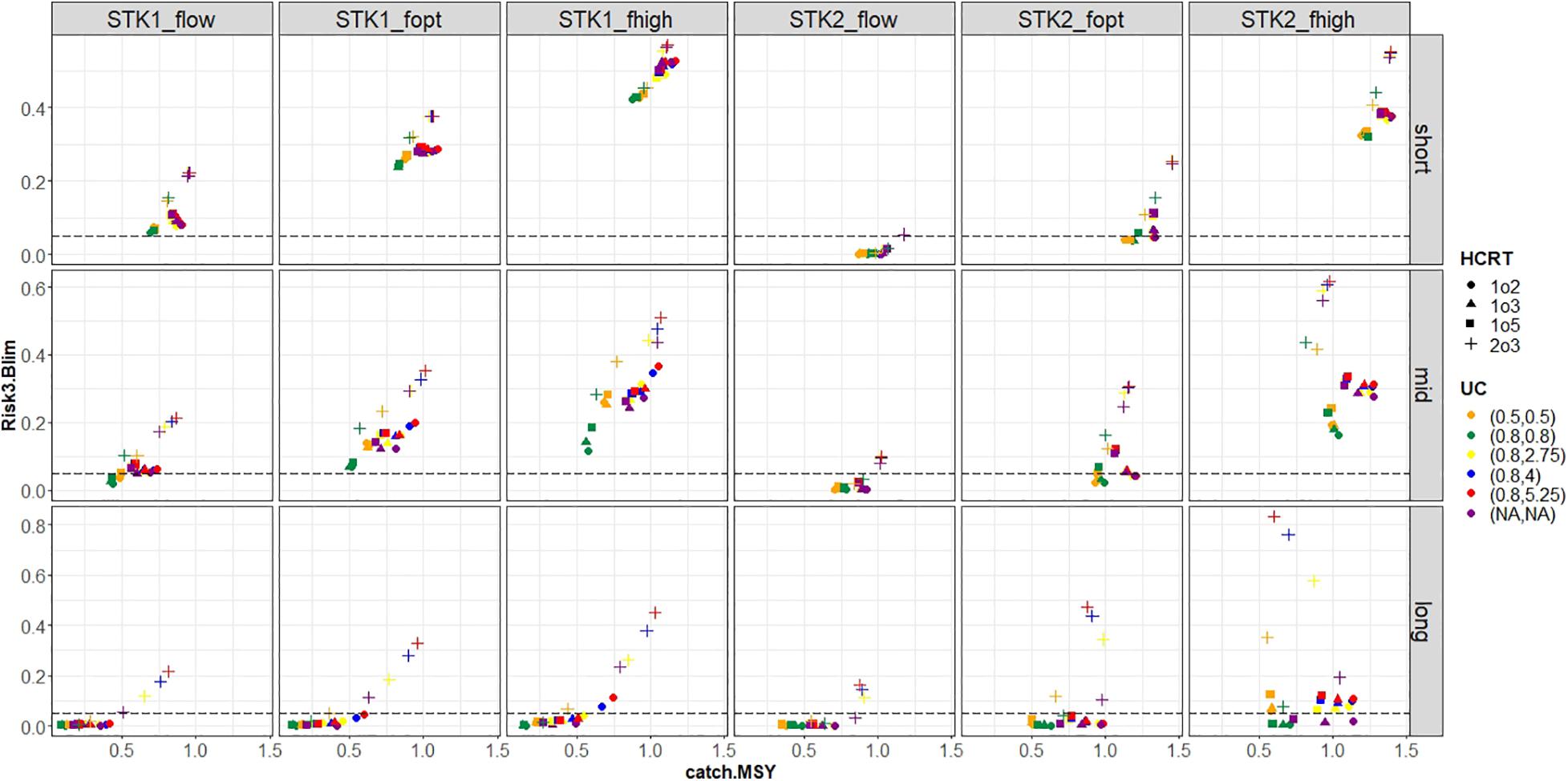
Figure 8. Biological risks (Risk3.Blim: maximum probability of falling below Blim) versus the relative yields (catches/MSY) (x-axis) by rule type (symbols) and uncertainty cap lower and upper limits (colours). The columns correspond to the different OMs (as combination of the stock-type and historical exploitation) and the rows to the temporal scales: the short-term (first 5 projection years), medium-term (next 5 projection years) and the long-term (last 10 projection years). Dashed line corresponds to the 0.05 risk. See Table 1 for definitions of abbreviations. Interactive version of the figure is available online at https://aztigps.shinyapps.io/Sanchezetal2021_FMS/.
The inclusion of a biomass safeguard in the rules remarkably reduced the risks in the medium and long terms by slightly reducing the relative yields for the fully or overexploited stocks (Figure 9). However, the 1-over-2 rule without UC and without biomass safeguard was still among the rules showing the best compromise in catches over risks in the long term for all OMs, complying always with the ICES precautionary criteria. The Inorm biomass safeguard lead to the smallest reduction in relative yields with similar benefits in the reduction of risks as Imin, whilst Iminpa implied bigger loses in yield for very similar risks. In the long term, the asymmetric UC(0.8,4) turned to be precautionary regardless the initial exploitation level when combined with a biomass safeguard. Additionally, the biomass safeguard made the UC(0.2,0.2) precautionary in the long-term. Notably the major differences were driven by the uncertainty cap limits, whereby the symmetric UC(0.8,0.8) implied greater reduction of risks than the others (particularly clear in the medium term). Focussing on the medium term the faster reduction of risks was achieved by rule 1-over-2 with UC(0.8,0.8) and a biomass safeguard of Iminpa.
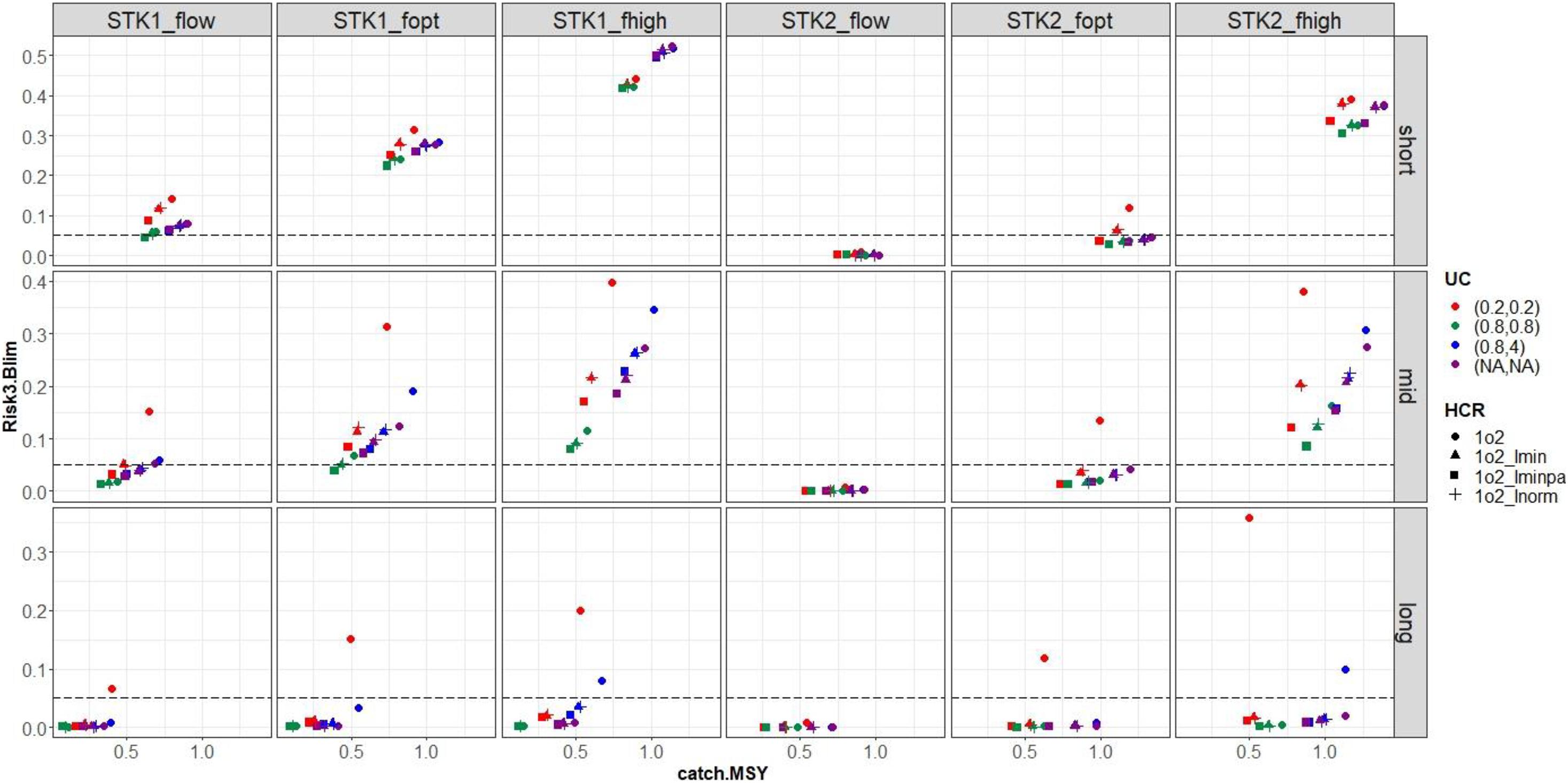
Figure 9. Biological risks (Risk3.Blim: maximum probability of falling below Blim) versus the relative yields (catches/MSY) (x-axis) for the 1-over-2 rule by uncertainty cap lower and upper limits (colours) and biomass safeguards (colours). The columns correspond to the different OMs (as combination of the stock-type and historical exploitation) and the rows to the temporal scales: the short-term (first 5 projection years), medium-term (next 5 projection years) and the long-term (last 10 projection years). Dashed line corresponds to the 0.05 risk. See Table 1 for definitions of abbreviations. Interactive version of the figure is available online at https://aztigps.shinyapps.io/Sanchezetal2021_FMS/.
Sensitivity to Coefficient of Variation of the Survey Index
For all the n-over-m rules without any UC and the 1-over-2 and 2-over-3 rules with symmetric 80% UCs, when the CV of the index increased, the relative yield decreased (Figure 10). While, in the case of risks, different patterns were observed depending on stock type and rules. For underexploited anchovy-like stocks and under- or fully exploited sprat/sardine-like stocks, risk increased as CV increased, whereas for the rest of operating models risks decreased or stayed almost unchanged as CV increased. This pattern was more marked for the 2-over-3 rule without UC. However, observed small reduction in risks in the long-term occurred at the expense of a significant reduction in catches. All these effects must be related to the fact that observation errors in surveys implied increased perceived variability of the population (actually , where IAVobs is the observed IAV, IAVOM is the IAV in the population and CVID is the index CV) and this perceived IAV increase induced more pronounced reduction properties of the rules (Supplementary Annex I). If the reductions in risks were less relevant than reduction in catches, it was probably related to a poorer signal to noise ratio in the observations of the population when CV of the survey (CVID) increased. In summary, the increase in CVs tended to decrease expected catches because they amplified the reduction properties of the rules through increased perceived IAV, but did not necessarily reduce risks because of the poorer signal to noise information (particularly evident in the sprat/sardine like stock).
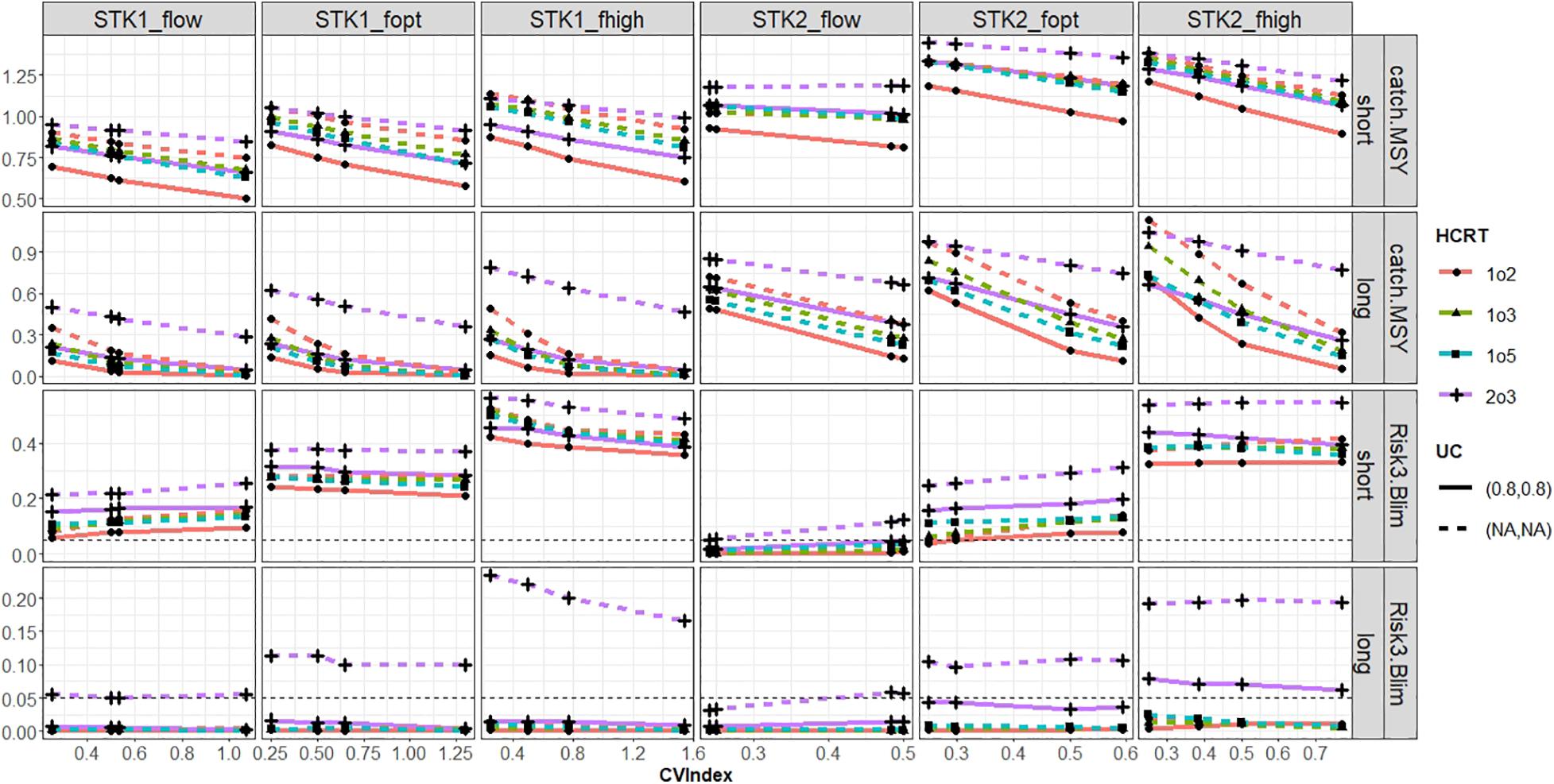
Figure 10. Relative yields (catch/MSY) and biological risks (Risk3.Blim: maximum probability of falling below Blim) in the short- and long-terms (in rows) under an in-year advice for the different CV values of the index (x-axis). The columns correspond to the operating models (combination of stock type and the historical exploitation level). The harvest control rule types are represented by the coloured lines and the uncertainty cap lower and upper limits combinations are represented by the line types (solid line: 80% symmetric uncertainty cap; and dashed line: 20% symmetric uncertainty cap). The horizontal dashed line corresponds to the 0.05 risk. See Table 1 for definitions of abbreviations. Interactive version of the figure is available online at https://aztigps.shinyapps.io/Sanchezetal2021_FMS/.
Risks increased almost linearly with the IAV (Figure 11). In general, the sprat/sardine-like stocks had smaller IAVs than anchovy-like stocks, but at similar IAVs anchovy-like stocks had smaller risks than sprat/sardine-like stocks (Figure 11). This was due to the fact that sprat/sardine-like stocks had similar IAVs as anchovy-like stocks only after being historically overexploited (i.e., when the stock was at rather low levels and risks were high), whereas anchovy-like stocks were underexploited (at flow, high biomass levels and low risks). The close relationship between risk and IAV by stocks was very clear in the short term, but in the long term and as a result of a large reduction in the catches, fishing mortality and IAV were greatly reduced.
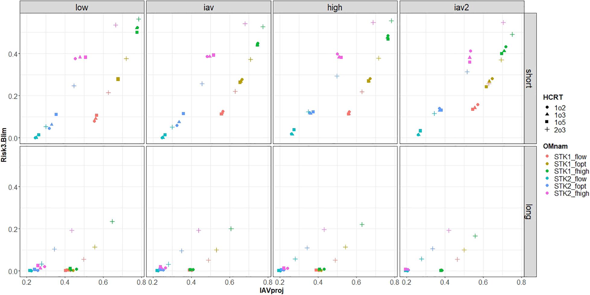
Figure 11. Biological risks (Risk3.Blim: maximum probability of falling below Blim) versus the interannual variability (x-axis) under an in-year advice. The columns correspond to the CVs of the index and the rows to the timeframes: the short-term (first 5 projection years) and the long-term (last 10 projection years). The harvest control rule types without any uncertainty cap are represented by the dot types and the operating models (combination of stock-type and historical exploitation level) are represented by the dot colours. See Table 1 for definitions of abbreviations. Interactive version of the figure is available online at https://aztigps.shinyapps.io/Sanchezetal2021_FMS/.
Sensitivity to the OM Assumptions
For the selected harvest control rules (2-over-3 UC(0.8,0.8) and 1-over-2 rule UC(0.8,0.8), UC(0.8,4.0) and UC(NA,NA)), when the standard deviation of the recruitment increased, risks in the long-term increased for under- or fully exploited stocks; whilst, for overexploited stocks, risks decreased as the standard deviation increased (Figure 12). Regarding catches, relative yields tended to decrease, at any historical exploitation level, as the standard deviation of the recruitment increased, except for the case of sprat/sardine-like stocks under the 1-over-2 rule with either UC(0.8,4) or UC(NA,NA), where the relative yields increased (Figure 13).
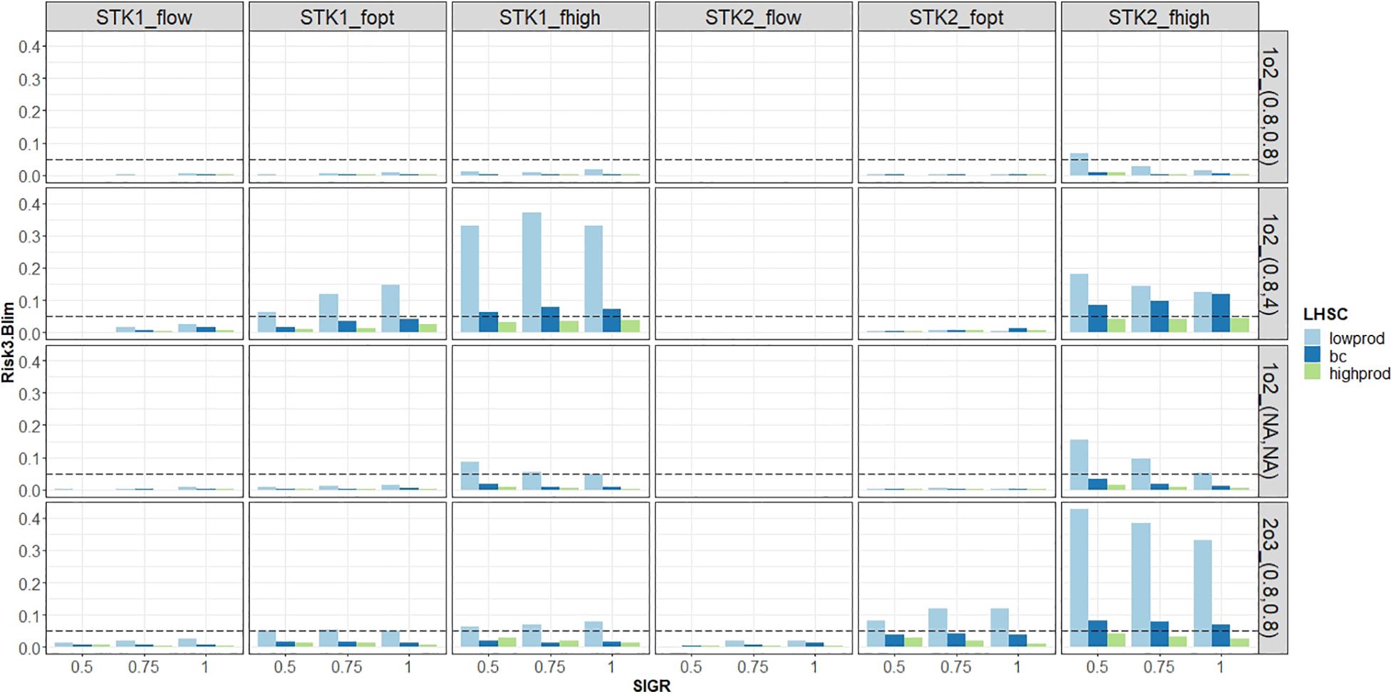
Figure 12. Biological risks (Risk3.Blim: maximum probability of falling below Blim) in the long-term (last 10 projection years) versus the standard deviation of recruitment (x-axis) and stock productivity (colours) under an in-year advice. The columns correspond to the alternative OMs (as combination of the stock-type and historical exploitation) and the rows to the configurations of the rule (harvest control rule type and uncertainty cap lower and upper limits). Dashed line corresponds to the 0.05 risk. See Table 1 for definitions of abbreviations. Interactive version of the figure is available online at https://aztigps.shinyapps.io/Sanchezetal2021_FMS/.
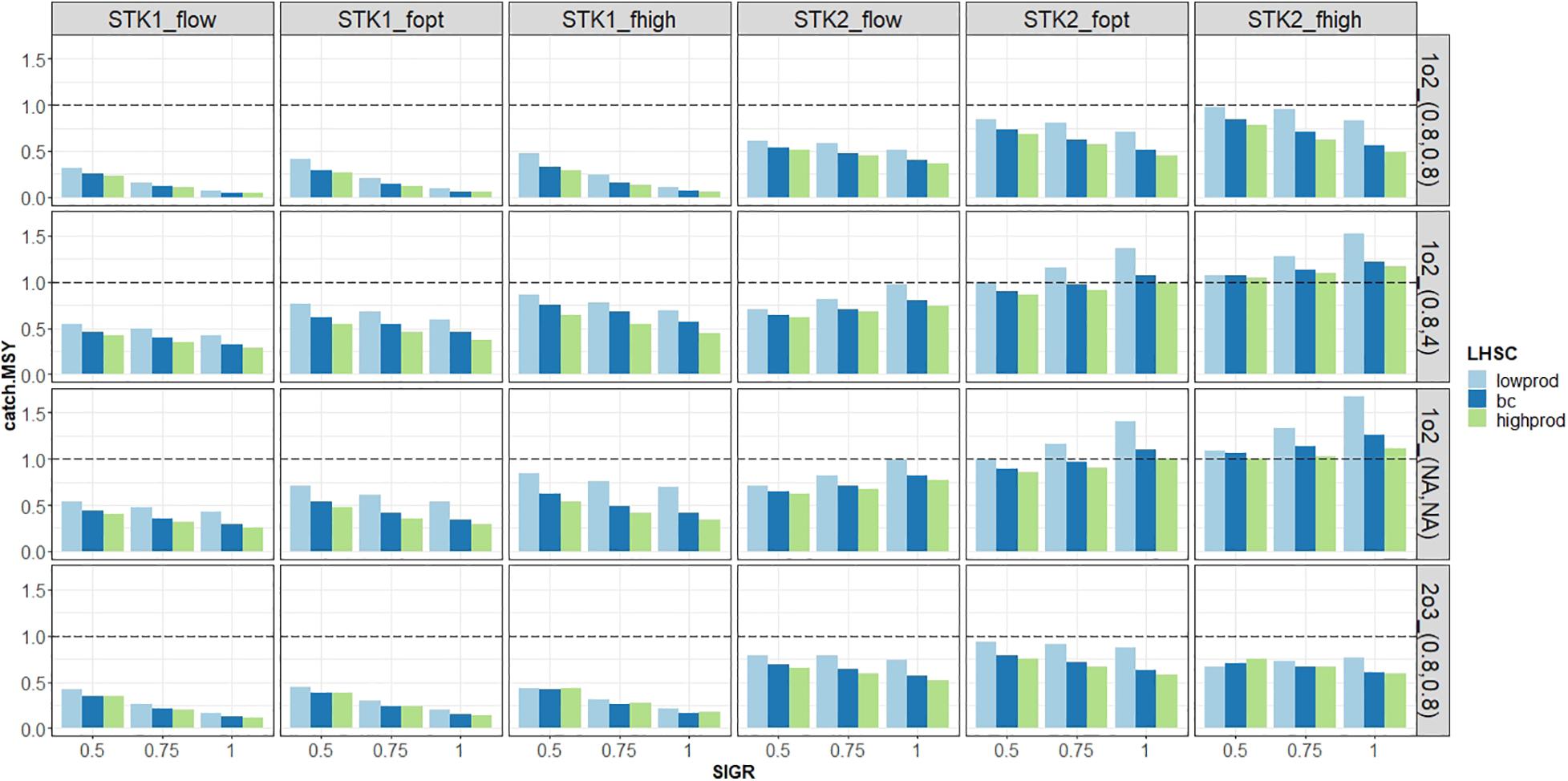
Figure 13. Relative yields (catches/MSY) in the long-term (last 10 projection years) versus the standard deviation of recruitment (x-axis) and stock productivity (colours) under an in-year advice. The columns correspond to the different OMs (as combination of the stock-type and historical exploitation) and the rows to the configurations of the rule (harvest control rule type and uncertainty cap lower and upper limits). Dashed line corresponds to catches equal to MSY. See Table 1 for definitions of abbreviations. Interactive version of the figure is available online at https://aztigps.shinyapps.io/Sanchezetal2021_FMS/.
Regarding the sensitivity to the productivity level, in the long-term, relative yields and risks decreased as productivity levels increased. The reduction in risks was greater than those observed in catches (Figures 12, 13).
Discussion
In this work we have tested by simulation the performance of the ICES advice rules for category 3 stocks for the case of short-lived fish. The default 2-over-3 rule with 20% UC (ICES, 2012a) resulted to be not precautionary as it implied long term biological risks above 5%. As an alternative, 1-over-2 rule unconstrained by any uncertainty cap or the 1-over-2 rule including a biomass safeguard with 80% lower and 400% upper uncertainty caps accommodated better to the highly fluctuating nature of the short-lived stocks, resulting in precautionary risk levels in the long term.
In the last years, empirical harvest control rules that set the management actions based on directly observable indicators rather than from stock assessment models are increasingly being proposed for data-limited stocks (Bentley and Stokes, 2009a; Dowling et al., 2015). In particular, empirical rules that included an abundance index providing a precise estimate on stock status have been shown to perform better than those that lack such an index (Carruthers et al., 2014; Geromont and Butterworth, 2014). The catch trend rules considered in this work, including the ICES advice rule for category 3 stocks, are within this type of empirical harvest control rules and they aim at managing the stocks by modifying the advice according to changes in stock status obtained from an abundance index. However, for a short-lived fish the value of any index would be limited in time as the populations are largely renewed year after year according to the strength of recruitment. For this reason, the guidance provided by any index on the target managed population degrades with time and can become misleading if the fraction of the managed population informed by the index is not sufficiently representative. This explains why a key factor determining the performance of the rules for short-lived fish was the time lag between the abundance index and the management calendar. From the three management calendars evaluated, the shorter the time lag between the observed index and the application of the management advice, the bigger were the catches and the smaller were the biological risks. In the interim year advice, there was a time lag of about a year between the index and the management calendar, so that the TAC was set without any indication of the age 1 class which would form the bulk of the population. Moving the management calendar to July-June, as soon as the abundance indices were available, allowed for the in-year management to reduce this time lag to just half a year and allowed gaining information on all age classes sustaining the second half of the year catches and all except age 1 of the next (first) half of the following year catches. This in-year management procedure has been applied successfully in the case of the Bay of Biscay anchovy where, after the stock collapse in 2005, such a change in the management calendar allowed to reopen the fishery with a management plan based on the most recent biomass estimates from the spring fishery independent surveys (Sánchez et al., 2018). Other successful applications are the joint management procedure for the multispecies South African pelagic fishery where a within-season revision of the anchovy TAC based on the most recent surveys allowed a better utilisation of the anchovy resource (De Oliveira and Butterworth, 2004) or the Australia’s Prawn Fisheries where the timing of the fishing season was adjusted during the year based on the assessed status of one of the tiger prawn species (Dichmont et al., 2006b; Anon, 2014, 2018). Interim and in-year advices have been also compared by Fischer et al. (2020), who found that including more recent data and setting the TAC yearly improved the performance of the empirical catch rule. The full-population advice calendar, in which the abundance index provides information on all exploited age classes over the entire management year, as for instance when a pre-recruit survey index is available, entailed further improvements with respect to the other management calendars. Early indication of recruitment strength have already been demonstrated to be beneficial in other works (Dichmont et al., 2006a; Le Pape et al., 2020). However, the improvement over the in-year procedure was smaller than that between the interim and the in-year advice procedures. For the Bay of Biscay anchovy, Sánchez et al. (2018) showed that the benefit of the full population advice procedure over the in-year advice was also moderate, as catches increased by 15% for the same level of allowable risks.
In relation with the former considerations, we expected that the 1-over-m rules would have a better performance (compromise between risks and relative yields) in managing these short-lived fish than the 2-over-m rules, as the later would incorporate in the numerator the obsolete index of year (y-1), hence not improving the information on the managed population. Furthermore, the 2-over-3 rules had lesser reduction properties of fishing opportunities in time than the 1-over-m rules. This was confirmed when comparing the rule 2-over-3 by UCs with any of the 1-over-m rule for the same stock and historical exploitation, as the latter achieved a substantial reduction of risks for lesser reductions of catches in all cases. The poor performance of this rule for the simulated stocks was in agreement with (Fischer et al., 2020) who demonstrated that the 2-over-3 rule performed very poorly for more productive stocks (i.e., with k > 0.32 year−1), which was the case of our simulated short-lived fish stocks (with k = 0.89 and k = 0.56 for anchovy-like and sprat/sardine-like stocks, respectively). By definition, the 2-over-3 rule smooths interannual changes in the stock indicator to obtain stock trends over the last five years, but for short lived species interannual changes are usually far larger than the medium-term trends in the stock and therefore 1-over-m rules have the power of better updating to the interannual changes conditioned to in-year advice management procedure. Rule 2-over-3 with UC(0.2,0.2) was devised at preventing the advice to push the exploitation to unlikely high or low levels because of abnormally high noisy observations. However, it was developed for stocks with lower interannual variability (stocks with longer lifespans which have substantial inertia over time) and therefore was not able to accommodate the high natural interannual fluctuations characteristic of the short-lived fish stocks (Barange et al., 2009; Checkley et al., 2017). As an alternative, the 1-over-m rules (those which select only the latest survey index in the numerator) were more reactive to the biomass fluctuations.
In general, the performance of the three 1-over-m rules tested were very similar within stocks, with some tendency of faster reduction of catches as m increased leading in the long term to smaller catches for both stocks for the larger m rules for all UCs (less intense in the sprat/sardine-like stocks) and to decreased risks but only for the anchovy-like stocks. The reasons for the different behaviour of the rules was partly related to the reduction properties of the rules (Supplementary Annex II). For instance, the tendency among the 1-over-m rules to produce smaller catches as m increased for slightly smaller levels of risks was a direct result of such mechanistic reduction properties, because the reduction effects for a fixed n became more pronounced as m increased. In addition, the stronger reduction of relative catches and risks for anchovy than for sardine/sprat like stocks for the same harvest control rules was a direct effect of the larger IAV of the anchovy-like stocks, because the larger the IAV the larger the reduction of the fishing opportunities in time produced by the rules.
Among these rules, we have seen that those with more restrictive UC (i.e., UC(0.2, 0.2) or UC(0.2, 0.25)) or with asymmetrical lower 50% UC (that is UC(0.5,1) or UC(0.5,1.5)) resulted in the poorest performance in terms of risks. The asymmetric rules with UCL of 50% (with UCU > UCL as tested here) were much more restrictive in reducing the catch options (as a maximum reduction of 50% was allowed) compared to facilities to increasing catches (with allowed increase up to 100% or 150%), diminishing the decreasing properties of the 1-over-m rules in comparison with the unconstrained application of the rules (i.e., UC(NA,NA)) or with the rest of the rules. The UC(0.5,0.5) resulted in lower catches and risks since such UC range increased the reduction properties of the rule compared to the unconstrained application (see further evidence in Supplementary Annex II). In general, larger UCs were expected to have an increased capability to accommodate the advice to rapid stock fluctuations. Our results supported this conclusion as for all rules of the type 1-over-m, the widest UC ranges (UC(0.8,∗)) resulted in smallest risks in the long term (always below 0.11) with the highest relative yields (i.e., catches/MSY). It is remarkable that no application of any uncertainty cap, UC(NA,NA), resulted in a robust rule which was sustainable in the long term for the two stocks or for any past historical exploitation of the stock, with allowable catches in the long-term as high as those allowed by UC(0.8,2.75). This result questions the need of any UC for short-lived fish species.
The addition of a biomass safeguard to the rules increased the reduction properties of the rules: faster with the Iminpa in the medium term, but with better balance between catch options for precautionary risk levels with the Inorm in the long term. The inclusion of the Inorm biomass safeguard allowed increasing the upper UC limit up to 400% (1-over-2 with UC(0.8,4) and Inorm), still precautionary for all the stocks independently of their starting depletion level, but not overcoming the balance showed in the long term by the unconstrained 1-over-2 (UC(NA,NA)).
Consequently, the balance between catches and risks (or risk per ton caught) favoured the adoption of the rule 1-over-2 rule, versus the 1-over-3 and 1-over-5 rules. Furthermore, in the medium term the best uncertainty caps associated to that rule were those with UC(0.8,0.8), while in the long term performed best with no UC (unconstrained, UC(NA,NA)) or with UC(0.8,4) when coupled with the Inorm biomass safeguard. The former indications are applicable to any short-lived fish as we have shown them to be robust to the different stock types and historical exploitation levels of the stock before management. However, we have seen that the optimum combination of rule type and UCs depended partly on the stock life-history characteristics. This means that, when possible, it would be desirable to identify which is the best harvest control rule for each case study by simulation testing (as defined by the combination of the trend rule, the UC and the biomass safeguard). Therefore, our current work serves for providing general guidelines, but it is still recommended, when available knowledge on the stocks allows it, to fine-tune the rules, as suggested by several authors (Walsh et al., 2018; Fischer et al., 2020). Carruthers et al. (2016) suggested that often tuning MPs for specific stocks is important, though this may not be viable in data-poor assessment scenarios because of insufficient data and analysis resources, as for instance in Sagarese et al. (2019).
None of the trend rules we have tested can assure in the short and medium terms that biological risks will be lower than 5%, as this would basically depend upon the initial depletion levels, though in the long term many of these rules became precautionary. Therefore, the selection of any rule should be based more on the relative performance of these rules in time (i.e., on the speed of reducing risks to precautionary levels relative to the final catches which would be allowed). Clarifying the time framework (medium or long) over which a specific reduction of risk is required and the potential or real frequency of biomass assessments, can guide the selection of a specific rule.
Different IAV for the two types of stocks modelled was an important factor to explain the distinct behaviour of the tested rules. As we have shown theoretically, the larger the IAV the larger the reduction of the fishing opportunities through time produced by the rules. Actually, the theoretical inverse relationship between IAV and risks for a given rule was evidenced by our simulations. Anchovy-like stocks had significatively larger IAV than the sprat/sardine-like stocks, something probably related to the higher M of anchovies (i.e., higher dependence on recruitment variability and lesser inertia of the stock). Therefore, the reduction properties of any rule were increased for anchovy-like species compared to sprat/sardine-like stocks and consequently the initial risks would be more rapidly reduced in time for the anchovy-like stocks. And, in general, same outcome is expected for stocks with high natural mortality like anchovies. In addition, for each stock, IAV was demonstrated to be a function of the recruitment variability, the productivity, and the historical exploitation level, among other factors, being positively correlated with these three factors. In addition, it is evident that the CV of the surveys impacted the observed interannual variability of the stock through the monitoring system, so that the larger the IAV in the population, the larger will be the observed IAV in the indices and consequently this will amplify the reduction properties of the rules. Fischer et al. (2020) demonstrated that both the variability of the stock and of survey indices were important factors in determining the performance of catch rules. This is in accordance with our observed different performance of the rules for the two defined stock types, leading to slightly different selection of the optimal management strategy in each case. Cost-benefit analysis of reducing the index CV or adding new surveys could be conducted in the future. We have shown for the two stocks that risk and IAV are positively related; this is explained by the fact that high F implies higher risks and larger variability (lesser inertia of the stocks), for the same reason as exploitation declined, risk decreased as F and IAV decreased. This also explains why for the same IAV the risks were not the same for the two stocks, as they were associated with quite different exploitation levels for each stock type.
Barange et al. (2009) concluded that the most effective monitoring programmes for small pelagic fish were based on fishery-independent surveys that provided precise information of the state of the stocks. The precision of the survey index was shown to impact the performance of the rules. As an increase in the precision of the index lead to higher catches during the whole projection period (relationship inverse to CV for the two stocks). At the same time, we have seen that for the 1-over-m rules risks were relatively insensitive to the CV of surveys. This was probably due to the fact that we had two contrasting effects as CV increased. On the one hand, the observed IAV increased and catches decreased so risks should in principle decrease. But, on the other hand, as CV increased the signal to noise ratio decreased and therefore the risks should increase. In summary, we obtained for overexploited stocks that the highest relative catches over MSY were only obtained at low CV for the indices, as higher CV would imply significant reductions of catches for similar levels of risks in the long term. Therefore, investments to improve survey precision (CV) could be justified on the basis of allowing sustainable and relatively high yields (with low biological risks to Blim), while avoiding undue losses of catch options.
In this work, FMSY was approximated by F40%B0, the fishing mortality leading to 40% of the virgin biomass (Punt et al., 2014). However, the depletion level at the beginning of the simulation period was not as intended for anchovy-like stocks. Under full exploitation (F40%B0) the biological risks for the anchovy-like stocks were around 12% and the catch was 1.02 MSY. Therefore, the FMSY proxy adopted for this stock seemed to be too high and hence, some lower levels (e.g., F50%B0) could have been adopted as applied in some small pelagic populations (Barange et al., 2009). The starting depletion level was a major factor driving the risks, especially in the short term (at the beginning of the management period), but often still noticeable in the long-term. In fact, the identification of most suitable HCR may change according to the initial depletion level of the stock. Therefore, an early indication of the actual exploitation level of the stock is of importance in identifying optimal HCRs. Furthermore, if an initial assessment of the current exploitation levels relative to FMSY were available, the currently used reference TAC could be corrected with this FMSY indicator. That is, for a n-over-m rule, a reference TAC could be calculated as the mean catches in the last m years multiplied by the inverse of the ratio between the mean fishing mortality in the last m years over FMSY. As if the initial harvest rate was set to appropriate levels that reduced the risks in the short-term, the rules were expected to reach sustainable levels in a shorter timeframe. Dowling et al. (2019) recommend embedding data-limited assessment methods (DLMs) within data-limited harvest strategies since precautionary HCRs can compensate for poor estimates of stock status by DLMs.
The selected n-over-m rules do not always seem to be optimal in terms of catches, as yields often fall below MSY as in Jardim et al. (2015) and Fischer et al. (2020). Our study reveals the strengths and limitations of the trend-based catch rules of the type n-over-m (with n < m) when applied to short lived stocks. In order to reduce risks these rules should be of the type 1-over-m to be reactive enough to the relatively rapid increases and falls of these stocks, otherwise they can easily tend to increase risks as happened with many of the 2-over-3 rules. Among the 1-over-m rules, those with symmetric wide UCs (UC(0.8,0.8)) will reduce harvest rates and risks toward precautionary levels in about 10 years (medium term), faster than those with asymmetric UCs or unconstrained (UC(NA,NA)), whilst the later unconstrained rules are those achieving highest catches relative to those expected for the FMSY (or relative yields) at precautionary risk levels in the long term (30 years). For these reasons, ICES is considering recommending the application of the former (1-over-2 with UC(0.8,0.8)) over the unconstrained 1-over-2 rule for managing short-lived data-limited fish stocks (ICES, 2020d). However, these rules achieve these goals due to their mechanistic properties of gradually reducing yields, shown here theoretically and by simulation. The reduction effects on catches and risks are continuous in time and basically independent from the historical exploitation of the stock, not necessarily leading or stabilizing them at sustainable levels (around FMSY). In our simulations, this implied for all exploitation levels that the application of these rules would successfully reduce catches and risks to precautionary levels in the medium term, but if applied for too long will reduce yields below FMSY accompanied by unnecessary further reductions of risks. For underexploited stocks, unnecessary loses of catches will also occur. Therefore, the application of these rules should be considered as interim provisional approaches for the management of short-lived data-limited fish until a better assessment of stock status and of harvest levels relative to FMSY are available. To move the exploitation toward FMSY, an alternative approach to an assessment could be to complete the rule with a multiplier relative to an indicator of FMSY obtained from the catches, as in Fischer et al. (2020). However, the latter authors were not successful in the tunning the rule for stocks with high growth (von Bertalanffy’s parameter k), typical for shorter lived species. Another alternative approach to a complete assessment of FMSY, could be the search for a precautionary harvest rate for these short-lived data-limited fish according to their particular life-history. This harvest rate should be robust to the suspected variability and catchability of the survey monitoring system (if one exists). In this way, such a constant harvest rate (1-over-1 rule) could be applied annually to the stock index to provide the catch advice for the subsequent management year (Dichmont and Brown, 2010; ICES, 2020d). This strategy could be convenient for species that live less than 2 years old.
Data Availability Statement
The datasets presented in this study can be found in online repositories. The names of the repository/repositories and accession number(s) can be found below: https://github.com/ssanchezAZTI/WKDLSSLS_paperFRONTIERS.
Author Contributions
AU conceived the research. SS-M carried out the simulation work, completed the first draft. LC solved the equations in Supplementary Annex II. SS-M and LI developed the Shiny App with the interactive version of the figures. All authors contributed to the definition of the theoretical framework of present work and structure of the manuscript, discussed the results, contributed to the final manuscript, and approved the submitted version.
Funding
This work was funded by the Dirección de Pesca del Gobierno Vasco (Spain), through PELAGICOS (“Small pelagics: asessment, biology and stocks dynamics”) and IMPACPES (“Developing tools to estimate the bio-economic impact of the fisheries management”) projects.
Conflict of Interest
The authors declare that the research was conducted in the absence of any commercial or financial relationships that could be construed as a potential conflict of interest.
Acknowledgments
The authors would like to thank the productive discussions with the members of the ICES Workshop on Data-limited Stocks of Short-lived Species (WKDLSSLS) and the work of the two reviewers that has contributed to improve our work. Special thanks to María Korta and Guillermo Boyra for their help to build the Shiny app with the interactive figures. This manuscript is contribution No. 1030 from AZTI, Marine Research, Basque Research and Technology Alliance (BRTA).
Supplementary Material
The Supplementary Material for this article can be found online at: https://www.frontiersin.org/articles/10.3389/fmars.2021.662942/full#supplementary-material
References
Anon (2014). Shark Bay Prawn Managed Fishery Harvest Strategy 2014 – 2019. Version 1.1 (November 2014). Fisheries Management Paper 265. Perth WA: Department of Fisheries.
Anon (2018). Exmouth Gulf Prawn Managed Fishery Harvest Strategy 2014 – 2019. Version 1.1 (July 2018). Fisheries Management Paper 265. Perth, WA: Department of Primary Industries and Regional Development.
Barange, M. A., Bernal, M., Cergole, M. C., Cubillos, L. A., Cunningham, C. L., Daskalov, G. M., et al. (2009). “Current trends in the assessment and management of stocks,” in Climate Change and Small Pelagic Fish, eds D. Checkley, J. Alheit, Y. Oozeki, and C. Roy (New York, NY: Cambirdge University Press), 191–255.
Beddington, J. R., Agnew, D. J., and Clark, C. W. (2007). Current problems in the management of marine fisheries. Science 316, 1713–1716. doi: 10.1126/science.1137362
Bentley, N., and Stokes, K. (2009a). Contrasting paradigms for fisheries management decision making: how well do they serve data-poor fisheries? Mar. Coast. Fish. 1, 391–401. doi: 10.1577/c08-044.1
Bentley, N., and Stokes, K. (2009b). Moving fisheries from data-poor to data-sufficient: evaluating the costs of management versus the benefits of management. Mar. Coast. Fish. 1, 378–390. doi: 10.1577/c08-045.1
Carruthers, T. R., Kell, L. T., Butterworth, D. D. S., Maunder, M. N., Geromont, H. F., Walters, C., et al. (2016). Performance review of simple management procedures. ICES J. Mar. Sci. 73, 464–482. doi: 10.1093/icesjms/fsv212
Carruthers, T. R., Punt, A. E., Walters, C. J., MacCall, A., McAllister, M. K., Dick, E. J., et al. (2014). Evaluating methods for setting catch limits in data-limited fisheries. Fish. Res. 153, 48–68. doi: 10.1016/j.fishres.2013.12.014
Checkley, D. M. Jr., Asch, R. G., and Rykaczewski, R. R. (2017). Climate, anchovy, and sardine. Annu. Rev. Mar. Sci. 9, 469–493. doi: 10.1146/annurev-marine-122414-033819
Costello, C., Ovando, D., Hilborn, R., Gaines, S. D., Deschenes, O., and Lester, S. E. (2012). Status and solutions for the world’s unassessed fisheries. Science 338, 517–520. doi: 10.1126/science.1223389
De Oliveira, J. A. A., and Butterworth, D. S. (2004). Developing and refining a joint management procedure for the multispecies South African pelagic fishery. ICES J. Mar. Sci. 61, 1432–1442. doi: 10.1016/j.icesjms.2004.09.001
Dichmont, C. M., and Brown, I. W. (2010). A case study in successful management of a data-poor fishery using simple decision rules: the queensland spanner crab fishery. Mar. Coast. Fish. 2, 1–13. doi: 10.1577/c08-034.1
Dichmont, C. M., Deng, A., Punt, A. E., Venables, W., and Haddon, M. (2006a). Management strategies for short-lived species: the case of Australia’s Northern Prawn Fishery. 1. Accounting for multiple species, spatial structure and implementation uncertainty when evaluating risk. Fish. Res. 82, 204–220. doi: 10.1016/j.fishres.2006.06.010
Dichmont, C. M., Deng, A., Punt, A. E., Venables, W., and Haddon, M. (2006b). Management strategies for short lived species: the case of Australia’s Northern Prawn Fishery. 2. Choosing appropriate management strategies using input controls. Fish. Res. 82, 221–234. doi: 10.1016/j.fishres.2006.06.009
Dichmont, C. M., Punt, A. E., Dowling, N., De Oliveira, J. A. A., Little, L. R., Sporcic, M., et al. (2015). Is risk consistent across tier-based harvest control rule management systems? A comparison of four case-studies. Fish Fish. 17, 731–747. doi: 10.1111/faf.12142
Dick, E. J., and MacCall, A. D. (2011). Depletion-Based Stock Reduction Analysis: a catch-based method for determining sustainable yields for data-poor fish stocks. Fish. Res. 110, 331–341. doi: 10.1016/j.fishres.2011.05.007
Dowling, N. A., Dichmont, C. M., Haddon, M., Smith, D. C., Smith, A. D. M., and Sainsbury, K. (2015). Empirical harvest strategies for data-poor fisheries: a review of the literature. Fish. Res. 171, 141–153. doi: 10.1016/j.fishres.2014.11.005
Dowling, N. A., Smith, A. D. M., Smith, D. C., Parma, A. M., Dichmont, C. M., Sainsbury, K., et al. (2019). Generic solutions for data-limited fishery assessments are not so simple. Fish Fish. 20, 174–188. doi: 10.1111/faf.12329
FAO (2011). Review of The State of World Marine Fishery Resources. Fao Fisheries And Aquaculture Technical Paper 569. Rome: FAO, 334.
Fischer, S. H., De Oliveira, J. A. A., and Kell, L. T. (2020). Linking the performance of a data-limited empirical catch rule to life-history traits. ICES J. Mar. Sci. 77, 1914–1926.
Freón, P., Cury, P., Shannon, L., and Roy, C. (2005). Sustainable exploitation of small pelagic fish stocks challenged by environmental and ecosystem changes: a review. Bull. Mar. Sci. 76, 385–462.
García, D., Sánchez, S., Prellezo, R., Urtizberea, A., and Andrés, M. (2017). FLBEIA: A simulation model to conduct Bio-Economic evaluation of fisheries management strategies. SoftwareX 6, 141–147. doi: 10.1016/j.softx.2017.06.001
Geromont, H. F., and Butterworth, D. S. (2014). Generic management procedures for data-poor fisheries: forecasting with few data. ICES J. Mar. Sci. 72, 251–261.
Geromont, H. F., and Butterworth, D. S. (2015). Generic management procedures for data-poor fisheries: forecasting with few data. ICES J. Mar. Sci. 72, 251–261. doi: 10.1093/icesjms/fst232
Gislason, H., Daan, N., Rice, J. C., and Pope, J. G. (2010). Size, growth, temperature and the natural mortality of marine fish. Fish Fish. 11, 149–158. doi: 10.1111/j.1467-2979.2009.00350.x
ICES (2012a). ICES Implementation of Advice for Data-limited Stocks in 2012 in its 2012 Advice. Lisbon: ICES, 40.
ICES (2012b). Report of the Workshop on the Development of Assessments based on LIFE History Tratits and Exploitation Characteristics (WKLIFE)”. Lisbon: ICES.
ICES (2014). Report of the Workshop on the Development of Quantitative Assessment Methodologies Based on Life-History traits, Exploitation Characteristics and Other Relevant Parameters for Data-limited Stocks (WKLIFE IV)”. Lisbon: ICES.
ICES (2017). ICES fisheries management reference points for category 1 and 2 stocks. ICES Ad. Tech. Guid. doi: 10.17895/ices.pub.3036
ICES (2020a). Baltic fisheries assessment working group (WGBFAS). ICES Sci. Rep. 2:643. doi: 10.17895/ices.pub.6024
ICES (2020b). Herring assessment working group for the area south of 62° N (HAWG). ICES Sci. Rep. 2:1151. doi: 10.17895/ices.pub.6105
ICES (2020c). Ninth workshop on the development of quantitative assessment methodologies based on life-history tratis, exploitation characteristics, and other relevant parameters for data-limited stocks (WKLIFE IX). ICES Sci. Rep. 1:131.
ICES (2020d). Workshop on data-limited stocks of short-lived species (WKDLSSLS2). ICES Sci. Rep. 2:119. doi: 10.17895/ices.pub.5984
Jardim, E., Azevedo, M., and Brites, N. M. (2015). Harvest control rules for data limited stocks using length-based reference points and survey biomass indices. Fish. Res. 171, 12–19. doi: 10.1016/j.fishres.2014.11.013
Kell, L. T., Mosqueira, I., and fromentin, J.-M. (2017). FLife: an R package for modelling life history relationships and population dynamics. Col. Vol. Sci. Pap. ICCAT 73, 3009–3024.
Kell, L. T., Mosqueira, I., Grosjean, P., Fromentin, J.-M., Garcia, D., Hillary, R., et al. (2007). FLR: an open-source framework for the evaluation and development of management strategies. ICES J. Mar. Sci. 64, 640–646. doi: 10.1093/icesjms/fsm012
Le Pape, O., Vermard, Y., Guitton, J., Brown, E. J., van de Wolfshaar, K. E., Lipcius, R. N., et al. (2020). The use and performance of survey-based pre-recruit abundance indices for possible inclusion in stock assessments of coastal-dependent species. ICES J. Mar. Sci. 77, 1953–1965. doi: 10.1093/icesjms/fsaa051/5861726
MacCall, A. D. (2009). Depletion-corrected average catch: a simple formula for estimating sustainable yields in data-poor situations. ICES J. Mar. Sci. 66, 2267–2271.
Mace, P., and Sissenwine, M. P. (1993). “How much spawning per recruit is enough?,” in Risk Evaluation and Biological Reference Points, eds S. J. Smith, J. J. Hunt, and D. Rivard (Ottawa, ONT: National Research Council), 101–125.
Plagányi, ÉE., Rademeyer, R. A., Butterworth, D. S., Cunningham, C. L., and Johnston, S. J. (2007). Making management procedures operational—innovations implemented in South Africa. ICES J. Mar. Sci. 64, 626–632. doi: 10.1093/icesjms/fsm043
Punt, A. E., Butterworth, D. S., de Moor, C. L., De Oliveira, J. A. A., and Haddon, M. (2016). Management strategy evaluation: best practices. Fish Fish. 17, 303–334. doi: 10.1111/faf.12104
Punt, A. E., Smith, A. D. M., Smith, D. C., Tuck, G. N., and Klaer, N. L. (2014). Selecting relative abundance proxies for BMSY and BMEY. ICES J. Mar. Sci. 71, 469–483. doi: 10.1093/icesjms/fst162
Ricard, D., Minto, C., Jensen, O. P., and Baum, J. K. (2012). Examining the knowledge base and status of commercially exploited marine species with the RAM Legacy Stock Assessment Database. Fish Fish. 13, 380–398. doi: 10.1111/j.1467-2979.2011.00435.x
Sagarese, S. R., Harford, W. J., Walter, J. F., Bryan, M. D., Isely, J. J., Smith, M. W., et al. (2019). Lessons learned from data-limited evaluations of data-rich reef fish species in the Gulf of Mexico: implications for providing fisheries management advice for data-poor stocks. Can. J. Fish. Aquatic Sci. 76, 1624–1639. doi: 10.1139/cjfas-2017-0482
Sánchez, S., Ibaibarriaga, L., Uriarte, A., Prellezo, R., Andrés, M., Abaunza, P., et al. (2018). Challenges of management strategy evaluation for small pelagic fish: the Bay of Biscay anchovy case study. Mar. Ecol. Prog. Ser. View 617-618, 245–263. doi: 10.3354/meps12602
Smith, D., Punt, A., Dowling, N., Smith, A., Tuck, G., and Knuckey, I. (2009). Reconciling approaches to the assessment and management of data-poor species and fisheries with Australia’s harvest strategy policy. Mar. Coast. Fish. 1, 244–254. doi: 10.1577/c08-041.1
Walsh, J. C., Minto, C., Jardim, E., Anderson, S. C., Jensen, O. P., Afflerbach, J., et al. (2018). Trade-offs for data-limited fisheries when using harvest strategies based on catch-only models. Fish Fish. 19, 1130–1146. doi: 10.1111/faf.12316
Wetzel, C. R., and Punt, A. E. (2011). Model performance for the determination of appropriate harvest levels in the case of data-poor stocks. Fish. Res. 110, 342–355. doi: 10.1016/j.fishres.2011.04.024
Keywords: data-limited, management strategy evaluation, FLBEIA, short-lived fish, model-free harvest control rules
Citation: Sánchez-Maroño S, Uriarte A, Ibaibarriaga L and Citores L (2021) Adapting Simple Index-Based Catch Rules for Data-Limited Stocks to Short-Lived Fish Stocks’ Characteristics. Front. Mar. Sci. 8:662942. doi: 10.3389/fmars.2021.662942
Received: 02 February 2021; Accepted: 21 April 2021;
Published: 19 May 2021.
Edited by:
Giuseppe Scarcella, National Research Council (CNR), ItalyReviewed by:
Sanja Matic-Skoko, Institute of Oceanography and Fisheries (IZOR), CroatiaBrett W. Molony, Oceans and Atmosphere (CSIRO), Australia
Copyright © 2021 Sánchez-Maroño, Uriarte, Ibaibarriaga and Citores. This is an open-access article distributed under the terms of the Creative Commons Attribution License (CC BY). The use, distribution or reproduction in other forums is permitted, provided the original author(s) and the copyright owner(s) are credited and that the original publication in this journal is cited, in accordance with accepted academic practice. No use, distribution or reproduction is permitted which does not comply with these terms.
*Correspondence: Sonia Sánchez-Maroño, c3NhbmNoZXpAYXp0aS5lcw==