Half-Life of Biodegradable Plastics in the Marine Environment Depends on Material, Habitat, and Climate Zone

The performance of the biodegradable plastic materials polyhydroxybutyrate (PHB), polybutylene sebacate (PBSe) and polybutylene sebacate co-terephthalate (PBSeT), and of polyethylene (LDPE) was assessed under marine environmental conditions in a three-tier approach. Biodegradation lab tests (20°C) were complemented by mesocosm tests (20°C) with natural sand and seawater and by field tests in the warm-temperate Mediterranean Sea (12–30°C) and in tropical Southeast Asia (29°C) in three typical coastal scenarios. Plastic film samples were exposed in the eulittoral beach, the pelagic open water and the benthic seafloor and their disintegration monitored over time. We used statistical modeling to predict the half-life for each of the materials under the different environmental conditions to render the experimental results numerically comparable across all experimental conditions applied. The biodegradation performance of the materials differed by orders of magnitude depending on climate, habitat and material and revealed the impreciseness to generically term a material “marine biodegradable.” The half-life t_0.5 of a film of PHB with 85 μm thickness ranged from 54 days on the seafloor in SE Asia to 1,247 days in mesocosm pelagic tests. t_0.5 for PBSe (25 μm) ranged from 99 days in benthic SE Asia to 2,614 days in mesocosm benthic tests, and for PBSeT t_0.5 ranged from 147 days in the mesocosm eulittoral to 797 days in Mediterranean benthic field tests. For LDPE no biodegradation could be observed. These data can now be used to estimate the persistence of plastic objects should they end up in the marine environments considered here and will help to inform the life cycle (impact) assessment of plastics in the open environment.

Introduction

Global plastic production is growing exponentially. It has almost doubled since the beginning of this century (European Bioplastics, 2020) to 400 Mt in 2020 (including fibers) and is estimated to reach 800 Mt in 2050 (Rouch, 2019). Biodegradable polymers are a small, but growing segment in this market with a share of 0.3 % (1.227 Mt) in 2020 (European Bioplastics, 2020). The amount of plastic entering the natural environment is augmenting rapidly, accumulating at an exponential rate (Geyer et al., 2017). If introduced to the environment, e.g., as litter, it can be assumed that most items made from biodegradable plastic materials have similar pathways and sinks as conventional non-biodegradable plastic items. Plastic pollution is found almost anywhere in nature it has been looked for, including air (e.g., Dris et al., 2016), high-mountain and polar ice (e.g., Ambrosini et al., 2019; Kanhai et al., 2020), terrestrial soil (e.g., review by Helmberger et al., 2019), freshwater (e.g., Wagner et al., 2014) and marine systems (e.g., Weber et al., 2015; Figure 2 and references therein) with effects on ecosystem level, organism level and on humans still to be fully understood.

Biodegradable plastics are used as alternative materials to conventional plastics, e.g., for agricultural films (e.g., Sintim and Flury, 2017) and/or as substitutes required by legislation such as fruit and vegetable bags (Journal Officiel de la République Française, 2016; Gazzetta Ufficiale della Repubblica Italiana, 2017). Biodegradable polymers are discussed as a mitigation strategy against environmental plastic pollution (Republic of Indonesia, 2017). The European Commission in their European Plastics Strategy (European Commission, 2018) stated that new plastics with biodegradable properties bring new opportunities but also risks. It was also pointed out the importance to make sure that biodegradable plastics are not put forward as a solution to littering.

For some applications where the unintentional loss of plastic to the environment is intrinsic to its use (e.g., fishing gear, boating gear, and beach tourism items) or which are prone to unavoidable input (e.g., abrasion of tires, shoes, textiles, paint) and thus are continuously introduced to the environment, biodegradable polymeric alternatives might be the only solution from the material side (Albertsson et al., 2020).

There is no universal definition, yet several descriptions and definitions of the term “biodegradation” exist, which might lead to decision-making based on wrong assumptions and even to misuse, false claims, and disinformation. Following the biogeochemical point of view, we define “biodegradation” of a carbon-based polymer as the mineralization to carbon dioxide (and in the absence of oxygen also methane), water, and the incorporation of its breakdown products into new biomass by naturally occurring bacteria, archaea, and fungi, leaving no residue behind.

Hence, “biodegradability” describes the capacity of a polymeric material to be broken down by microorganisms in the considered receiving environment. As the abundance, diversity, and activity of microorganisms vary in nature as do the environmental conditions, also the specific biodegradation at a given place and time will vary. To be truly meaningful, the term “biodegradable” must therefore be clarified and linked not only to a duration in time, compatible with a human scale but also to the conditions under which biodegradation occurs, and to be seen as a system property (Albertsson et al., 2020).

As reliable, comparable, and verifiable information is needed and officially asked for (The European Green Deal, European Commission, 2019) the claim “biodegradable” of a certain material should be sufficiently specified and reliably proven. Therefore suitable tests are needed (Harrison et al., 2018).

Here, we tested the performance of biodegradable plastic in the marine environment applying laboratory methods proposed by Tosin et al. (2012) and field and mesocosm methods developed during the EU project Open-Bio (Lott et al., 2016a, b, 2020). In a 3-tier approach, we answered the questions whether the tested materials are biodegradable at all, whether biodegradation does take place under real natural marine conditions, and at which rates in the different environmental settings.

To enable a numerical comparison of the experimental results we applied a statistical model to the experimental results to mathematically describe the biodegradation over time with a specific half-life. This number can further be used as a material property specific for defined environmental conditions and used to set thresholds, estimate environmental risk, and be fed into lifecycle assessment.

In this study, we tested three biodegradable polymers with natural marine seawater and sediments in lab and mesocosm tests, and in field tests in three coastal marine scenarios in the Mediterranean Sea and in tropical Southeast Asia. We focused on three easily accessible habitats in coastal shallow water: the intertidal beach, the open water, and the sandy seafloor.

Materials and Methods

Test Materials

Four polymer materials were selected to assess their biodegradation in the different test systems: polyhydroxybutyrate copolymer, a bacteria-derived, thus bio-based, biodegradable material as a positive control, polybutylene sebacate (PBSe), polybutylene sebacate co-butylene terephthalate (PBSeT), two polymers commonly used in blends for plastic products, and low-density polyethylene (LDPE) as the negative control (Table 1).

TABLE 1

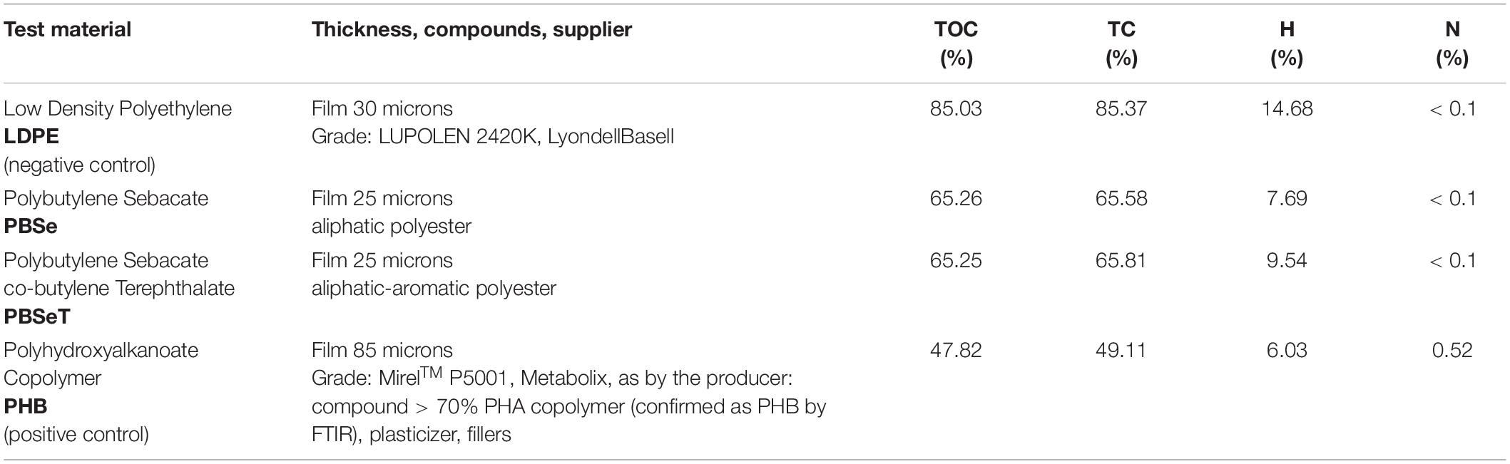
Table 1. List of tested polymers with their properties, film thickness, compounds, and supplier. Percentage of total organic carbon (TOC), total carbon (TC), hydrogen (H), and nitrogen (N) analyzed with standard methods.

The materials were tested as films, due to technical constraints in the processing only available with different thicknesses. The positive control PHB, marketed under the product name Mirel P5001 (Metabolix, United States) was described as “PHA copolymer” by the producer and the exact polymer was not disclosed. Our FTIR spectral analysis (data not shown) confirmed the materials as PHB. In the lab tests, small pieces of film (4 × 4, 2 × 4, 3 × 3, ø 2 cm) were directly incubated in the test vessels. For the mesocosm and field tests polymer film samples were mounted in HYDRA^® test frames (260 mm × 200 mm external and 200 mm × 160 mm internal dimensions leaving a surface of 320 cm² of material directly exposed), i.e., held between mesh (PET) and plastic frames (PE) (Supplementary Figure 1) to prevent mechanical impact on the sample, as described before (Lott et al., 2020).

Matrices Sediment and Seawater

Eulittoral sediment: Natural marine sediment for the eulittoral tests in the lab and in mesocosms was retrieved at about 0.1 m water depth from the beach of Fetovaia, Isola d’Elba, Italy, (42°44′00.1″N, 010°09′15.3″E) and is called “beach sediment.” Sublittoral sand: Carbonate sediment for the benthic mesocosm tests was collected by divers from the seafloor at 40 m depth off Isola di Pianosa, National Park Tuscan Archipelago, Italy (42°34′41.4″N, 010°06′30.6″E), and is called “seafloor sediment.” Larger pieces, like plant material, sea shells, pieces of driftwood, etc., were removed by sieving through a 10 mm mesh after collection. Seawater was taken at Seccheto, Isola d’Elba, Italy (42°44′06.5″N, 010°10′33.5″E) and was used for the lab experiments, to wash the sediments and to fill the mesocosms. The mesocosm tests were run twice for about 1 year each and specified as y1 and y2 in this text. The matrices were renewed after the first run and the physical and chemical properties of sand and water were analyzed with standard methods at the beginning of each experiment (for details see Lott et al., 2020). The water used in the mesocosm tests (see below) had low to moderate levels of organic carbon, nitrogen and phosphor compounds, and chlorophyll. No toxic substances such as heavy metals, organotin compounds, or persistent organic pollutants (POPs) were detected. The beach sand used for tests was in the grain size range of medium sand and of mainly siliclastic origin. The seafloor sediment used for the benthic experiments was mainly carbonate fine sand. Porosity and permeability were slightly lower for both sand types in y2 (Table 2). Metal concentrations were low or below the detection limit. The test for persistent organic pollutants (POPs) in the sediments used for the experiments was negative (details in Lott et al., 2020).

TABLE 2

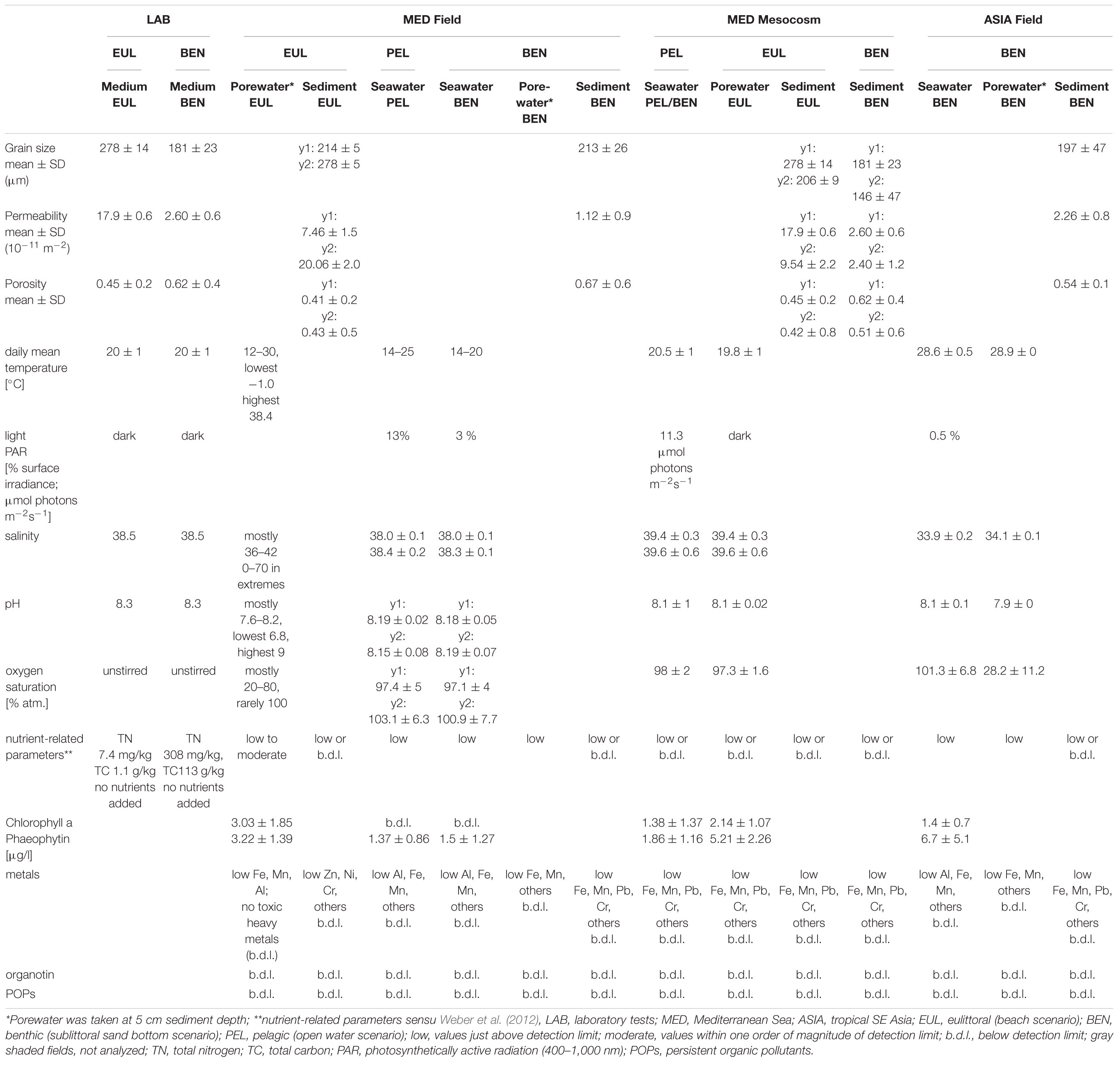
Table 2. Experimental conditions: Properties of the water and sediments from the lab, field, and mesocosm experiments.

Laboratory Tests

The lab tests were conducted at LeAF in Wageningen, Netherlands, with water and sediment from the Mediterranean field test locations (Table 2). The matrices were collected in plastic containers, shipped to LeAF and stored at 4°C until further use. At the start of the experiments, water and sediment were characterized with standard analytical methods.

Eulittoral Test (Beach Scenario)

The plastic samples were buried in 400 g of beach sediment under aerobic conditions as described in Tosin et al. (2012), following International Organization for Standardization (2019). The sediment had a water content of 18.9%, total solids content of 81.1%, of which volatile solids of 0.57%, total nitrogen of 7.4 mg/kg, and total carbon of 1.1 g/kg. No nutrients were added. The tests were carried out in 2-L Duran^® wide-mouth bottles and a container for the CO₂ sorption connected to a side port. The container was filled with 30 mL of 0.5N KOH solution. The bottle and the container were closed with a Python rubber stopper (Rubber BV, Hilversum, Netherlands). The bottles were incubated in the dark in a closed box that was placed in a temperature-controlled room (20 ± 1°C). The test materials (PBSe and PBSeT) were square-shaped specimens with a dimension of approximately 40 mm × 40 mm. The negative control was done with 40 mm × 40 mm specimens of LDPE. For the test with PHB as the positive control specimens were cut in 20 mm × 40 mm pieces (because of the high grammage). The mass of each specimen (about 100 mg) was recorded. For the test 15 reactors were prepared to enable testing in triplicates of PBSe, PBSeT, PHB (reference material/positive control), LDPE (negative control), and blanks to correct for endogenous respiration. All reactors were pre-incubated without plastic samples to assess the endogenous respiration. After 1 week of pre-incubation, the CO₂ production was measured. The results showed that the endogenous respiration was similar in the bottles. After the pre-incubation, the test was started. For this, the reactors were opened and 100 g of sediment was removed. The sediment surface was smoothened and two specimens of test materials PBSe or PBSeT or LDPE or one specimen of PHB was placed on the surface. Thereafter the withdrawn sediment was carefully put on top of the sediment and test material. The specimens were covered with sand in a homogenous layer. The blanks for endogenous respiration did not receive any test specimen.

The extent of biodegradation [i.e., (endogenous) respiration] was assessed by determining the amount of carbon dioxide produced and absorbed in the KOH solution by titration with 0.3N HCl solution to pH 8 and thereafter further to pH 3.8. The amount of CO₂ absorbed was calculated according to the formula given by Tosin et al. (2012). The container for the CO₂ absorber was removed and analyzed and titrated before its capacity was exceeded. Each time the KOH was replaced by a fresh solution the reactor was weighed to monitor moisture loss from the sediment and allowed to sit open for approximately 15 min so that the air in the reactor was refreshed before resealing the reactor. Distilled water was added back periodically to the sediment to maintain the initial weight of the reactor. The tests were terminated after 331 days.

Benthic Test (Seafloor Scenario)

The biodegradation under aerobic conditions at the water-sediment interface was tested following Tosin et al. (2012) and International Organization for Standardization (2016). At the start of the experiments, the medium used for the benthic lab test had a pH of 8.3, a water content of 95.8%, a total solids content of 4.2%, of which volatile solids were 15.7%. The tests were carried out in 250 ml Erlenmeyer flasks with a container attached to a side port filled with 3 mL 0.5 N KOH for CO₂ absorption. The bottle and the container were closed with a Python rubber stopper (Rubber BV, Hilversum, Netherlands). The bottles were incubated in the dark in a closed box that was placed in a temperature-controlled room (20 ± 1°C). The test materials (PBSe and PBSeT) were square-shaped specimens with a dimension of approximately 30 mm × 30 mm. The negative control was done with a specimen of LDPE. For the test with PHB as the positive control specimens were cut in circles of 20 mm diameter. The mass of each specimen (about 36 mg for PHB, about 25 mg for the others) was recorded. For the test 15 reactors were prepared to enable testing in triplicates of PBSe, PBSeT, PHB [reference material/positive control, LDPE (negative control)], and a blank without test material to correct for endogenous respiration. Sediment (30 g) was placed at the bottom of each reactor with 70 ml seawater and 3 ml of 0.5N KOH (the CO₂ absorbing solution) was introduced in the container. Endogenous respiration was measured after 1 week by measuring the CO₂ production. The results showed that the endogenous respiration was similar in the bottles. After the initial week of pre-incubation, the test was started. For this, the reactors were opened and the specimen of test materials PBSe or PBSeT or LDPE or PHB were placed on top of the sediment. About 25–35 mg of test material or LDPE or PHB was introduced in the reactors. The blanks for endogenous respiration did not receive any test specimen. The carbon dioxide produced in each reactor reacted with KOH and was titrated as described above. The tests were run for 331 days. The content of the test bottles was sacrificed for the retrieval of remaining plastic test items after the termination of the test.

Modeling the Half-Life t_0.5 of Biodegradation

For all statistical analyses, R project was used (R Core Team, 2020). From the raw data of CO₂ release over time (equaling aerobic biodegradation) the half-life of the polymer was analyzed using Three Parameter Logistic Regression (3PL) by fitting the data with a non-linear model (package nlme) to the formula:

$y\left(t\right)=y_{max}+\frac{-y_{max}}{1+{(\frac{t}{c})}^b}(1)$

where y is the polymer biodegradation in percent, t the corresponding time in days, and y_max, b, and c the curve parameters estimated by the model and representing the biodegradation at the plateau, the slope-factor and the inflection-point of the curve, respectively (adapted from Junker et al., 2016). Since the same test flask was measured repeatedly over time, the data is not independent. However, independence of the observations is an important assumption for this statistical analysis. Therefore, the replicate ID was included as a random factor, which allowed different estimated values for y_max for each flask. If no model parameters could be estimated, y_max was below 0 (as for LDPE), and/or estimated parameters (except y₀) were not significantly different to 0 no biodegradation was assumed. To visualize the confidence interval (CI) of the predicted disintegration curves, a Monte Carlo simulation approach was employed to re-sample for each x value (days) 50,000 predicted values (% biodegradation) considering the estimates and variance of model parameters. The range of the 95% percentile of these samples was considered as 95% confidence interval. Before calculating the half-life, it had to be tested if y_max was higher than 50 %. Therefore, empirical p-values were used. 500,000 values for y_max were re-sampled considering the coefficients predicted by the non-linear model and its variance. If less than 5% of these values were below 50%, the plateau was assumed to be greater than or equal to 50%. If this condition was fulfilled, 500,000 values for the half-life (t_0.5) were generated by setting y in the 3PL equation to 50%, using the estimated values and corresponding variances of the model parameters, and solving the formula to t. In some cases, the half-life could not be calculated as described because y_max assumed values were below 50% (however, in less than 5% of the cases, as shown by the previous test). In these cases, the half-life was set to infinity. To compare calculated values for t_0.5 between habitats and experiments, the difference between two groups of t_0.5 values was calculated. For these pairwise comparisons, empirical p-values were calculated by $p=\frac{2r}{n}$, where r is the number of t_0.5 differences either above or below zero and n the number of trails (i.e., 500,000). If all r values were below or above 0, the lowest possible value for p was assumed (2⋅1/n = 4⋅10^–6). p-values were adjusted for multiple comparisons using the Holm method (Holm, 1979). The distributions of the re-sampled half-life values were visualized by violin plots in which the spread along the x axis represents the frequency of values on the y axis (half-life). Different letters indicate significantly different groups.

Mesocosm Tests

The mesocosm tests were conducted in two consecutive years (y1 and y2) in triplicates in a climate chamber as described before (Lott et al., 2020). Three coastal habitats were simulated in a tank system consisting of two 630-L plastic containers placed on top of each other. The upper tank contained a layer of siliclastic beach sediment in which the samples were buried (eulittoral scenario) and which was flooded with seawater every 12 h. The bottom of the upper tank was perforated to allow the water to slowly drain to the lower tank, thus mimicking a 12-h tidal cycle at the samples. The lower tank contained a layer of carbonate seafloor sediment on which samples for the benthic test were placed. The pelagic test was performed by hanging samples in the water column of the lower tank, which was illuminated on a 12:12 h rhythm. The bulk water of the two tanks was connected by pipes and constantly moved by additional pumps in the lower tank. The water was regularly checked for salinity, pH, and oxygen saturation and compensated for evaporation loss by adding demineralized water if necessary. The temperature was 20.5°C ± 1°C and mean light intensity on the sediment surface of the benthic tests was 11.56 μmol photons⋅m^–2⋅s^–1. Salinity was 39 ± 1. The pH was 8.1 ± 0.1. The oxygen concentration was close to air saturation (98 ± 2%). In the first year (y1), three polymers were tested in the mesocosm experiments: LDPE, PHB, and PBSeT were sampled at four time points (t1–t4) (Supplementary Table 1). In the second year (y2), PBSe was tested additionally and sampled at two time points (t1 and t3). Three to five samples were retrieved ca. every 2.5 months from the tanks. The last sampling interval of the y2 experiment was only 1.5 months.

Field Tests

Field tests were performed in the eulittoral (beach scenario), the pelagic (open water scenario), and the benthic (sublittoral seafloor) (Figure 1) as described before (Lott et al., 2020).

FIGURE 1

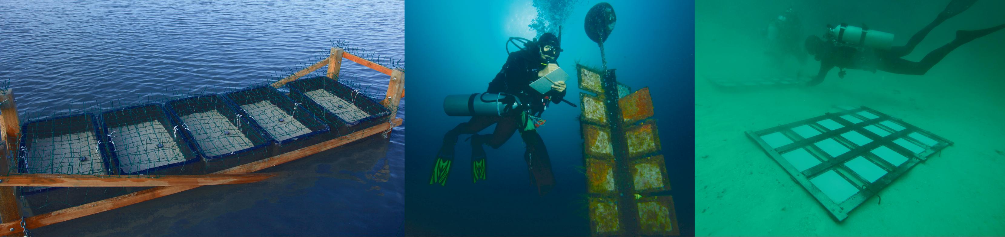
Figure 1. Field test systems: left: eulittoral test: Samples were exposed in bins filled with beach sand on a rack in the midwater line, center: pelagic tests: samples attached to a floating rack exposed at 20 m water depth, right: benthic tests: samples were mounted in panels that were fixed on the sandy seafloor at 40 m (Mediterranean Sea) and 32 m water depth (SE Asia).

For environmental conditions at each site see Table 2. For sampling dates and intervals see Supplementary Table 2.

Eulittoral Tests

The eulittoral tests were set up on the Island of Elba, Terme di San Giovanni, Portoferraio (N 42°48′12.1″N, 010°19′01.0″E, Italy in a former saline basin, now open to the sea (Lott et al., 2020). The test system consisted of 60-L plastic bins filled with beach sediment in which the samples were buried. To simulate an intertidal sandy beach the bins were placed on wooden racks in the midwater line in a way that the samples were exposed to changing conditions of being wetted and falling dry with the tides.

Pelagic and Benthic Tests

The pelagic and benthic field tests in the Mediterranean Sea were performed in the marine protected area of the National Park Tuscan Archipelago off the Island of Pianosa (42°34′41.4″N, 010°06′30.6″E), Italy. The benthic field tests in South-East Asia were performed in Sahaong Bay (01°44′35.4″N, 125°09′09.3″E), Pulau Bangka, NE Sulawesi, Indonesia. For details see Lott et al. (2020).

The pelagic test systems consisted of a rack to which the sample frames were attached, anchored to stay afloat at a water depth of 20 m, chosen to avoid influence by surface wave activity. For the benthic tests, the samples were mounted to a flat panel which was fixed to the seafloor at 40 m in the Mediterranean Sea and to 32 m in Indonesia. These depths were chosen to avoid interference of the experiments with the seagrass meadows or coral reef structures, respectively.

In the Mediterranean field tests, in the first run of field experiments (y1) in all three habitats five replicates of PHB, PBSeT, and LDPE were exposed and sampled about every 2.5 months. One additional set was left exposed for 2 years (t₅), together with new samples for a second 1-year run (Supplementary Table 2). From these additional sets, two replicates were sampled from the pelagic and benthic experiment after 678 days and five replicates were sampled from the eulittoral test system after 686 days. In the second experiment run (y2), the number of replicates per time was reduced to three. Also, PBSe was added as test material with three replicates in the pelagic and benthic tests, and two replicates per time in the eulittoral test. The data from y1 and y2 were pooled in the analysis as experiment y1 followed the same seasonality as y2.

In the wet tropics of South-East Asia, tests were conducted in 2017 and 2018. Three replicates of PHB, PBSe, and PBSeT were exposed to the benthic habitat. Sampling occurred after 19, 48, 62, 90, and 310 days for PHB, after 16, 90, 130, and 310 days for PBSe and after 90 and 310 days for PBSeT.

Sampling and Data Acquisition From Mesocosm and Field Tests

At the given time interval, the sample frames were carefully detached from their racks (pelagic, benthic) or dug out of the sediment (eulittoral), rinsed in ambient water, packed singly in plastic (PE) bags covered with water, and brought to the laboratory for further treatment the same day. Each frame was opened and the sample photographed in a standardized way. Then the samples were washed in freshwater and left to dry at room temperature overnight.

Disintegration Measurements

In the open-system tests of the mesocosm and field experiments, material disintegration was determined as a proxy for biodegradation assuming that the samples were protected from mere physical damage well enough by the construction of the test frame. The degree of disintegration (% area loss) of each sample was determined photogrammetrically. Dried samples (Mediterranean tests) were scanned on a LIDE 210 flatbed scanner (Canon Inc.). For the Indonesian samples, photos (Canon EOS 5D MkII) of the freshly sampled films were used and analyzed for the proportion of lost vs. still intact surface using the software ImageJ¹.

Calculating Half-Life t_0.5 Based on Disintegration Data

The data from the field and mesocosm experiments was analyzed in a different way than described for the lab test. Far fewer data points were acquired in the field and mesocosm tests than in the lab experiment, therefore we chose a linear model with less degrees of freedom (i.e., estimated parameters) over the non-linear logistic regression used to analyse the lab data. The disintegration of the polymer area over time was analyzed using beta regression (package betareg) because response values consisted of percent data. The extreme values of 0% and 100%, were transformed according to Smithson and Verkuilen (2006). At the start of the experiment (t = 0 days), no disintegration was assumed, therefore n artificial values with 0% disintegrated area were included, where n is the number of replicates in the data-subset. For each habitat and experiment (field vs. mesocosm) one model was applied. For the mesocosm experiment, additionally, the influence of the year of the experiment was analyzed and integrated into further analysis if a significant interaction with the variable time existed. Different models were applied using logit, cloglog, cauchit, and loglog link-functions (see Supplementary Table 3). The best model was then selected by comparing the Root Mean Square Deviation (package caret). When comparing the disintegration rate between habitats it is not sufficient to only compare the slopes. The non-linear shape of the back-transformed disintegration curve depends on both, the y-intercept a and the slope b. Therefore, rather half-life (t_0.5) should be compared. Since different link-functions were used, different formulas had to be applied to calculate the corresponding x (time) values at which the disintegration reached 50 %. For example, in the case of logit-transformed data, 50 % of the material is left at the x-intercept of the regression curve for transformed data:

$\text{logit}\left(50\%\right)=\log \left(\frac{p}{1-p}\right)=\text{log}\left(\frac{0.5}{1-0.5}\right)=0(2)$

The x-intercept can be calculated by $t=\frac{-a}{b}$. The formulas used for the other link-functions are compiled in Supplementary Table 3. A Monte Carlo simulation approach was applied to re-sample 500,000 values for a and b considering model parameter estimates and variance and a normal distribution. The comparison of the generated half-life was performed with empirical p-values as described for the lab experiment.

Results

Laboratory Tests With Mediterranean Sea Matrices

The lab tests with matrices from two of the shallow water habitats chosen for field and mesocosm tests were done to prove the biodegradability of the three tested polymers PHB, PBSe, and PBSeT under optimized lab conditions with natural matrices. The eulittoral test (beach scenario) and the benthic test (seafloor scenario) were selected because the tested polymers have a higher specific density than seawater and will sink to the seafloor. The pelagic test was not performed due to space limitations in the laboratory. The biodegradation in both habitats was fastest for PHB and similar for PBSeT and PBSe (Figure 2).

FIGURE 2

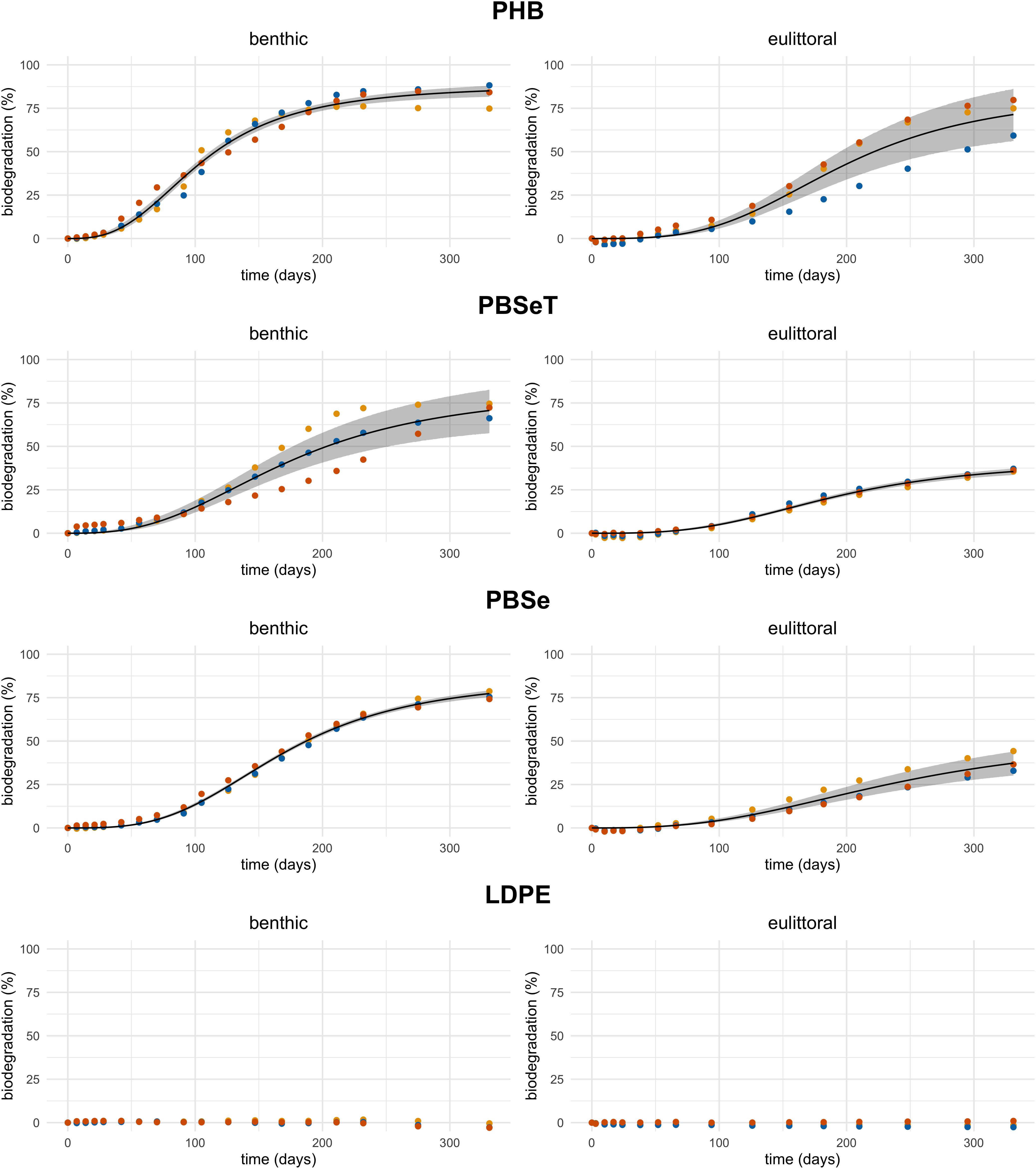
Figure 2. Laboratory experiments with Mediterranean Sea water and sediment: Biodegradation curves of PHB, PBSe, and PBSeT when incubated with seafloor sediment at the sediment-seawater interface (benthic) and buried in beach sand (eulittoral). Colors red, yellow, and blue indicate samples from different test flasks, dots represent raw data analyzed in the model. The model curve ± 95% CI (shaded area) was drawn if estimated parameters were significantly different from 0.

In the benthic test, a plateau was reached or nearly reached after about 1 year for the three test materials. PHB was more or less completely converted to CO₂ as is evidenced by the 81% biodegradation that was calculated from the CO₂ production. The biodegradation percentage of PBSe and PBST was 71 and 76%, respectively, which also indicates that mineralization of these test items was almost complete, given that an incorporation of about 25–30% of substrate carbon into microbial biomass is assumed [see e.g., Payne (1970) for conversion rates in bacterial cultures]. Except for LDPE none of the plastic test items could be retrieved, not even in fragments, from the benthic test bottles which indicates that the disintegration of the test items was complete. In some cases, e.g., for PBSe very small particles were visible but these were in the size range of sand grains. LDPE was recovered intact from the flasks and biodegradation was not detected. In the eulittoral test, none of the three materials reached the plateau phase within the duration of the experiment (331 days). PHB was completely disintegrated in all flasks. For both, PBSe and PBSeT, one of the three replicates could be retrieved degraded to 25 and 33%, respectively.

The respective half-lives t_0.5 predicted by the model are given in the following text without the confidence intervals which can be found as a summary in Table 3 at the end of the results section. For PHB in the benthic test, the half-life was 116 days and significantly (p < 0.001) lower than in the eulittoral test (222 days, Figure 3). For PBSe, the modeled t_0.5 was 203 days and for PBSeT 187 days both in the benthic test. In the eulittoral test, the exposure time for both materials was not sufficient to reach a biodegradation of more than 50%, therefore modeling t_0.5 was not possible.

TABLE 3

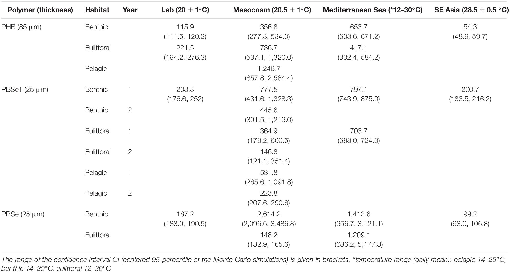
Table 3. Summary of all tests: Half-lives t_0.5 of PHB, PBSe, and PBSeT as predicted by statistical modeling of the experimental data.

FIGURE 3

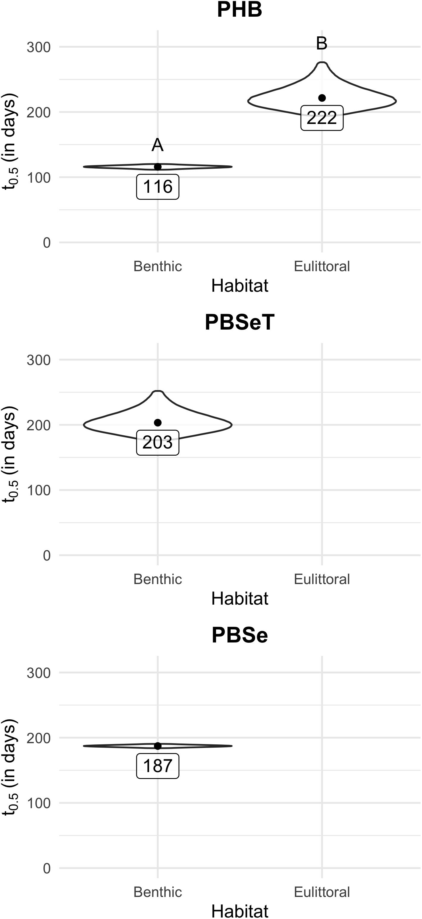
Figure 3. Laboratory experiments with Mediterranean Sea water and sediment: Biodegradation half-lives t_0.5 of PHB, PBSe, and PBSeT. Monte Carlo simulations of half-life for tested polymers in two habitats, on the seafloor at the sediment-seawater interface (benthic) and the beach scenario (eulittoral). Shown is the distribution of the centered 95 percentiles of the simulations as violin plots. The dot in the center of each violin represents the half-life as calculated from the estimated model coefficients; the value is given in the box below. Letters above the violin plot represent the results of the multiple comparisons. Different letters (A, B) indicate significantly different groups (i.e., Holm-adjusted p-value below α = 0.05). For PBSeT and PBSe in the eulittoral habitat, no half-life could be calculated because the plateau phase was not reached and values remained below 50 % (cf. Figure 2).

Mesocosm Tests With Mediterranean Sea Matrices

All test materials, except LDPE, showed disintegration with high heterogeneity between replicates, habitats, and material type. About 90% disintegration was observed for PBSe and PBSeT in the eulittoral test in y2 after 238 days (Figure 4) and for PBSeT in the pelagic test in y2 after 271 days. Most samples of PBSe and PBSeT in the other habitats were disintegrated less than 50% after 308 and 270 days of exposure, respectively.

FIGURE 4

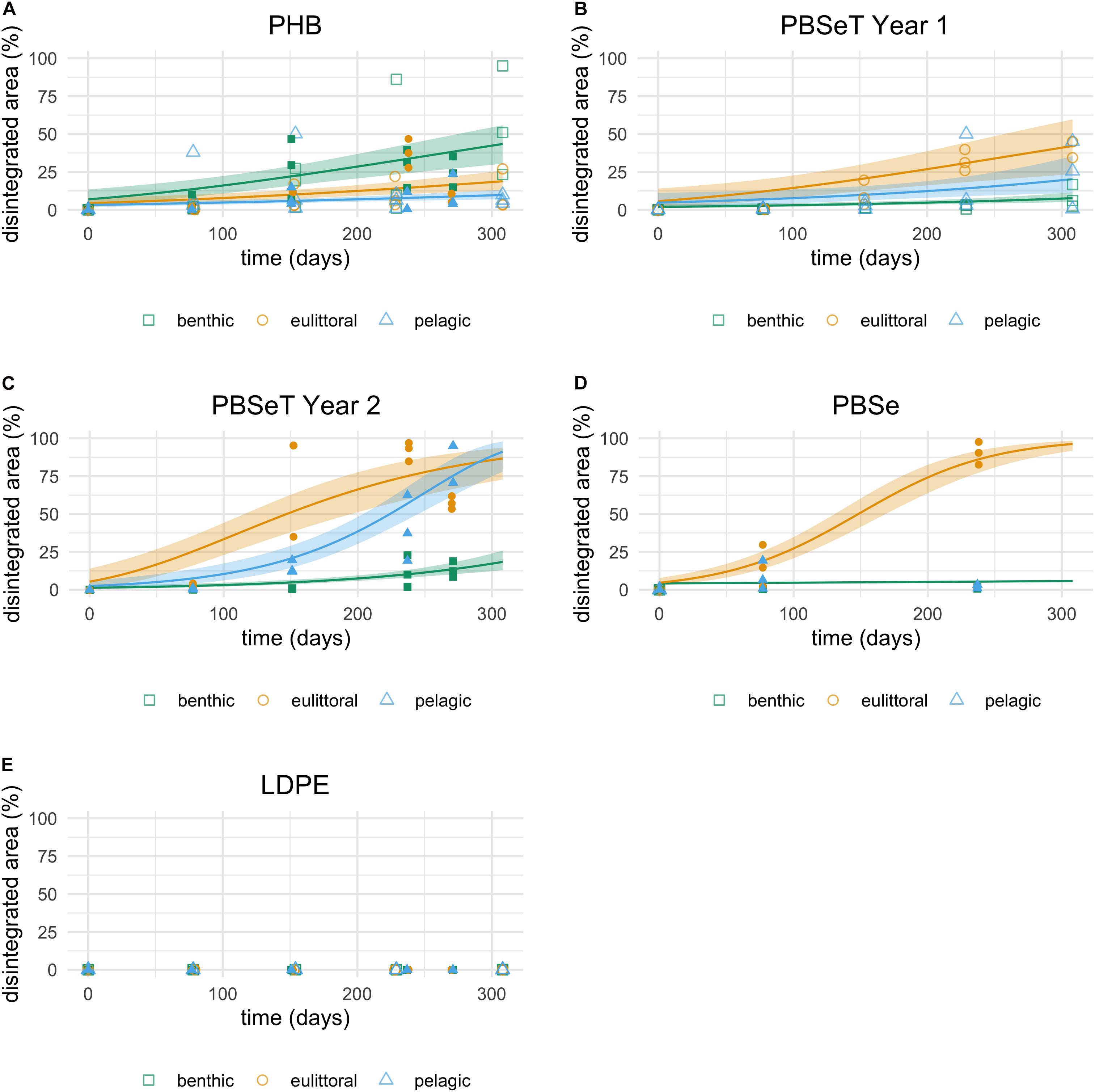
Figure 4. Mesocosm experiments with Mediterranean Sea water and sediment: Disintegration curves of (A) PHB, (B) PBSeT, and (C) PBSe over 10 (year 1) and (D) 9 (year 2) months when exposed in the seafloor scenario at the sediment-seawater interface (benthic), in the water column (pelagic) scenario or buried in the intertidal sandy beach (eulittoral) scenario. (E) For LDPE no disintegration was measured. The model curve ± SE (shaded area) was drawn if the slope was different from zero and positive. Dots represent raw data analyzed in the model (open = year 1, filled = year 2), For PBSeT two significantly different model curves are shown. Colors represent the habitat (green = benthic, orange = eulittoral, blue = pelagic).

The half-life of PHB did not differ between the two experiments (year 1 and year 2) within each habitat. The predicted half-life in the benthic habitat (357 days) was significantly lower than in the eulittoral (737 days) and pelagic (1,247 days) habitats (Figure 5, Table 3, and Supplementary Table 4). PBSeT had a t_0.5 of 778 days in y1 and 446 days in y2 in the benthic tests, 365 days in y1 and 147 days in y2 in the eulittoral tests, and 532 days in y1 and 224 days in y2 in the pelagic tests (Figure 5 and Table 3). In the eulittoral experiment, the degradation was significantly faster in the second-year experiment than in the first-year experiment (p = 0.0071). No significant differences were detected between both experiments (y1 and y2) in the benthic and pelagic tests (Supplementary Table 5). The half-life of PBSe was significantly higher in the benthic tests (2,614 days) than in the eulittoral test (148 days, p < 0.0001, Figure 5, and Table 3). Predictions for the half-life of PBSe in the benthic test should be considered with caution, since maximum degradation after 237 days was 1.5%, making predictions of the time needed until 50% is degraded unreliable. In the pelagic test, no significant disintegration was measured for PBSe. For LDPE no disintegration at all was measured in any test during the exposure time thus it was not possible to model t_0.5.

FIGURE 5

Figure 5. Mesocosm experiments with Mediterranean Sea water and sediment: Disintegration half-lives t_0.5 of PHB, PBSeT, and PBS. Monte Carlo simulations of half-life for tested polymers in three habitats (on the seafloor at the sediment-seawater interface (benthic), the beach (eulittoral), and the water column (pelagic) scenario). Shown is the distribution of the centered 95 percentiles of the simulations as violin plots. The dot in the center of each violin plot represents the half-life as calculated from the model coefficients, and the value is given in the box below. Letters above the violin plot represent the results of the multiple comparisons. Different letters indicate significantly different groups.

Field Tests

Mediterranean Sea

All test materials, except LDPE, showed signs of disintegration when in contact with sediment, i.e., in eulittoral and benthic tests (Figure 6). In the pelagic tests, no disintegration was observed for PHB and PBSe within 2 years. For PBSeT, material disintegration increased significantly over time, but at a very low slope. The maximum disintegration after 676 days was only 1.01% and 0.13%, therefore we did not predict the half-life. The heterogeneity between replicates was high. The half-life t_0.5 of PHB in the benthic test (654 days) was significantly higher (p = 0.0161) than in eulittoral test (417 days, Figure 7, Table 3, and Supplementary Table 6). In the pelagic test, modeling of t_0.5 was not possible because no disintegration was measured during the exposure time. PBSeT had a t_0.5 of 797 days in the benthic test, which was significantly lower than in the eulittoral test (704 days, Figure 7, Table 3, and Supplementary Table 7). PBSe had a t_0.5 of 1,413 days in the benthic test and of 1,209 days in the eulittoral test (Figure 7, Table 3, and Supplementary Table 8).

FIGURE 6

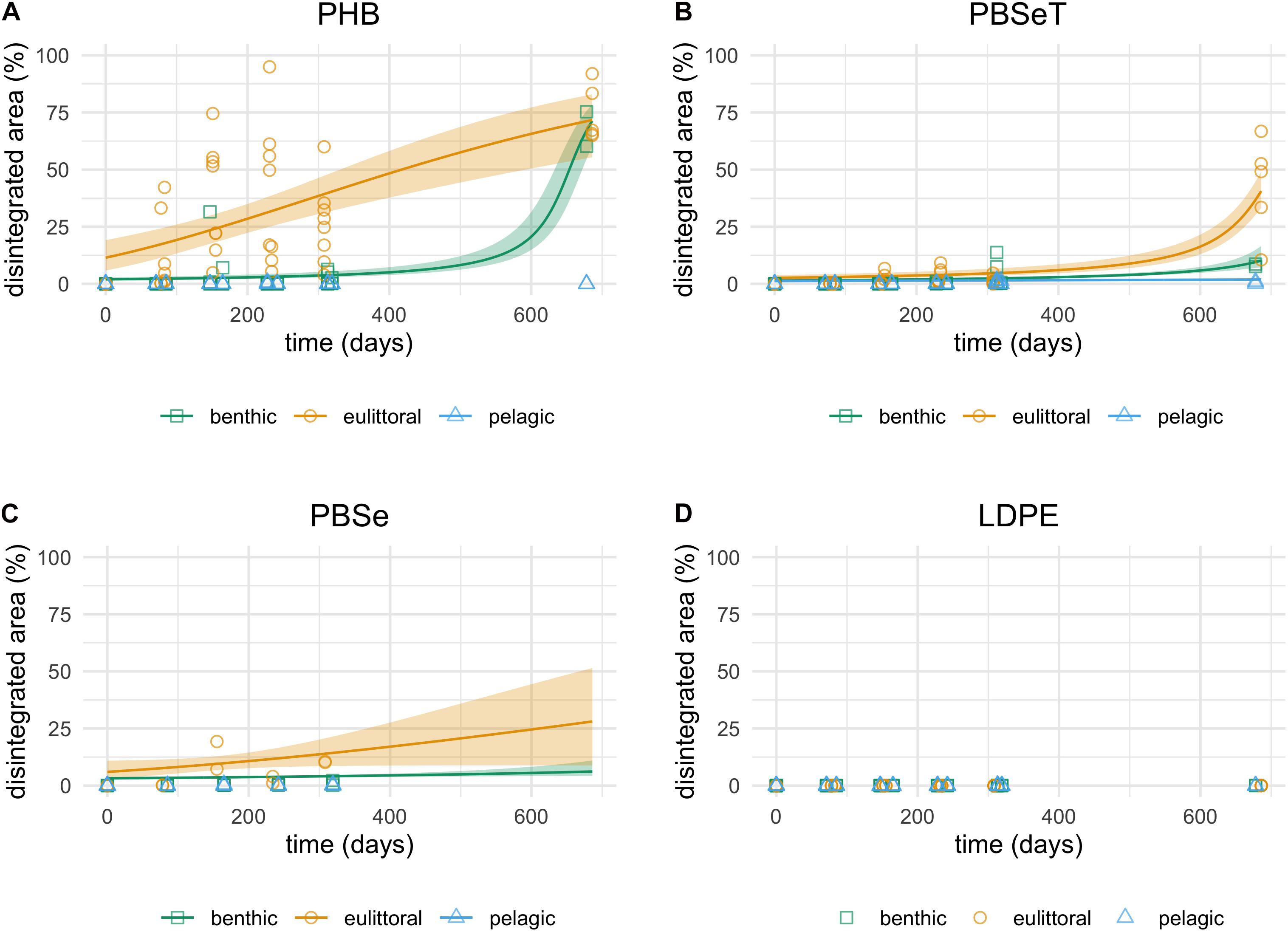
Figure 6. Field experiments in the Mediterranean Sea: disintegration curves of (A) PHB, (B) PBSeT, and (C) PBSe when exposed on the seafloor at the sediment-seawater interface (benthic), the beach (eulittoral) and the water column (pelagic) scenario. (D) For LDPE no disintegration was measured. The model curve ± SE (shaded area) was drawn if the slope was different to zero and positive. Dots represent raw data analyzed in the model. Colors represent the habitat (green = benthic, orange = eulittoral, blue = pelagic).

FIGURE 7

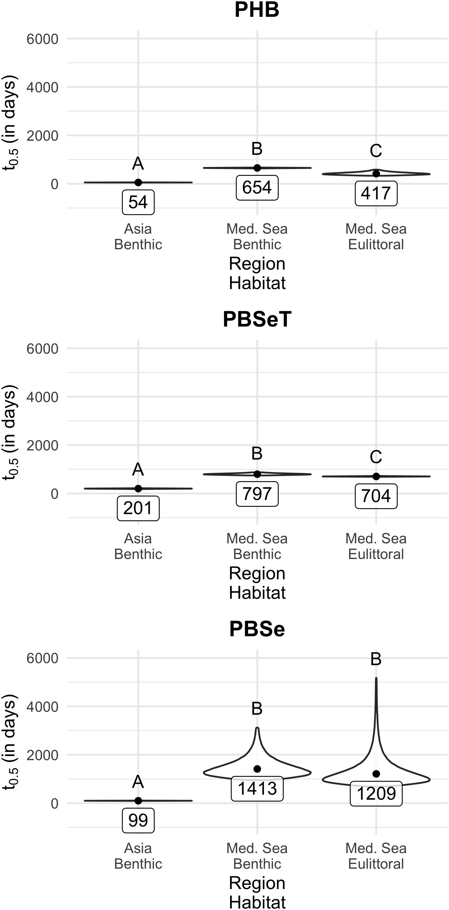
Figure 7. Comparison of the disintegration half-lives t_0.5 of PHB, PBSeT, and PBSe from field experiments in tropical SE Asia and the Mediterranean Sea: Monte Carlo simulations of half-life for tested polymers in the benthic (seafloor sediment-seawater interface) in Asia and the Mediterranean Sea and in the eulittoral (beach scenario) in the Mediterranean Sea. Shown is the distribution of the centered 95 percentiles of the simulations as violin plots. The dot in the center of each violin plot represents the half-life as calculated from the model coefficient and its value is given in the box below. Letters above the violin plot represent the results of the multiple comparisons. Different letters indicate significantly different groups (i.e., Holm-adjusted p-value below α = 0.05).

SE Asia

All test materials, except LDPE, fully disintegrated in the benthic test within few months (Figure 8) with heterogeneity between replicates. The t_0.5 for PHB was 54 days, for PBSeT 201 days, and for PBSe 99 days (Figure 7 and Table 3). The disintegration of all polymer types was significantly faster in SE Asia compared to the Mediterranean Sea (Figure 7 and Supplementary Tables 6–8).

FIGURE 8

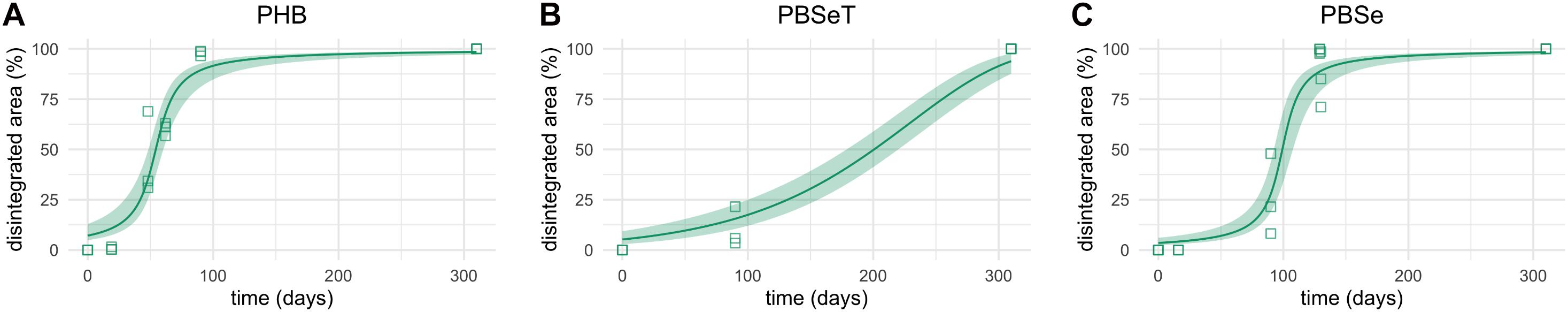
Figure 8. Field experiments in tropical SE-Asia: Disintegration curves of (A) PHB, (B) PBSeT, and (C) PBSe exposed on the seafloor sediment-seawater interface (benthic) for almost one year (310 d). The model curve ± 95% CI (shaded area) was drawn if the slope was different from zero and positive. Squares represent raw data analyzed.

Summarized (Table 3), in the field tests in the Mediterranean Sea, the t_0.5 of a 25 μm thick film of PBSeT and PBSe and an 85 μm thick film of PHB ranged between 1.8–3.9 years in the benthic tests (seafloor scenario) and 1.1–3.3 years in the eulittoral tests (beach scenario). No significant disintegration occurred for any of the materials in the pelagic tests (water column scenario). In the benthic test in SE Asia, t_0.5 was about 0.15 years (2 months) for PHB, 0.55 years (7 months) for PBSeT, and 0.27 years (4 months) for PBSe. For LDPE no disintegration was measured, thus no half-life was possible to calculate.

Discussion

The aim of this study was to prove the biodegradability of biodegradable polymers under laboratory conditions, to test the biodegradation performance under natural field conditions, and in a tank test system with natural matrices.

We tested the performance of PHB (as reference material and positive control), PBSe, and PBSeT in three different habitat scenarios, namely the intertidal sandy beach (eulittoral), the sandy sublittoral seafloor (benthic), and the open water column (pelagic) in a three-tier test approach in closed-vessel laboratory, in mesocosm tank and in-situ field tests, some of which in two different climate zones (the warm-temperate Mediterranean Sea and the tropical sea of SE Asia).

Furthermore, we introduced an analytical tool based on statistical modeling to predict the specific half-life calculated from the experimental data for each set of test conditions, to use the half-lives to numerically compare the performance of three different materials tested, and to numerically compare the performance of one material in different environmental settings.

The three-tier approach to test the performance of biodegradable plastic in the marine environment gave a comprehensive view and could differentiate between sediment type, habitat, and climate zone.

Half-lives t_0.5 Differed Between the Materials in All Test Systems and Habitats

Laboratory Experiments

In the lab tests, biodegradation of PHB was faster in the benthic than in the eulittoral test and similar to the results obtained by Briassoulis et al. (2020) in a comparable setting. For PBSe and PBSeT in the eulittoral tests the plateau phase of biodegradation, as calculated by CO₂ evolution, was not reached within the test period and values remained below 50 %. Consequently, t_0.5 could not be calculated. The leveling out of the biodegradation curves in the benthic test (Figure 2) indicates a limitation of substrate for the bacteria and the nearly complete conversion of the polymer into CO₂ and microbial biomass. In the humid sand of the eulittoral tests, the CO₂ production rate was generally lower than at the submersed sand surface in the benthic test. However, the fact that in most of the experiments no or only little test material was left could indicate a more efficient build-up of microbial biomass in the eulittoral, a (yet) incomplete mineralization of soluble intermediates of biodegradation, a limitation of nutrients or inhibition by a hypothetical starvation factor as proposed by Mistriotis et al. (2019) in soil.

For PHB, both lab tests applied showed the biodegradability of the positive control but also revealed significant differences in the performance under the different experimental conditions of a simulated seafloor (benthic) and a simulated beach (eulittoral). The lab tests were conducted under static conditions without stirring or shaking the medium leaving the system purely diffusion-driven. It can be assumed that oxygen availability to the acting microbes was most of the time limited. This is also corroborated by the observation of black spots on the sediment below some of the samples in the benthic test indicating the precipitation of dark metal salts under anoxic conditions. As the methods for both tests are defined as aerobic (Tosin et al., 2012; International Organization for Standardization, 2019; International Organization for Standardization, 2016) some technical modifications as e.g., gentle stirring as proposed by Briassoulis et al. (2020) could be considered to assure the medium is well oxygenated.

Although both tests worked well it is recommended to use the test scenario that is most environmentally relevant for the purpose and to choose well the matrices, especially the sediment used. Sediments of different origin and quality most likely will differ in their microbial activity.

Mesocosm Experiments

The testing of the biodegradation of plastic in mesocosms of a larger volume was demonstrated as a viable complement or even alternative to field tests and allowed tests with natural matrices without access to running seawater (Lott et al., 2020). The t_0.5 of the three polymers modeled from disintegration measurements in the open system tests in mesocosms (Figure 5) were about two to four times higher (excluding PBSe, see below) than the ones calculated from the CO₂ evolution in the lab tests (Figure 3) with the same temperature applied, which confirms the laboratory tests as optimized compared to field tests (even though oxygen availability might have been varying). This fact also confirms our assumption that using the degree of disintegration of samples that are well protected from physical impact as a proxy for biodegradation is well suited to measure the biological processes at the material in the open systems of mesocosms and field experiments rather than a mere physical deterioration of the plastic.

In the mesocosm tests, the variability in the degree of disintegration of single specimens was high even within one tank system, but also between the three replicate tanks and between years, reflected in the sometimes wide 95% confidence intervals (CI) (Figure 4) as a common feature of all tests. This is attributed to the patchiness of the microbial community, also known from natural sediment environments (e.g., Böer et al., 2009). As can be seen from the shape of the violin plots, the variability within one test is higher in most of the scenarios where degradation was slower, thus half-life higher. For most tests, we applied a set of triplicates for each sampling interval which was just sufficient to obtain a statistically significant basis for modeling. However, this is the absolute minimal replication. Leaving a part of the samples longer deployed in the field tests than planned, led to an insufficient replication, especially considering the high variability observed in all tests. We therefore recommend using 4 or 5 replicates per interval to balance for variability. Furthermore, as seen when comparing the predictions from Asia and the Mediterranean Sea, the estimation of half-life is more precise when higher disintegration (at least about 75%) is reached.

Although observationally different, half-lives were not significantly different between the benthic and eulittoral habitat for the positive control PHB. Also for PBSeT, no consistent significant differences could be found for the half-lives between habitats. Only in the eulittoral test, the half-life in year 2 was significantly lower than in year 1. PBSe showed significantly different half-lives in the benthic and the eulittoral tests. However, very low values for the maximum disintegration in the benthic habitat (1.7% after 237 days) make the prediction of the half-life for this treatment unprecise and the t_0.5 predicted by the model should be taken rather as a rough indication and interpreted with caution. Comparing the performance of the three biodegradable materials in the different mesocosm tests the positive control PHB did disintegrate fastest in the benthic habitat whereas PBSe and PBSeT disintegrated fastest in the eulittoral habitat.

Field Tests

The half-lives in the Mediterranean field tests were higher than in the lab for the benthic test for all three polymers, about six times for PHB and about four and eight times higher for PBSe and PBSeT in the eulittoral, respectively. The field test in the Mediterranean Sea revealed significant differences between habitats and, compared with the tests in SE Asia, between climate zones. For all three biodegradable polymers PHB, PBSe, and PBSeT, disintegration was faster in the eulittoral than in the benthic. No significant disintegration was observed in the ultraoligotrophic setting of the Mediterranean pelagic. In the open water of the pelagic, the abundance of microbes is several magnitudes less (e.g., Schmidt et al., 1998) than in seafloor sediments, thus the overall activity of the microbial community is considered much lower. In the tropical waters of SE Asia, disintegration in the benthic was four to fourteen times faster than in the tests in the Mediterranean at the Island of Pianosa.

Marine (and aquatic) biodegradation tests in general often use water as the only matrix (e.g., ASTM, 2017) and give low rates as results (e.g., Bagheri et al., 2017). For biodegradable plastics, we consider this test scenario as the least environmentally relevant given that most biodegradable polymers have a density higher than water and will sink (or float at the water surface if the bulk density of a plastic object (e.g., a closed bottle or foamed material) is <1). However, a water column test is motivated for plastic items typically applied in the open water such as in aquaculture or fisheries.

Temperature Differences Explain Well Different Biodegradation Rates

Temperature is considered one of the most important environmental factors influencing the biodegradation rate. Pischedda et al. (2019) found a significant exponential relation between temperature and the biodegradation rate of a biodegradable plastic material in lab experiments with soil, in accordance with the Arrhenius equation, with the limitation of only three data points and thus no degree of freedom. For a rough estimation of the relationship between biodegradation rate and temperature in our experiments, we therefore applied an exponential model (Figure 9), confirming a significant negative relationship [F(1, 8) = 17.654, p < 0.003] between the predicted half-life and the average temperature in the mesocosm and field tests (Asia = 28.5°C, Mediterranean = 17.5°C, Mesocosm = 20.5°C). To increase datapoints to a more reasonable number, we did not differentiate between the different polymer types.

FIGURE 9

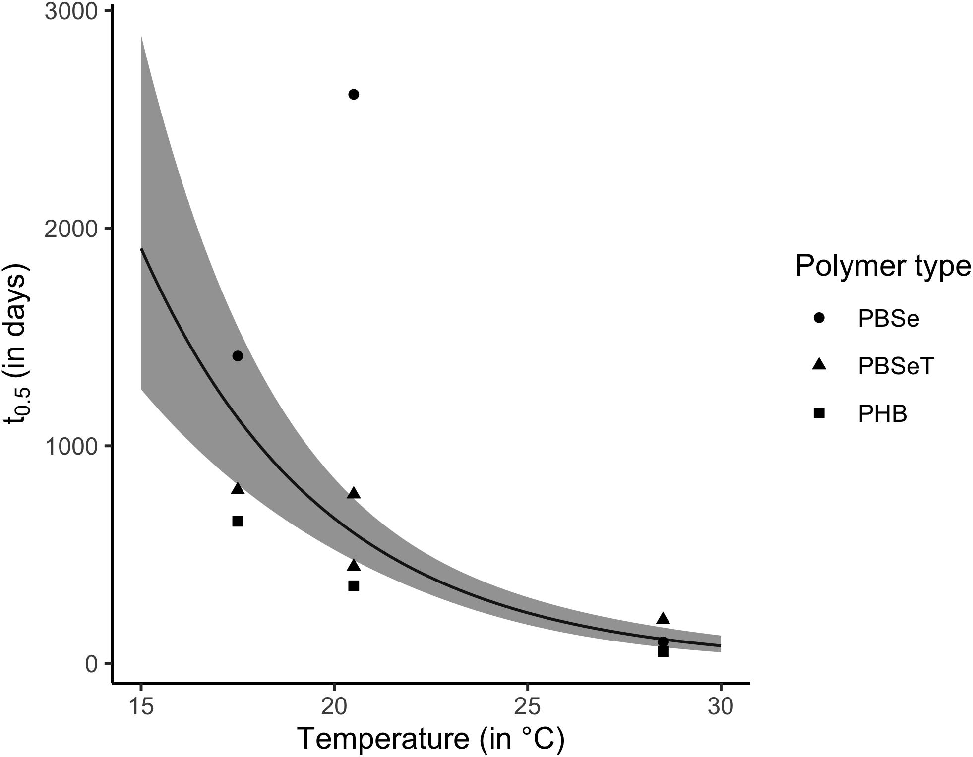
Figure 9. Temperature dependence of half-life in benthic tests: half-life t_0.5 decreases exponentially with temperature. The dots are the predicted half-life values for PHB (squares), PBSeT (triangles), and PBSe (circles). The line represents an exponential model, the shaded area is the standard error.

Other Factors That Determine Biodegradation

During the same EU project Open-Bio, Briassoulis et al. (2019) conducted similar field tests with the same test materials at a fish farm in Greece in a comparable temperature regime and reported complete disintegration of all samples in the benthic tests after 9 months, roughly accounting for a half-life of 140 days (estimated from the graphs provided) as compared to 738 days (PHB), 908 days (PBSe) and 1,070 days (PBSeT) in our Mediterranean benthic tests. This indicates that the trophic level of the habitat might also have a positive influence on the biodegradation activity (and rate). In our study, most of the nutrient-related parameters (sensu Weber et al., 2012) such as concentrations of N and P compounds were low in the three different settings. Manipulative tank experiments could be used to investigate the relationship between nutrient concentration and biodegradation rate.

The abundance of microbes and their community composition, especially in tests involving sediments, might differ strongly, e.g., dependent on factors such as grain size (Ahmerkamp et al., 2020). Different sediment types such as e.g., coarse permeable sand, fine silt, or mud due to their different permeabilities might favor strongly differing metabolic pathways, e.g., depending on the presence or absence of oxygen as an electron acceptor. Some polymers might also behave differently under oxic or anoxic conditions than others. As reported recently (Lott et al., 2020), we also observed a different disintegration performance within the same sample exposed in the HYDRA^® frames (SI Figure 1). Due to the tightly adhering frame, the margin of the exposed plastic film (which was not accounted for in the disintegration measurements) supposedly had less exchange with the surrounding water, and the microbes there presumably experienced hypoxic or anoxic conditions.

PHB and PBSe showed a contrasting trend in the performance in the benthic and eulittoral tests in the mesocosms experiment: PHB was disintegrating faster in the benthic than in the eulittoral and PBSe faster in the eulittoral than in the benthic. In the field tests, PHB and PBSeT disintegrated faster in the eulittoral than in the benthic, also the half-life predictions for PBSe followed this trend, but differences were not significant. In line with the results of the mesocosm tests discussed above, this is an indication that the comparison of a test material with a reference material has to be done with some caution and the application of a material as a positive control is critically scrutinized. Some well-degradable materials might perform differently under certain conditions than expected, making the desired intercalibration of test results e.g., between habitats or climate zones based on one material difficult and conclusions should be drawn with caution.

Creating Comparable Data for LC(I)A

The predictive modeling of half-lives we present here gives the opportunity to assign a numerical value for the biodegradation performance in a defined scenario (e.g., Mediterranean Sea/Pianosa Island/benthic sand) as a material property. Data provided in this manner by us and studies to come should be used for the compilation of a catalog of biodegradable materials and their properties with regard to their environmental performance that can be used for statistical comparisons of different materials in the same habitat, or one material in different environmental scenarios. These specific half-lives will also be suited to enable further mathematical modeling e.g., for environmental benefit and risk assessment and the life cycle (impact) assessment of products. Furthermore, such a catalog could help industry, public administration, and NGOs to base their decisions for or against certain materials and their application on facts.

The principle of half-life, however, is difficult to communicate and to perceive to non-specialists e.g., the general public or policy makers. The question “How long does it take?” (until a certain object is completely degraded) cannot be readily answered by the specific half-life.

Dilkes-Hoffman et al. (2019) compared the results of PHB biodegradation tests under marine conditions in a meta-analysis from eight former studies. To achieve comparability, they recalculated the data to a rate of mass loss over time per exposed surface area (Equation 3) based on the assumption that in biodegradable solids the processes causing the degradation are only happening at the surface of the object:

$r=\mathrm{\Delta }m\cdot A_{active}^{-1}\cdot t^{-1}(3)$

where m is mass, A the surface area exposed, and t the time.

From these data, they also estimated the lifetime, i.e., the time needed for an object to completely degrade. The 95% CI of the biodegradation rates derived from all studies considered was 0.04–0.09 mg cm^–2 d^–1. We applied their calculation method to our experimental results on PHB, using the volume of the films (area × thickness) and the specific gravity ρ of the material (ρ_PHB = 1.3). We obtained rates within or close to this range only for our fastest scenarios, PHB exposed in the benthic test in SE Asia (0.051 mg cm^–2 d^–1), and in lab tests (0.012 mg cm^–2 d^–1 for eulittoral and 0.024 mg cm^–2 d^–1 for benthic tests). For the other test scenarios, the biodegradation rates were one order of magnitude lower (Supplementary Table 9).

If we apply the minimum and maximum biodegradation rates derived from the results of our beach and seafloor field tests in the Mediterranean Sea and in tropical SE Asia (0.051–0.004 mg cm^–2 d^–1; Supplementary Table 9) to estimate the lifetime of the PHB objects as in Figure 3 of Dilkes-Hoffman et al. (2019) it results in lifetimes 1.8–10 times higher, ranging from 2–20 months for a 35 μm thick shopping bag to 2.7–36 years for a PHB bottle with 800 μm thickness to 4–54 years for PHB cutlery (∼1,300 μm). It has, however, to be taken into account, that the calculation of the rate by Dilkes-Hoffman et al. (2019) is based on the initial surface of the object which in reality will change during the biodegradation process. Very likely, the surface roughness will increase and the surface-to-volume ratio will become higher and thus the gross degradation of the object or its fragments will accelerate, as was also shown by Chinaglia et al. (2018). Therefore, these estimations should be taken as conservative for the environments considered. On the other hand, given the strong temperature dependence of the biodegradation rate, it can be assumed that in colder environments as the deep sea or in polar regions the lifetime will be higher.

The dependence of the (bulk) biodegradation rate on the surface-to-volume (or mass) ratio was mentioned by Modelli et al. (1999) who, in a study with another focus, compared powder (grain size 1 μm) and film of PHB (4 cm × 4 cm × 0.025 cm) in a soil biodegradation test according to ASTM (2003) and interpreted the rates as different. The authors missed to numerically address the surface-to-volume ratio in this comparison and stated that the initial rate (11 % of the 0.5 g bulk polymer in 1 day) was 90 times higher for powder deduced from the slope of the linear fits. However, if their data is re-calculated with Equation 3, the rates of 0.023 [0.056 g ⋅ d^–1; A = 2,400 cm²] for powder (simplified assuming spherical particles) and 0.020 [0.132 g ⋅ 210 d^–1; A = 32 cm²] for film are almost identical and the difference in the bulk rates (90 times) is well explained by the difference in surface area (75 times).

Chinaglia et al. (2018) tested also in soil (ASTM, 2003) lab experiments at 28 ± 2°C, PBSe powder of different grain sizes and found the maximum rate for 1 g of sample at 97 mg C_polymer d^–1 (and the total surface in dependence of grain size where half the maximum rate was reached at 1,122 cm²). If equation 3 is applied to their data, the areal rates for PBSe particles (0.05–0.18 mg. cm². d^–1) are about 10 to 600 times higher than our results for PBSe film (25 μm thickness) under marine conditions (Supplementary Table 10).

Taking into account that biodegradation of a solid object is occurring at the surface the specific half-lives modeled from results from our tests with film can be converted to erosion rates in μm per year yr by dividing half the film thickness h by the half-life t_0.5:

$r[\mathrm{\mu }m\cdot y{r}^{-1}]=(\frac{0.5h}{t_{0.5}})\cdot 365(4)$

These values are surface-independent and density-independent and can be applied to three-dimensional objects with parallel surfaces as e.g., most packaging such as bottles etc., with the only object-specific parameter to know being the material thickness.

Applying Equation 4, microbial surface erosion (“micro-bioerosion”) rates derived from our experimental results range from 12.4–285.7 μm ⋅ year^–1 for PHB, 5.7–31.1 μm ⋅ year^–1 for PBSeT and 1.7–46.0 μm ⋅ year^–1 for PBSeT (see Table 4).

TABLE 4

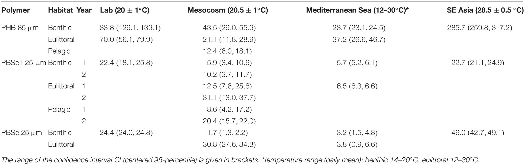
Table 4. Surface micro-bioerosion rates (μm ⋅ yr^–1) of PHB, PBSe, and PBSeT under different marine conditions.

The micro-bioerosion rate in the respective habitat divided by the wall thickness in μm of an object will provide estimated lifetimes that can be used for environmental risk and life cycle assessments. Further experiments on solid objects rather than the film will be useful to validate these estimations.

The numbers presented here might also help to clarify the assumption that degradation of biodegradable plastic in the marine environment is occurring “much more slowly” and give useful input to the statement that “the degree to which “biodegradable” plastics actually biodegrade in the natural environment is subject to intense debate” (UNEP, 2015). Our data and also previous studies show that there are biodegradable plastic materials that do degrade relatively fast in the natural marine environment given their functional properties in the applications they were designed for. A stable, durable, and resistant plastic item that performs well during use is unlikely to “disappear” within a few days or weeks once lost or littered to the natural environment. This also underpins the urgency to apply all possible means to prevent any plastic material from entering the natural environment, being it biodegradable or not. Plastic lost to the environment is pollution, even if biodegradable. However, biodegradable plastics are less likely to accumulate or persist than conventional plastics.

Conclusion

The large spectrum of scenarios in which biodegradation tests were conducted here revealed a high variability in the rate of biodegradation of biodegradable plastics under marine conditions and confirms the impreciseness of the term “marine biodegradable.” The specific half-lives differed by orders of magnitude from weeks to years and give a deep insight into the possible range of the real performance of biodegradable plastics in the open environment. The data also demystifies the assumption that in the marine environment in general the biodegradation of biodegradable plastics is slow. Although several scenarios such as the very cold habitats (deep sea, high latitudes) and areas with little or no oxygen (mainly with fine sediments) have not been touched by our study biodegradation was observed to occur to a certain extent under all conditions considered. This differentiated view together with numerically comparable rates will be useful for the estimation of the environmental persistence of biodegradable plastics in the sea in comparison to conventional plastic materials. This study also will deliver urgently sought-after base data for the assessment of benefits and risks of biodegradable plastics with regards to their environmental performance.

Data Availability Statement

The original contributions presented in the study are included in the article/Supplementary Material, further inquiries can be directed to the corresponding author/s.

Ethics Statement

Written informed consent was obtained from the individual for the publication of any potentially identifiable images or data included in this article.

Author Contributions

CL, MW, DM, BU, MvE, ES, AE, and MR designed experiments, conducted lab (MvE, ES), mesocosm and field experiments. AE, CL, MW, MvE, and ES analyzed data. AE performed statistical modeling. ML supervised field studies in Indonesia. CL, MW, and AE wrote the manuscript with input of all coauthors. All authors contributed to the article and approved the submitted version.

Funding

The study was in part conducted within the European Union’s FP7 project Open-Bio and has received partial funding under the grant agreement no KBBE/FP7EN/613677. The authors declare that this study received additional funding from BASF SE, Ludwigshafen, Germany. The funder was not involved in the study design, collection, analysis, interpretation of data, the writing of this article or the decision to submit it for publication. Novamont S.p.A., Novara, Italy provided film for tests during the Open-Bio project.

Conflict of Interest

CL, AE, and MW were employed by HYDRA Marine Sciences GmbH. DM and BU were employed by HYDRA Fieldwork GbR. MvE and ES were employed by LeAF BV.

The remaining authors declare that the research was conducted in the absence of any commercial or financial relationships that could be construed as a potential conflict of interest.

Acknowledgments

Deep thanks to the student assistants and interns of HYDRA for their help during experiment preparation and sampling. Special thanks for technical work to Eskil Salis Gross for sediment characterization, to Nora Pauli, Alexandra Belitz and Esther Thomsen for image analysis. We also thank the National Park Tuscan Archipelago, Portoferraio for granting access to the protected area of the Island of Pianosa with the research permit n.3063/19.05.2014 and following. Dott. Emiliano Somigli and his staff are gratefully acknowledged for their support and for granting access to Terme San Giovanni to perform the eulittoral tests. We also thank Giorgio Vendetti from Hotel Mirage, Marina di Campo, for providing meteorological data (www.elbaexplorer.com). The Government of the Republic of Indonesia, Ministry of Research, Technology and Higher Education, RISTEK-DIKTI, Jakarta is gratefully thanked for granting the research permits no. 71 and 72/SIP/FRP/E5/Dit.KI/III/2017 and extensions to CL and MW, CL, and MW express their thanks to University Sam Ratulangi, Manado welcoming them as guest researchers. Thanks to Ilaria Reggi, Anna Clerici, Marco Perin, and staff of Coral Eye Resort and Coral Research Outpost, Bangka Island, Sulawesi Utara, Indonesia for technical support and maintenance. The study in the Mediterranean Sea was conducted within the European Union’s FP7 project Open-Bio and has received partial funding under the grant agreement no KBBE/FP7EN/613677 and by BASF SA, Ludwigshafen, Germany. Thanks also to Novamont S.p.A., Novara, Italy for providing film for tests during the Open-Bio project. We also thank our partners of the WP5 of the Open-Bio project for valuable discussions on the outcomes of the tests.

Supplementary Material

The Supplementary Material for this article can be found online at: https://www.frontiersin.org/articles/10.3389/fmars.2021.662074/full#supplementary-material

Footnotes

1. ^ https://imagej.nih.gov/ij/

References

Ahmerkamp, S., Marchant, H., Peng, C., Probandt, D., Littmann, S., Kuypers, M. M. M., et al. (2020). The effect of sediment grain properties and porewater flow on microbial abundance and respiration in permeable sediments. Sci. Rep. 10:3573. doi: 10.1038/s41598-020-60557-7

PubMed Abstract | CrossRef Full Text | Google Scholar

Albertsson, A. C., Bødtker, G., Boldizar, A., Filatova, T., Prieto Jimenez, M. A., Loos, K., et al. (2020). Biodegradability of Plastics in the Open Environment. Science Advice for Policy by European Academies, Evidence Review Report no. 8. Berlin: Science Advice for Policy by European Academies, 231. doi: 10.26356/biodegradabilityplastics

CrossRef Full Text | Google Scholar

Ambrosini, R., Azzoni, R. S., Pittino, F., Diolaiuti, G., Franzetti, A., and Parolini, M. (2019). First evidence of microplastic contamination in the supraglacial debris of an alpine glacier. Environ. Pollut. 253, 297–301. doi: 10.1016/j.envpol.2019.07.005

PubMed Abstract | CrossRef Full Text | Google Scholar

ASTM (2003). ASTM D5988-03: Standard Test Method for Determining Aerobic Biodegradation in Soil of Plastic Materials or Residual Plastic Materials After Composting. West Conshohocken, PA: ASTM International, doi: 10.1520/D5988-03

PubMed Abstract | CrossRef Full Text | Google Scholar

ASTM (2017). ASTM D6691-17: Standard Test Method for Determining Aerobic Biodegradation of Plastic Materials in the Marine Environment by a Defined Microbial Consortium or Natural Sea Water Inoculum. West Conshohocken, PA: ASTM International, doi: 10.1520/D6691-17

PubMed Abstract | CrossRef Full Text | Google Scholar

Bagheri, A. R., Laforsch, C., Greiner, A., and Agarwal, S. (2017). Fate of so-called biodegradable polymers in seawater and freshwater. Glob. Chall. 1:1700048. doi: 10.1002/gch2.201700048

PubMed Abstract | CrossRef Full Text | Google Scholar

Böer, S. I., Arnosti, C., van Beusekom, J. E. E., and Boetius, A. (2009). Temporal variations in microbial activities and carbon turnover in subtidal sandy sediments. Biogeosciences 6, 1149–1165. doi: 10.5194/bg-6-1149-2009

CrossRef Full Text | Google Scholar

Briassoulis, D., Pikasi, A., Briassoulis, C., and Mistriotis, A. (2019). Disintegration behaviour of bio-based plastics in coastal zone marine environments: a field experiment under natural conditions. Sci. Total Environ. 688, 208–223. doi: 10.1016/j.scitotenv.2019.06.129

PubMed Abstract | CrossRef Full Text | Google Scholar

Briassoulis, D., Pikasi, A., Papardaki, N. G., and Mistriotis, A. (2020). Aerobic biodegradation of bio-based plastics in the seawater/sediment interface (sublittoral) marine environment of the coastal zone – Test method under controlled laboratory conditions. Sci. Total Environ. 722:137748. doi: 10.1016/j.scitotenv.2020.137748

PubMed Abstract | CrossRef Full Text | Google Scholar

Chinaglia, S., Tosin, M., and Degli Innocenti, F. (2018). Biodegradation rate of biodegradable plastics at molecular level. Polym. Degrad. Stab. 147, 237–244. doi: 10.1016/j.polymdegradstab.2017.12.011

CrossRef Full Text | Google Scholar

Dilkes-Hoffman, L. S., Lant, P. A., Laycock, B., and Pratt, S. (2019). The rate of biodegradation of PHA bioplastics in the marine environment: a meta-study. Mar. Pollut. Bull. 142, 15–24. doi: 10.1016/j.marpolbul.2019.03.020

PubMed Abstract | CrossRef Full Text | Google Scholar

Dris, R., Gasperi, J., Saad, M., Mirande, C., and Tassin, B. (2016). Synthetic fibers in atmospheric fallout: a source of microplastics in the environment? Mar. Pollut. Bull. 104, 290–293. doi: 10.1016/j.marpolbul.2016.01.006

PubMed Abstract | CrossRef Full Text | Google Scholar

European Bioplastics (2020). Bioplastics Market Development Update 2020. Berlin: European Bioplastics, 2. Available online at: https://docs.european-bioplastics.org/conference/Report_Bioplastics_Market_Data_2020_short_version.pdf (accessed January 05, 2021).

Google Scholar

European Commission (2018). A European Strategy for Plastics in a Circular Economy. Brussels: European Commission, 24. Available online at: https://ec.europa.eu/environment/circular-economy/pdf/plastics-strategy-brochure.pdf

Google Scholar

European Commission (2019). The European Green Deal. Brussels: European Commission. Available online at: https://eur-lex.europa.eu/resource.html?uri=cellar:b828d165-1c22-11ea-8c1f-01aa75ed71a1.0002.02/DOC_1&format=PDF (accessed December 11, 2019).

Google Scholar

Gazzetta Ufficiale della Repubblica Italiana (2017). Decreto Legge del 20 Giugno 2017, n. 91, Conv. Con Mod. Nella L. 3 Agosto 2017, n. 123, Art. 9 and 9bis. Rome: Gazzetta Ufficiale della Repubblica Italiana. Available online at: https://www.gazzettaufficiale.it/eli/id/2017/08/12/17A05735/sg (accessed January 5, 2021).

Google Scholar

Geyer, R., Jambeck, J. R., and Law, K. L. (2017). Production, use, and fate of all plastics ever made. Sci. Adv. 3:e1700782.

Google Scholar

Harrison, J. P., Boardman, C., O’Callaghan, K., Delort, A.-M., and Song, J. (2018). Biodegradability standards for carrier bags and plastic films in aquatic environments: a critical review. R. Soc. Open Sci. 5:171792. doi: 10.1098/rsos.171792

PubMed Abstract | CrossRef Full Text | Google Scholar

Helmberger, M. S., Tiemann, L. K., and Grieshop, M. J. (2019). Towards an ecology of soil microplastics. Funct. Ecol. 34, 550–560. doi: 10.1111/1365-2435.13495

CrossRef Full Text | Google Scholar

Holm, S. (1979). A simple sequentially rejective multiple test procedure. Scand. J. Stat. 6, 65–70.

Google Scholar

International Organization for Standardization (2016). ISO 19679:2016 “Plastics – Determination of Aerobic Biodegradation of Non-Floating Plastic Materials in a Seawater/Sediment Interface – Method by Analysis of Evolved Carbon Dioxide”. Geneva: International Organization for Standardization.

Google Scholar

International Organization for Standardization (2019). ISO 22404:2019 “Plastics – Determination of the Aerobic Biodegradation of Non-Floating Materials Exposed to Marine Sediment – Method by Analysis of Evolved Carbon Dioxide”. Geneva: International Organization for Standardization.

Google Scholar

Journal Officiel de la République Française (2016). Décret no 2016-379 du 30 mars 2016 Relatif aux Modalités de Mise en æuvre de la Limitation des sacs en Matières Plastiques à Usage unique. Journal officiel électronique authentifié n° 0076 du 31/03/2016. Paris: Journal Officiel de la République Française. Available online at: https://www.legifrance.gouv.fr/download/pdf?id=7Ix6f05i9MKyCu64o4E403m5ifQeOmNVXdsTzHrVmHE= (accessed January 5, 2021).

Google Scholar

Junker, T., Coors, A., and Schüürmann, G. (2016). Development and application of screening tools for biodegradation in water – sediment systems and soil. Sci. Total Environ. 544, 1020–1030.

Google Scholar

Kanhai, L. D. K., Gardfeldt, K., Krumpen, T., Thompson, E. C., and O’Connor, I. (2020). Microplastics in sea ice and seawater beneath ice floes from the Arctic Ocean. Sci. Rep. 10:5004. doi: 10.1038/s41598-020-61948-6

PubMed Abstract | CrossRef Full Text | Google Scholar

Lott, C., Eich, A., Unger, B., Makarow, D., Battagliarin, G., Schlegel, K., et al. (2020). Field and mesocosm methods to test biodegradable plastic film under marine conditions. PLoS One 15:e0236579. doi: 10.1371/journal.pone.0236579

PubMed Abstract | CrossRef Full Text | Google Scholar

Lott, C., Weber, M., Makarow, D., Unger, B., Pikasi, A., Briassoulis, D., et al. (2016a). Marine Degradation Test Field Assessment. European Commission, Project “Open-BIO”, KBBE/FP7EN/613677, WP5-D5.8. Available online at: https://www.biobasedeconomy.eu/app/uploads/sites/2/2017/09/Open-Bio_D5.8_summary.pdf (accessed January 5, 2021).

Google Scholar

Lott, C., Weber, M., Makarow, D., Unger, B., Pognani, M., Tosin, M., et al. (2016b). Marine Degradation Test Assessment: Marine Degradation Test of Bio-Based Materials at Mesocosm Scale Assessed. European Commission, Project “Open-BIO”, KBBE/FP7EN/613677, WP5-D5.7 Part 2. Available online at: https://www.biobasedeconomy.eu/app/uploads/sites/2/2017/07/Open-BioD5.7_public-summary.pdf (accessed January 5, 2021).

Google Scholar

Mistriotis, A., Papardaki, N. G., and Provata, A. (2019). Biodegradation of cellulose in laboratory-scale bioreactors: experimental and numerical studies. J. Polym. Environ. 27, 2793–2803. doi: 10.1007/s10924-019-01560-6

CrossRef Full Text | Google Scholar

Modelli, A., Calcagno, B., and Scandola, M. (1999). Kinetics of aerobic polymer degradation in soil by means of the ASTM D 5988-96 standard method. J. Environ. Polym. Degrad. 7, 109–116.

Google Scholar

Payne, W. J. (1970). Energy yields and growth of heterotrophs. Annu. Rev. Microbiol. 24, 17–52.

Google Scholar

Pischedda, A., Tosin, M., and Degli Innocenti, F. (2019). Biodegradation of plastics in soil: The effect of temperature. Polym. Degrad. Stab. 170:109017. doi: 10.1016/j.polymdegradstab.2019.109017

CrossRef Full Text | Google Scholar

R Core Team (2020). R: A Language and Environment for Statistical Computing. Vienna: R Foundation for Statistical Computing.

Google Scholar

Republic of Indonesia (2017). Indonesia’s Plan of Action on Marine Plastic Debris 2017–2025, 2017. [Internet] Executive Summary. Available online at: https://marinelitternetwork.engr.uga.edu/wp-content/uploads/2017/07/Marine-Plastic-Debris-Indonesia-Action.pdf (accessed Jan 10, 2019).

Google Scholar

Rouch, D. (2019). Plastic Future: How to Reduce the Increasing Environmental Footprint of Plastic Packaging. Report, 42 p. [Internet]. Available online at: https://www.researchgate.net/publication/337506127 (accessed January 5, 2021).

Google Scholar

Schmidt, J. L., Deming, J. W., Jumars, P. A., and Keil, R. G. (1998). Constancy of bacterial abundance in surficial marine sediments. Limnol. Oceanogr 43, 976–982.

Google Scholar

Sintim, H. Y., and Flury, M. (2017). Is biodegradable plastic mulch the solution to agriculture’s plastic problem? Environ. Sci. Technol. 2017, 1068–1069. doi: 10.1021/acs.est.6b06042

PubMed Abstract | CrossRef Full Text | Google Scholar

Smithson, M., and Verkuilen, J. (2006). A better lemon squeezer? maximum-likelihood regression with beta-distributed dependent variables. Psychol. Methods 11, 54–71.

Google Scholar

Tosin, M., Weber, M., Siotto, M., Lott, C., and Degli Innocenti, F. (2012). Laboratory test methods to determine the degradation of plastics in marine environmental conditions. Front. Microbiol 3:225. doi: 10.3389/fmicb.2012.00225

PubMed Abstract | CrossRef Full Text | Google Scholar

UNEP (2015). Biodegradable Plastics and Marine Litter. Misconceptions, concerns and Impacts on Marine Environments. Nairobi: United Nations Environment Programme (UNEP).

Google Scholar

Wagner, M., Scherer, C., Alvarez-Muñoz, D., Brennholt, N., Bourrain, X., Buchinger, S., et al. (2014). Microplastics in freshwater ecosystems: what we know and what we need to know. Environ. Sci. Eur. 26:12. doi: 10.1186/s12302-014-0012-7

PubMed Abstract | CrossRef Full Text | Google Scholar

Weber, M., de Beer, D., Lott, C., Polerecky, L., Kohls, K., Abed, R. M. M., et al. (2012). Mechanisms of damage to corals exposed to sedimentation. Proc. Natl. Acad. Sci. U.S.A. 24, E1558–E1567. doi: 10.1073/pnas.1100715109

PubMed Abstract | CrossRef Full Text | Google Scholar

Weber, M., Lott, C., van Eekert, M., Mortier, M., Siotto, M., de Wilde, B., et al. (2015). Review of Current Methods and Standards Relevant to Marine Degradation. European Commission, Project “Open-BIO”, KBBE/FP7EN/613677, WP5-D5.5, 90 pp. Available online at: http://www.biobasedeconomy.eu/media/downloads/2015/10/Open-Bio-Deliverable-5.5-Review-of-current-methods-and-standards-relevant-to-marine-degradation-Small.pdf (accessed January 5, 2021).

Google Scholar