 Melissa Cook
 Jaymie L. Reneker
 Redwood W. Nero3
 Brian A. Stacy
 David S. Hanisko
 Zhankun Wang
94% of researchers rate our articles as excellent or good
Learn more about the work of our research integrity team to safeguard the quality of each article we publish.
Find out more
ORIGINAL RESEARCH article
Front. Mar. Sci., 16 June 2021
Sec. Marine Megafauna
Volume 8 - 2021 | https://doi.org/10.3389/fmars.2021.659536
This article is part of the Research TopicAdvances in Understanding Sea Turtle Use of the Gulf of MexicoView all 17 articles
Stranded sea turtles provide valuable information about causes of mortality that threatens these imperiled species. Many potential factors determine whether drifting sea turtles are deposited on shore, discovered by people, and reported to stranding networks resulting in successful documentation. We deployed 182 sea turtle cadavers and 115 wooden effigy drifters with affixed GPS-satellite tags to study stranding probability in the northern Gulf of Mexico (nGOM) in an effort to better understand seasonal stranding variations in this region. Public reports of beached carcasses were recorded to determine reporting rates. Season and distance from shore greatly influenced beaching results. During winter months when strandings are infrequent and sea turtle abundance is likely low in cold nearshore waters, carcasses had an 80–90% probability of beaching. Beaching probability was reduced to 37–50% during the spring, which is the period of greatest strandings in this region. During summer months when relatively few strandings are documented, the probability of a carcass beaching dropped to only 4–8%. Low summer stranding rates were coincident with higher rates of decomposition (7%) attributed to warmer water temperatures, more frequent scavenging (69% of carcasses), and shifting wind and current patterns which drive carcasses offshore or to remote locations. As waters cooled in the fall, probability of carcasses beaching increased to 40–48%, coincident with a small pulse in strandings that often occurs during this period. Only 28% of carcasses and effigies came ashore on mainland beaches and were easily available for discovery by the public, 49% were on barrier islands that are publicly accessible and 23% beached in dense salt marshes where discovery would be unlikely. The 47% of objects that did not beach included those lost at sea and carcasses that were likely scavenged or decomposed. Only 22% of beached carcasses were reported due to infrequent (11%) reporting on barrier islands. Notably, only 50% of carcasses deposited on mainland beaches were reported, which was lower than anticipated. We recommend additional efforts to increase reporting rates of carcasses by the public and use of dedicated surveys to detect stranded sea turtles, especially on barrier islands in this region.
Sea turtle strandings are one of the few direct indicators of at-sea mortality. Stranding data provide critical information about mortality sources, locations where such threats occur, and other informative characteristics, such as temporospatial trends (e.g., Mancini et al., 2011; Koch et al., 2013; Foley et al., 2019). However, the number of documented sea turtle strandings only represents a minimum measure of mortality, as the probability that a dead or impaired sea turtle will drift ashore and become documented is influenced by oceanographic and atmospheric conditions, decomposition and scavenging rates, shoreline characteristics, as well as the extent of human presence and the effectiveness of detection, and reporting mechanisms. These factors, particularly those related to environmental conditions, can be highly variable by locality and time of year.
Previous studies conducted in the United States south Atlantic derived mortality estimates using stranding data (Epperly et al., 1996; Hart et al., 2006). By comparing observer data and stranding reports, Epperly et al. (1996) determined the number of strandings on North Carolina beaches represented only 7–13% of the estimated fishery-induced mortality. They also noted that strandings during the winter months were a poor indicator of at-sea mortalities because carcasses were often transported offshore by bottom currents. Hart et al. (2006) evaluated the influence of nearshore physical oceanographic and wind regimes on sea turtle strandings to decipher seasonal trends and stranding patterns on North Carolina oceanfront beaches. To accomplish this, results from 1967 and 1973 oceanographic drift bottle experiments were reevaluated and used in conjunction with stranding data. Return rates of drift bottle experiments provided an upper limit estimate that only 20% of sea turtle carcasses will strand on local beaches. Findings suggest that carcasses are only likely to strand if mortality occurs within 20 km or less from shore. Mortalities occurring farther from shore have an even lower, perhaps negligible, probability of stranding on beaches. Additionally, the probability of a carcass stranding varies by season due to variable oceanographic conditions (Hart et al., 2006). Koch et al. (2013) also used drifters combined with stranding data and found similar results off Baja California Sur; stranding rates varied widely and usually do not exceed 10–20% of total mortality, even in nearshore waters.
Despite the importance of stranding (and reporting) probability in the use of stranding-derived data, there have been very few studies of this topic and none in the Gulf of Mexico (GOM). Because strandings are influenced by oceanographic and seasonal conditions, the probability of carcasses stranding in the GOM could be considerably different than reported elsewhere. The United States South Atlantic Bight (SAB), which is the closest area previously studied, is generally a more energetic region in comparison to the northern Gulf of Mexico (nGOM). The SAB is strongly influenced by the Gulf Stream on its outer shelf and has greater overall wind generated wave and current fields than occur in the nGOM. Seasonal shifts in atmospheric conditions favoring onshore drift in spring and early summer, transitioning to conditions favoring offshore flows in fall and winter, occur in both systems. However, the more northerly latitude of the SAB results in a stronger pre-frontal setup, frontal passage, and return current flow than the nGOM. The nGOM attains higher spring and summer inshore temperatures, resulting in more benign winds, current flows, and likely faster decomposition of carcasses.
Beginning in 2010, the Sea Turtle Stranding and Salvage Network (STSSN) documented high numbers of strandings, primarily of Kemp’s ridley (Lepidochelys kempii) sea turtles, along the Mississippi (MS), Alabama (AL), and Louisiana (LA) coasts (STSSN1). Surveillance and documentation of sea turtle strandings in this region was highly variable prior to this period and was enhanced considerably following the Deepwater Horizon oil spill in April 2010. Over the last decade, sea turtle strandings have exhibited a relatively consistent seasonal occurrence characterized by peak activity during March to June followed by a marked reduction during summer months and slight resurgence in the fall (October–November). Necropsy findings also have been consistent and indicate a sudden cause of mortality in the majority of these strandings based on normal body mass, evidence of recent feeding prior to death (often on fin fish), frequent presence of sediment within the respiratory tract, and absence of significant disease or other apparent cause (Stacy, 2014). These findings are similar to previous reports of mortality attributed to incidental capture (bycatch) by fisheries (Shoop and Ruckdeschel, 1982; Shaver, 1991; Caillouet et al., 1996; Casale et al., 2010); however, a specific cause(s) of the spring peaks in strandings on the nGOM coast remains unidentified. Better understanding of the drivers of seasonal variation and distribution of strandings could significantly improve ongoing mortality monitoring and investigation, and enable comparisons of stranding data with anthropogenic activities of concern.
The objectives of this study were to (1) use floating sea turtle cadavers and effigy drifters to determine how environmental conditions influence seasonal variability in sea turtle stranding patterns in MS, where many nGOM strandings are found and (2) determine the proportion of stranded sea turtles originating from nGOM waters reported to the STSSN. By using actual sea turtle carcasses, we were able to determine the percent of dead turtles that strand on nGOM beaches as well as the effectiveness of stranding detection and reporting. Our methodology has wide applications for use to determine stranding probabilities and detection in other regions. Improved information on stranding rates will help scientists and managers further understand how reported strandings relate to total mortality and potential causes in the nGOM.
All carcasses used in this study were sea turtles that died during cold-stunning events, which occur when nearshore water temperatures persistently fall below 10°C in susceptible localities in the Atlantic and GOM. These events provide the most readily available source of non-decomposed carcasses for research purposes. All sea turtles were determined dead by qualified, permitted individuals based on absence of detectable cardiac contraction and were frozen at 0°C until use. We previously studied decomposition rates of unfrozen or frozen sea turtle carcasses and found no differences that are pertinent to our study objectives (Cook et al., 2020). Kemp’s ridley (Lepidochelys kempii, n = 57) and green (Chelonia mydas, n = 125) sea turtles were used based on availability. Carcasses ranged in size from 18.4 to 38.9 cm straight carapace length (SCL) (mean = 27.2 cm SCL).
Prior to deployment, frozen sea turtle carcasses were flipper tagged for identification, thawed in a water bath, and allowed to decompose until they achieved positive buoyancy due to accumulation of postmortem gases. This treatment ensured postmortem condition was similar among study animals and was developed to resemble the state at which dead turtles first reach the surface and begin to drift (Reneker et al., 2018). The target carcass condition was <50% of the carapace exposed above the waterline and all appendages underwater at the time of deployment. The use of actual bloated sea turtle carcasses allowed for us to incorporate natural decomposition and scavenging into our study design.
In addition to sea turtle carcasses, wooden effigies were deployed for comparison. The use of an effigy removed the influence of decomposition and scavenging and allowed us to monitor object drift and temporal trends in strandings with greater sample sizes. Effigy use also offered the potential for comparison to future studies where use of actual turtles is infeasible. Wood-block effigies were constructed of three square pieces of commercial southern yellow pine (middle block, 11.25″ × 11.25″ × 1.5″; upper and lower blocks, 5.5″ × 5.5″ × 1.5″) centered and attached with glue and screws. Small, 2″ × 3″ × 1″ SPOT Trace (SPOT) GPS satellite transmitters were vacuum sealed in plastic, placed in small 0.5 L plastic jars and attached to all carcasses and effigies using 4 mm braided polyethylene twine. The twine was tied through a hole drilled through the effigy or marginal bone of the carcasses. The jars were positioned so they would float approximately 30 cm behind the objects (Figure 1). The SPOT transmitted locations every 10 min and battery life lasted an average of 27 days before the signal was lost. GPS location was accurate to within a meter and objects were monitored in real-time over the course of their deployment.
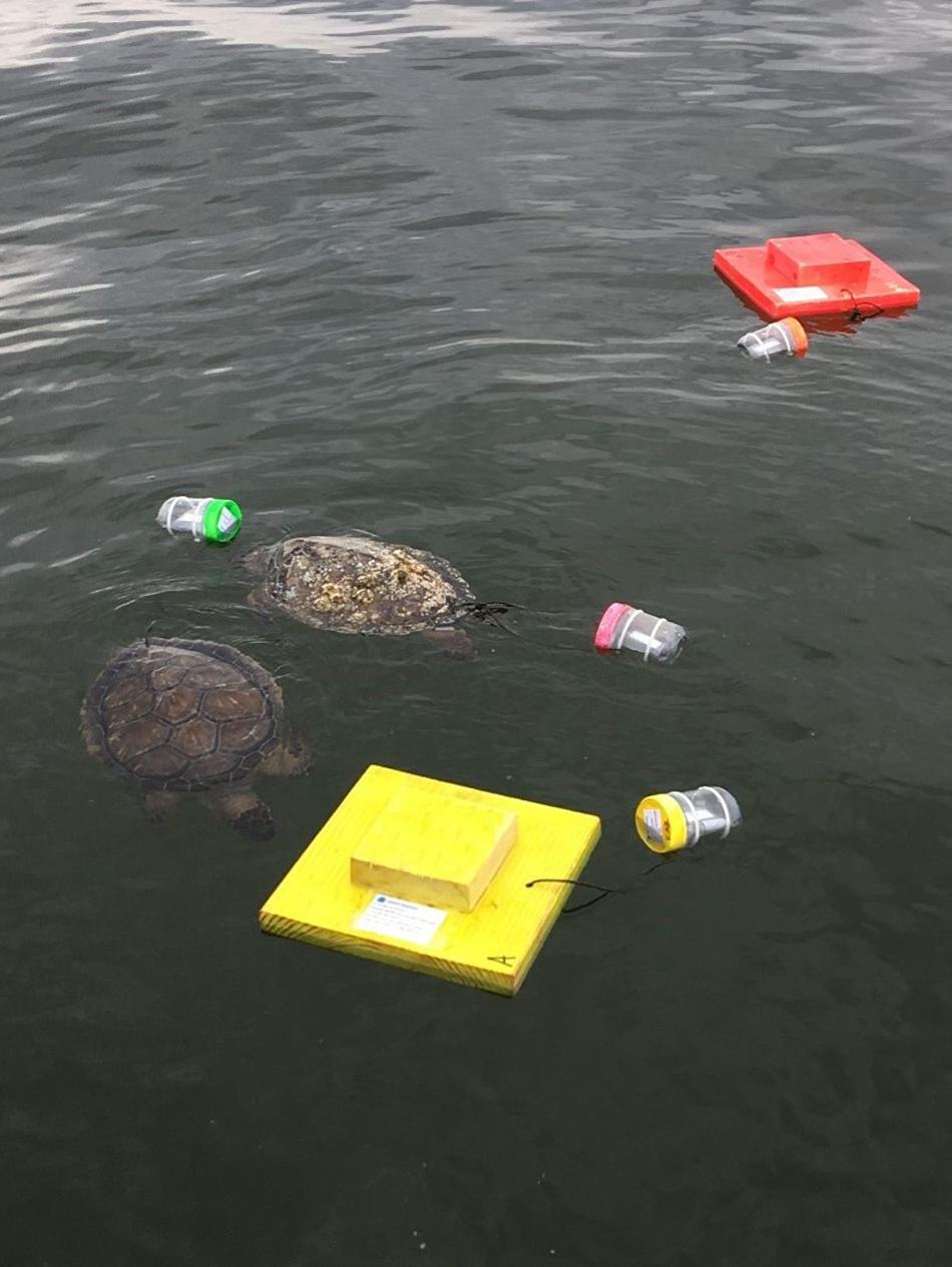
Figure 1. Sea turtle carcasses, wood effigies and satellite tags at deployment location.
Sea turtle carcass and effigy deployments began in January of 2017, in coastal and offshore waters in the nGOM. Deployments occurred at five sites (Figure 2) selected in areas with documented sea turtle occurrence (Coleman et al., 2016), known shrimping effort, or in areas of other potential mortality sources (i.e., ship traffic). Sites were also selected in various depths because the time required for a dead sea turtle to decompose and float, in the case of sinking carcasses, varies depending on temperature and depth (influenced by water pressure) (Cook et al., 2020). More gases are needed to float at greater depths. For example, if the bottom temperature was 24°C at the three sites, the time required for a carcass to float would increase from ∼1.5 days (at 5 m), ∼2.5 days (at 10 m), and ∼5.3 days (at 25 m) as depth increased. Drift studies consisted of both biweekly (sites A, B, and C) and monthly (sites D, E) deployments (Figure 2 and Table 1).
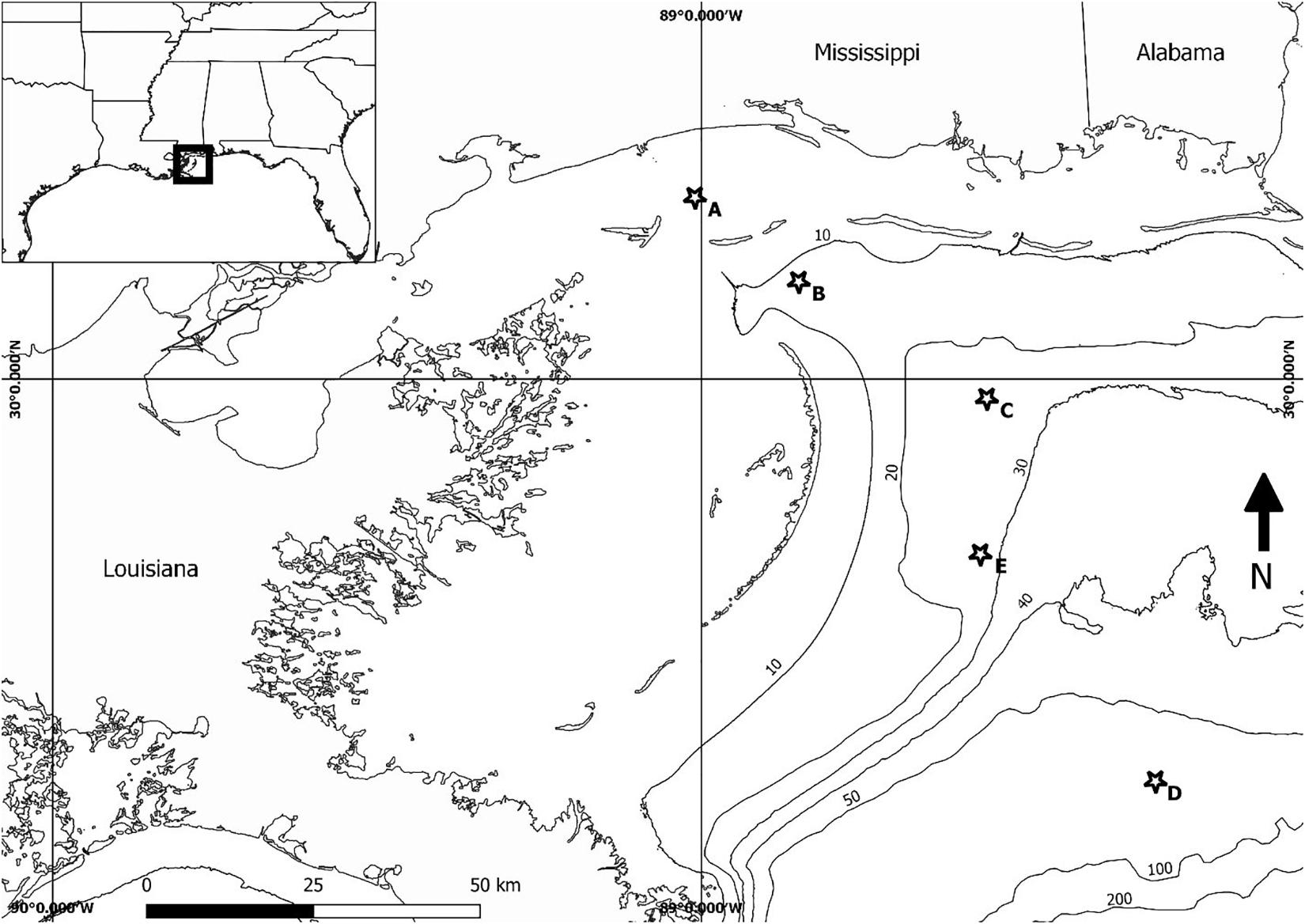
Figure 2. Sea turtle carcass and wood effigy deployment locations. Deployments occurred twice a month from January to December at sites A, B, C and monthly from February–May and July at sites D and E. Depth contours are in meters.
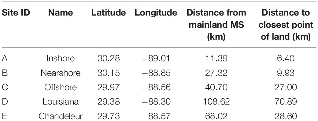
Table 1. Location of carcass and effigy deployments.
Approximately every 2 weeks, from January through December 2017, a deployment date was chosen based on favorable weather conditions. For each deployment, 2–3 bloated sea turtle carcasses (Reneker et al., 2018) and 1–3 wooden effigies, hereafter referred to collectively as floating “objects,” were released at three pre-selected deployment locations (A,B, and C), which were ∼11, 27, and 41 km, respectively, from mainland MS. In addition, five monthly deployments were conducted in February–May and July at sites ≥68 km from mainland MS (D,E). The objective of these two more distant sites was to determine the maximum distance a carcass could drift and still strand in MS. Due to logistics, only wooden effigies were used for the monthly, distant deployments. The first two deployments occurred at Site D (110 km from mainland MS). Drift tracks from the first two deployments indicated objects that far south of MS would likely never beach on the MS mainland or barrier islands. Therefore, the site location was moved to Site E (68 km from mainland MS) for the remaining three deployments.
At each deployment site, sea turtle carcasses and effigies were released off the side of the boat simultaneously. GPS location, deployment time, weather, and sea conditions were recorded. A YSI-85 was used to measure dissolved oxygen, temperature, and salinity of the surface water at each deployment location. Air temperature, wind speed, and wind direction were collected with an anemometer. Photographs and video were taken for reference. Once objects were deployed, they were allowed to float naturally with the winds and currents. We observed them for ∼10 min to ensure nothing was tangled and all were floating well before departing. Real-time monitoring occurred throughout the entire deployment to determine where objects travelled, if a transmitter stopped working, or if the object came ashore. At the conclusion of each deployment, carcasses and effigies were assigned outcomes of beached or did not beach. Objects were classified as beached if the object came ashore with the SPOT still attached. Outcomes classified as not beached included instances where the tag ceased transmitting or when the carcass/effigy was never recovered. Secondary determinations were made when only SPOT tags beached. If we recovered a SPOT without the turtle attached, we attributed the loss to probable scavenging if the twine was missing or parted, or shark bite marks were observed on the plastic jar, which was not observed in any of the effigies (Figure 3A). If the twine was intact and the carcass was missing or tethered to disarticulated bone, we attributed likely loss of the carcass to decomposition (Figure 3B).
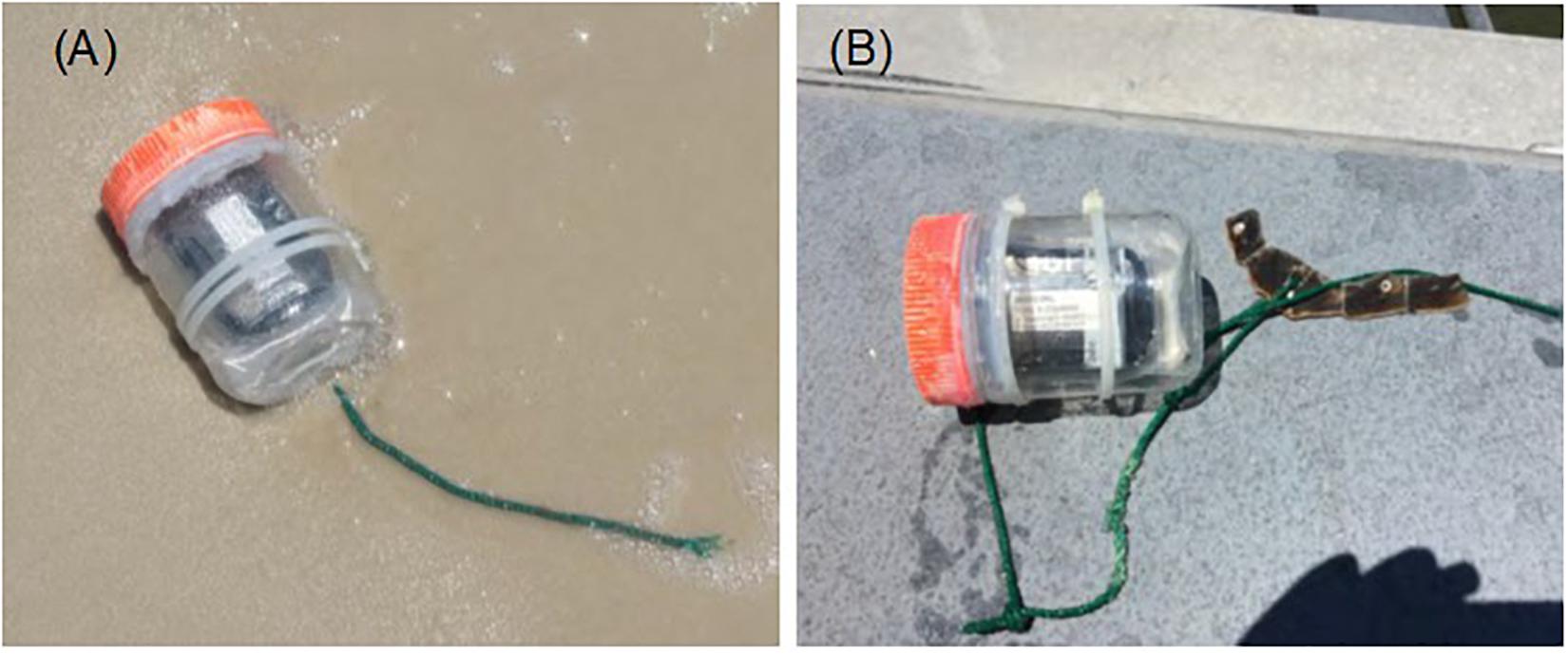
Figure 3. (A) Example of beached jar with the twine still attached but broken prior to where a carcass was attached. These carcasses are presumed to have been scavenged prior to the jar beaching. There are no instances where a jar broke free from an effigy. (B) Example of beached jar with a portion of the rear carapace remaining attached to the twine. These carcasses are presumed to have decomposed prior to the jar beaching.
Once objects reached the beach, they were located as quickly as possible to evaluate whether the carcass or effigy were still attached to the SPOT tag. If the carcass was still attached, it was photographed and the decomposition code was evaluated using the same scale as the pre-deployment classifications (Reneker et al., 2018). The second portion of the study was to determine the proportion of strandings that were reported by the public to the STSSN. Therefore, all study carcasses that beached were left in place after initial documentation. In addition, we removed the SPOT tag and twine at the time of discovery, whenever possible, to minimize any influence on later discovery or reporting. Local STSSN participants were notified of the location of the carcass as well as its unique identification number. If the carcass was subsequently reported to the STSSN by the public, the date and time of the call were recorded. If reported multiple times, authorized individuals removed the carcasses from the beach.
Water temperature at the surface and seafloor as well as surface current and wind speed at sites A–E were obtained from the Northern Gulf of Mexico Operational Forecast System (NGOFS) to investigate the seasonal variations of environmental conditions of the study region. NGOFS is a three-dimensional model that provides hourly wind, currents, water temperature and salinity over the northern Gulf of Mexico continental shelf (Wei et al., 2014). NGOFS grid resolution ranges from 10 km on the open ocean boundary to ∼600 m near the coast. The NGOFS sea surface temperature and wind at the five sites were compared with in situ observations collected during the 2017 deployments to evaluate modeling data. Both model temperature and wind were concurrent with observations. The modeled and observed wind magnitudes were generally on the same order and direction, the difference was mostly less than ± 45°. A 40 h low-pass Lanczos filter was applied to wind and current data to remove any high frequency oscillations with periods shorter than 40 h (e.g., diurnal and semi-diurnal tides, near-inertial oscillations). The 40 h low-pass filtered data showed the long-term wind and current variations. Turtle carcasses and effigies were tracked as Lagrangian surface particles forced by the drifting velocity, which is a combination of wind Wu,v and surface current Cu,v in the east (u) and north (v) direction in the north central Gulf of Mexico (Nero et al., 2013). The drifting velocity Uu,v was estimated using a similar formula as in Nero et al. (2013):
The second term on the right-hand side of the equation is the apparent wind forcing Wu,v−Cu,vadjusted by a leeway drift coefficient K. The leeway coefficient K ranged from 0.02 to 0.05, and the average value of 0.035 was used for K in this study as suggested by Nero et al. (2013).
Generalized linear mixed models (GLMM) were used to estimate the binomial probability (of drifting carcasses and effigies) to beach by season and deployment site. Two separate models were run. The first utilized a combination (n = 263) of carcasses and effigies. To maximize comparability of effigies and carcasses, only effigies with drift durations that did not exceed observed carcass decomposition rates were selected. Maximum drift durations were calculated monthly for all beached carcasses and effigies. Any effigy drift duration that exceeded the maximum carcass drift duration for that month was excluded from the analysis. The second GLMM only included carcasses (n = 163). In both instances, all deployments from sites D and E were excluded because deployments did not occur monthly. Additionally, all transmissions lost within ≤5 h were removed. Season was divided into four periods of interest that characterize the typical seasonal variation in strandings for the study area: winter pre-season (January–February), spring peak (March–June), summer lull (July–September), and fall pulse (October–December). Season, deployment site (A,B, or C) and object type (carcass or effigy) were examined as fixed effects in the model utilizing both carcasses and effigies, but only season and deployment site effects were examined for the carcass only model. Individual carcasses and effigies within a deployment event were treated as replicates. A Type III Test of Fixed Effects (alpha = 0.05) was used to test for significant effects of season, deployment site and object type. Binomial probabilities by season and site location were based on predicted marginal means (Searle et al., 1980). Multiple comparisons in the differences of estimated marginal means among seasons and deployment sites were tested at an alpha = 0.05 with a Tukey–Kramer correction. The GLMM models, estimated marginal means and multiple comparison tests were implemented using the GLIMMIX procedure in the SAS/STAT component of SAS, version 9.4 (SAS Institute Inc., Cary, NC, United States).
Deployments were conducted from January–December 2017. Over the course of 26 trips, 297 objects, 182 carcasses (61%; Figure 4A) and 115 effigies (39%; Figure 4B) were released. Over half (53%) of the objects deployed beached (n = 156). Beached objects were comprised of 41% (n = 64) sea turtle carcasses and 59% (n = 92) effigies. The remaining 47% (n = 141) of objects that did not beach were primarily sea turtle carcasses (84%, n = 118); only 16% (n = 23) of effigies did not beach. The fate of these objects included 23% of carcasses (n = 46) and effigies (n = 23) classified as unknown because either the SPOT stopped transmitting, the SPOT battery life expired while still drifting, or we were unable to recover the object. Forty percent (n = 72) of SPOT tags attached to carcasses beached without the sea turtle attached or with only part of the shell remaining; this did not occur with effigies. Based on the condition of twine, we suspect 62 were scavenged and 10 detached due to decomposition. Figure 5 shows the outcome summary of all objects deployed over the 12-month period, and the Supplemental depicts monthly deployment results. The carcasses and effigies that beached drifted for an average of 3.7 days (range: 0.4–14.6 days) and travelled an average of 86.1 km (range: 9.4–411.8 km). The longest drift track, 411.8 km, of a beaching object was from an effigy deployed at site B in August. Over the course of 13.1 days, it drifted east toward Orange Beach, AL then drifted west and beached on Horn Island, MS. Although over half of deployed objects beached, where they beached was greatly impacted by the geography of the nGOM. Nearly half (49%, n = 76) of beached objects were located on barrier islands off MS (n = 62), LA (n = 12), or AL (n = 2). Only 28% (n = 43) of beached effigies and carcasses were found on mainland beaches, primarily in MS (n = 38). Four effigies beached in AL and one effigy beached in Pensacola, Florida. The remaining 23% of objects came ashore within remote marsh areas of MS (n = 10), LA (n = 26), and AL (n = 1) and would likely never be discovered if they were an actual stranded sea turtle.
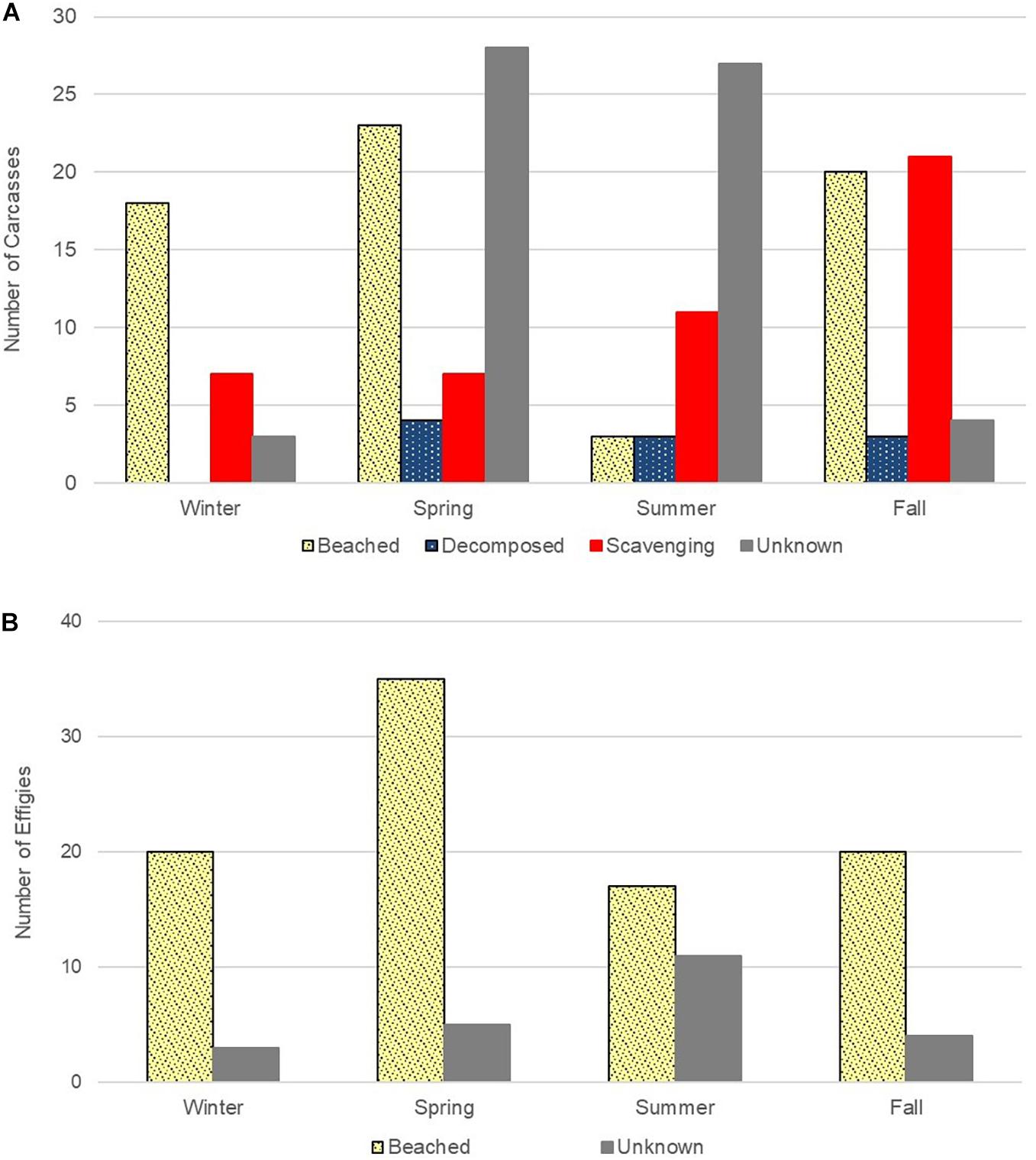
Figure 4. (A) Sea turtle carcass (n = 182) and (B) wood effigy (n = 115) outcome results by season. Both carcasses and effigies beached (n = 64 and n = 92, respectivly). Carcass (n = 46) and effigy (n = 23) outcomes were classified as unknown if the SPOT stopped working (n = 21), the SPOT battery life expired (n = 24) while still drifting, or we were unable to recover the object (n = 10). Only carcasses were decomposed (n = 10) or scavenged (n = 62).
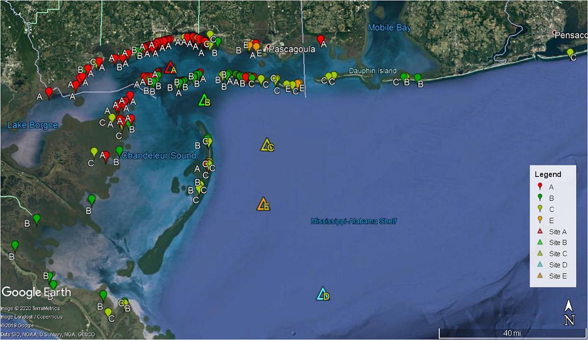
Figure 5. Locations of beached sea turtle carcasses (n = 64) and effigies (n = 92) color coded by release site (triangles). The effigy that beached on Timbalier Island, LA is not shown.
Deployment site greatly influenced if and where objects eventually beached; as distance from shore increased, the likelihood of objects beaching greatly decreased. Also, as distance from mainland MS beaches increased the likelihood of carcass scavenging also increased (Figure 5 and Table 2). Out of a total of 156 beached objects, 46% (n = 71) were from site A, 31% (n = 48) from site B, 20% (n = 31) from C, and 4% (n = 6) from E. Site A is closer to both Cat and Ship Islands (6 and 8 km, respectively) than Gulfport, MS (11 km). Although the barrier islands were closer, 42% (n = 30) of objects deployed from site A beached on the MS mainland and 31% (n = 22) beached on the MS barrier islands, followed by 17% (n = 12) beaching in northeastern LA marshes. Objects released from site A beached in all three MS coastal counties, but the majority beached in central Harrison County. Just over half (54%, n = 26) of objects deployed at site B beached on Cat, Ship, and Horn Islands. Objects from site B also beached in all three MS counties (10%, n = 5), the MS marsh (4%, n = 2), and on AL beaches (4%, n = 2). Although the Chandeleur Islands are only 11 km south of site B, only 8% (n = 4) of objects beached there. However, 19% (n = 9) beached farther west in the marshes of northeastern LA and the MS River Delta. Objects deployed at site C had the largest geographical drift distribution. Only a third of objects (n = 31) deployed from site C beached, 65% (n = 20) of them beached on nGOM barrier islands. In MS, objects were found on Ship Island, Horn Island, and Petit Bois Islands. Site C deployment objects also beached on Dauphin Island, AL, the Chandeleur Islands and one effigy drifted around the MS River Delta and beached on Timbalier Island, LA. This effigy, deployed in June, beached on Timbalier Island, LA after 6.2 days and a 359 km drift track. The only object to beach in Florida was an effigy released from site C in February; it drifted for 10 days and washed up on Pensacola Beach. Results from offshore sites D and E indicated that objects beyond approximately 100 km south of MS are very unlikely to drift northward to MS beaches or barrier islands. No effigies from site D (71 km from the closest point of land) beached; all six drifted over the continental shelf for 27 days before the SPOT batteries died. However, 67% of the effigies deployed at site E (68 km from mainland MS) beached on MS barrier islands and MS marshes. Although site E is only ∼29 km from the Chandeleur Islands, no effigies beached there.
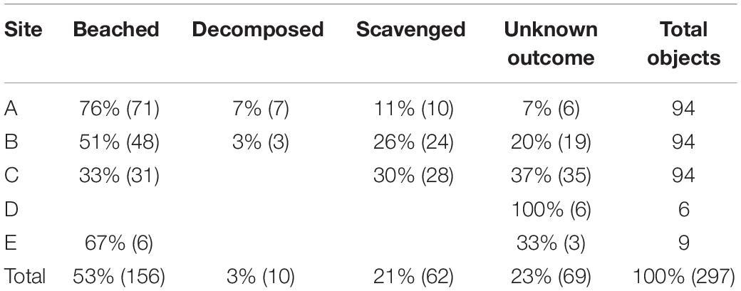
Table 2. Final outcomes of sea turtle carcasses and effigies deployed at sites A, B, C, D, and E in the northern Gulf of Mexico during 2017.
Deployment site (P ≤ 0.0001) had a significant effect on GLMM estimates of beaching probability for the model examining both sea turtle carcasses and effigies. Beaching probabilities while accounting for the significant covariates of season (P ≤ 0.0001) and object type (P = 0.0011) varied among deployment sites with probability decreasing the further offshore an object was released (Figures 2, 6). Beaching probability at deployment site A (M = 0.80, SE = 0.07) was significantly higher than at site B (M = 0.48, SE = 0.10) and site C (M = 0.17, SE = 0.06), and beaching probability was also significantly higher at site B than site C. Deployment site (P ≤ 0.0001) was also found to have a significant effect on GLMM estimates of beaching probability for the model examining only sea turtle carcasses. Beaching probability when accounting for the significant covariate of season (P = 0.0008) indicated a similar decrease in probability with distance from shore as did the model utilizing carcasses and effigies (Figure 6). Beaching probability at deployment site A (M = 0.71, SE = 0.09) was significantly higher than at site B (M = 0.26, SE = 0.09) and site C (M = 0.12, SE = 0.06). However, unlike the model utilizing turtles and effigies the probability of beaching was not significantly different between at sites B and C.
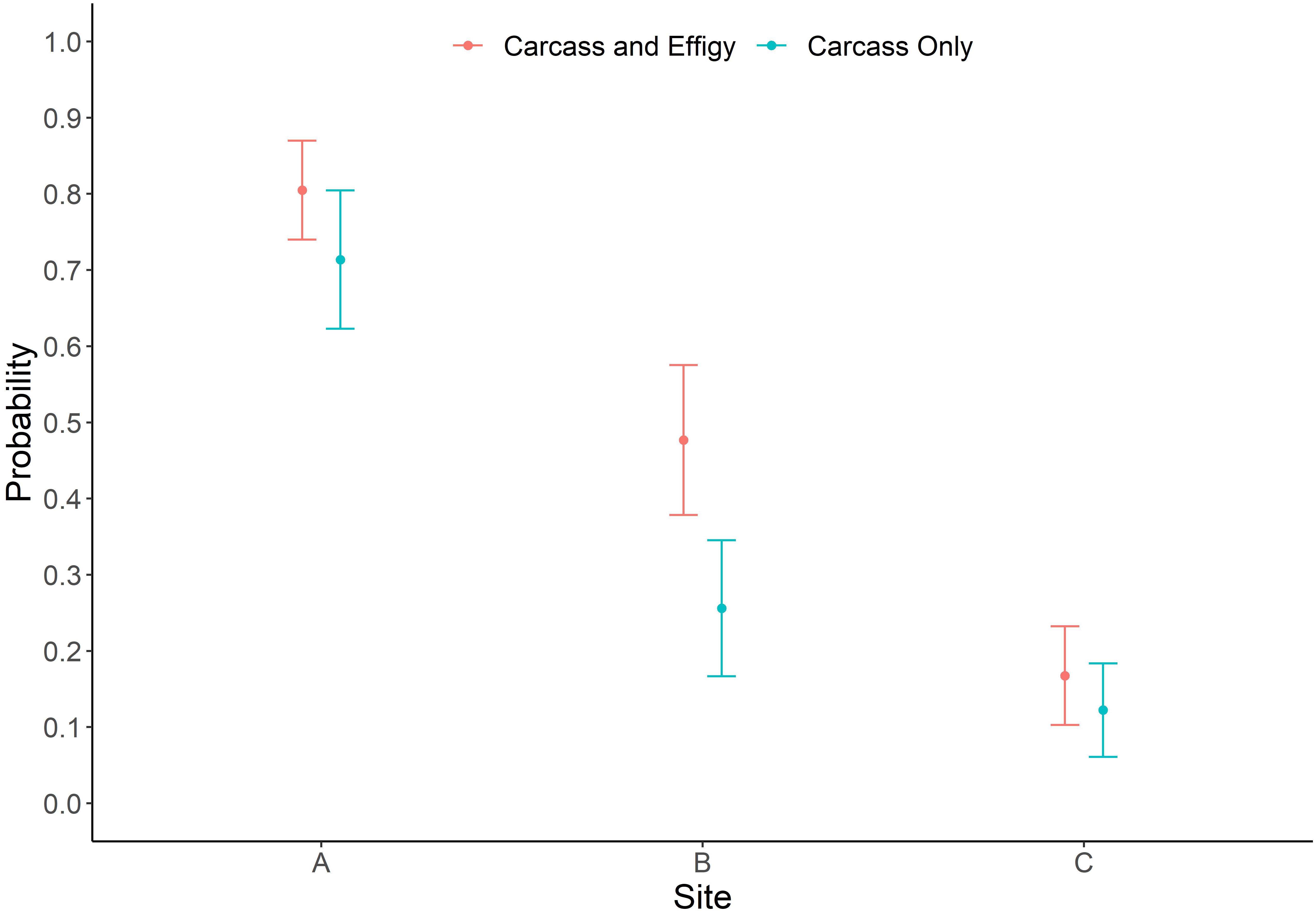
Figure 6. Probability of beaching by deployment site (A,B, and C) ± 1 standard error for carcass and effigy and carcass only models.
Object type (P = 0.0011) was found to have a significant effect on beaching probability. Effigies (M = 0.62, SE = 0.08) had a higher probability of beaching than carcasses (M = 0.33, SE = 0.07). Since effigies cannot be scavenged or decompose, effigies sometimes had considerably longer drift tracks than carcasses deployed at the same time and location, especially during summer months. Overall, effigies that eventually beached traveled an average of 96 km and 94 h (site E excluded). Beached carcasses averaged 61 km drift tracks over an average of 73 h per deployment. Although six of nine effigies deployed from site E beached, they likely did not all represent actual carcass behavior. During April deployments, the three effigies beached within 72–94 h, which overlapped the drift times (72–97 h) of the five sea turtle carcasses that also beached. In May, all three site E effigies beached within 266–272 h, while only one sea turtle carcass beached after only 94 h adrift.
Testing the effectiveness of effigies as a proxy for sea turtle carcasses was one goal of this study. Notably, carcasses and effigies had very similar drifting patterns in the nGOM. During numerous deployments, their drift tracks mirrored each other (Figure 7) and they often beached in close proximity and within hours or minutes of each other. For example, objects released at site A on April 25, 2017 drifted an average 18.7 km and all beached within 2.7 h of one another (Supplementary Figure 4). During the same trip, two of the effigies released at site E beached within a minute of each other and drifted 93.8 and 94.2 km. Similar patterns were observed offshore at site C where an effigy and two carcasses had nearly identical tracks, beaching ∼140 m apart within 38 min of each other (Supplementary Figure 2) on one of the Chandeleur Islands, LA. The separation of objects deployed at the same site and time was influenced by the intensity of the horizontal eddy diffusivity. In the examples above, the horizontal eddy diffusivity must be small to keep the objects following similar trajectories. In general, the longer the objects drifted, the further apart from each other they usually beached (Supplementary Figures). Both effigies and carcasses also tended to follow similar inertia circles due to the Coriolis Effect, which were reflected in the motions of the objects (e.g., Supplementary Figure 7).
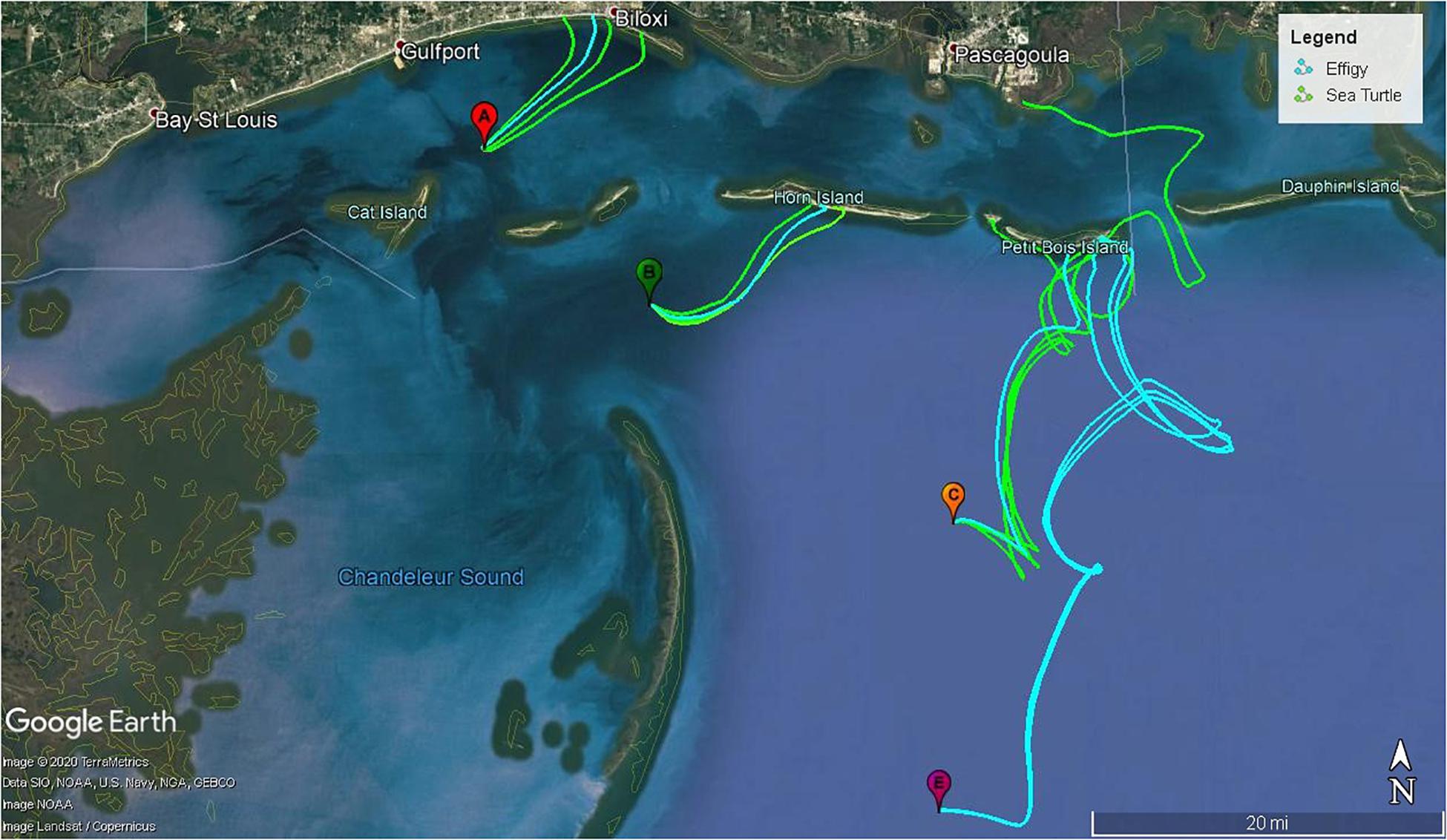
Figure 7. Carcass (green) and effigy (blue) drift tacks from sites A, B, C and E deployed on 25 April 2017. All objects beached on or before 29 April 2017.
Environmental conditions mainly have two impacts on carcasses during their drifting on the sea surface. The combination effect of wind and current drive the movement of the carcasses and determines the drifting trajectories and final stranding destinations. The sea surface temperature impacts the decomposition rate with faster decay rate under higher temperature conditions. In Figures 8, 9, we show the water temperature (A), wind (B), current (C), and wind and current combined drifting velocity (D) from NGOFS model at site A and C in 2017, respectively. Site A is an inshore station, while Site C represents the ocean conditions offshore.
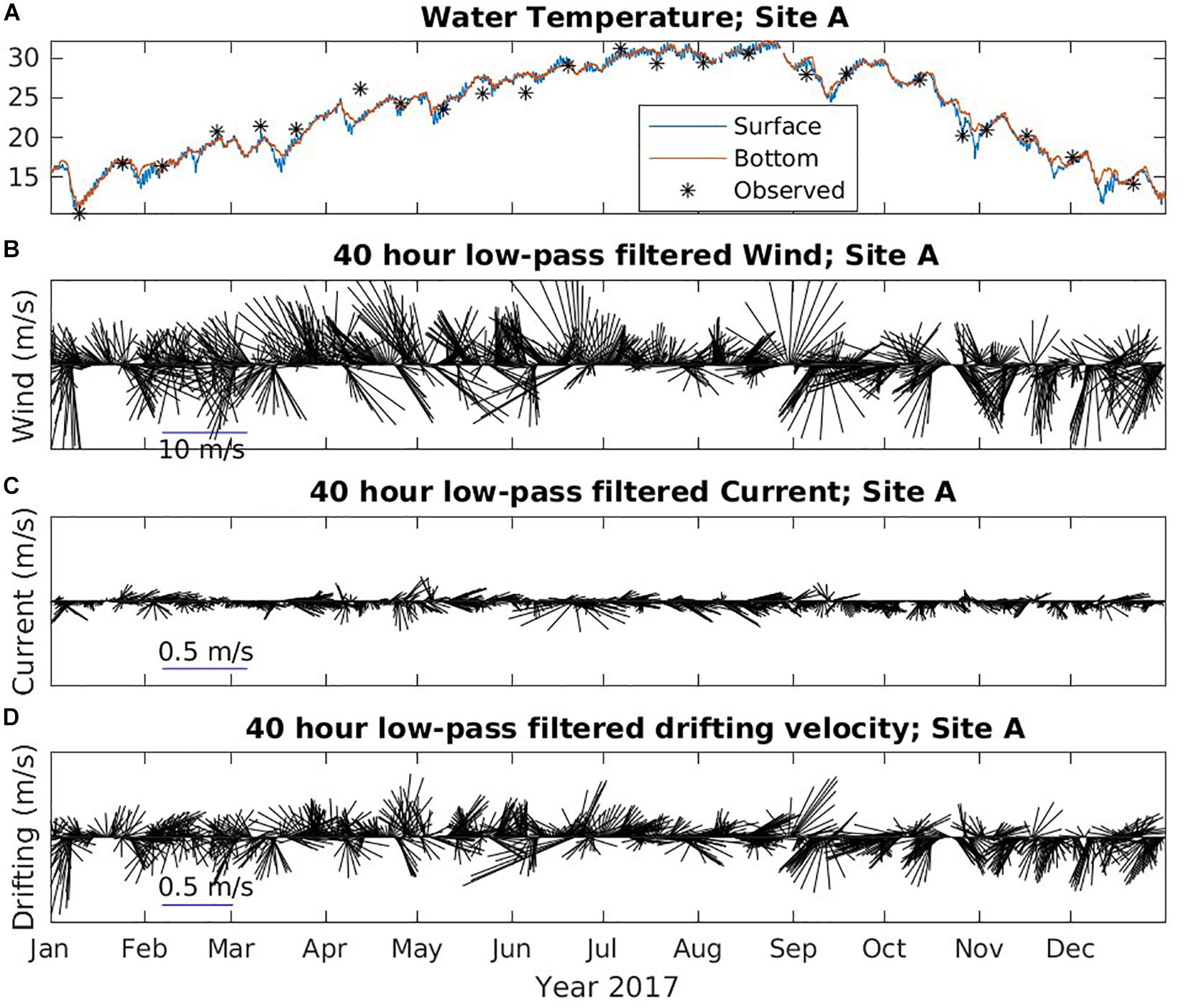
Figure 8. Time series of environmental data at Site A from NGOFS. (A) Water temperature (°C); (B) Wind vector (m/s); (C) Surface current vector (m/s); and (D) drifting velocity vector (m/s). A 40-h low-pass filter was applied to wind, current, and drifting velocity to remove the fluctuations with periods less than 40 h. Vectors pointing “up” indicate northward flow.
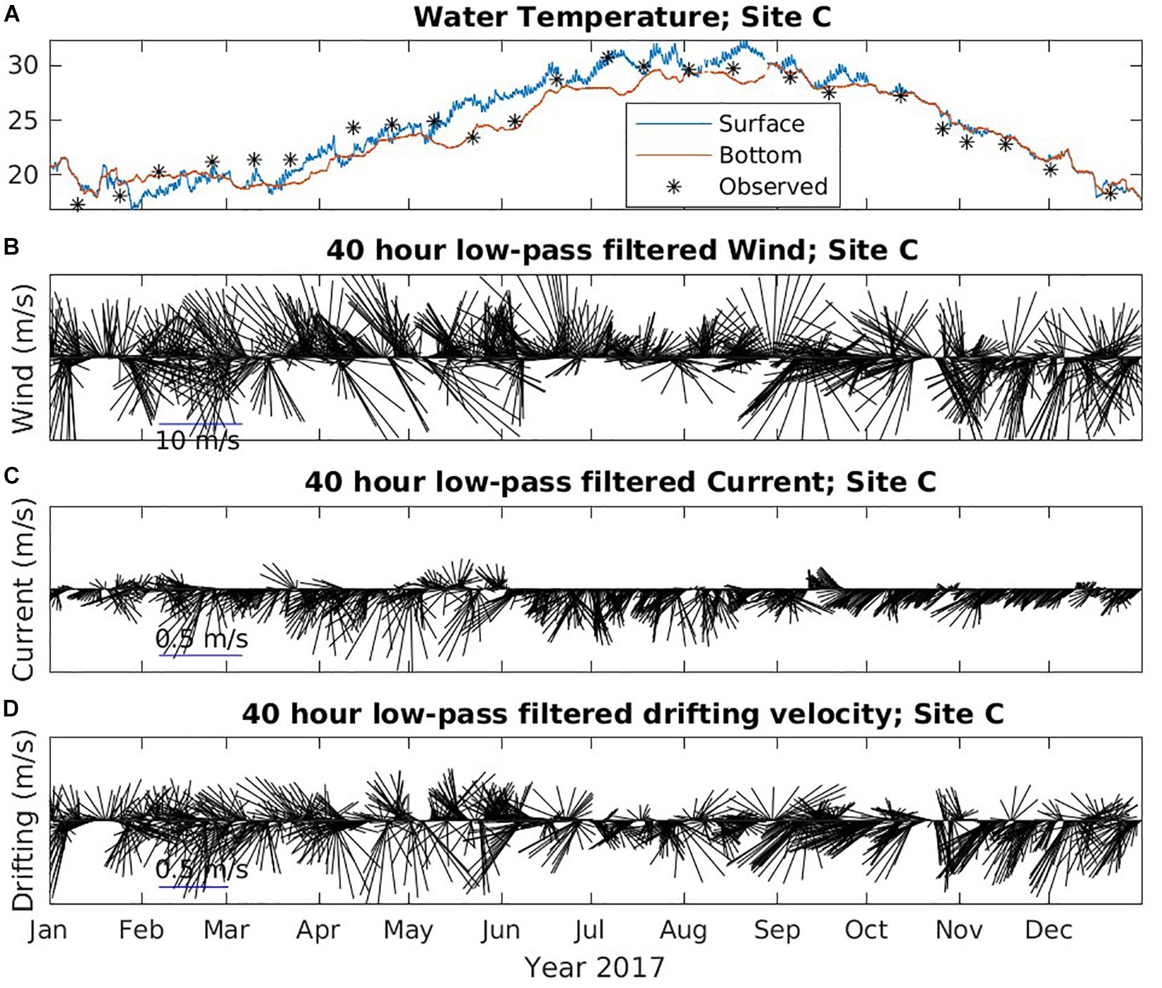
Figure 9. Time series of environmental data at Site C from NGOFS. (A) Water temperature (°C); (B) Wind vector (m/s); (C) Surface current vector (m/s); and (D) drifting velocity vector (m/s). A 40-h low-pass filter was applied to wind, current and drifting velocity to remove the fluctuations with periods less than 40 h. Vectors pointing “up” indicate northward flow.
The modeled temperature agreed reasonably well with the observed temperature in Figure 8A, suggesting model temperature could be used to investigate the seasonality in the study region. Due to the shallow depth, the inshore water at Site A was well mixed throughout 2017 indicated by the small difference between surface and bottom temperature (Figure 8A). The coolest temperature (∼13.5°C) was obtained in mid-January and the highest temperature (∼31°C) appeared in July and August at Site A. The offshore water temperature at Site B, C and E all showed similar trends and patterns. The water was well mixed and steady at approximately 20°C between January and early March. GOM waters started to warm and became weakly stratified starting in mid-March when the weather began to warm (Figure 9A). The water continued warming between April and July and enhanced stratification until the water became well mixed again in mid-September. The offshore water at Site C in general was warmer in the winter than the inshore water.
The wind vectors at all five sites followed similar patterns, though the offshore wind magnitude was slightly larger than the inshore wind (Figures 8B, 9B). The wind was stronger in fall (October–December) and winter (January–February) than in late spring (March–May) and summer (June–September). During winter, there was no obvious dominant wind direction. Wind direction could switch between onshore and offshore in hours to days. From March through the end of August, the dominant wind direction was onshore, though it changed to offshore occasionally. The wind mostly blew offshore between September and December. The water surface current at site A was small (∼0.1 m/s) and mostly along shore direction (Figure 8C). In contrast, the current at site C was much stronger and mainly toward offshore direction throughout the year (Figure 8C). The magnitude of current at site C during spring and summer is larger than fall and winter. The current at site B was also small. Site D and E had similar strong offshore current as Site C.
Due to the weak current, the direction of the drifting velocity at site A (Figure 9D) and B followed similar patterns as the wind. The drifting of surface objects was dominated by wind nearshore. Therefore, from mid-March to the end of August, the drifting was mainly northward, toward the mainland. This might explain why, although the barrier islands were closer to Site A, more objects (42%) stranded on the mainland than on the barrier islands (31%). At Site C, in fall and winter, the drift velocity had similar direction as wind suggesting that wind predominantly influenced drift. Moreover, current became weaker in fall and winter at Site C (Figures 9B,C). During spring and summer, the current and wind were generally in opposite directions. The current was strongest in the spring, while the wind was also strong. Combined drifting velocity could be onshore or offshore. In the summer, wind became weaker, but offshore current was still relatively strong. In most cases, the direction of drifting velocity followed current direction (Figure 9), suggesting current was the dominant influence in the summer at site C. Because wind and current were opposite during summer, the drift velocity tended to be the smallest among all seasons. The wind at Site D and E was similar to Site C, but the current was stronger and directed offshore, which resulted in an offshore drift. Besides the long distance to land, the strong offshore directional current might also contribute to the low stranding rate at Site D and E. We assume that fine-scale drift was more complicated than we infer because both wind and current might have changed once an object moved away from the deployment location.
Actual sea turtle strandings during 2017 (n = 66) were below the annual average based on the previous 5 years (n = 153) but followed the expected aforementioned seasonal trend [STSSN (see text footnote 1)]. Our study carcasses exhibited a similar pattern (Figure 10). Season (P ≤ 0.0001) was found to have a significant effect on GLMM estimates of beaching probability for the model examining both sea turtle carcasses and effigies (Table 3). Beaching probability, while accounting for the significant covariates of deployment site (P ≤ 0.0001) and object type (P = 0.0011), was highest during the spring and lowest during the summer (Figure 11). Beaching probability during the summer (M = 0.08, SE = 0.04) was significantly lower than winter (M = 0.90, SE = 0.06), spring (M = 0.50, SE = 0.09) and fall (M = 0.48, SE = 0.11). The probability of beaching was also significantly lower during the spring and fall than during the winter, but not significantly different between spring and fall. Season (P ≤ 0.0008) was also found to have a significant effect on GLMM estimates of beaching probability for the model examining only sea turtle carcasses (Table 3). Beaching probability, when accounting for the significant covariate of deployment site (P = 0.0003), showed a similar pattern to the model utilizing both turtles and effigies (Figure 11). Beaching probability during the summer (M = 0.04, SE = 0.03) was significantly less than winter (M = 0.80, SE = 0.11), spring (M = 0.37, SE = 0.10) and fall (M = 0.40, SE = 0.12). However, differences in beaching probability among winter, spring and fall were not significant.
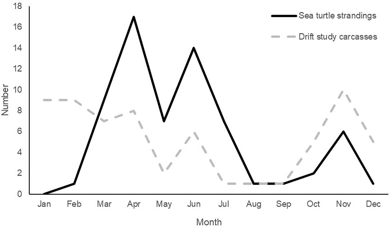
Figure 10. Number of documented sea turtle strandings (n = 66) and drift study carcasses (n = 51) that beached in Mississippi in 2017. Stranding data from the Mississippi Sea Turtle Stranding and Salvage Network database (https://grunt.sefsc.noaa.gov/stssnrep/).
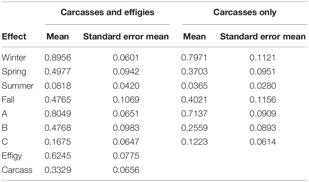
Table 3. Estimated least square means of beaching probability by season [winter pre-season (January–February), spring peak (March–June), summer lull (July–September), and fall pulse (October–December)], deployment site (A,B, or C) and object type (effigy, n = 100 or carcass, n = 163).
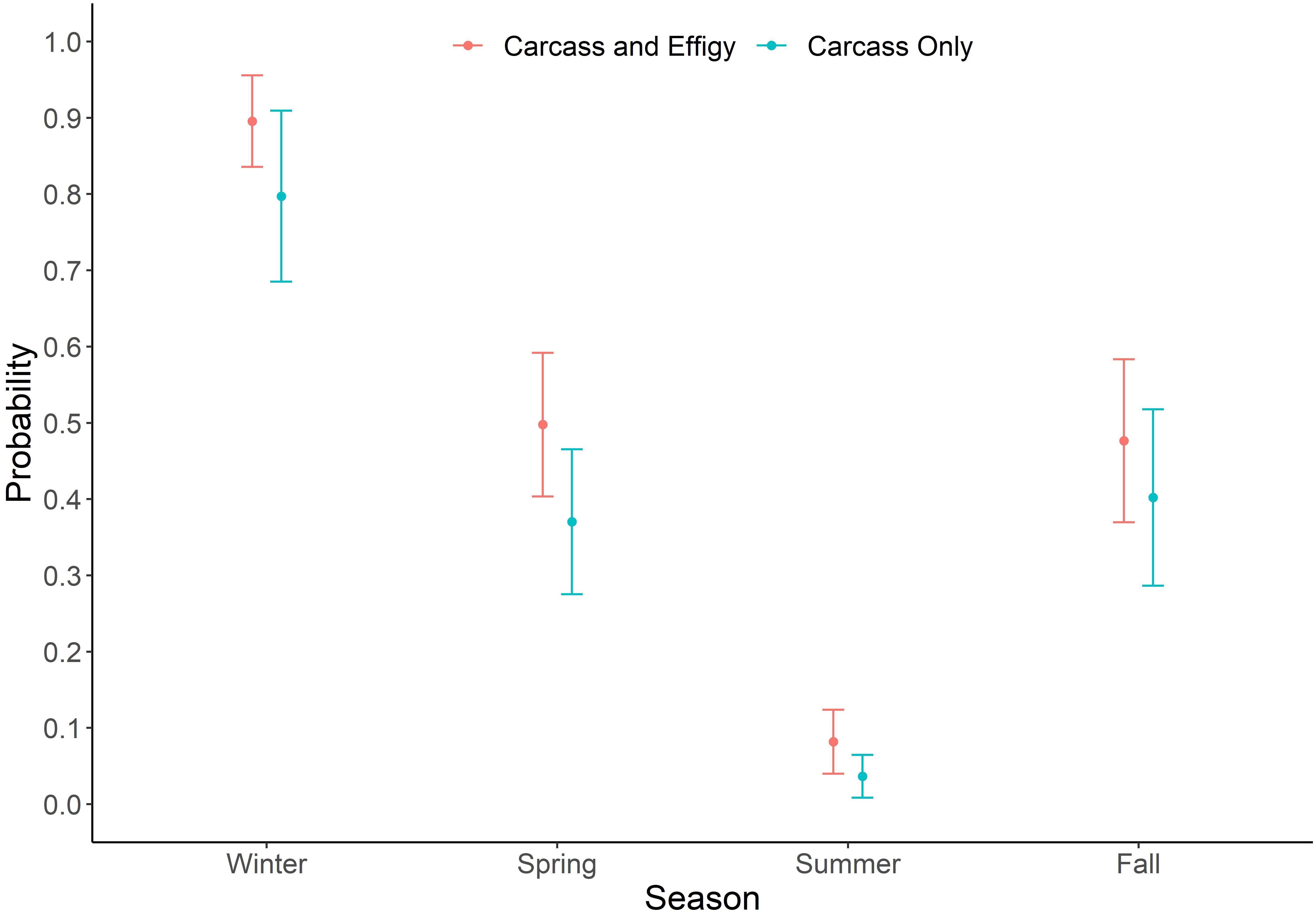
Figure 11. Probability of beaching by season ± 1 standard error for carcass and effigy and carcass only models.
Deployment site, season and environmental conditions are all factors that contribute to the stranding seasonality observed in this study (Table 4). Overall beaching probability ranges include results from both carcasses (n = 163) and effigies (n = 100) combined and carcasses only released at sites A, B and C. We attribute the significant differences between objects to lower persistence of carcasses since drift tracks and travel times were similar. Results of scavenging and decomposition apply to carcasses only. During winter, 88% of objects beached (Supplementary Figures 1, 2). No carcasses were lost due to decomposition and probable scavenging was observed in 13% of carcasses deployed in winter. Recorded surface water temperatures at deployment averaged 15.9–19.2°C, in January and February, respectively. Additionally, during winter months, greater differences in temperature were noted among sites, with colder temperatures documented inshore, e.g., 13.5°C at site A compared to 17.7°C at site C in January. Beached objects drifted for an average of 58.6 km (range: 12.5–214.0 km) and travelled an average of 3.0 days (range: 0.5–10.6 days). Overall, stranding probability was highest in winter (80–90%) than any other time of year.
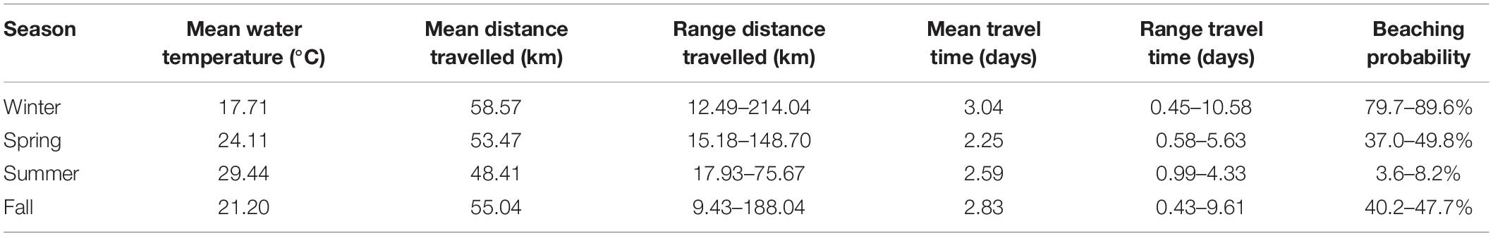
Table 4. Summary of seasonal mean water temperature, distance travelled and time traveled for beached objects [carcasses (n = 64) and effigies (n = 56)] by season [(January–February), spring (March–June), summer (July–September), and fall (October–December)]. Beaching probability ranges include results from both carcasses (n = 163) and effigies (n = 100) combined (higher values) and carcasses only released at deployment sites (A,B, and C).
In March, when strandings typically begin to occur, (Supplementary Figure 3), water temperatures began to warm and became nearly uniform between sites (21.0–21.4°C). In the following months, surface water temperatures at all sites increased to ∼27°C by June. Of the 90 objects deployed during spring, 58% beached (Supplementary Figures 4–6). The objects drifted for an average of 53.5 km (range: 15.2–148.7 km) and travelled an average of 2.3 days (range: 0.6–5.6 days). Probable scavenging of carcasses increased considerably to 47% and 7% of carcasses decomposed before beaching. Stranding probability during the peak stranding season dropped substantially following winter and was only 37–50%.
Summer surface water temperature averaged 29.4°C at all sites. Only 31% of the 64 objects deployed in summer beached (Supplementary Figures 7–9), including only three of 39 carcasses. Drift distance decreased slightly, averaging 48.4 km (range: 17.9–75.7 km), and drift duration was an average of 2.6 days (range: 1.0–4.3 days). Probable scavenging peaked at 69% during summer months, and decomposition was documented in 8% of deployed carcasses. Stranding probability dropped to 4–8% during summer months.
Surface water temperatures decreased in the fall from ∼24°C in October to ∼17°C in December. The cooler water temperatures likely contributed to the observed increase in object beaching (up to 61%) and predicted stranding probability of 40–48%. Beached carcasses were less decomposed than those observed during the summer months. Although more carcasses beached, they had similar drift durations to those that beached in late spring. During the fall, objects had the shortest drift distance and time. Objects beached in an average of 2.8 days (range: 0.4–9.6 days) (Supplementary Figures 10–12). Carcasses drifted an average of 55.1 km (range: 9.4–188.1 km). Loss of carcasses attributed to decomposition and scavenging were 7% and 10% of the documented outcomes, respectively. Unknown object outcomes were highest in fall (29%), because many of the objects drifted southwest and either never beached or came ashore along the marshlands of the eastern MS River Delta and were not recoverable.
The final portion of the study was to determine what percent of the 64 beached carcasses were reported to the STSSN in MS and adjacent states. Only 34.4% of carcasses beached on MS mainland beaches, while 40.6% of carcasses washed up on the MS barrier islands. Carcasses also beached on the LA barrier islands (4.7%), primarily the Chandeleur Islands, and the LA marshes (14.1%). Only 4.7% and 1.6% of carcasses beached in the MS and AL marshes, respectively. The MS STSSN (see text footnote 1) received 37 stranding reports for 23 carcasses from this study; several of the reports were for the same carcass. While every effort was made to remove the SPOT tags as soon as the carcasses beached or just after sunrise, it was not always possible, especially for the barrier islands and remote locations, where it took us an average of 138 h to reach them after they came ashore. However, we were successful in arriving at carcasses on the MS mainland within an average of 7 h after beaching (range: 0–27 h). As a result, SPOT tags and twine had been removed from carcasses for 25 of the public reports and 12 carcasses still had the tags attached when they were reported. There was only a 21.5% reporting rate for all beached carcasses, which can be attributed to the low reporting rate of carcasses that beached on the barrier islands and in marshes (Table 5). None of the carcasses that beached on the LA barrier islands or any of the MS, AL, and LA marshes were reported. Only 50.0% of carcasses from MS mainland beaches and 11.1% of sea turtle carcasses from the MS barrier islands were reported.
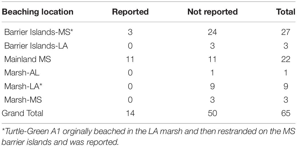
Table 5. Location and public reporting of drift study carcasses that beached in Mississipi (MS), Alabama (AL), and Louisiana (LA) during 2017. Several carcasses were reported more than once.
Numerous factors must come together for a sea turtle carcass to beach and be reported to a stranding network. First, the mortality must occur close enough to shore to allow environmental and oceanic conditions to move the carcass toward the beach. Second, the carcass must persist in the environment long enough to make it to shore and not decompose or be scavenged. Next, the carcass must beach in an area that is publicly accessible and frequently accessed. Finally, the public must be aware that sea turtle strandings should be reported and know the mechanism for doing so. This study was the first to examine how all these factors contribute to sea turtle mortality documented by a stranding network. Our results provide evidence and a plausible explanation for the annual pattern of strandings observed in MS and, likely, other nGOM states. We demonstrate that the likelihood of a sea turtle carcass beaching is significantly impacted by the time of year, environmental conditions, and proximity to shore. Moreover, similar to previous studies in other regions, our findings also show that a relatively low proportion of sea turtles that die at sea are subsequently documented as beached strandings.
On average, approximately 80% of sea turtle strandings in MS occur during March through June, with a peak in April. The proportion of carcasses we deployed during this study that came ashore mirrored the actual seasonal trend in stranding numbers during 2017, which was similar to previous years [STSSN (see text footnote 1)]. We observed that as the waters began to warm, fewer carcasses beached and losses attributed to scavenging and decomposition began to increase. During the spring peak in strandings, only 37–50% of objects are predicted to beach. Strandings begin to decline throughout June due to changing environmental conditions, such as increased water temperatures and calm winds. However, we observed a spike in beached study carcasses in June that deviated from this expected trend. Notably, this spike corresponded with an unusual number of actual sea turtle strandings (see text footnote 1). These anomalies are attributable to Tropical Storm (TS) Cindy that impacted the nGOM in June 2017. Our second June deployment occurred on 19 June, just days before TS Cindy brought strong onshore winds (Figure 8B) and increased sea states to the waters off MS. All objects from this deployment beached within 3 days of release; four were dislodged from their original beached location in the LA marsh and washed ∼120 m inland. Two effigies originally beached on Cat Island within 24 h of deployment but refloated due to TS Cindy and both beached a second time, within an hour of each other, on the mainland in Long Beach, MS (Figure 12). A second striking observation from this event was, that despite high winds and tumultuous sea state from a TS, both of the effigy tracks were nearly identical and they beached within 1.1 km of each other. This opportunistic observation highlights the impacts tropical storms may have on sea turtle strandings and the likelihood of public reporting. None of the carcasses deployed during TS Cindy were reported to the STSSN, likely a result of carcasses being pushed farther inland and absence of people on MS public beaches.
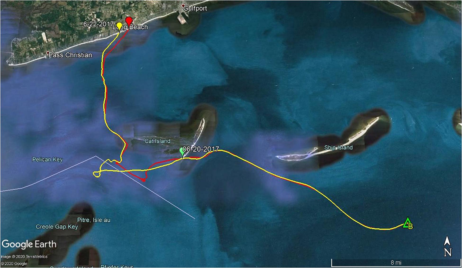
Figure 12. Effigy tracks from 25 June 2017 site B deployment. Two effigies originally beached on Cat Island within 24 h of deployment but refloated due to Tropical Storm Cindy and both beached a second time, within an hour of each other, on the mainland in Long Beach, MS.
Summer stranding probability was only 4–8%, which explains the low number of strandings documented by the MS STSSN during summer months. The two largest biological factors impeding a drifting sea turtle carcass from eventually beaching are decomposition and scavenging (or predation if the turtle is still alive), both of which follow similar temporal trends in the nGOM. Sharks are known to prey on sea turtles and scavenge sea turtle carcasses (Heithaus et al., 2008; Delorenzo et al., 2015). Both live and dead stranded sea turtles are often observed with shark bites. Stacy et al. (2021) found that 79% of shark wounds observed on a sub-set of dead stranded sea turtles from the GOM and eastern FL occurred postmortem. Although none of our carcasses beached with apparent shark bite wounds, we are considering that tags recovered with damaged tether or shark bites likely reflect scavenging of the carcass by sharks. The nGOM is a shark nursery area and habitat to adult and juvenile sharks (Parsons and Hoffmayer, 2007; Bethea et al., 2014). The area contains a diverse number of shark species including Atlantic sharpnose, Rhizoprionodon terraenovae, blacktip shark Carcharhinus limbatus, finetooth shark, C. isodon and bull shark, C. leucas (Parsons and Hoffmayer, 2007; Bethea et al., 2014). We observed predation highest in spring and fall which coincides with the movement of shark species migrating in and out of coastal MS waters (Parsons and Hoffmayer, 2005).
Another peak in beached carcasses from this study was recorded in November (n = 10) and was concurrent with a small peak in actual sea turtle strandings (see text footnote 1) (n = 6), which is typical for winter based on stranding data from prior years. This trend may reflect decreased water temperatures, which slow decomposition (Santos et al., 2018). Fall stranding probabilities, 40–48%%, are similar to those of spring. One reason the stranding numbers are likely not as high as in the spring is because sea turtles begin to migrate to warmer offshore waters as the temperature drops in the fall (Lyn et al., 2012). Also, study results and environmental conditions suggest that if sea turtles die while they are migrating out of MS waters, they will drift southwest and end up offshore or in LA marshes and never be discovered. Only sea turtles that die nearshore in the fall are likely to strand on MS mainland beaches.
Stranding location greatly affects whether sea turtles are discovered and reported. The nGOM is a diverse habitat comprised of mainland beaches, bays, bayous, marshes and barrier islands. According to NOAA,2 of the 30 United States’ states with shorelines, LA (12,426 km) is the third largest, AL (977 km) ranks 21st and MS (578 km) is 24th. MS only has 100 km of mainland shoreline, which includes only 42 km of sandy beaches3. Much of the northern GOM shoreline comprises remote habitat that is not frequented by the public. Therefore, carcasses that strand there will likely never be reported. Our study found that up to a third of carcasses beach in these remote areas. When carcasses strand, they usually remain in the same location as they initially beach. However, high tide and storm events can cause carcasses to drift and float to other locations. We observed such translocation in early March when a carcass beached in the LA marsh, where the SPOT was removed, but was reported as a stranding on West Ship Island, MS 10 days later. Translocation of stranded turtles from their original stranding site appears to be relatively rare in this region and if it does happen, carcasses are likely to be highly decomposed once they beach again.
Strandings are one of few direct methods by which we identify and monitor threats to sea turtle populations. It is possible to use location data from stranded carcasses to backtrack the carcass’s drift path to the likely area of the initial mortality (Nero et al., 2013). Backtracking can occur for individual carcasses or a combination of strandings to determine if there are specific areas of concern. Results from our drift study deployments were used to test improvements made to the model created by Nero et al. (2013). The new model now also incorporates water depth and decomposition state in addition to the previously included environmental conditions. A manuscript detailing decomposition study results, backtracking equations and drift study comparisons is currently in review.
Data derived from stranded sea turtles are frequently used for various types of research. Such valuable applications are only possible if carcasses are detected soon after discovery, i.e., with sufficient time to be located and examined. The stranding network in MS, as in many other areas, largely relies on members of the public to report stranded sea turtles. The 22% stranding reporting rate for carcasses deployed in this study was much lower than anticipated. Since the 2010 Deepwater Horizon oil spill, the MS STSSN has undertaken efforts to enhance stranding reporting within MS through public outreach, television and social media broadcasts, coordination and training of stranding response organizations and volunteers, and regimented reporting. While the MS STSSN receives reports from both the mainland beaches and offshore barrier islands, ∼80% come from the highly trafficked inland beaches. This study clearly shows that sea turtles strand along the offshore barrier islands at a comparable rate to the mainland. However, due to their relative remoteness, only a small fraction of these strandings are documented. Based on these findings, additional effort is needed to increase stranding detection and reporting on barrier islands, such as through dedicated stranding surveys or greater encouragement of opportunistic reporting by those travelling to these areas. Furthermore, the stranding reporting rate on mainland beaches was only 50%, which was also much lower than anticipated. Local organizations should enhance efforts to educate the public on what to do if they find a stranded sea turtle and seek out ways to increase public awareness, such as posting signs with stranding reporting information and through the media.
Our methods are applicable to studies of stranding probability and detection in other regions. We acknowledge that using sea turtle cadavers can be challenging and infeasible for various reasons, thus we incorporated easily fabricated effigies into our study design and demonstrate their value as a valid surrogate. By using actual carcasses, we were able to study persistence in the environment, a key variable in stranding probability; however, factors such as decomposition rates also can be inferred based on experimental studies and temperature (Cook et al., 2020). We also demonstrated a surprisingly low rate of reporting of carcasses that landed on beaches that we know are visited regularly by beachgoers. In general, structured stranding networks with established reporting mechanisms within developed areas tend to assume a relatively high rate of reporting by the public. Our findings caution against making such assumptions without having some empirical measure. We anticipate that comparable studies in other regions would have similar benefits with regard to understanding stranding patterns and trends, monitoring sources of sea turtle mortality, and evaluating the efficacy of stranding detection and reporting.
The raw data supporting the conclusions of this article will be made available by the authors, without undue reservation.
Ethical review and approval was not required for the animal study because we only used carcasses so it was not necessary. This study was authorized under United States Fish and Wildlife Service permit number TE 676395-5. No live animals were killed or harmed for this study.
MC, RN, and BS contributed to conception and design of the study. MC, JR, and RN conducted fieldwork. MC wrote the first draft of the manuscript. DH and ZW conducted environmental and statistical analysis. JR, DH, and ZW wrote sections of the manuscript. All authors contributed to manuscript revision, read, and approved the submitted version.
This research was supported with Sea Turtle Early Restoration Project funds administered by the Regional Trustee Implementation as part of the Deepwater Horizon Natural Resource Damage Assessment. This study was also partially supported by NCEI and NOAA grant 363541-191001-021000 (Northern Gulf Institute) at Mississippi State University.
JR was employed by the company Riverside Technology, Inc.
The remaining authors declare that the research was conducted in the absence of any commercial or financial relationships that could be construed as a potential conflict of interest.
We would like to thank the staff and volunteers from the Massachusetts, Texas, and North Carolina Sea Turtle Stranding and Salvage Networks for salvaging carcasses, especially R. Prescott and K. Dourdeville from Massachusetts Audubon Wellfleet and K. Sampson, M. Godfrey, and S. Finn for authorizing carcass use and shipping carcasses. Without their dedication and response effort, this study would not have been possible. We would also like to thank the NOAA MS Laboratory staff, especially the NOAA Gear Monitoring Team for their help in deployment and recovery efforts and E. Schultz for reviewing the manuscript. The model data is from the Northern Gulf of Mexico Operational Forecast System (NGOFS) hosted at NOAA National Centers for Environmental Information (NCEI): https://www.ncei.noaa.gov/thredds/model/ngofs_catalog.html.
The Supplementary Material for this article can be found online at: https://www.frontiersin.org/articles/10.3389/fmars.2021.659536/full#supplementary-material
Bethea, D. M., Ajemian, M. J., Carlson, J. K., Hoffmayer, E. R., Imhoff, J. L., Grubbs, R. D., et al. (2014). Distribution and community structure of coastal sharks in the northeastern Gulf of Mexico. Environ. Biol. Fishes 98, 1233–1254. doi: 10.1007/s10641-014-0355-3
Caillouet, C. W., Shaver, D. J., Teas, W. G., Nance, J. M., Revera, D. B., and Cannon, A. C. (1996). Relationship between sea turtle stranding rates and shrimp fishing intensities in the northwestern Gulf of Mexico: 1986-1989 versus 1990-1993. Fishery Bull. 94, 237–249.
Casale, P., Affronte, M., Insacco, G., Freggi, D., Vallini, C., d’Astore, P., et al. (2010). Sea turtle strandings reveal high anthropogenic mortality in Italian waters. Aquat. Conserv. 20, 611–620. doi: 10.1002/aqc.1133
Coleman, A. T., Pitchford, J. L., Bailey, H., and Solangi, M. (2016). Seasonal movements of immature Kemp’s ridley sea turtles (Lepidochelys kempii) in the northern gulf of Mexico. Aquat. Conserv. 27, 253–267. doi: 10.1002/aqc.2656
Cook, M., Reneker, J. L., Nero, R. W., Stacy, B. A., and Hanisko, D. S. (2020). Effects of freezing on decomposition of sea turtle carcasses used for research studies. Fishery Bull. 118, 268–274. doi: 10.7755/FB.118.3.5
Delorenzo, D., Bethea, D., and Carlson, J. (2015). An assessment of the diet and trophic level of Atlantic sharpnose shark Rhizoprionodon terraenovae. J. Fish Biol. 86, 385–391. doi: 10.1111/jfb.12558
Epperly, S. P., Braun, J., Chester, A. J., Cross, F. A., Merriner, J. V., Tester, P. A., et al. (1996). Beach strandings as an indicator of at-sea mortality of sea turtles. Bull. Mar. Sci. 59, 289–297.
Foley, A. M., Stacy, B. A., Schueller, P., Flewelling, L. J., Schroeder, B., Minch, K., et al. (2019). Assessing Karenia brevis red tide as a mortality factor of sea turtles in Florida, USA. Dis. Aquat. Organ. 132, 109–124. doi: 10.3354/dao03308
Hart, K. M., Mooreside, P., and Crowder, L. B. (2006). Interpreting the spatio-temporal patterns of sea turtle strandings: going with the flow. Biol. Conserv. 129, 283–290. doi: 10.1016/j.biocon.2005.10.047
Heithaus, M. R., Wirsing, A. J., Thomson, J. A., and Burkholder, D. A. (2008). A review of lethal and non-lethal effects of predators on adult marine turtles. J. Exp. Mar. Biol. Ecol. 356, 43–51. doi: 10.1016/j.jembe.2007.12.013
Koch, V., Peckham, H., Mancini, A., and Eguchi, T. (2013). Estimating at-sea mortality of marine turtles from stranding frequencies and drifter experiments. PloS One 8:e56776. doi: 10.1371/journal.pone.0056776
Lyn, H., Coleman, A., Broadway, M., Klaus, J., Finerty, S., Shannon, D., et al. (2012). Displacement and site fidelity of rehabilitated immature Kemp’s ridley sea turtles (Lepidochelys kempii). Mar. Turt. Newsl. 135, 10–13.
Mancini, A., Koch, V., Seminoff, J. A., and Madon, B. (2011). Small-scale gill-net fisheries cause massive green turtle Chelonia mydas mortality in Baja California Sur. Mexico. Oryx 46, 69–77. doi: 10.1017/S0030605310001833
Nero, R. W., Cook, M., Coleman, A. T., Solangi, M., and Hardy, R. (2013). Using an ocean model to predict likely drift tracks of sea turtle carcasses in the north central Gulf of Mexico. Endanger. Species Res. 21, 191–203. doi: 10.3354/esr00516
Parsons, G. R., and Hoffmayer, E. R. (2005). Seasonal changes in the distribution and relative abundance of the Atlantic sharpnose shark Rhizoprionodon terraenovae in the north central Gulf of Mexico. Copeia 2005, 914–920. doi: 10.1643/0045-8511(2005)005[0914:scitda]2.0.co;2
Parsons, G. R., and Hoffmayer, E. R. (2007). Identification and characterization of shark nursery grounds along the Mississippi and Alabama gulf coasts. Am. Fish. Soc. Symp. 50, 301–316.
Reneker, J. L., Cook, M., and Nero, R. W. (2018). Preparation of Fresh Dead Sea Turtle Carcasses for at-Sea Drift Experiments. NMFS-SEFSC- Vol. 731, Pascagoula, MS: U.S. Department of Commerce, 14. doi: 10.25923/9hgx-fn38
Santos, B. S., Kaplan, D. M., Friedrichs, M. A. M., Barco, S. G., Mansfield, K. L., and Manning, J. P. (2018). Consequences of drift and carcass decomposition for estimating sea turtle mortality hotspots. Ecol. Indic. 84, 319–336. doi: 10.1016/j.ecolind.2017.08.064
Searle, S. R., Speed, F. M., and Milliken, G. A. (1980). Population marginal means in the linear model: an alternative to least squares means. Am. Stat. 34, 216–221. doi: 10.2307/2684063
Shaver, D. J. (1991). Feeding ecology of wild and head-started Kemp’s ridley sea turtles in south Texas waters. J. Herpetol. 25, 327–334. doi: 10.2307/1564592
Shoop, C. R., and Ruckdeschel, C. (1982). Increasing turtle strandings in the southeast United States: a complicating factor. Biol. Conserv. 23, 213–215. doi: 10.1016/0006-3207(82)90076-3
Stacy, B. A. (2014). Summary of Necropsy Findings for Non-Visibly Oiled Sea Turtles Documented by Stranding Response in Alabama, Louisiana, and Mississippi 2010 Through 2014. DWH Sea Turtles NRDA Technical Working Group Report. NOAA-NMFS. NOAA Technical Report DWH-AR0149557. NOAA-NMFS, 133.
Stacy, B. A., Foley, A. M., Shaver, D. J., Purvin, C. M., Howell, L. N., Cook, M., et al. (2021). Scavenging versus predation: shark-bite injuries in stranded sea turtles in the southeastern USA. Dis. Aquat. Org. 143, 19–26. doi: 10.3354/dao03552
Keywords: carcass drift, carcass decomposition, sea turtle strandings, endangered species, stranding seasonality, stranding reporting rates, sea turtle effigies
Citation: Cook M, Reneker JL, Nero RW, Stacy BA, Hanisko DS and Wang Z (2021) Use of Drift Studies to Understand Seasonal Variability in Sea Turtle Stranding Patterns in Mississippi. Front. Mar. Sci. 8:659536. doi: 10.3389/fmars.2021.659536
Received: 27 January 2021; Accepted: 06 April 2021;
Published: 16 June 2021.
Edited by:
Donna Jill Shaver, National Park Service, United StatesReviewed by:
Marc Girondot, Université Paris-Sud, FranceCopyright © 2021 Cook, Reneker, Nero, Stacy, Hanisko and Wang. This is an open-access article distributed under the terms of the Creative Commons Attribution License (CC BY). The use, distribution or reproduction in other forums is permitted, provided the original author(s) and the copyright owner(s) are credited and that the original publication in this journal is cited, in accordance with accepted academic practice. No use, distribution or reproduction is permitted which does not comply with these terms.
*Correspondence: Melissa Cook, bWVsaXNzYS5jb29rQG5vYWEuZ292
Disclaimer: All claims expressed in this article are solely those of the authors and do not necessarily represent those of their affiliated organizations, or those of the publisher, the editors and the reviewers. Any product that may be evaluated in this article or claim that may be made by its manufacturer is not guaranteed or endorsed by the publisher.
Research integrity at Frontiers
Learn more about the work of our research integrity team to safeguard the quality of each article we publish.