Seasonal Evolution of Cape Darnley Bottom Water Revealed by Mooring Measurements

This study examines the seasonal evolution of Cape Darnley Bottom Water (CDBW), using the results of mooring and hydrographic measurements in the slope region off Cape Darnley in 2008–2009 and 2013–2014. Newly formed CDBW began reaching the western and nearshore part of the slope region off Cape Darnley in April, spread to the offshore and eastern part in May, and reached the easternmost part in September. The potential temperature and salinity decreased and the neutral density increased when newly formed CDBW reached mooring sites. Potential temperature-salinity properties of CDBW changed over time and location. The salinity of the source water of CDBW estimated from potential temperature-salinity diagrams started to increase at a nearshore mooring in late April, which is about 2 months after the onset of sea-ice production, and continued to increase during the ice production season. It is most probable that the accumulation of brine in the Cape Darnley polynya produces the seasonal variation of potential temperature-salinity properties of CDBW. Two types of CDBW were identified. Cold and less saline CDBW and warm and saline CDBW were present in Wild and Daly Canyons, respectively. This indicates that the salinity of the source water of CDBW increased in the westward direction. CDBW exhibited short-term variability induced by baroclinic instability.

1. Introduction

Antarctic Bottom Water (AABW) is the major source of the bottom water of the world ocean. AABW spreads directly into the Atlantic Ocean and, in a modified form as the denser part of the Lower Circumpolar Deep Water (LCDW), into the Pacific and Indian Oceans, forming the lower cell of the meridional overturning circulation (Mantyla and Reid, 1983; Orsi et al., 1999). The formation of AABW enhances the exchange of heat and fresh water between the surface layer, which is exposed to the atmosphere, and the deep layer, which has a large volume and heat content, contributing to the maintenance of the global climate. Compared with the North Atlantic Deep Water, which is formed by the cooling of saline Atlantic Water in the Greenland and Nordic Seas, AABW is characterized by low temperature and low salinity (Mantyla and Reid, 1983) because its formation is accompanied by sea-ice production (Foster and Carmack, 1976).

Antarctic Bottom Water is formed from shelf water (SW), which is characterized by the near-freezing temperature and high salinity. High sea-ice production in polynyas on the shelf is the source of SW. SW is transformed into AABW as it descends the slope and mixes with ambient water. The Weddell and Ross Seas, which have large continental embayments with major continental ice shelves, are two distinct formation sites of AABW (Jacobs et al., 1970; Foster and Carmack, 1976). A third formation site of AABW was identified off the Adélie and George V Land coast (Rintoul, 1998), where enhanced sea-ice production in the coastal polynya directly causes the formation of SW and thus AABW (Williams et al., 2010). In addition, the fourth site for AABW formation has been speculated to exist in the eastern sector of the Weddell-Enderby Basin (Meredith et al., 2000; Meijers et al., 2010). A map the of sea-ice production estimated from satellite-derived heat flux (Tamura et al., 2008) suggested that the Cape Darnley polynya (light shaded area in Figure 1) is the site with the second–highest production of sea ice around Antarctica after the Ross Ice Shelf polynya. Ohshima et al. (2013) conducted mooring measurements off Cape Darnley and showed that newly formed AABW descends the slope and reaches the abyss. This newly formed AABW is referred to as Cape Darnley Bottom Water (CDBW).

FIGURE 1

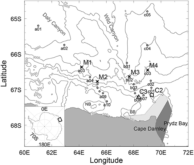
Figure 1. A bathymetry map of the study area (International Bathymetric Chart of the Southern Ocean, IBCSO: Arndt et al., 2013). Locations of moorings M1–M4 and conductivity, temperature, and depth (CTD) stations are shown by crosses and circles, respectively. The Cape Darnley polynya and grounded ice are shaded by light and dark gray, respectively. Locations of moorings C2 and C3 are shown by a square and a triangle, respectively. Transects passing stations a01–a10, b01–b07, and c01–c05 are defined as transects A, B, and C, respectively. BB and NB indicate Burton and Nielsen Basins, respectively. The thick solid line in the inset map shows the location of the study area.

In addition to the Cape Darnley polynya, several polynyas with relatively high ice production are distributed on the western (lee) side of the landfast ice or glacier tongue in East Antarctica (Nihashi and Ohshima, 2015). Among them, the Vincennes Bay polynya possibly contributes to the production of the upper layer of AABW in the East Antarctic (Kitade et al., 2014). However, based on nearly 3,000 temperature and salinity profiles from autonomous floats along the East Antarctic coast between 50 and 128°E, the region off Cape Darnley appears to be the main AABW source (Wong and Riser, 2013).

The results of a numerical experiment using a nonhydrostatic ocean model showed that SW spreads along the canyons of the slope (Nakayama et al., 2014). As it descends the slope, SW forms a westward bottom-intensified current and is transformed into CDBW mixed with the overlying modified Circumpolar Deep Water (mCDW; Hirano et al., 2015). Dense water affected by CDBW is transported westward by the Slope Current along the continental slope (Wong and Riser, 2013; Aoki et al., 2020). Couldrey et al. (2013) argued that the recent southward migration of the Antarctic Circumpolar Current enhanced the mixing of CDBW with warm mCDW in the Cape Darnley region, with the warming signal of CDBW reaching the eastern Weddell Gyre. Offshore transport of CDBW may also enhance the intrusion of mCDW into the shelf region, which may enhance the melting of ice shelves (Morrison et al., 2020).

The purpose of this study is to examine the seasonal evolution and horizontal distribution of CDBW. For this purpose, we analyze temperature, salinity, and velocity data obtained from the mooring and hydrographic measurements off Cape Darnley. We use data obtained from four moorings deployed in the slope region in 2008–2009 and two moorings deployed in the shelf region in 2013–2014 and hydrographic data obtained in 2009. Ohshima et al. (2013) provided the first evidence of the formation of CDBW, using mooring data collected in 2008–2009. They mostly investigated newly formed CDBW descending Wild Canyon, which is located just off the Cape Darnley polynya. Although it was also suggested that part of CDBW descends down Daly Canyon, which is located to the west of the Wild Canyon, the characteristics of CDBW in Daly Canyon was not examined. They also did not investigate the seasonal variation of the characteristics of CDBW. In this study, we examine the spatial variation of the characteristics of CDBW, combining results of the mooring measurements with hydrographic data obtained in broad regions including both Wild and Daly Canyons. We also examine the seasonal variation of the characteristics of CDBW. It is shown that potential temperature-salinity properties of CDBW changed with the season, because the salinity of the source water of CDBW increased with time. Thus, we examine the mechanism of the seasonal variation of potential temperature-salinity properties of CDBW, using sea ice production rate in the Cape Darnley polynya and salinity data obtained by moorings on the shelf. When CDBW arrived at mooring sites, a clear periodic variability of velocity, temperature, and salinity with the period of 3–5 days has been observed (Ohshima et al., 2013). We also examine the physical mechanism of this variability. This study is organized as follows. In section 2, we describe the mooring and hydrographic measurements. Results of these measurements are presented in section 3. In this section, we examine the seasonal evolution, horizontal distribution, and the short-term variability of CDBW. Section 4 provides a study summary and conclusions.

2. Data

Figure 1 shows the locations of the mooring sites and hydrographic stations. Four moorings, M1–M4, were deployed in February 2008–January 2009 off Cape Darnley in an extensive Japanese mooring program conducted as a part of the International Polar Year (Ohshima et al., 2013). The Cape Darnley polynya is located on the western side of the grounded iceberg tongue, which is located between 69 and 71°E. Four moorings were deployed in the north and northwest regions of the Cape Darnley polynya. Moorings M2 (bottom depth: 1,437 m) and M4 (depth: 1,824 m) were located in the upper part of the slope, whereas moorings M1 (depth: 2,923 m) and M3 (depth: 2,608 m) were located in the deeper part of Daly and Wild Canyons, respectively. To supplement results obtained from these moorings, we also analyzed temperature and salinity data obtained at two additional moorings, C2 (depth: 368 m) and C3 (depth: 355 m), which were deployed near the shelf break in 2013–2014 (Figure 1). The moorings were equipped with conductivity-temperature sensors (CT sensors; Sea-Bird SBE-37 MicroCAT), downward-looking acoustic Doppler current profilers (ADCP; Teledyne RD Instruments WorkHorse Sentinel 300), and current meters (Union Engineering RU-1, with the exception of Aanderaa RCM7 being used at mooring C3). These instruments were deployed within 300 m from the bottom (Table 1).

TABLE 1

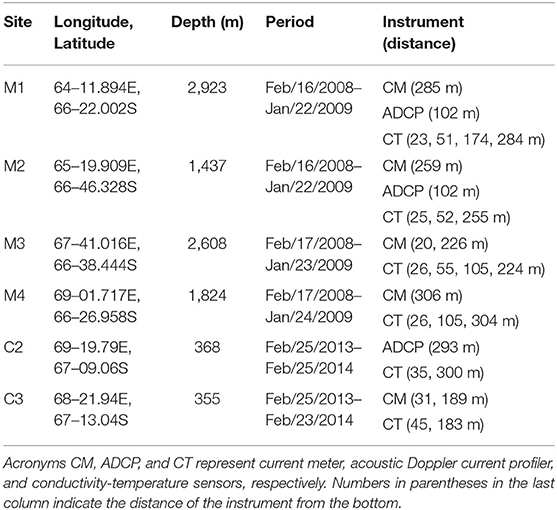
Table 1. Mooring location, bottom depth, period, and instrument.

Sampling intervals of the moored instruments were 2 h for the current meters, 1 h for the ADCPs, and 5 or 10 min for the CT sensors. We applied a Godin filter to salinity and temperature data and subsampled the filtered data at 1 h intervals. Then, we removed the tidal component from all temperature, salinity, and velocity data using a Lanczos-cosine filter (Lancz7) with a cutoff period of 34.29 h (Emery and Thomson, 2001). In contrast to the Ross Sea, where strong tides are observed (Whitworth and Orsi, 2006), the tidal current was weaker than 5 cm s⁻¹ at our mooring sites. Hence, we expect that the tidal energy included in the filtered data is negligible, even though a small amount of the energy of the O1 tidal constituent tends to be passed through a Lancz7 filter.

Hydrographic measurements were carried out along three transects when moorings M1–M4 were recovered in January 2009 (Figure 1). We defined transects A, B, and C as transects passing stations a01–a10, b01–b07, and c01–c05, respectively. The hydrographic data were obtained by TR/V Umitaka-Maru using a conductivity, temperature, and depth profiler (CTD; Sea-Bird SBE911 plus with SBE43). Conductivity (and dissolved oxygen) data were calibrated by bottle samples. We calculated neutral density, γ_n, using the method of Jackett and McDougall (1997) for both mooring and CTD measurements; however, we found that γ_n included a large uncertainty on the shelf and the upper part of the slope, as described by Williams et al. (2010). Hence, we used the potential density referenced to 2,500 dbar, σ₂₅, to compare the densities obtained at all mooring sites.

As a measure of the mass of brine rejected in the Cape Darnley polynya, we used sea-ice production estimated by the ice thickness, which was derived from the Advanced Microwave Scanning Radiometer-Earth Observing System (AMSR-E) data and a heat flux calculation (Nakata et al., 2019, 2021). We used a time series of sea-ice production in the Cape Darnley polynya, the domain of which is shown in Figure 1 of Tamura et al. (2008). In addition to the International Bathymetric Chart of the Southern Ocean (IBCSO: Arndt et al., 2013), we used bathymetry data obtained by a shipboard multi-narrow beam echo sounder (MBES; L-3 Communications ELAC Nautik SeaBeam3020) to examine the precise bathymetry around mooring M3. The bathymetry data were constructed from MBES data obtained by R/V Hakuho-Maru in 2008, 2016, and 2019 and Icebreaker Shirease in 2009–2013. The seawater sound velocity used in MBES was corrected by real-time data obtained by the surface water velocity meter and by temperature and salinity profiles obtained by CTD and expendable CTD.

3. Results

Figure 2 shows potential temperature-salinity (θ-S) diagrams for all CTD stations. The black, blue, and red lines indicate data in the offshore, slope, and shelf regions, which are defined as the regions where the bottom depth is greater than 3,000 m, between 1,000 and 3,000 m, and smaller than 1,000 m, respectively. Using this diagram, we can identify major water masses distributed off Cape Darnley, following the definitions provided by Whitworth et al. (1998). Water characterized by a near-freezing temperature and salinity higher than 34.5 was present in the shelf region. This water corresponds to SW. SW was present at stations a08, a09, and a10, which were located in a small depression on the shelf. In the offshore and slope regions, water denser than γ_n = 28.27 kg m⁻³ was present near the bottom. This water corresponds to AABW. In some studies, water denser than γ_n = 28.27 kg m⁻³ and warmer than the freezing temperature is divided into modified Shelf Water (mSW) and AABW, which are present near the shelf and in the offshore region, respectively (Orsi and Wiederwohl, 2009; Wong and Riser, 2013); however, we do not divide AABW into mSW and AABW, because many mooring sites and CTD stations were located in the slope region, in which the boundary between mSW and AABW is not clear enough. Warm deep water existing above AABW is Circumpolar Deep Water (CDW; 28.03 < γ_n < 28.27 kg m⁻³), whereas cold surface water characterized by the temperature minium is Antarctic Surface Water (AASW; γ_n < 28.03 kg m⁻³). As shown by blue and red lines, CDW was mixed with AASW and transformed into mCDW in the slope and shelf regions.

FIGURE 2

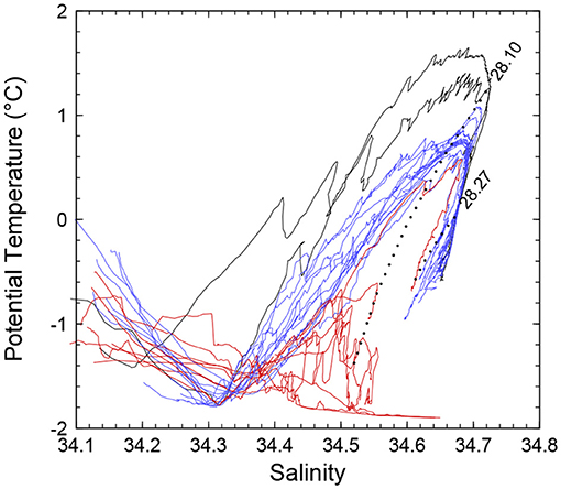
Figure 2. θ-S diagrams for all CTD stations. Black, blue, and red lines indicate data in the offshore, slope, and shelf regions. The potential temperature and salinity at depths shallower than 40 m are not shown. The dotted lines indicate the contours of γ_n.

Figure 3 shows the vertical section of potential temperature and salinity on transect B. Cold and less saline water was present along the bottom of the slope. The gray dashed lines indicate the γ_n = 28.10 and 28.27 kg m⁻³ neutral surfaces. Because γ_n exceeded 28.27 kg m⁻³, the cold and less saline water on the slope is CDBW. The γ_n = 28.27 kg m⁻³ neutral surface shoaled toward the coast, indicating that CDBW was accompanied by a westward current that intensified near the bottom (Hirano et al., 2015). The γ_n = 28.10 kg m⁻³ neutral surface was close to the maximum local temperature at offshore stations. Spreading along this neutral surface, CDW can mix with AASW near the shelf, and a front was formed between the two at the shelf break (Figure 3A). This front corresponds to the Slope Front (Whitworth et al., 1998).

FIGURE 3

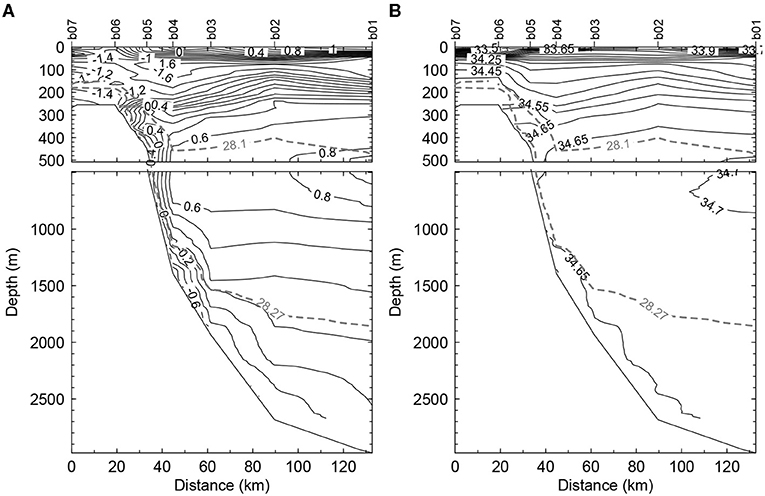
Figure 3. Contours of (A) potential temperature and (B) salinity on transect B. The gray dashed lines indicate the contours of γ_n.

3.1. General Properties of CDBW

In this section, we examine the general properties of temperature, salinity, and velocity of CDBW obtained by mooring measurements. Figure 4 shows the mean flow and standard deviation ellipses at two depths at moorings M1–M4. Here, the direction of the isobath at each mooring site is indicated by the long blue bars. The mean flow was directed westward at mooring M2, which was consistent with the direction of the Antarctic Slope Current (Meijers et al., 2010). The Antarctic Slope Current was also present at mooring M4, although the mean flow was weaker than the standard deviation there. Standard deviation ellipses were polarized (anisotropic) at moorings M2 and M3. Both the mean flow and major axis of the standard deviation ellipse were directed along the isobath at mooring M2, suggesting that the direction of the flow was restricted by bottom topography (Figure 4A). Such features were also present at mooring M3 for the bathymetry based on MBES observation (Figure 4B). As suggested in Figure 3, CDBW was accompanied by a bottom intensified current. The mean speed at mooring M3 increased from 7 cm s⁻¹ at 226 m from the bottom to 14 cm s⁻¹ at 20 m from the bottom, which was consistent with a bottom intensified current driven by CDBW.

FIGURE 4

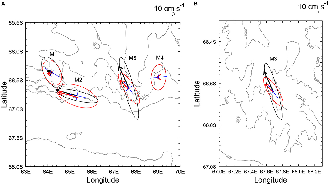
Figure 4. Vectors of the mean velocity and standard deviation ellipses in (A) the entire mooring region and (B) the region around mooring M3. The black vectors and ellipses indicate the mean velocity and standard deviation ellipses for the deepest velocity data. The red vectors and ellipses indicate the mean velocity and standard deviation ellipses for the shallowest velocity data. Contours in (A,B) indicate the isobath based on IBCSO and a shipboard MBES observation, respectively. The bathymetry was not obtained by multi-narrow beam echo sounder (MBES) in part of the region in (B). In that region, bathymetry was supplemented by the global relief model ETOPO1 (Amante and Eakins, 2009). The long and short blue bars indicate the direction parallel and normal to the isobath, respectively. The direction of the isobath at mooring M3 and other mooring sites was estimated from the bathymetry data based on shipboard MBES observation and IBCSO, respectively.

Figure 5 shows the time series of the along-isobath and across-isobath velocities for the deepest velocity data at moorings M1–M4. The along-isobath velocity increased during the period from May to November, especially at moorings M2 and M3. The temporal variability of velocity was also amplified in the same period. The along-isobath velocity at mooring M3 oscillated almost regularly at a period of 3–5 days. We will examine the mechanism of this variability in section 3.4.

FIGURE 5

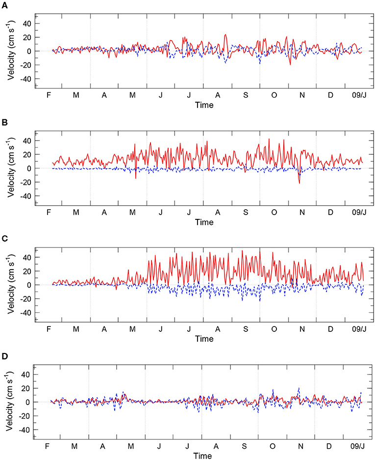
Figure 5. Time series of the along-isobath velocity, u′, (red line) and across-isobath velocity, v′, (blue dashed line) for the deepest velocity data at mooring (A) M1, (B) M2, (C) M3, and (D) M4.

Figure 6 shows the time series of potential temperature, salinity, and γ_n near the bottom at each mooring site. Potential temperature and salinity started to decrease in April at mooring M2, in May–June at moorings M1 and M3, and in September at mooring M4. With the decrease of potential temperature and salinity, γ_n increased. Since γ_n exceeded 28.27 kg m⁻³, except for April–May at mooring M2 where the uncertainty of γ_n was large, water observed at mooring sites mostly corresponds to AABW or CDBW. Thus, cold and less saline water observed at moorings M1–M4 corresponds to the newly formed CDBW, whereas warmer water corresponds to other AABW. At moorings M2 and M3, the current speed increased along with the arrival of the newly formed CDBW (Figure 5). The decrease in potential temperature and salinity was large at moorings M2 and M4 in the upper part of the slope, compared with moorings M1 and M3 in the deeper part of the slope, indicating that CDBW is modified by the mixing with ambient water as it descends the slope.

FIGURE 6

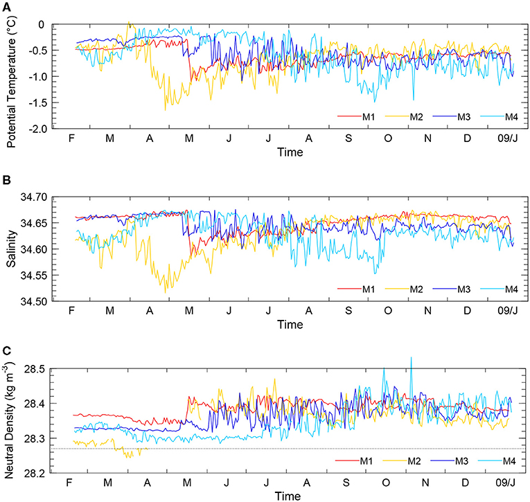
Figure 6. Time series of (A) potential temperature, (B) salinity, (C) and γ_n obtained by the deepest conductivity-temperature (CT) sensors at moorings M1 (red), M2 (orange), M3 (blue), and M4 (light blue). In (C), lines are not drawn in the period when the uncertainty of γ_n exceeds 0.03 kg m⁻³. The horizontal dotted line in (C) indicates γ_n = 28.27 kg m⁻³.

Potential temperature decreased first in April at mooring M2, which was located in the upper part of the slope; it subsequently decreased in May-June at moorings M1 and M3, which were located in the deeper part of the slope, and in September at mooring M4, which was the easternmost mooring. Thus, the potential temperature decreased earlier at moorings, which were located in the western and shallower regions. According to the laboratory and numerical experiments, when dense water forms on the shelf, geostrophic adjustment finishes shortly after the formation, and the dense water flows westward along the isobath in the southern hemisphere. Afterward, the dense water slowly spreads in the offshore direction in time and the downstream region in space (Chapman and Gawarkiewicz, 1995; Baines and Condie, 1998). The difference in the timing of the temperature decrease between moorings M1–M4 is consistent with experimental results by Chapman and Gawarkiewicz (1995) and Baines and Condie (1998). Because mooring M4 was located about 100 km north of the Cape Darnley polynya (Figure 1), dense water observed at this mooring may correspond to the newly formed AABW from Prydz Bay (Williams et al., 2016), which is located east of Cape Darnley. Williams et al. (2016) showed that newly formed AABW starts to be exported from Prydz Bay in September, which approximately coincides with the timing of temperature decrease at mooring M4. Hence, Prydz Bay may be the source of water observed at mooring M4. On the other hand, as we will show later, the characteristics of water observed at moorings M3 and M4 are similar to each other, except that the former is modified more strongly by the mixing with ambient water. Thus, both the Cape Darnley region and Prydz Bay are the possible source of newly formed AABW observed at mooring M4.

To examine the seasonal evolution of newly formed CDBW, we divided the mooring period evenly into four parts. We defined periods February 16–May 12, May 12–August 6, August 6–October 31, and October 31–January 25, 2009, as periods P1, P2, P3, and P4, respectively. The length of each period is 86 days. Figure 7 shows the vertical distribution of mean σ₂₅ in periods P1–P4 at each mooring. At moorings M1–M3, σ₂₅ near the bottom increased between periods P1 and P2, whereas σ₂₅ increased between periods P2 and P3 at mooring M4. This increase in σ₂₅ indicates the arrival of newly formed CDBW, as it was shown in Figure 6. With the arrival of newly formed CDBW, σ₂₅ increased by 0.02–0.04 kg m⁻³ at all depths except for the uppermost CT sensors at mooring M4. Newly formed CDBW was distributed within 100–300 m or more from the bottom. σ₂₅ also increased near the bottom at CTD stations near moorings M3 and M4 (solid lines in Figure 7), indicating that newly formed CDBW was present at these CTD stations.

FIGURE 7

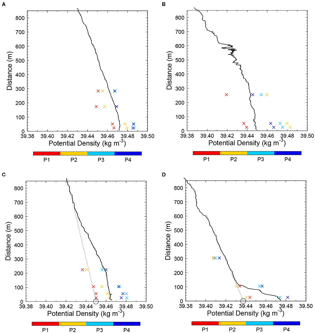
Figure 7. Seasonal variability of the vertical distribution of σ₂₅ at mooring (A) M1, (B) M2, (C) M3, and (D) M4. The vertical axis indicates the distance from the bottom. The red, orange, light blue, and blue crosses indicate mean σ₂₅ in periods P1, P2, P3, and P4, respectively. The solid lines in (A–D) indicate the vertical distribution of σ₂₅ at CTD stations, a03, a05, b02, and c03, respectively. The circles and dotted lines in (C,D) indicate values of σ_Ab and fitting lines used in section 3, respectively. The details are discussed in the text.

3.2. The Seasonal Evolution of CDBW and Its Source Water

In this section, we examine more precisely the seasonal evolution of the characteristics of CDBW. Figure 8 shows θ-S diagrams for the deepest CT sensors at each mooring. The plus signs are plotted in 1 day interval, and the color of the plus signs indicates periods P1–P4. In periods P1 and P2, data were scattered along a straight line for each mooring except for period P1 at mooring M1, indicating the mixing of two water masses. That is, it is suggested that CDBW observed at the mooring sites were formed by the mixing between cold and less saline water and warm and saline water. For the rest of this study, this line is referred to as the mixing line. At mooring M2, even though data were scattered along two different mixing lines in periods P1 and P2, the slopes of the mixing lines were similar to each other. The slopes of the mixing lines at the other three moorings were also similar to those at mooring M2. We determined the slope of the mixing line in each period for all moorings, fitting salinity and potential temperature by a linear function. The principal components regression was used for the fitting. Because the variance of salinity is much smaller than that of potential temperature, we normalized salinity and potential temperature with their standard deviation in the entire mooring period, when we calculated the regression. The slope of the mixing lines and the proportion of the variance explained by the first principal component are listed in Supplementary Table 1. The slopes of the mixing lines in periods P1 and P2 at moorings M2–M4 and in period P2 at mooring M1 were 8–11 and quite close to each other. More than 95% of the variance was explained by the first principal component for these mixing lines, indicating that data fit well to these mixing lines. Gray lines in Figures 8A–D indicate the mean slope of these mixing lines. In periods P1 and P2, data at all moorings were scattered along a line that is nearly parallel to this gray line except for period P1 at mooring M1, indicating that mixing lines at all moorings were nearly parallel to each other in these periods. This was also the case for mixing lines at shallower CT sensors (not shown).

FIGURE 8

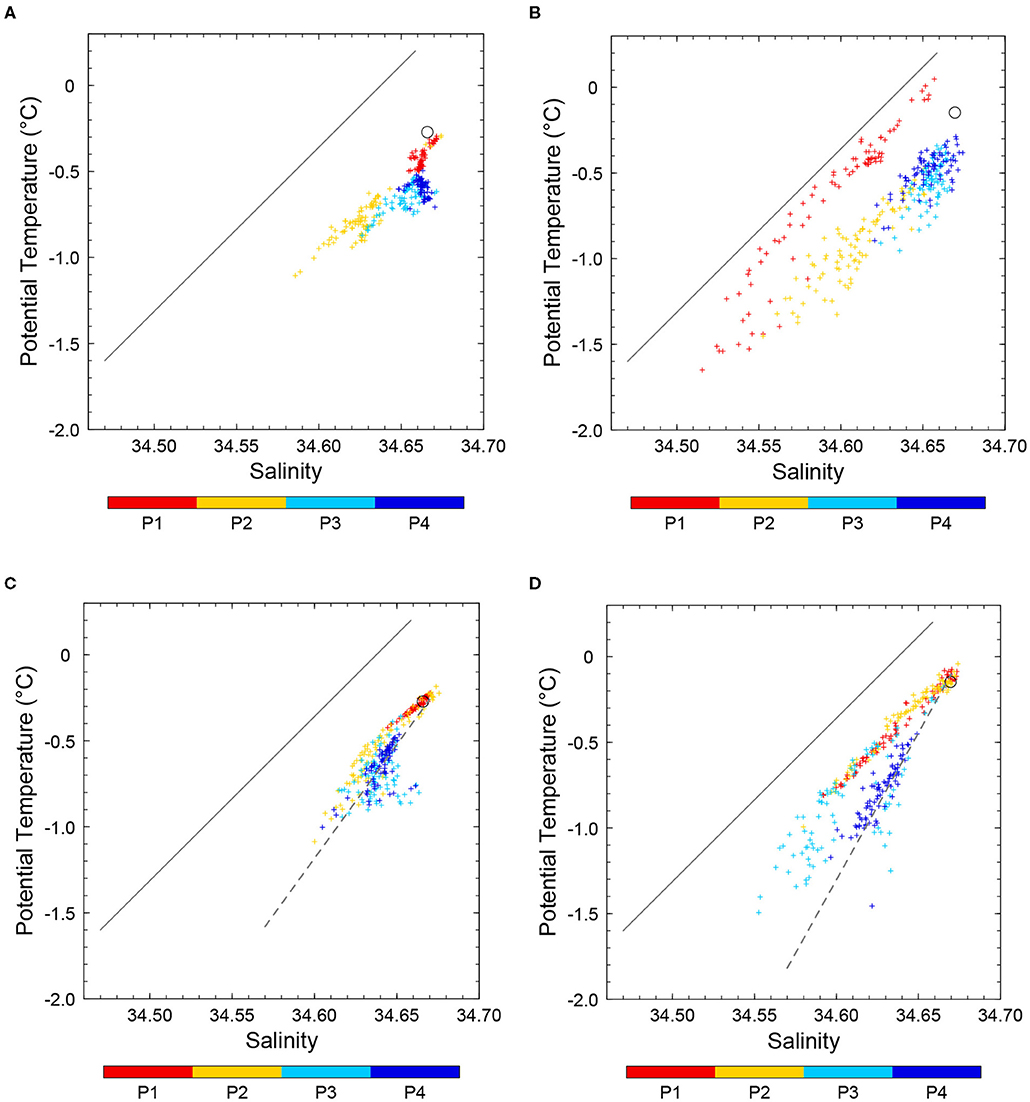
Figure 8. θ-S diagrams for the deepest CT sensors at mooring (A) M1, (B) M2, (C) M3, and (D) M4. The red, orange, light blue, and blue pluses indicate salinity and potential temperature in periods P1, P2, P3, and P4, respectively. The gray lines indicate the mean slope of the mixing line in periods P1 and P2. The gray dashed lines in (C,D) indicate the mixing line in period P4 at moorings M3 and M4, respectively. The circles indicate the point, (S, θ) = (S_Ab, θ_Ab), which is used in the Results Section. The details are discussed in the text.

At moorings M3 and M4, which were located in and upstream of Wild Canyon, respectively, data were scattered along another mixing line in periods P3 and P4. For example, gray dashed lines in Figures 8C,D indicate the mixing line in period P4 at these moorings. Since the slope of the mixing line was larger than that in periods P1 and P2, it is suggested that CDBW in periods P3 and P4 consisted of cold water with a salinity that was higher than that in periods P1 and P2. In contrast, in periods P3 and P4, CDBW observed at mooring M1, which was located in Daly Canyon, was warmer and saltier than that at moorings M3 and M4. Since potential temperature and salinity data of this warm and saline CDBW were not located along the mixing line obtained at moorings M3 and M4, the source of CDBW at the mooring M1 was likely different from that at moorings M3 and M4. Relatively warm and saline CDBW was also observed at the mooring M2, which was located upstream of Daly Canyon. Thus, cold and less saline CDBW and warm and saline CDBW were present near Wild and Daly Canyons, respectively.

Using θ-S diagrams shown in Figure 8, we estimate the salinity of source water of CDBW and examine the mechanism of the temporal and spatial variation of the characteristics of CDBW shown in Figure 8. As suggested in Figure 8, CDBW is formed by the mixing of cold and less saline water and warm and saline water. We assume that the former and the latter correspond to SW, which is the source water of CDBW, and ambient water, respectively. Then, the salinity and potential temperature of CDBW obtained by CT sensors are expressed as

$\begin{array}{ll}{S}_C=r_{SW}{S}_{SW}+(1-r_{SW})S_A& (1)\end{array}$

$\begin{array}{ll}{\theta }_C=r_{SW}{T}_f+(1-r_{SW}){\theta }_A& (2)\end{array}$

where S_C, S_SW, and S_A are salinity of CDBW, SW, and ambient water, respectively, θ_C and θ_A are the potential temperature of CDBW and ambient water, respectively, T_f is the freezing tempetature, and r_SW is the mixing ratio of SW. In Equation (2), we assumed that potential temperature of SW is T_f. Equations 1 and 2 represent the mixing line. If we know S_A and θ_A, we can calculate S_SW and r_SW from S_C and θ_C using these equations.

To obtain S_A and θ_A, we examine the vertical distribution of the potential temperature and salinity observed at all CTD stations (Supplementary Figure 1). At station c05, which was the deepest and easternmost station, the newly formed CDBW was absent, except for the thin layer near the bottom (Supplementary Figures 1E,F). Thus, we assume that S_A and θ_A are salinity and potential temperature at station c05. Thick orange lines in Figures 9A,B indicate a θ-S curve for S_A and θ_A. We can express this curve in a functional form as follows:

$\begin{array}{ll}{\theta }_A=f(S_A).& (3)\end{array}$

FIGURE 9

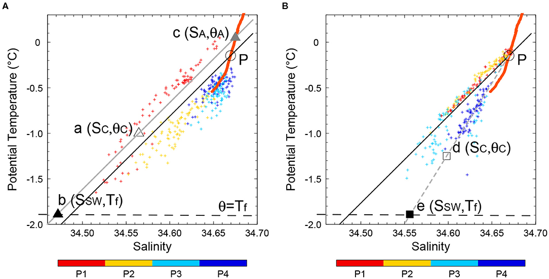
Figure 9. Schematic showing how to determine mixing lines, S_SW, S_A, and θ_A. The solid line indicates a line passing through the point P (circle). The thick orange line indicates a θ-S curve for CTD station c05. The long dashed line indicates the freezing line, θ = T_f. The gray line in (A) indicates the mixing line for CDBW located at point a (triangle). This CDBW is formed by the mixing of SW located at point b (black triangle) with ambient water located at point c (gray triangle). The dashed gray line in (B) indicates the mixing line for CDBW located at point d (square). This CDBW is formed by the mixing of SW located at point e (solid square) with ambient water located at point P. As in Figure 8B, the pluses with colors in (A,B) indicate (S, θ) data obtained by the deepest CT sensor at moorings M2 and M4, respectively. The details are discussed in the text.

The point (S, θ) = (S_A, θ_A) is located on this curve.

We assume that ambient water spreads along isopycnals and that SW is mixed with ambient water as it is transported from the shelf to the mooring sites. Since CTD station c05 is located in the deep region, the deeper part of the water at CTD station c05 cannot reach to the mooring sites. We define S_Ab, θ_Ab, and σ_Ab as salinity, potential temperature, and σ₂₅ of the most dense ambient water that can reach to each mooring site, respectively. The point P in Figures 9A,B indicate the position of (S, θ) = (S_Ab, θ_Ab) at moorings M2 and M4, respectively. SW cannot mix with ambient water below the point P. We will describe how S_Ab, θ_Ab, and σ_Ab were determined later in this section.

As shown in Figure 8, the slope of the mixing line was approximately constant in periods P1 and P2, whereas the slope of the mixing line in periods P3 and P4 was larger than that in periods P1 and P2 at moorings M3 and M4. Thus, we estimate S_SW and θ_SW by combining two different methods. The solid line in Figures 9A,B indicates a line passing through the point P. The slope of this line is the same as that of the gray line in Figure 8, that is, the mean slope of mixing lines at all moorings in periods P1 and P2. We estimate S_SW and r_SW of CDBW located in the regions above and below this line as follows. In both regions, ambient water that is mixed with SW corresponds to AABW or the deep part of CDW.

• When the point (S, θ) = (S_C, θ_C), which indicates S and θ of CDBW, is located above the solid line (Figure 9A), we assume that the mixing line is parallel to this line for simplicity, based on results shown in Figure 8. That is,

$\begin{array}{ll}s=\frac{{\theta }_C-{\theta }_A}{S_C-S_A}& (4)\end{array}$

where s is the slope of the solid line. Then, we can determine S_SW and r_SW, using Equations (1–4). For example, when the point (S_C, θ_C) is located at point a (open triangle) in Figure 9A, the gray line, which is parallel to the (black) solid line and passes through point a, corresponds to the mixing line for this CDBW. Then, point b (solid triangle), which is the crossing of the mixing line and freezing line, θ = T_f (long dashed line), corresponds to (S, θ) = (S_SW, T_f). Similarly, point c (gray triangle), which is the crossing of the mixing line and the thick orange line, corresponds to (S, θ) = (S_A, θ_A).

If point a is located below the solid line, point c is located below point P, which corresponds to (S, θ) = (S_Ab, θ_Ab) (even if such point c exists). This means that σ₂₅ of ambient water exceeds σ_Ab and contradicts the assumption. Thus, we can apply the method described here only when the point (S_C, θ_C) is located above the solid line.

• When the point (S_C, θ_C) is located below the solid line (Figure 9B), we simply assume the following:

$\begin{array}{ll}{S}_A=S_{Ab}\mathrm{\text{and}}{\theta }_A={\theta }_{Ab}.& (5)\end{array}$

Hence, the point P corresponds to the point (S, θ) = (S_A, θ_A). Then, we can determine S_SW and r_SW, substituting Equation 5 to Equations 1 and 2. For example, when the point (S_C, θ_C) is located at point d (open square) in Figure 9B, the gray dashed line, which passes through points d and P, corresponds to the mixing line for this CDBW. The slope of the mixing line is larger than the solid line, which is consistent with the results shown in Figure 8. Then, point e (solid square), which is the crossing of the mixing line and the freezing line, corresponds to (S, θ) = (S_SW, T_f).

When (S_C, θ_C) is very close to point P, the value of S_SW is sensitive to a small change in S_C and θ_C. Thus, we did not use results when r_SW < 0.05.

We determined σ_Ab from the vertical distribution of σ₂₅ at CTD stations b02 and c03, which were located near moorings M3 and M4, respectively (Figures 7C,D). At these stations, σ₂₅ increased due to the newly formed CDBW near the bottom. Dotted lines in Figures 7C,D indicate the line fitted to σ₂₅ in the layer above the newly formed CDBW. We obtained these lines fitting σ₂₅ within 600–1,000 m and 100–500 m from the bottom by the least square method for CTD stations b02 and c03, respectively. These lines approximately represent the vertical distribution of σ₂₅ that is not affected by CDBW. Then, we extrapolated these lines and defined σ_Ab as the value of σ₂₅ extrapolated to the bottom (circles in Figures 7C,D). Then, we define S_Ab and θ_Ab as values of S_A and θ_A on the isopycnal surface of σ₂₅ = σ_Ab at CTD station c05. The layers occupied by CDBW and other AABW were difficult to discriminate at moorings M1 and M2 (Figures 7A,B). Hence, we used S_Ab obtained at moorings M3 and M4 for moorings M1 and M2, respectively, because bottom depths at moorings M3 and M1 and those at moorings M4 and M2 were similar to each other. The position of (S_Ab, θ_Ab) at each mooring site is indicated by circles in Figure 8. We can verify that at moorings M3 and M4, the circles and (θ, S) data in periods P3 and P4 were approximately aligned on the same line. To examine how strongly the results of S_SW and r_SW depend on the value of S_Ab (and θ_Ab), we changed the value of S_Ab. Isopycnal surfaces σ₂₅ = σ_Ab for moorings M3 and M4 were located at depths of 2,860 and 2,424 m at CTD station c05, respectively. We substituted values of S and θ at depths 500 m shallower than these depths to S_Ab and θ_Ab, respectively. We also substituted values of S and θ just above the thin layer of CDBW near the bottom to S_Ab and θ_Ab, respectively. However, the change in S_SW and r_SW was <0.02 and 0.1, respectively. Thus, results of S_SW and r_SW do not strongly depend on the value of S_Ab (and θ_Ab).

Figures 10A,B show the time series of S_SW and r_SW, respectively. In some period in April–June, S_SW and r_SW are not shown because r_SW was <0.05. The salinity of source water of CDBW, S_SW, at mooring M1 was similar to that at mooring M2 in May–November, indicating that CDBW at moorings M1 and M2 originated from the same source. The source of CDBW at moorings M3 and M4 was less saline compared with that of CDBW at moorings M1 and M2, corresponding to lower salinity at these moorings (Figure 6B). The mixing ratio, r_SW, was higher at moorings M2 and M4, which were located in the upper part of the slope, compared with that at moorings M1 and M3, which were located in the deeper region. Thus, CDBW mixes with ambient water as it descends the slope. The mixing ratio increased in April and decreased in May at mooring M2 and increased in September and decreased in October at mooring M4, corresponding to the change in potential temperature (Figure 6A). At mooring M2, S_SW started to increase in late April. At mooring M1, S_SW started to increase about 1 month later, when S_SW at mooring M2 reached about 34.5. Because moorings M1 and M2 were located in the shallower and deeper part of the slope, respectively, it is suggested that CDBW cannot reach the deep region until salinity and density get high enough. At moorings M3 and M4, S_SW started to increase 2 and 5 months later than at mooring M2, respectively. At all moorings, S_SW continued to increase until October–November.

FIGURE 10

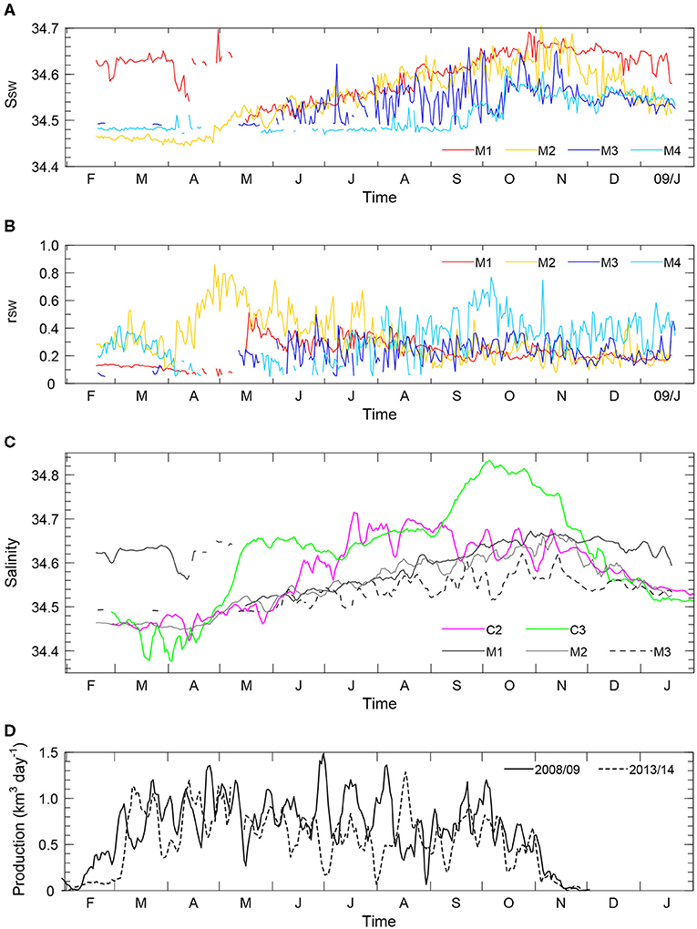
Figure 10. (A,B) Time series of (A) S_SW and (B) r_SW for the deepest CT sensors at moorings M1 (red), M2 (orange), M3 (blue), and M4 (light blue). (C) Time series of salinity at moorings C2 (magenta) and C3 (green). The solid, gray, and dashed lines in (C) indicate S_SW at moorings M1, M2, and M3, respectively. (D) Time series of sea-ice production in the Cape Darnley polynya in 2008–2009 (solid line) and 2013–2014 (dashed line). A 5 day running mean is taken for data in (C,D). The lines are not drawn for S_SW and r_SW in the period of r_SW < 0.05 in (A–C).

Figure 10C compares S_SW with salinity obtained by the deepest CT sensors at moorings C2 and C3, which were deployed at the shelf break in 2013–2014. Potential tempetature at these moorings was close to the freezing point from February to November (not shown). Thus, SW or AASW was present at these mooring sites. The value of S_SW at moorings M1–M3 approximately compares with the salinity at mooring C2 except for July–August. Sea-ice production in the Cape Darnley polynya in 2013–2014 was similar to that in 2008–2009, except that the sea-ice production in the former was smaller than in the latter in June–July (Figure 10D). Thus, we expect that salinity in 2008–2009 at moorings C2 and C3 was similar to that shown in Figure 10. The salinity at mooring C3 was higher than that at mooring C2. There are two possible explanations for this feature. First, because mooring C3 was located west of mooring C2, brine rejected in the Cape Darnley polynya likely accumulated in SW as it is advected westward. Second, the salinity of SW tends to be increased in a depression (Williams et al., 2008). Thus, salty SW at mooring C3 may originate from Burton Basin, which is a small depression located south of mooring C3 (Figure 1). When we estimated S_SW, we assumed that SW only mixes with ambient AABW or CDW; however, SW is also mixed with less saline mCDW in shallow regions near the shelf break (Foster and Carmack, 1976), as suggested by a θ-S diagram shown in Figure 2. Thus, S_SW obtained in this analysis may be the lower bound of the real value.

The salinity at moorings C2 and C3 started to increase in April, which is about 2 months after the onset of sea-ice production. Within 1 month after that, S_SW at mooring M2 started to increase in late April. Thus, SW at the shelf break quickly reached mooring M2. As long as sea ice was produced, both salinity at mooring C3 and S_SW continued to increase. Salinity at mooring C3 attained the maximum in October, whereas S_SW at moorings M1–M4 continued to increase for about 1 month after that, possibly because saline SW was still descending the slope. These results indicate that S_SW increased because brine rejected from sea ice was accumulated in the Cape Darnley polynya. Then, θ-S properties of CDBW varied with S_SW, as shown in Figure 8.

3.3. Horizontal Distribution of CDBW

Because the locations of moorings M1–M4 were limited in space, it is not clear how CDBW spreads horizontally. Thus, we examine the horizontal distribution of CDBW, using the results of CTD measurements. Figure 11C shows θ-S diagrams for CTD stations on the easternmost transect C. In this figure, symbols are plotted at 200 m intervals, starting from the bottom. Hence, the number of symbols is proportional to the thickness of water. At all stations on this transect, potential temperature was higher than −0.3°C, except for the thin layer near the bottom. As shown in Supplementary Figures 1E,F, this cold and less saline layer was limited to about 100 m from the bottom. Mooring M4 was located on transect C. The newly formed CDBW was not observed until September at this mooring. Thus, newly formed CDBW was almost absent on transect C.

FIGURE 11

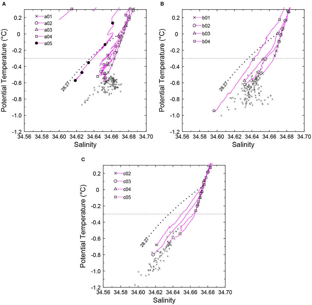
Figure 11. Comparison of θ-S diagrams for moorings and CTD measurement. The gray crosses in (A,B) indicate data for the deepest CT sensors at moorings M1 and M3 in periods P3 and P4, respectively. The gray crosses in (C) indicate data for the deepest CT sensors at moorings M4 in period P4. Magenta lines with symbols indicate θ-S curves for CTD stations (A) a01–a05, (B) b01–b04, and (C) c02–c05. Symbols are plotted at 200 m intervals, starting from the bottom for CTD measurement. The dotted horizontal line indicates θ = −0.3°C.

Figures 11A,B show θ-S diagrams for CTD stations on transects A and B, respectively. Moorings M1 (and M2) and M3 were located on transects A and B, respectively. At stations on these transects, potential temperature was lower than −0.3°C near the bottom, corresponding to newly formed CDBW. Because the number of symbols in the region below θ = −0.3°C was large in Figures 11A,B compared with that in Figure 11C, the thickness of CDBW on transects A and B was larger than that on transect C. As shown in Supplementary Figures 1A–D, cold and less saline water, which is colder than −0.3°C, was present within 200–500 m from the bottom on transects A and B, except for CTD station b07. Thus, supplied from the Cape Darnley polynya, the thickness of the newly formed CDBW significantly increased between transects B and C. A small amount of CDBW was also present at CTD station c05 on transect C. Because SW with salinity higher than 34.6 is distributed in Prydz Bay, which is east of Cape Darnley (Figure 1), cold AABW distributed at CTD station c05 may not be CDBW but newly formed AABW from Prydz Bay (Williams et al., 2016).

Cape Darnley Bottom Water on transect A was warm and saline compared with that on transect B. The gray crosses in Figures 11A,B indicate potential temperature and salinity in periods P3–P4 obtained by the deepest CT sensors at moorings M1 and M3, respectively. Potential temperature and salinity near the bottom obtained at CTD stations roughly coincide with those observed by moorings. Thus, CDBW on transects A and B were the remnant of warm and saline CDBW and cold and less saline CDBW observed at moorings M1 and M3, respectively. As shown in Figures 6, 10, CDBW was present at mooring sites when CTD observation was performed in January 2009. CDBW was present even at CTD stations a01 and b01, which were the offshore most stations on transects A and B, respectively. Thus, CDBW extended offshore, at least beyond these stations. The gray crosses in Figure 11C indicate potential and salinity in period P4 obtained by the deepest CT sensors at moorings M4. Again, potential temperature and salinity obtained at CTD stations on transect C roughly coincide with those observed by mooring M4. Although CDBW observed at mooring M4 was colder than that at mooring M3, potential temperature and salinity at moorings M3 and M4 were approximately aligned on the same line. Thus, the source waters of CDBW observed at these moorings have characteristics similar to each other. Although newly formed AABW at mooring M4 may originate from Prydz Bay, CDBW may also reach mooring M4.

3.4. Short-Term Variability of CDBW

As shown in Figure 5, the temporal variability of velocity was amplified when newly formed CDBW reached mooring sites, suggesting that the variability was induced by the outflow of CDBW. Figure 12 shows the variance-preserving spectra of the kinetic energy calculated from the deepest current meter data at moorings M1–M4. For comparison, power spectra calculated from filtered and unfiltered velocities are shown by the solid and dashed lines, respectively. The power spectra had maximum peaks at frequencies of 0.11, 0.27, and 0.23 cpd, which correspond to periods of 9.1, 3.8, and 4.3 days, at moorings M1, M3, and M4, respectively. A second peak was also found at the frequency of 0.20 cpd at mooring M3. No clear peak was found at mooring M2, although the power spectrum was large between the frequencies of 0.02 and 0.03 cpd. The power spectrum also had small peaks associated with O1, K1, M2, and S2 tidal constituents (the dashed line in Figure 12); however, the energy of tidal currents was small.

FIGURE 12

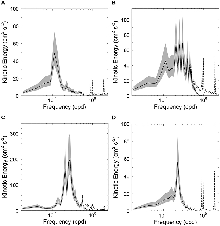
Figure 12. The variance-preserving spectrum of the kinetic energy obtained by the deepest current meter (CM) at moorings (A) M1, (B) M2, (C) M3, and (D) M4. The solid and dashed lines indicate the power spectrum calculated from the filtered and unfiltered velocities, respectively. The 95% confidence limit of the former is shaded. Note that the vertical scale is different in each panel.

The power spectra at other depths also had peaks at the same frequencies as those shown in Figure 12 (not shown). To examine the vertical structure of the variability represented by these peaks, we calculated cross-spectra between the velocity and potential temperature at all depths for each mooring. We used the velocity parallel to the major axes of standard deviation ellipses, u_maj, because it represents the most significant component of the velocity variability. We used u_maj obtained at the deepest depth at each mooring as a reference, and calculated cross-spectra between the velocity and potential temperature at all depths with this reference. Because the velocity data near the bottom were not available at mooring M4, we used potential temperature measured at the deepest depth as a reference for this mooring.

Figure 13 shows the vertical distribution of the phase of the u_maj and potential temperature at the frequency band around the peaks of the power spectra. The phases of u_maj and potential temperature were tilted in the vertical direction, except for u_maj at moorings M3 and M4. The tilt of the phase of u_maj was opposite to that of the potential temperature. The directions of the tilts are consistent with those obtained in a baroclinic instability problem (Pedlosky, 1987). The phase of the potential temperature relative to u_maj at mooring M2 differed from that at moorings M1 and M3 by nearly 180°. This feature is not surprising, because the along-isobath velocity, which is approximately the same as u_maj, has the opposite sign on the onshore and offshore sides of eddies produced by baroclinic instability. The phase difference between potential temperature and u_maj indicates that moorings M1 and M3 were located on the offshore side of eddies, whereas mooring M2 was located on the onshore side of eddies (Pedlosky, 1987).

FIGURE 13

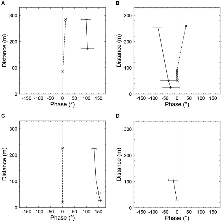
Figure 13. Vertical distribution of the phase of potential temperature (solid line and pluses) and u_maj (dashed line and crosses) at moorings (A) M1, (B) M2, (C) M3, and (D) M4. The phase in the frequency band of 0.094–0.156, 0.25–0.313, 0.25–0.313, and 0.156–0.234 cpd is shown for moorings M1, M2, M3, and M4, respectively. The vertical axis indicates the height from the bottom. The horizontal bars indicate the 95% confidence limit of the phase. The symbols are not drawn at depths where the 95% confidence limit exceeds 60°.

We compare the frequency of the variability obtained at moorings with that of a baroclinically unstable wave theoretically predicted by a three-layer quasi-geostrophic model (refer to Appendix for details). For simplicity, we adopted a quasi-geostrophic model, although the quasi-geostrophic approximation may not be exactly valid at mooring sites. The interface between the first and second layers represents the main pycnocline, and the third layer represents the newly formed CDBW. Using this model, we calculated the complex phase velocity, c, of the unstable wave. The angular frequency and growth rate of the unstable wave are expressed as kc_r and kc_i, respectively, where k is the wavenumber and c_r and c_i are the real and imaginary parts of c, respectively.

Since the peak of the power spectrum was clear and the phase of potential temperature was significantly tilted at mooring M3, we focus on this mooring. Based on the results of the mooring measurements, we set the thickness of the third layer, H₃ = 200 m, the basic flow in the third layer, U₃ = −0.2 ms⁻¹, and the density difference between the second and third layers, Δρ₂ = 0.03 kg m⁻³. We determined the thickness of the first layer, H₁, and the density difference between the first and second layers, Δρ₁, based on the depth of the node and the internal deformation radius of the first baroclinic mode, respectively, calculated from the results of the CTD measurement. For simplicity, we assumed that the basic flow in the first and second layers vanishes and that the perturbation is uniform in the direction normal to the basic flow. To determine the bottom slope, α, we fitted the bottom depth around mooring M3 with a linear function, using a Gaussian weight. The bottom slope was 0.05 and 0.04, when the e-folding scale of the Gaussian weight was 1 and 2 km, respectively. We neglected the meridional change of the planetary vorticity because it is small compared with the change in the potential vorticity due to the bottom slope.

Figure 14 shows the growth rate, kc_i, and the angular frequency, kc_r, of the most unstable wave as a function of the bottom slope, α. The basic flow was unstable when α was <0.09. The dotted horizontal line indicates the angular frequency of the peak of the power spectrum at mooring M3. Because the bottom slope at mooring M3 was 0.04–0.05, the frequency of the variability at mooring M3 agrees with that of the most unstable wave. To examine the sensitivity of kc_r on the speed of basic flow, U₃, we changed U₃ by ±30% (gray lines in Figure 14). We find that kc_r does not significantly depend on the value of U₃. We also verified that kc_r does not significantly depend on H₃, Δρ₂, and other parameters. Thus, the variability observed at mooring M3 is most likely induced by the instability of CDBW flowing along the bottom.

FIGURE 14

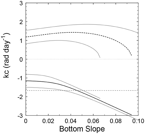
Figure 14. The angular frequency, kc_r, (solid line) and the growth rate, kc_i, (dashed line) of the most unstable wave as a function of the bottom slope, α. The dotted horizontal line indicates the angular frequency of the peak of the power spectrum at mooring M3. The gray lines indicate kc_r and kc_i obtained when U₃ was changed by ±30%. The gray line for kc_r is not drawn when the unstable wave is absent.

4. Summary

We examined the seasonal evolution of CDBW, using results of moorings and CTD measurement in the slope region off the Cape Darnley polynya. Starting in April, the potential temperature and salinity decreased and γ_n increased, indicating that newly formed CDBW arrived at the mooring sites. CDBW first arrived at mooring M2, which was located in the western and shallow region. Then, CDBW subsequently spread to the mooring sites in the more offshore and eastern regions by September. Along with the arrival of CDBW, the current speed near the bottom increased at moorings M2 and M3, suggesting the flow was induced by CDBW. The newly formed CDBW was distributed within 100–300 m or more from the bottom.

θ-S properties of CDBW varied seasonally. From a θ-S diagram for moored CT sensors, it is suggested that CDBW is formed by the mixing between two water masses: one is cold and less saline water corresponding to the source water of CDBW and the other is warm and saline ambient water. The seasonal variation of θ-S properties of CDBW indicated that the salinity of the source water of CDBW increased with time. Based on the distribution of water properties on a θ-S diagram, we estimated the salinity, S_SW, of the source water of CDBW. The value of S_SW roughly agrees with the salinity of SW observed near the shelf break. S_SW at mooring M2, which was located in the upper part of the slope, started to increase in late April, which is about 2 months after the onset of sea-ice production. Then, S_SW at other mooring sites started to increase from May to September. As long as sea ice was produced, both S_SW and salinity at the shelf break continued to increase. These results indicate that S_SW increased with time because brine rejected in the Cape Darnley polynya accumulated on the shelf. Thus, S_SW and θ-S properties of CDBW vary due to the accumulation of brine in the Cape Darnley polynya.

Two types of CDBW were identified. Cold and less saline CDBW was present at mooring M3, which was located in Wild Canyon, and warm and saline CDBW was present at moorings M1 and M2, which were located in and upstream of Daly Canyon, respectively. Hence, CDBW in Daly Canyon was warmer and saltier than that in Wild Canyon. S_SW of the source water of CDBW in Daly Canyon was also higher than that in Wild Canyon. Because Daly Canyon is located to the west of Wild Canyon, these results suggest that brine rejected in the Cape Darnley polynya accumulated in SW as it is advected westward. Thus, the sea-ice production in the Cape Darnley polynya is an important factor that affects the variation of θ-S properties of CDBW in both space and time. According to CTD measurement, the thickness of newly formed AABW significantly increased between the transects located on the eastern and western sides of the Cape Darnley polynya, corresponding to the supply of CDBW from the polynya. Both the cold and less saline CDBW and warm and saline CDBW spread offshore along Wild and Daly Canyons, respectively.

When CDBW arrived at the mooring sites, the short-term variability of the velocity was apparent, especially at mooring M3. The power spectrum of the kinetic energy had peaks at periods between 3.8 and 9.1 days. The vertical distribution of the phase of u_maj and the potential temperature was mostly tilted in the opposite direction, being consistent with that obtained in a baroclinic instability problem. The frequency of the variability at mooring M3 agrees with that of the most unstable wave obtained by a three-layer quasi-geostrophic model. Thus, the variability was most likely induced by the baroclinic instability of CDBW.

In this study, we focused on the mixing process of CDBW in the slope region. While S_SW roughly agreed with the salinity of SW near the shelf break, more saline SW with a salinity exceeding S_SW was also observed. SW probably mixes with less saline mCDW near the shelf break, as suggested by Foster and Carmack (1976). To understand the entire formation process of CDBW, we need winter hydrographic data covering broader regions. Hydrographic observations from floats and instrumented seals may be able to contribute to the increase of such data (Wong and Riser, 2013; Williams et al., 2016). These analyses are left for future research.

Data Availability Statement

The datasets presented in this article are not readily available because analysis by authors have not fully finished for some data. Requests to access the datasets should be directed to Kay I. Ohshima, b2hzaGltYSYjeDAwMDQwO2xvd3RlbS5ob2t1ZGFpLmFjLmpw.

Author Contributions

GM analyzed all the data and wrote the manuscript with comments by all other authors. YF conducted the mooring observations with KO, YM, and DS. YK and DH conducted hydrographic observations. MF processed the bathymetric data. YN contributed to bathymetry data acquisition. The project was led by KO. All authors contributed to the article and approved the submitted version.

Funding

The present study was supported by Grants-in-Aid for Scientific Research (20221001, 20540419, 25241001, 17H01157, 17H06317, 20H05707, and 23340135) of the Ministry of Education, Culture, Sports, Science and Technology in Japan, and the Science Program of Japanese Antarctic Research Expedition.

Conflict of Interest

The authors declare that the research was conducted in the absence of any commercial or financial relationships that could be construed as a potential conflict of interest.

Publisher's Note

All claims expressed in this article are solely those of the authors and do not necessarily represent those of their affiliated organizations, or those of the publisher, the editors and the reviewers. Any product that may be evaluated in this article, or claim that may be made by its manufacturer, is not guaranteed or endorsed by the publisher.

Acknowledgments

We are deeply indebted to the officers, crew, and scientists on board TR/V Umitaka-maru, R/V Hakuho-maru, and icebreaker Shirase for their help with field observations. The sea ice production data were provided by Kazuki Nakata.

Supplementary Material

The Supplementary Material for this article can be found online at: https://www.frontiersin.org/articles/10.3389/fmars.2021.657119/full#supplementary-material

References

Amante, C., and Eakins, B. W. (2009). ETOPO1 Global Relief Model converted to PanMap layer format. NOAA-National Geophysical Data Center. PANGAEA. doi: 10.1594/PANGAEA.769615

CrossRef Full Text

Aoki, S., Katsumata, K., Hamaguchi, M., Noda, A., Kitade, Y., Shimada, K., et al. (2020). Freshening of antarctic bottom wate off cape darnley, East Antarctica. J. Geophys. Res. 125:e2020JC016374. doi: 10.1029/2020JC016374

CrossRef Full Text | Google Scholar

Arndt, J. E., Schenke, H. W., Jakobsson, M., Nitsche, F. O., Buys, G., Goleby, B., et al. (2013). The International Bathymetric Chart of the Southern Ocean (IBCSO) version 1.0—a new bathymetric compilation covering circum-Antarctic waters. Geophys. Res. Lett. 40, 3111–3117. doi: 10.1002/grl.50413

CrossRef Full Text | Google Scholar

Baines, P. G., and Condie, S. (1998). “Observations and modelling of Antarctic downslope flows: a review,” in Ocean, Ice, and Atmosphere: Interactions at the Antarctic Continental Margin, Vol. 75 of Antarctic Research Series, eds S. Jacobs and R. Weiss (Washington, DC: AGU), 29–49.

Google Scholar

Chapman, D. C., and Gawarkiewicz, G. (1995). A numerical study of dense water formation and transport on a shallow, sloping continental-shelf. J. Geophys. Res. 100, 4489–4507. doi: 10.1029/94JC01742

CrossRef Full Text | Google Scholar

Couldrey, M. P., Jullion, L., Naveira Garabato, A. C., Rye, C., Herraiz-Borreguero, L., Brown, P. J., et al. (2013). Remotely induced warming of Antarctic bottom water in the eastern Weddell gyre. Geophys. Res. Lett. 40, 2755–2760. doi: 10.1002/grl.50526

CrossRef Full Text | Google Scholar

Emery, W., and Thomson, R. (2001). Data Analysis Methods in Physical Oceanography. Boston, MA: Elsevier Science.

Google Scholar

Foster, T. D., and Carmack, E. C. (1976). Frontal zone mixing and Antarctic bottom water formation in southern Weddell Sea. Deep Sea Res. 23, 301–317. doi: 10.1016/0011-7471(76)90872-X

CrossRef Full Text | Google Scholar

Hirano, D., Kitade, Y., Ohshima, K. I., and Fukamachi, Y. (2015). The role of turbulent mixing in the modified shelf water overflows that produce cape darnley bottom water. J. Geophys. Res. 120, 910–922. doi: 10.1002/2014JC010059

CrossRef Full Text | Google Scholar

Jackett, D. R., and McDougall, T. J. (1997). A neutral density variable for the world's oceans. J. Phys. Oceanogr. 27, 237–263. doi: 10.1175/1520-0485(1997)027andlt;0237:ANDVFTandgt;2.0.CO;2

CrossRef Full Text | Google Scholar

Jacobs, S. S., Amos, A. F., and Bruchhau, P. M. (1970). Ross-Sea oceanography and Antarctic bottom water formation. Deep Sea Res. 17, 935. doi: 10.1016/0011-7471(70)90046-X

CrossRef Full Text | Google Scholar

Kitade, Y., Shimada, K., Tamura, T., Williams, G. D., Aoki, S., Fukamachi, Y., et al. (2014). Antarctic bottom water production from the vincennes bay polynya, East Antarctica. Geophys. Res. Lett. 41, 3528–3534. doi: 10.1002/2014GL059971

CrossRef Full Text | Google Scholar

Mantyla, A. W., and Reid, J. L. (1983). Abyssal characteristics of the world ocean waters. Deep Sea Res. A Oceanogr. Res. Pap. 30, 805–833. doi: 10.1016/0198-0149(83)90002-X

CrossRef Full Text | Google Scholar

Meijers, A. J. S., Klocker, A., Bindoff, N. L., Williams, G. D., and Marsland, S. J. (2010). The circulation and water masses of the Antarctic shelf and continental slope between 30 and 80°E. Deep Sea Res. II Top. Stud. Oceanogr. 57, 723–737. doi: 10.1016/j.dsr2.2009.04.019

CrossRef Full Text | Google Scholar

Meredith, M., Locarnini, R., Van Scoy, K., Watson, A., Heywood, K., and King, B. (2000). On the sources of weddell gyre antarctic bottom water. J. Geophys. Res. 105, 1093–1104. doi: 10.1029/1999JC900263

CrossRef Full Text | Google Scholar

Morrison, A. K., Hogg, A. M., England, M. H., and Spence, P. (2020). Warm Circumpolar Deep Water transport toward Antarctica driven by local dense water export in canyons. Sci. Adv. 6:eaav2516. doi: 10.1126/sciadv.aav2516

PubMed Abstract | CrossRef Full Text | Google Scholar

Nakata, K., Ohshima, K. I., and Nihashi, S. (2019). Estimation of thin-ice thickness and discrimination of ice type from AMSR-E passive microwave data. IEEE Trans. Geosci. Remote Sens. 57, 263–276. doi: 10.1109/TGRS.2018.2853590

CrossRef Full Text | Google Scholar

Nakata, K., Ohshima, K. I., and Nihashi, S. (2021). Mapping of active frazil for Antarctic coastal polynyas, with an estimation of sea-ice production. Geophys. Res. Lett. 48:e2020GL091353. doi: 10.1029/2020GL091353

CrossRef Full Text | Google Scholar

Nakayama, Y., Ohshima, K. I., Matsumura, Y., Fukamachi, Y., and Hasumi, H. (2014). A numerical investigation of formation and variability of Antarctic bottom water off cape darnley, East Antarctica. J. Phys. Oceanogr. 44, 2921–2937. doi: 10.1175/JPO-D-14-0069.1

CrossRef Full Text | Google Scholar

Nihashi, S., and Ohshima, K. I. (2015). Circumpolar mapping of Antarctic coastal polynyas and landfast sea ice: relationship and variability. J. Climate 28, 3650–3670. doi: 10.1175/JCLI-D-14-00369.1

CrossRef Full Text | Google Scholar

Ohshima, K. I., Fukamachi, Y., Williams, G. D., Nihashi, S., Roquet, F., Kitade, Y., et al. (2013). Antarctic Bottom Water production by intense sea-ice formation in the Cape Darnley polynya. Nat. Geosci. 6, 235–240. doi: 10.1038/ngeo1738

CrossRef Full Text | Google Scholar

Orsi, A. H., Johnson, G. C., and Bullister, J. L. (1999). Circulation, mixing, and production of Antarctic Bottom Water. Progr. Oceanogr. 43, 55–109. doi: 10.1016/S0079-6611(99)00004-X

CrossRef Full Text | Google Scholar

Orsi, A. H., and Wiederwohl, C. L. (2009). A recount of Ross Sea waters. Deep Sea Res. II Top. Stud. Oceanogr. 56, 778–795. doi: 10.1016/j.dsr2.2008.10.033

CrossRef Full Text | Google Scholar

Pedlosky, J. (1987). Geophysical Fluid Dynamics. New York, NY: Springer-Verlag.

Google Scholar

Rintoul, S. R. (1998). “On the origin and influence of Adélie Land Bottom Water,” in Ocean, Ice, and Atmosphere: Interactions at the Antarctic Continental Margin, Vol. 75 of Antarctic Research Series, eds S. Jacobs and R. Weiss (Washington, DC: AGU), 151–171.

Tamura, T., Ohshima, K. I., and Nihashi, S. (2008). Mapping of sea ice production for Antarctic coastal polynyas. Geophys. Res. Lett. 35:L07606. doi: 10.1029/2007GL032903

CrossRef Full Text | Google Scholar

Whitworth, T. III., and Orsi, A. H. (2006). Antarctic Bottom Water production and export by tides in the Ross Sea. Geophys. Res. Lett. 33:L12609. doi: 10.1029/2006GL026357

CrossRef Full Text | Google Scholar

Whitworth, T. III., Orsi, A. H., Kim, S. J., Nowlin, W. D., and Locarnini, R. (1998). “Water masses and mixing near the Antarctic slope front,” in Ocean, Ice, and Atmosphere: Interactions at the Antarctic Continental Margin, Vol. 75 of Antarctic Research Series, eds S. Jacobs and R. Weiss (Washington, DC: AGU), 1–27.

Google Scholar

Williams, G. D., Aoki, S., Jacobs, S. S., Rintoul, S. R., Tamura, T., and Bindoff, N. L. (2010). Antarctic Bottom Water from the Adélie and George V Land coast, East Antarctica (140-149°E). J. Geophys. Res. 115:C04027. doi: 10.1029/2009JC005812

CrossRef Full Text | Google Scholar

Williams, G. D., Bindoff, N. L., Marsland, S. J., and Rintoul, S. R. (2008). Formation and export of dense shelf water from the Adélie Depression, East Antarctica. J. Geophys. Res. 113:C04039. doi: 10.1029/2007JC004346

CrossRef Full Text | Google Scholar

Williams, G. D., Herraiz-Borreguero, L., Roquet, F., Tamura, T., Ohshima, K. I., Fukamachi, Y., et al. (2016). The suppression of Antarctic Bottom Water formation by melting ice shelves in Prydz Bay. Nat. Commun. 7:12577. doi: 10.1038/ncomms12577

PubMed Abstract | CrossRef Full Text

Wong, A. P. S., and Riser, S. C. (2013). Modified shelf water on the continental slope north of Mac Robertson Land, East Antarctica. Geophys. Res. Lett. 40, 6186–6190. doi: 10.1002/2013GL058125

CrossRef Full Text | Google Scholar