Machine Learning Incorporated With Causal Analysis for Short-Term Prediction of Sea Ice

Accurate and fast prediction of sea ice conditions is the foundation of safety guarantee for Arctic navigation. Aiming at the imperious demand of short-term prediction for sea ice, we develop a new data-driven prediction technique for the sea ice concentration (SIC) combined with causal analysis. Through the causal analysis based on kernel Granger causality (KGC) test, key environmental factors affecting SIC are selected. Then multiple popular machine learning (ML) algorithms, namely self-adaptive differential extreme learning machine (SaD-ELM), classification and regression tree (CART), random forest (RF) and support vector regression (SVR), are employed to predict daily SIC, respectively. The experimental results in the Barents-Kara (B-K) sea show: (1) compared with correlation analysis, the input variables of ML models screened out by causal analysis achieve better prediction; (2) when lead time is short (<3 d), the four ML algorithms are all suitable for short-term prediction of daily SIC, while RF and SaD-ELM have better prediction performance with long lead time (>3 d); (3) RF has the best prediction accuracy and generalization ability but hugely time consuming, while SaD-ELM achieves more favorable performance when taking computational complexity into consideration. In summary, ML is applicable to short-term prediction of daily SIC, which develops a new way of sea ice prediction and provides technical support for Arctic navigation.

Introduction

There have been unprecedented decreases in the amount of Arctic sea ice due to global warming. The Arctic Ocean is rapidly transforming into a navigable ocean, making the exploitation and utilization of marine resources viable in this region. Sea ice conditions, mainly including sea ice concentration (SIC) and sea ice thickness (SIT), not only induce additional resistance, thereby increasing sailing fuel consumption but also may cause damage to the ship hull and propeller. Therefore, sea ice makes Arctic routes fraught with risks and unexpected costs. For the present, sea ice observation and empirical prediction are widely conducted to reduce the risk caused by sea ice in the Arctic navigation (Li et al., 2019). However, the role of these approaches is minimal due to complex variations of sea ice. There is room to further improve prediction with more advanced techniques, aiming at accurate and fast sea ice prediction for supporting Arctic navigation.

At present, many studies have been devoted to sea ice prediction, developing a number of forecasting approaches. All of those are classified into two kinds: numerical models and statistical models. Numerical prediction is based on sea ice numerical models, including dynamic models, thermodynamic models and dynamic-thermal coupling models. Many numerical models show some predictive skill at seasonal to interannual time scales. Chevallier et al. (2015) described the initialization techniques and the forecast protocol of the Global Climate Model (GCM), and developed the seasonal forecast of the pan-Arctic sea ice extent using the GCM-based seasonal prediction system. Mitchell et al. (2017) investigated the regional forecast skill of the Arctic sea ice in a Geophysical Fluid Dynamics Laboratory (GFDL) seasonal prediction system, using a coupled atmosphere-ocean-sea ice-land model. Gascard et al. (2017) discussed the ability to hindcast and predict sea ice conditions in the Arctic Ocean. In his research, the CMIP5 (Coupled Model Inter-comparison Project Phase 5) was used to provide ranges of potential future sea ice conditions on large scales. Jun (2020) have presented characteristics of the predictabilities of weather, sea ice and ocean waves under extreme atmospheric conditions over the Arctic Ocean in supporting Arctic navigation. In terms of dynamic and thermodynamic processes of sea ice, the numerical prediction is relatively accurate but has high time complexity, which poses the greatest challenge for short-term and fast sea ice prediction during navigation safeguarding, especially for sailing adjustment according to sea ice changes.

Meanwhile, there has been some development of statistical forecast for the Arctic sea ice, no matter the forecast focused on the basin as a whole or for specific regions. In statistical models, statistical relationships between sea ice and proceeding environmental factors are built by time series analysis, and sea ice is predicted according to variations of environmental factors. Models about sea ice statistical prediction are relatively simple, mainly including one-dimensional linear regression or multivariate linear regression (Drobot and Maslanik, 2002; Chen and Yuan, 2004). Given its cost effectiveness, scholars are motivated to develop more advanced statistical models: Drobot et al. (2006) developed a statistical model to predict the pan-Arctic minimum ice extent based on multiple linear regression and used the satellite-observed ice concentration, surface skin temperature, albedo and downwelling longwave radiative flux as predictor variables. Lindsay et al. (2008) explored the forecasting ability of a linear empirical model for sea ice extent, using as predictors historical information about the ocean and ice obtained from an ice-ocean model retrospective analysis. Yuan et al. (2016) built a linear Markov model for monthly SIC forecasting at pan-Arctic grid points for all seasons. He also assessed the sea ice predictability at different spatial locations over all seasons. Wang et al. (2016) adopted the vector autoregressive (VAR) model for predicting the summertime (May to September) Arctic SIC at the intra-seasonal time scale, using only the daily sea ice data and without direct information of the atmosphere and ocean. To deal with the nonlinearity in sea ice prediction, Zhang et al. (2017) established a SIT prediction model based on BP neural network trained by a large number of observed data. However, sea ice prediction is a very challenging task under the changing Arctic climate system (Stroeve et al., 2008, 2014). Sea ice is a coupled nonlinear system influenced by varieties of meteorological and oceanic factors, causing drastic diurnal variations and poor continuity of time series. Unfortunately, most statistical models with linear assumption fail to describe complex nonlinear relationships.

All in all, numerical prediction and statistical prediction of sea ice achieve varying degrees of success but still have some shortcomings: (1) It is necessary for sea ice numerical models based on dynamic and thermodynamic equations to input strict initial conditions, causing high computational complexity (Lindsay et al., 2008; Wang et al., 2016; Yuan et al., 2016), which cannot meet the requirements of fast and real-time prediction in supporting Arctic navigation. (2) Statistical models run fast and are easy to understand but have limited ability to capture non-linearity and non-stationarity of sea ice time series because of their linear and stationary assumptions (Stroeve et al., 2014; Gascard et al., 2017). (3) Both numerical and statistical models mainly focus on the monthly and quarterly forecast of sea ice, while short-term and daily prediction is rarely studied. Monthly prediction of sea ice makes little sense to ship navigation. It is urgent to develop new daily sea ice forecasting models for fast and accurate prediction.

In recent years, with the development of artificial intelligence, machine learning (ML), more advanced data-driven technique, is capturing people’s attention, including neural network, decision tree (DT), naïve Bayes and support vector machine, etc. At present, deep neural networks have been demonstrated to predict the Arctic sea ice: Chi and Kim (2017) proposed a deep-learning-based model using the long- and short-term memory network (LSTM) in comparison with a traditional statistical model. Their model showed good performance in the 1-month prediction of SIC. Kim et al. (2019) put forward a near-future SIC prediction model (10–20 years) with deep learning networks and the Bayesian model averaging ensemble, lowing forecasting errors effectively. Wang et al. (2017) applied the convolutional neural network (CNN) to estimate SIC in the Gulf of Saint Lawrence from synthetic-aperture-radar (SAR) imagery, showing the superiority of CNN model in SIC estimation. Compared with numerical models and classic statistical models, ML algorithms simplify the tedious and intricate calculations, and they are good at expressing non-linear relationships of variables (Li and Liu, 2020). However, the previous studies using ML techniques still focused on the long-term prediction of SIC. The short-term prediction at a finer time scale is more important for navigation and maritime industries (Schweiger and Zhang, 2015). In addition, other ML algorithms have not been applied to sea ice prediction except neural networks. Therefore, we will try adopting various ML algorithms for short-term sea ice prediction and compare their model performance to discuss the applicability and reliability of ML in sea ice prediction.

Additionally, predictor selection plays a vital role in prediction, known as “Feature Selection” in modeling with ML (Poggio et al., 2000). Effective predictors selection can greatly reduce the running time, improve the prediction accuracy as well as increase the interpretability of the prediction model. In classical statistical forecasting models, selection methods for predictors mainly include stepwise regression, time-lag correlation analysis and teleconnection analysis, etc. However, there has been a strong argument against using correlation analysis for this purpose in the causal analysis community. Liang (2014) made clear that two variables with a strong correlation did not necessarily have a strong causality. It is worth noting that causal analysis becomes a more advanced way of detecting relationships. Bai et al. (2017) and Li and Liu (2018) applied causal analysis to predictor selection and significantly improved the forecasting accuracy. It is well-known that daily and monthly sea ice change are affected by all kinds of factors in different atmospheric processes (Fang and Wallace, 1994; Kang et al., 2014; Cvijanovic and Caldeira, 2015; Gong and Luo, 2017). In our research, we will apply causal analysis, rather than correlation analysis, to select predictors and further discuss the influence of different factors on the prediction accuracy of sea ice.

The Arctic is rapidly transforming into a navigable ocean due to global warming. In this case, the development of new prediction techniques of sea ice has become a high priority. Regional sea-ice predictions at finer time scales are a pressing need for Arctic navigation. In this article, we will combine causal analysis and various popular ML algorithms for SIC prediction to discuss the applicability and reliability of ML in sea ice short-term prediction by error analysis, exploring new prediction ways. The rest of the paper is organized as follows: section “Theory and Method” explains the theoretical formulations and proposes a detailed elaboration of our prediction model. Application and results analysis are showed in section “Short-Term Prediction of Daily SIC.” section “Conclusion” concludes the presented studies.

Theory and Method

This section makes a specific introduction of various ML algorithms and the causal analysis technique—Granger causality test. Then the ML-based prediction technique with causal analysis will be proposed.

ML Algorithm

We select popular ML algorithms, including extreme learning machine (ELM), DT, random forest (RF) and support vector regression (SVR), for daily SIC prediction. The principle and characteristics of these algorithms are listed below.

(1) Extreme Learning Machine

Extreme learning machine is a novel single hidden layer feedforward neural network, overcoming the weakness of slow convergence and local optimum in conventional neural networks. However, the random setting of initial weights and threshold easily results in weak stability and poor generalization. To deal with this deficiency, Cao et al. (2012) used the self-adaptive differential evolution (SaD) algorithm to improve ELM and further proposed the self-adaptive differential extreme learning machine (SaD-ELM), which is used in our research.

(2) Decision Tree

Decision tree is constructed recursively by dividing nodes according to the square error minimization criterion, and the mean value of all leaf nodes is taken as the predicted result. DT is suitable for dealing with interactions among features (or predictors), easy to interpret, and runs fast. In this article, we will choose one kind of DT, classification and regression tree (CART), to construct the prediction model.

(3) Random Forest

Based on the idea of ensemble learning, DT is used as the base learning machine to establish an ensemble model, namely RF. The predicted value of RF is obtained by taking the mean prediction of all DTs. Balancing the error of data sets gives RF the advantage of not easy to overfit; besides that, it also has great robustness.

(4) Support Vector Regression

Support vector regression adheres to the principle of structural risk minimization seeking to minimize an upper bound of generalization error and has good generalization ability. It can deal with nonlinear interactions of features and solve the problem of high-dimensional input space.

Causal Analysis

Input variable selection is of vital importance in ML. Irrelevant variables, used as inputs of a regression machine, can unnecessarily increase the time consuming of a prediction system, as well as degrade the generalization ability and interpretability (Li and Liu, 2020). In previous studies about time series prediction with ML algorithms, methods based on correlation coefficient and univariate regression are still the most common data-based tools to select predictors by analyzing associations (Li and Liu, 2019). Such approaches are useful in daily practice but provide few insights into the causal mechanisms that underlie the dynamics of a system, which is important in meteorology and oceanography. Causal inference methods can overcome some of the key shortcomings of such correlation analysis (Runge et al., 2019).

Nowadays, the relationships mining from time series by causal analysis in the earth system is a frontier issue. Some hidden relationships in the earth system have been detected by causal analysis, which cannot be identified by correlation analysis. For example, Sugihara et al. (2012) showed an example from ecology demonstrating that traditional regression analysis was unable to identify the complex nonlinear interactions among sardines, anchovy, and sea surface temperature (SST) in the California Current ecosystem. A nonlinear causal state-space reconstruction method reveals that SST is a common driver of both sardine and anchovy abundances. Marlene et al. (2016) detected that Barents-Kara SIC is an important driver of mid-latitude circulation, influencing winter Arctic Oscillation (AO), by causal inference method. McGraw and Barnes (2020) also used the Granger causality method to examine the causal relationship between Arctic sea ice and atmospheric circulations. These studies prove that causal analysis has a stronger ability to mine relationships than correlation analysis, which is beneficial to changes explanation. It is a promising approach to select predictors in the prediction system.

Granger causality test (GC) is a classic causal detection method proposed by Granger (1969) and Sims (1972). The basic definition is: when the historical information of variables X and Y are included, the prediction accuracy of Y is better than that of the historical information of Y alone, that is, the introduction of X is conductive to the prediction of Y. In other words, X helps to explain the future change of Y, then X is considered as the Granger cause of Y. This definition is based on the regression and its mathematics expression is shown below.

Regression equation of X and Y is built:

$$Y_t={\displaystyle \sum _{i=1}^k}{\mathrm{\alpha }}_i{Y}_{t-i}+{\displaystyle \sum _{i=1}^k}{\mathrm{\beta }}_i{X}_{t-i}+e_t(1)$$

$$Y_t={\displaystyle \sum _{i=1}^k}{\mathrm{\alpha }}_i{Y}_{t-i}+e_t(2)$$

where: e_t denotes regression error; k is maximum lag order; α_i and β_i denotes regression coefficient. GC is usually assessed according to the statistical test (Krakovská et al., 2018).

Original hypothesis: X is not the Granger cause of Y.

Test statistic:

$$F={\displaystyle \frac{(SS{E}_r-SS{E}_m)/k}{SS{E}_m/(N-2k)}}\sim F(k,N-2k)(3)$$

where: SSE_r is the residual sum of squares of autoregression with Y; SSE_m is the residual sum of squares of regression with X and Y. If FF_a, then X is the Granger cause of Y.

However, classic GC is only suitable for stationary time series and has low detection power for high-dimensional space. An attempt to extend GC to nonlinear cases by using the theory of reproducing kernel Hilbert spaces was proposed by Marinazzo et al. (2008), namely KGC test. The method investigates Granger causality in the feature space of suitable kernel functions. Instead of assessing the presence of causality by means of a single statistical test, KGC constructs a causality index to express the strength of causal relationships. The role of the two time series can be reversed to evaluate the causality index in the opposite direction. KGC works well for causality detection of nonlinear time series and explains some hidden relations in complex systems (Krakovská et al., 2018). In our research, we will adopt the KGC test to select input factors of SIC prediction by the shared MATLAB toolbox¹, introducing causal analysis to ML.

Prediction Model

This subsection presents a data-driven prediction model based on ML and causal analysis. The main technique scheme and processing stages are illustrated as follow, including factor management, model construction, and model prediction.

Factor Management: First, quality control and normalization processing of data are carried out, and data are divided into training sets and testing sets. Then, based on KGC test, causal analysis of environmental factors is conducted to select the best predictor variables of SIC.

Model Construction: Predictors are taken as input variables and SIC is the response variable. SaD-ELM, CART, RF, and SVR are employed to build prediction models, respectively. The initial parameters are set according to the characteristics of each algorithm, then, based on training sets, the 10-fold cross-validation method is used for parameter tuning and prediction models are trained completely.

Model Prediction: The prediction result is obtained by means of cross-validation. The predictive ability of different models are compared by error analysis, and the applicability of ML algorithms for sea ice prediction is discussed in detail.

Short-Term Prediction of Daily SIC

This section conducts SIC prediction experiments with the proposed technique. The performance levels of different algorithms are compared in order to discuss the applicability and reliability of ML in sea ice prediction.

Study Area and Data Introduction

Barents Sea and Kara Sea (B-K) are important marginal seas of the Arctic Ocean, which is one of the most important routes for the Arctic navigation. Sea ice of the B-K sea decreases dramatically due to climate change, having a remarkable impact on navigation safety. This article predicts SIC at day time scales in the B-K sea (70–80°N, 20–80°E).

Sea ice concentration datasets are obtained from Climate Data Record (CDR) provided by the National Snow and Ice Data Center (NSIDC). SIC is the sea ice–covered area relative to the total at a given location in the ocean, and thus ranges from 0 to 1 (or 0–100%). By incorporating data from multiple sensors, including SSMR, SSM/I, and SSMI/S, SIC datasets are generated with the bootstrap algorithm. The SIC data are available from November 1st, 1978 every day and have the spatial resolution of 25 km × 25 km². In our research, daily time series of SIC from January 1st, 2009 to December 31st, 2018 are used for experiments and resampled to 1° × 1° grids by the linear interpolation method. The temporal-spatial number of SIC grid is [3652 days × (61 × 11) grids].

The daily change of B-K SIC is affected by various factors in complex atmospheric processes (Fang and Wallace, 1994). The solar radiation heats the surface of sea ice, causing a decline of sea ice by raising sea temperature (Screen and Simmonds, 2010). Local wind forces cause sea ice drifts, affecting sea ice motion and destruction (Shimada et al., 2006; Guemas et al., 2016). Cvijanovic and Caldeira (2015) pointed out that the increase in CO₂ is critical for decline of sea ice. Gong and Luo (2017) revealed the presence of Ural blocking with a positive North Atlantic Oscillation is important for the variability of sea ice. They also found the decline of B-K SIC lags the total water by about 4 days. To sum up, environmental factors causing the daily variation of SIC include dynamical variables and thermodynamic variables. According to the fifth assessment report of the Intergovernmental Panel on Climate Change (IPCC), we preliminarily select low cloud cover, sea level pressure, 2 m air temperature, northward heat flux, northward water vapor flux, 2 m wind speed, SST, albedo and total column water vapor as predictor variables, named LCC, SLP, AT, HF, WVF, WD, SST, AL, and WV. Their datasets are obtained from the European Centre for Medium Range Weather Forecast (ECMWF) and have the same temporal-spatial resolution with SIC³.

Predictor variables and SIC have different orders of magnitude. In order to eliminate the impact of different orders of magnitude on causal analysis and prediction and to speed up the training of ML algorithms, all variables need to be normalized according to Eq. 4.

$$X={\displaystyle \frac{x-x_{min}}{x_{max}-x_{min}}}(4)$$

where: X is the normalized value; x is the original value; x_max and x_min denote maximum and minimum of original values.

Causality Detection

kernel Granger causality is capable of mining causal relationships from time series of multiple variables, so we average variables of all grids (61 × 11) in the B-K sea and generate time series of nine predictors and SIC. Each time series comprise 3652 days. The inhomogeneous polynomial function is used in the implementation of KGC test.

Table 1 shows the results of causal analysis between the predictors and SIC. We can see KGC index is asymmetric and directional, so the direction of causality can be identified. The causal analysis shows: SLP and WVF are not the Granger cause of SIC (KGC = 0); the causal relationships between SIC and LCC, HF are weak (KGC fails to pass the significance test). By contrast, there are significant reciprocal causality between SIC and AT, AL; WD, SST, and WV are the unidirectional Granger cause of SIC (WD→SIC, SST→SIC, WV→SIC). Through casual analysis, AT, WD, SST, AL, and WV are the Granger cause of SIC and can significantly explain the future change of SIC.

TABLE 1

Table 1. KGC index between SIC and predictors (statistically significant values at the 95% level are highlighted).

The five predictors selected through causal analysis have theoretical foundations that are related to the physical mechanism of SIC. AT and AL are related to the amount of solar radiation which enables the prediction of SIC to change. The solar radiation heats the surface of ocean as well as sea ice, which causes a rise of SST while also reducing AL on the sea ice by thinning the sea ice (Mahajan et al., 2011). Warm winds from lower latitudes toward the Arctic can melt sea ice (Kang et al., 2014). Changes in SST and SIC have a significant relationship to each other with regards to the heat budget (Rayner et al., 2003; Screen et al., 2013), corresponding to the findings obtained by Granger causality method (McGraw and Barnes, 2020). The re-emergence of sea ice anomalies is also partially interpreted by the persistence of SST anomalies (Guemas et al., 2016). WV is closely related to daily change of SIC and SIC decline lags WV by about 4 days (Gong and Luo, 2017). The previous studies provide a theoretical support for the Granger causality analysis.

As a contrast, we also take correlation analysis between environmental factors and SIC. Pearson correlation coefficient (Table 2) shows that SIC has strong relevance with LCC, AT, HF, WD, SST, AL, and WV. In order to test the validity of causal analysis, we respectively use predictors selected by causal analysis and correlation analysis to build prediction models with ML algorithms, and discuss the impact of different predictors on SIC prediction.

TABLE 2

Table 2. Pearson correlation coefficient between SIC and predictors (statistically significant values at the 95% level are highlighted).

Prediction Experiment Design

To fully discuss the applicability of ML algorithms to short-term sea ice prediction, two experiments are designed: (1) SIC prediction in the Kara Strait (single site: 71°N, 58°E) with different lead times (1, 3, and 5 d). (2) SIC prediction in the B-K sea (region: 70–80°N, 20–80°E) with different lead times (1, 3, and 5 d).

Experiment I: SIC Prediction in the Kara Strait (71°N, 58°E)

To exclude the prediction errors caused by SIC anomalies such as missing value, ice-free value and land, we select SIC greater than 0.1, a total of 1000 samples, for ML modeling. The 10-fold cross-validation approach is adopted to construct prediction models and verify the performance. The samples are divided into ten equal parts. In each prediction experiment, nine groups of samples (training samples) are used to train prediction models, and the remaining one group (testing samples) are used for model validation. root-mean-square error (RMSE), correlation coefficient (R) and mean relative error (MRE), as shown in Eqs 5–7, are employed as evaluation criteria to investigate the performance levels of prediction models quantitatively.

$$\text{RMSE}=\sqrt{{\displaystyle \frac{1}{n}}{\displaystyle \sum _{i=1}^n}{(y-\widehat{y})}^2}(5)$$

$$\text{R}={\displaystyle \frac{\text{Cov}(y,\widehat{y})}{\sqrt{\text{Var}\left(y\right)\cdot \text{Var}\left(\widehat{y}\right)}}}(6)$$

$$\text{MRE}={\displaystyle \frac{1}{n}}{\displaystyle \sum _{i=1}^n}{\displaystyle \frac{\left|y-\widehat{y}\right|}{y}}(7)$$

where: y is the observation; $\widehat{y}$ is the prediction.

Taking predictors selected by causal analysis (AT, WD, SST, AL, and WV) and correlation analysis (LCC, AT, HF, WD, SST, AL, and WV) as input variables, respectively, the four ML algorithms are adopted to build prediction models. It is well known that historical information of SIC helps to explain the future change of SIC (Deser and Teng, 2008). Therefore, past SIC is also taken as the predictor. Figure 1 shows the inputs of prediction model.

FIGURE 1

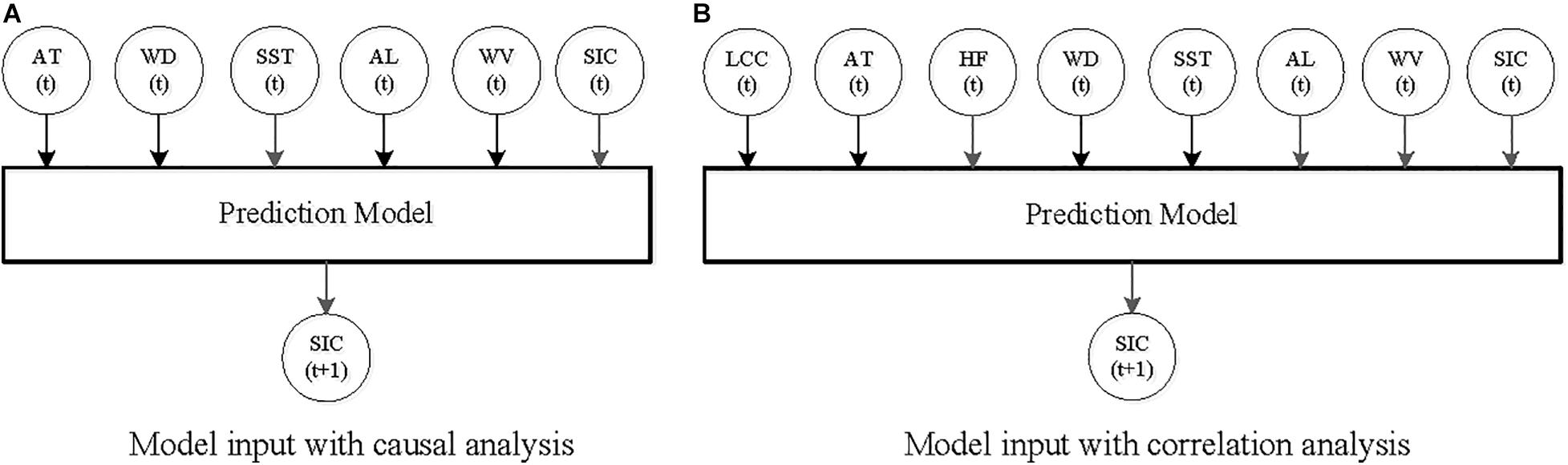
Figure 1. Prediction mechanism of ML model. (A) Model input with causal analysis. (B) Model input with correlation analysis.

In the model training of the four ML algorithms: SaD-ELM has a lot of parameters so we set them by referring to Cao et al. (2012). For SVR, the parameters involve the penalty coefficient and small positive number, in which both parameters are embedded in dual problem formalism. Here, we respectively set penalty coefficient and small positive number at 15 and 0.001, according to Liu et al. (2020).

For CART and RF, parameter calibrations are subjected to sensitivity analysis, which is conducted by “GridSearchCV” function provided by scikit-learn module, which is a function library for ML including all kinds of classification, regression and clustering algorithms. RMSE is used to measure the errors of results. The smaller the RMSE, the more favorable is the performance of the predicted outcome. For CART, the maximum depth of the tree (max_depth) and the number of node samples (num_samples) are chosen by performing sensitivity analysis. Figure 2 plots the RMSE calculations using the training samples. We can see the optimal RMSE values are at max_depth = 20 and num_samples = 11. For RF, the suitable parameters can also be determined by using the same processes. The parameter setting of all algorithms is concluded in the Table 3.

FIGURE 2

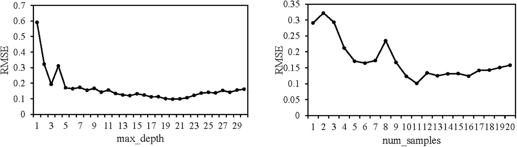
Figure 2. Sensitivity of CART parameters on the RMSE.

TABLE 3

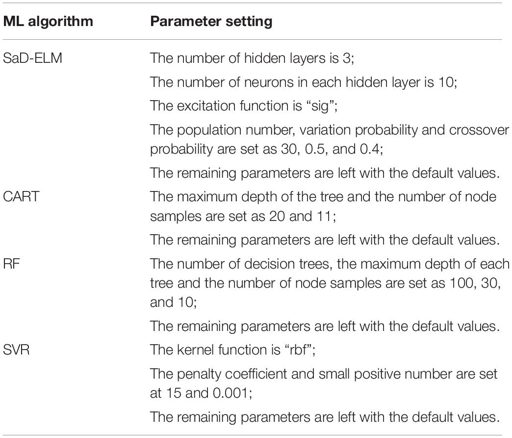
Table 3. Parameter setting of four ML algorithms.

After training the parameters of the ML models, we input testing samples for prediction. Ten sets of training samples and testing samples are used in turn to perform SIC prediction experiments. The model performance is evaluated by quantitatively comparing the prediction results based on three accuracy metrics: RMSE, R and MRE.

(5) Evaluation of Different Input Variables

We conduct the SIC prediction experiment (lead time = 1 d) in the Kara Strait with different predictor variables. The accuracy metrics of each experimental results are presented in Figure 3. As can be seen from the figures, for the four ML models, the metrics of each experimental result have little difference, indicating the performance of the ML-based prediction models is stable for different testing sets.

FIGURE 3

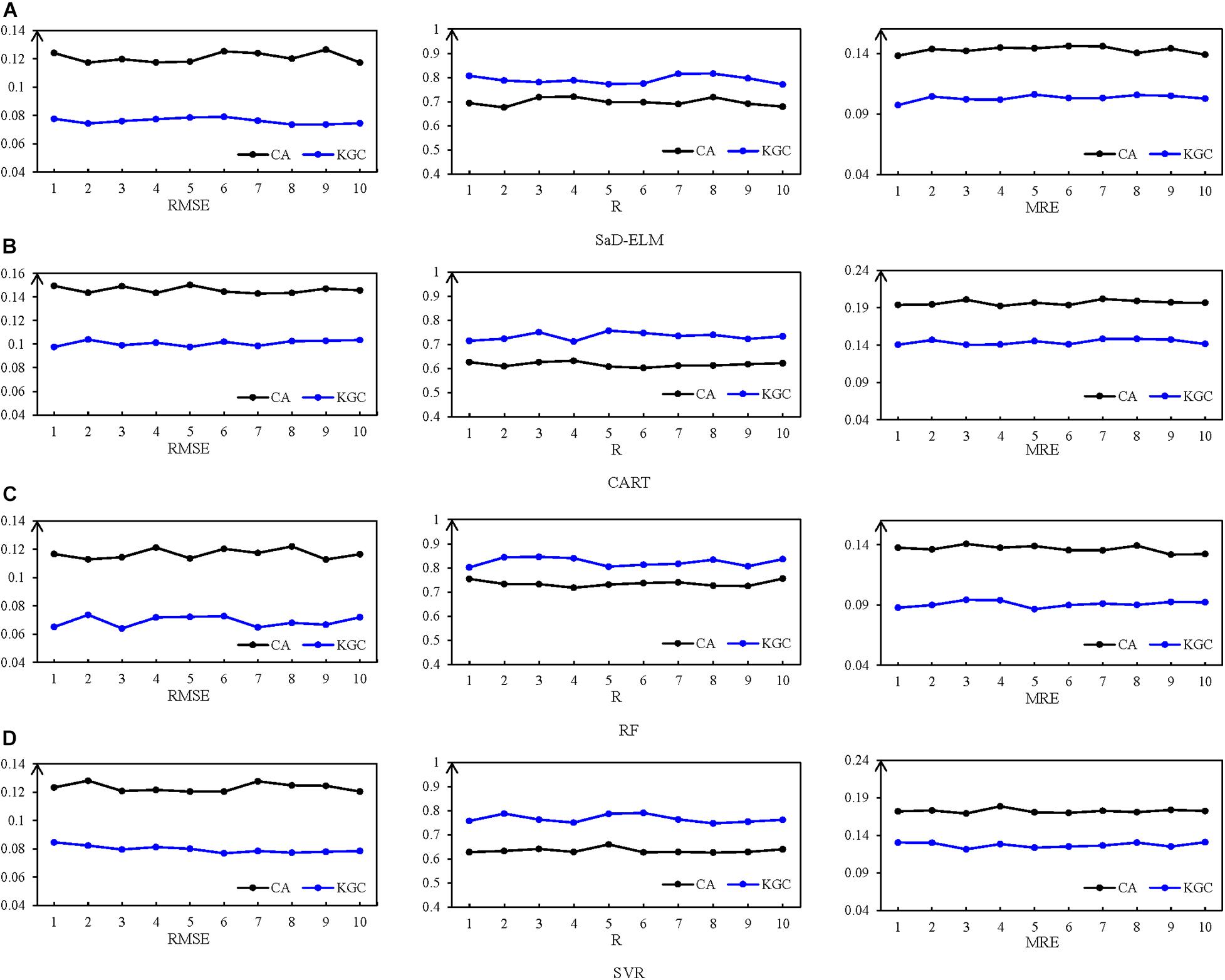
Figure 3. RMSE, R, and MRE of the four prediction model with the 10-fold cross-validation. (A) SaD-ELM. (B) CART. (C) RF. (D) SVR.

For further analysis, we calculate the average of ten prediction results as the final result, which is displayed in Figure 4. RMSE, R and MRE of the results are shown in Figure 5 and Table 4. From visual inspection in Figure 4, for the four ML models, it appears that the predicted trends with input variables screened out by causal analysis are significantly better than predictions based on correlation analysis. It can be seen from Figure 5 that, although prediction performances of four causal analysis-based ML models are different, it is worth noting that RMSE is less than 0.1, R is greater than 0.7, and MRE is less than 0.15, better than the climatology used as the benchmark (RMSE: 0.113, R: 0.689, MRE: 0.172). Compared with correlation analysis, predicted results (Table 4) with causal analysis selecting predictors are improved dramatically: on average, RMSE decreases by 36.15%, R increases by 16.09% and MRE decreases by 29.17%. To sum up, ML models with input factors screened by causal analysis have a significantly better prediction performance than those based on correlation analysis. Causal analysis is an effective predictor screening method.

FIGURE 4

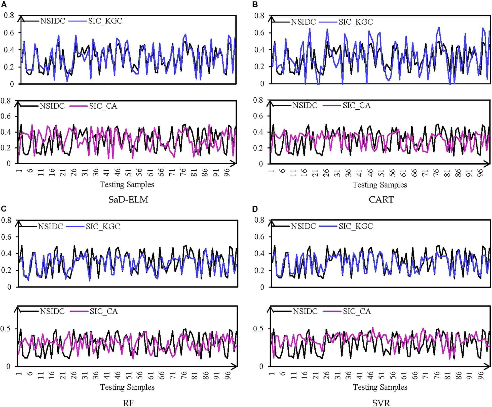
Figure 4. Mean prediction with lead time = 1 day of (A) SaD-ELM, (B) CART, (C) RF, and (D) SVR. The black line represents the observed SIC of NISIDC; the blue line represents the prediction based on causal analysis; and the red line represents the prediction based on correlation analysis.

FIGURE 5

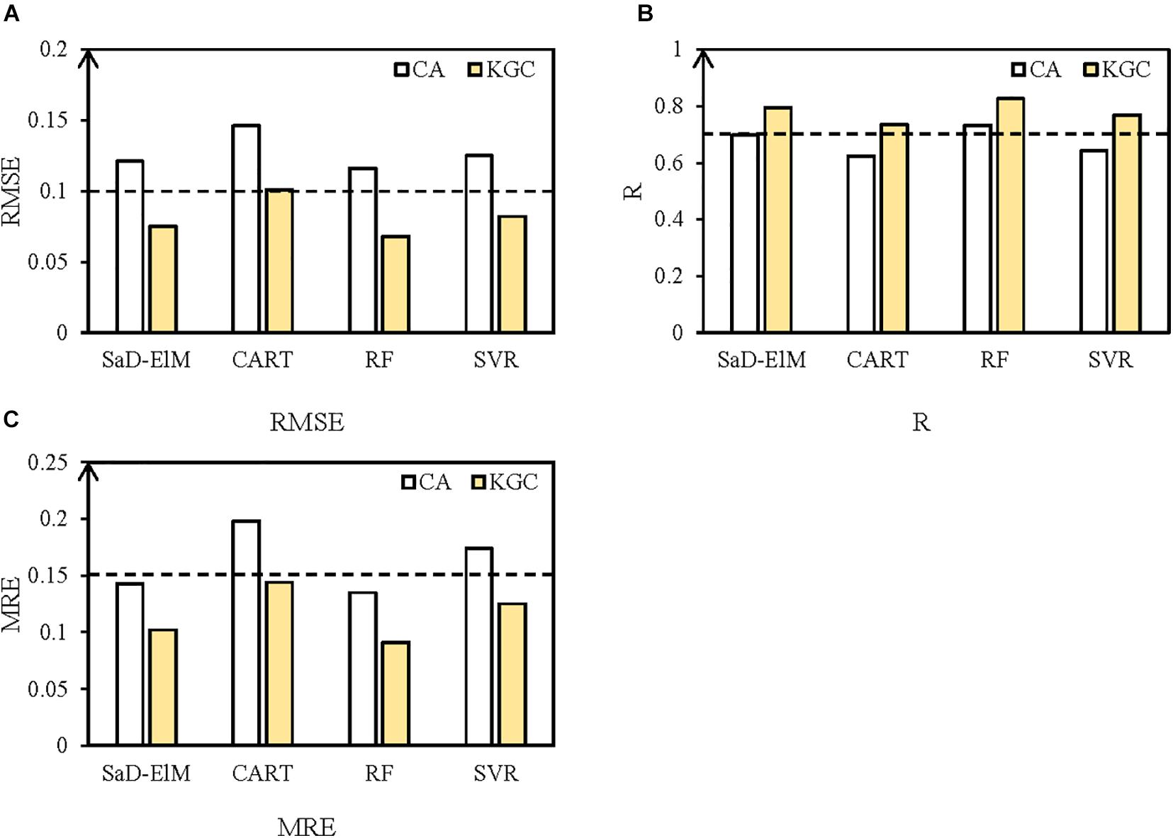
Figure 5. (A) R, (B) RMSE, and (C) MRE of mean predicted SIC with different prediction models. White represents the prediction based on correlation analysis; yellow represents the prediction based on causal analysis.

TABLE 4

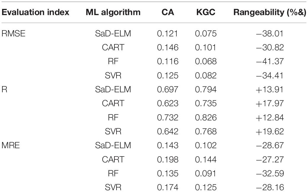
Table 4. RMSE, R, and MRE of SIC prediction with different predictors.

(6) Evaluation of Various Lead Times

Then we take predictors screened by KGC to build ML-based prediction models for SIC prediction with different lead times (1, 3, and 5 d). RMSE, R, and MRE of predicted results are showed in Table 5 and Figure 6.

TABLE 5

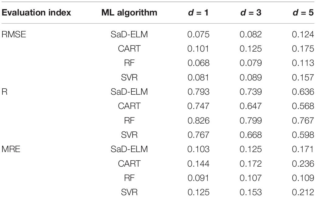
Table 5. Predicted results with different ML algorithms and lead times.

FIGURE 6

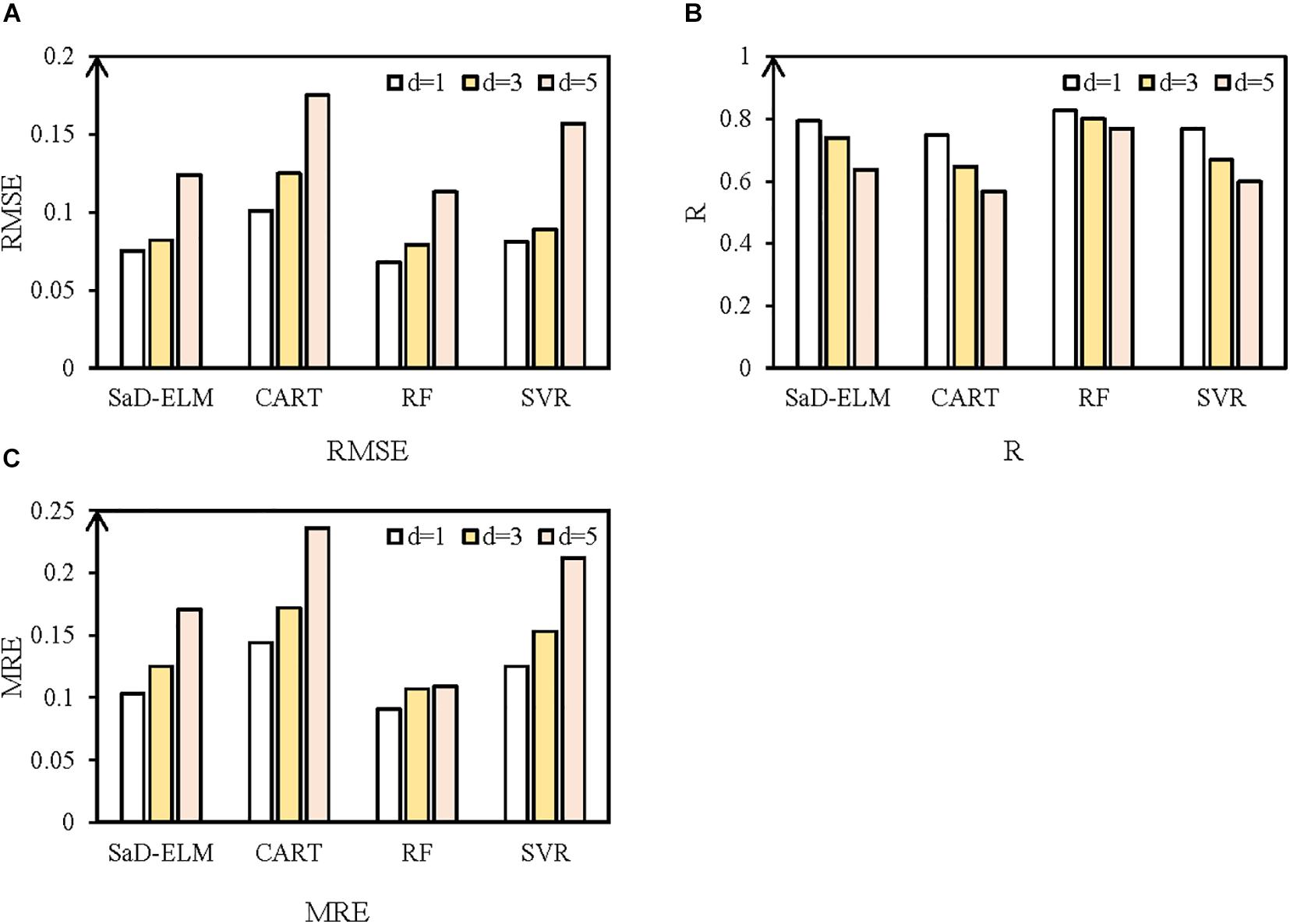
Figure 6. Predicted results with different ML algorithms and lead times. (A) RMSE. (B) R. (C) MRE. White represents prediction in lead time = 1 day; yellow represents prediction in lead time = 3 days; and pink represents prediction in lead time = 5 days.

It can be seen from Table 5 that, for different lead times, the prediction performance of CART is the worst, perhaps because CART is often used to process discrete data and is prone to overfitting for continuous time series prediction. In addition, SVR is better than CART, but slightly worse than SaD-ELM and RF, perhaps because daily time series of SIC contain some noise and SVR is sensitive to data noise (Liu et al., 2020), so the prediction error brought by noise increases. By contrast, SaD-ELM based on adaptive differential evolution and RF based on ensemble learning mechanism can obtain more accurate prediction for different lead times.

Figure 6 illustrates that, with the increase of lead time, the prediction performances of the four ML models decrease to a greater or lesser degree: the prediction accuracy of CART and SVR decreases notably; RF is the most stable, perhaps because RF is an ensemble learning algorithm based on CART, which can reduce the possibility of overfitting through averaging DTs, so it is more accurate and stable than one individual model. When lead time is short (<3 d), all the four ML models can achieve satisfactory predicted results. That is because the relationships between adjacent time are close with short lead time and the nonlinearity is weak, so the mapping between predictors and SIC can be easily captured by all ML algorithms. With lead time increasing, SaD-ELM and RF still maintain stable prediction accuracy, while the accuracy of CART and SVR decreases dramatically. The error feed-back loop in SaD-ELM achieves the automatic error correction and the ensemble learning mechanism in RF can enhance the prediction effect through multi model fusion modeling. Therefore, SaD-ELM and RF perform better with long lead time. Through the prediction experiment of SIC in the Kara Strait, it can be concluded that: (1) Compared with correlation analysis, the input factors of ML models screened out by causal analysis lead to better predicted results; (2) By analyzing R, RMSE, and MRE, the four ML algorithms are all suitable for short-term prediction of SIC. Thereinto, RF and SaD-ELM have better prediction performance under long lead time condition.

Experiment II: SIC Prediction in the B-K Sea (70–80°N, 20–80°E)

In order to test the generalization ability of various ML algorithms and further discuss the reliability of ML, we also make a short-term prediction of SIC fields in the whole B-K sea. Based on the predictor variables selected by causal analysis, four ML-based prediction models are constructed to predict daily spatial distribution of SIC. At present, the studies about spatial field prediction using ML algorithms are the minority. In our research, we build the prediction model grid by grid in the spatial field.

The data processing and parameters setting are carried out by the same processes in Experiment I, and the remaining 100 samples of each grid point are used for the model test. Figure 7 shows the predicted results (lead time = 1d) of SIC at grid point (80°E, 80°N). The distribution map of RMSE and R in the B-K sea are shown in Figures 8, 9.

FIGURE 7

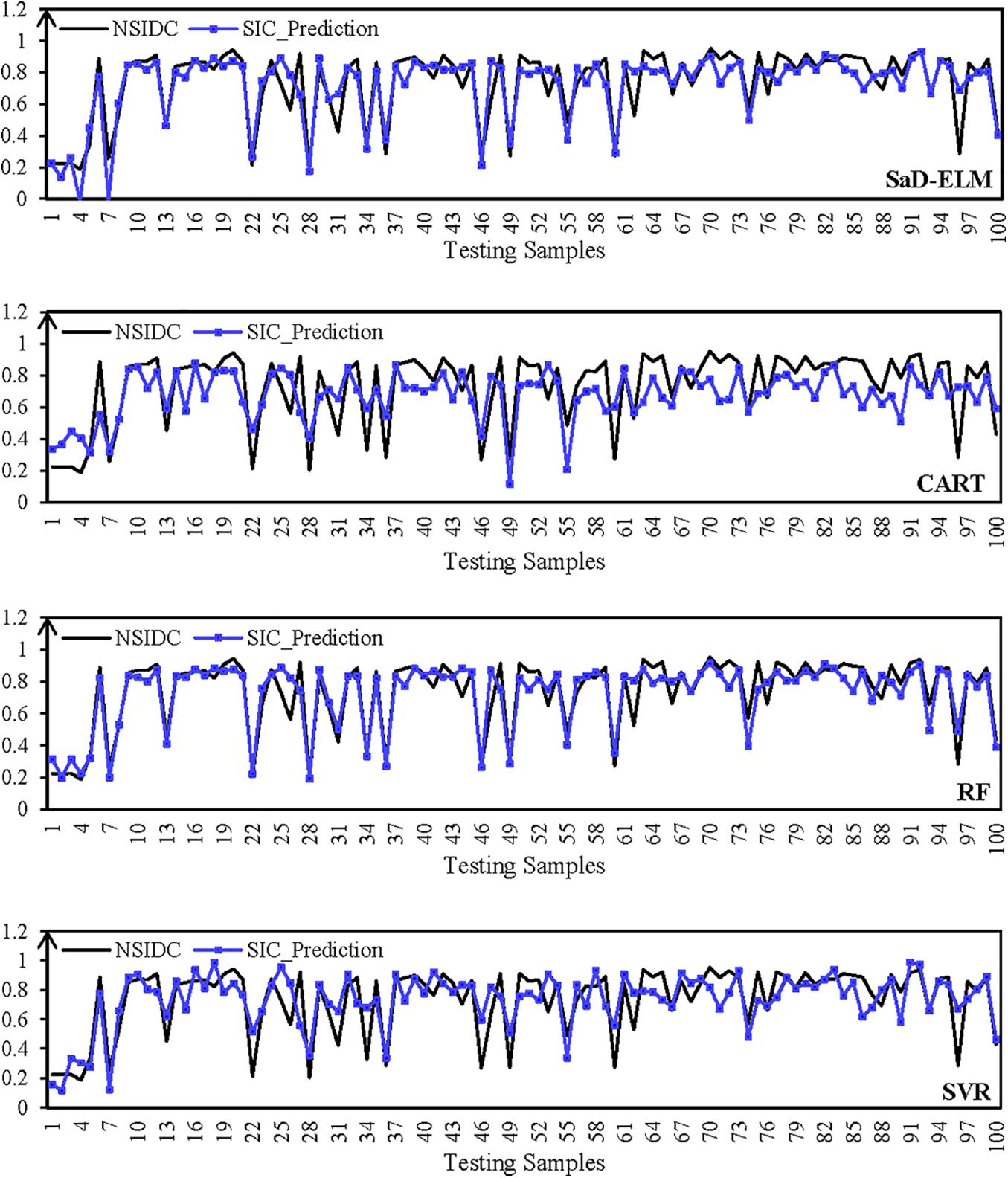
Figure 7. Predicted SIC at grid point (80°E, 80°N) (the black line represents the observed SIC of NISIDC; the blue line represents the predicted SIC in lead time = 1 d).

FIGURE 8

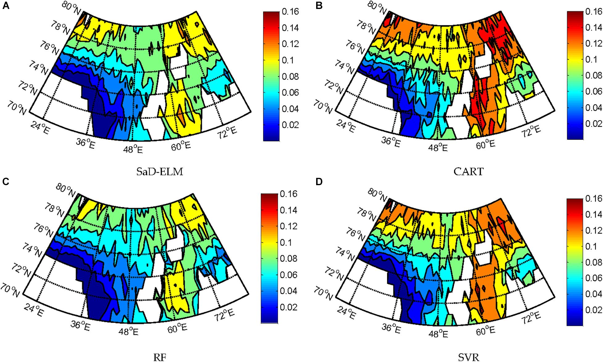
Figure 8. RMSE of predicted SIC at each grid point of B-K sea with four models (lead time = 1 day). (A) SaD-ELM. (B) CART. (C) RF. (D) SVR.

FIGURE 9

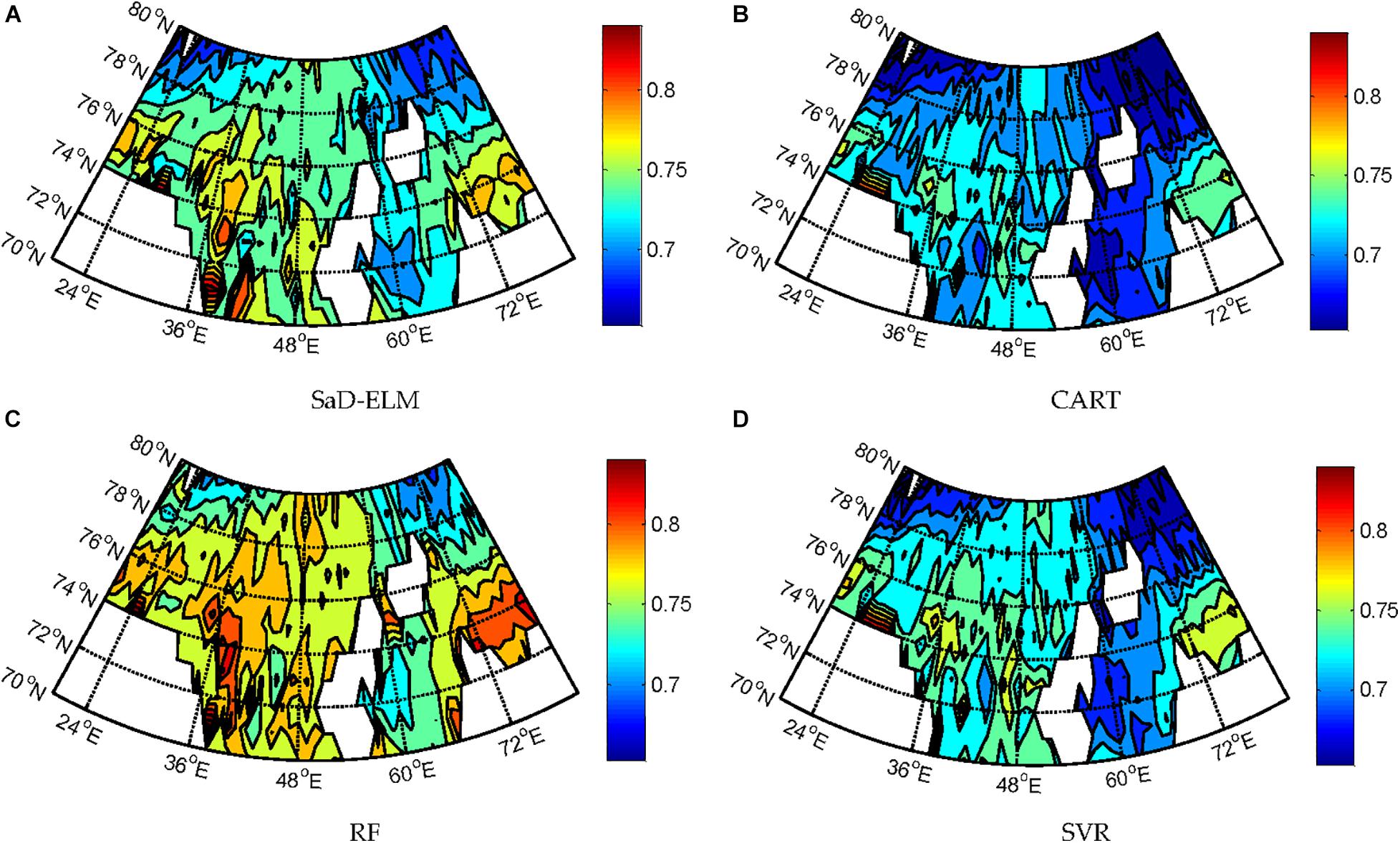
Figure 9. R of predicted SIC at each grid point of B-K sea with four models (lead time = 1 day). (A) SaD-ELM. (B) CART. (C) RF. (D) SVR.

It can be seen from Figure 7: when lead time = 1d, all ML algorithms can achieve effective prediction of SIC at different sites. The predicted peak/low value corresponds to the observation, and the changing trend of each time series is accurately expressed. Prediction performances of SaD-ELM and RF are better than CART and SVR, which is consistent with the conclusion obtained in Experiment I. Figure 8 displays that the prediction errors of the four ML algorithms in different regions of the B-K sea are significantly different. From visual inspection, RMSE of predicted SIC in the Kara Sea is higher than that in the Barents Sea. We speculate that Novae Island and Eurasia continent, surrounding the Kara sea, may affect the result as land can lead to local meteorology and marine environment more complex and changeable. Therefore, the sea ice is susceptible to change and SIC is more difficult to predict (Chevallier et al., 2013; Liu et al., 2020).

To determine the prediction ability of ML algorithms, we calculate the average of each performance measure for all grid points (61 × 11) and estimate the computational complexity. Table 6 shows that, when lead time is short (<3d), the prediction accuracy of these ML algorithms is satisfactory, better than the accuracy of climatology, and suitable for SIC prediction. RF based on ensemble learning has the highest prediction accuracy, followed by SaD-ELM and SVR, while CART has the worst prediction performance. From the perspective of model running time, although the prediction performance of SaD-ELM is slightly less than RF, its running time is shorter. In light of this advantage, SaD-ELM can be applied to real-time or quasi real-time sea ice prediction, which is of great significance to Arctic navigation and engineering management. By contrast, RF and SVR have lower performance when it comes to computational complexity, which implies poor practical engineering application.

TABLE 6

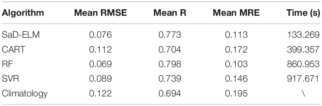
Table 6. Mean RMSE, R, MRE, and model running time of different prediction models (lead time = 1 d).

In addition, we further compare the generalization ability of the four ML algorithms. We take new datasets of predictors and SIC from January 1st to June 30th, 2000 as testing samples and predict SIC (lead time = 1d) with the trained ML-based prediction models in section “Experiment II: SIC prediction in the B-K sea (70–80°N, 20–80°E).” Compared with predicted results in Table 6, the prediction accuracy of four ML algorithms is reduced to a certain extent. Table 7 shows that the reduction in prediction accuracy of RF is minimal (RMSE: +36.37%, R: −10.77%, MRE: +21.97%), while the prediction accuracy of SaD-ELM (RMSE: +96.05%, R: −18.89%, MRE: +89.38%) and CART (RMSE: +64.29%, R: −13.92%, MRE: +47.09%) decreases obviously. These results imply that RF has the best generalization ability, followed by SVR, while SaD-ELM performs worse in generalization.

TABLE 7

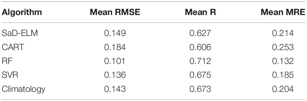
Table 7. Predictions of SIC from January 1st to June 30th, 2000 (lead time = 1 d).

Conclusion

In this article, we put forward a new idea of short-term prediction of sea ice by introducing ML algorithms and causal analysis to prediction modeling. Aiming at the imperious demand of short-term and fast prediction of sea ice in the Arctic navigation, a data-driven prediction technique of SIC based on causal analysis and ML is developed. We first select predictor variables with causal analysis instead of classical correlation analysis, then adopt SaD-ELM, CART, RF, and SVR to establish corresponding prediction models. The applicability and reliability of ML algorithms in sea ice prediction are discussed. The main conclusions are as follows:

(1) Compared with correlation analysis, input variables of ML-based prediction models screened out by causal analysis lead to more accuracy predicted results. Causal analysis works better than correlation analysis in predictor selection.

(2) When lead time is short (<3 d), the four ML algorithms are all suitable for short-term prediction of SIC. With the increase of lead time, although the prediction accuracy of the four models decreases to different degrees, they are adequate to the need for navigation. RF has the best predictive performance, followed by SaD-ELM and SVR, while CART has the worst prediction accuracy.

(3) Compared with CART and SVR, the prediction accuracy of SaD-ELM and RF is more stable with different lead times. RF has the best prediction accuracy and generalization ability but the largest time consuming. SaD-ELM obtains more favorable performance from the aspect of computational complexity but in the meantime, it has weak generalization capability.

Through multi-set of prediction experiments, we analyzed the prediction performance of SaD-ELM, CART, RF, and SVR in SIC prediction at day time scales and concluded that ML algorithms are appropriate for short-term prediction of SIC. However, we only conducted a comparative analysis of multiple ML algorithms, and did not touch on improving the models. Our future research will focus on the optimization of ML-based models to further improve the prediction accuracy of sea ice. In addition, in allusion to the high nonlinearity of the daily time series of SIC, we will preprocess the time series by wavelet decomposition or empirical mode decomposition in the next study.

Data Availability Statement

The original contributions presented in the study are included in the article/supplementary material, further inquiries can be directed to the corresponding author/s.

Author Contributions

ML and RZ conceived and designed the experiments. ML collected the data, performed the experiments, and wrote the manuscript. ML and KL analyzed the data. All authors contributed to the article and approved the submitted version.

Funding

This work was supported by the National Natural Science Foundation of China (Nos. 41976188, 41775165, and 51609254) and the Graduate Research and Innovation Project of Hunan Province (CX20200009).

Conflict of Interest

The authors declare that the research was conducted in the absence of any commercial or financial relationships that could be construed as a potential conflict of interest.

Footnotes

1. ^ https://github.com/danielemarinazzo/KernelGrangerCausality
2. ^ https://nsidc.org/data/g02202/versions/3
3. ^ https://apps.ecmwf.int/datasets/data

References

Bai, C., Zhang, R., and Bao, S. (2017). Forecasting the tropical cyclone genesis over the northwest pacific through identifying the causal factors in the cyclone-climate interactions. J. Atmos. Oceanic Technol. 35, 247–259. doi: 10.1175/jtech-d-17-0109.1

CrossRef Full Text | Google Scholar

Cao, J., Lin, Z., and Huang, G. B. (2012). Self-adaptive evolutionary extreme learning machine. Neural Process. Lett. 36, 285–305. doi: 10.1007/s11063-012-9236-y

CrossRef Full Text | Google Scholar

Chen, D., and Yuan, X. (2004). A markov model for seasonal forecast of Antarctic Sea Ice. J. Clim. 17, 3156–3168. doi: 10.1175/1520-0442(2004)017<3156:ammfsf>2.0.co;2

CrossRef Full Text | Google Scholar

Chevallier, M., Salas y Mélia, D., and Voldoire, A. (2013). Seasonal forecasts of the pan-Arctic sea ice extent using a GCM-based seasonal prediction system. J. Clim. 26, 6092–6104. doi: 10.1175/jcli-d-12-00612.1

CrossRef Full Text | Google Scholar

Chevallier, M., Salasymelia, D., and Germe, A. (2015). “Seasonal forecasts of the sea ice cover in Arctic ocean and subbasins: hindcast experiments with a coupled atmosphere-ocean GCM,” in IEEE International Conference on Intelligent Systems & Control, Piscataway, NJ: IEEE.

Google Scholar

Chi, J., and Kim, H. (2017). Prediction of Arctic Sea Ice concentration using a fully data driven deep neural network. Remote Sens. 9:1305. doi: 10.3390/rs9121305

CrossRef Full Text | Google Scholar

Cvijanovic, I., and Caldeira, K. (2015). Atmospheric impacts of sea ice decline in CO2 induced global warming. Clim. Dyn. 44, 1173–1186. doi: 10.1007/s00382-015-2489-1

CrossRef Full Text | Google Scholar

Deser, C., and Teng, H. (2008). Evolution of Arctic sea ice concentration trends and the role of atmospheric circulation forcing, 1979–2007. Geophys. Res. Lett. 35:L02504.

Google Scholar

Drobot, S. D., Maslanik, J. A., and Fowler, C. (2006). A long-range forecast of Arctic summer sea-ice minimum extent. Geophys. Res. Lett. 331, 229–243.

Google Scholar

Drobot, S. D., and Maslanik, J. A. (2002). A practical method for long-range forecasting of ice severity in the Beaufort Sea. Geophys. Res. Lett. 29:54-1–54-1.

Google Scholar

Fang, Z., and Wallace, J. M. (1994). Arctic sea ice variability on a timescale of weeks and its relation to atmospheric forcing. J. Clim. 7, 1897–1914. doi: 10.1175/1520-0442(1994)007<1897:asivoa>2.0.co;2

CrossRef Full Text | Google Scholar

Gascard, J. C., Riemann-Campe, K., Gerdes, R., Schyberg, H., Randriamampianina, R., Karcher, M., et al. (2017). Future sea ice conditions and weather forecasts in the Arctic: implications for Arctic shipping. Ambio 46, 355–367. doi: 10.1007/s13280-017-0951-5

PubMed Abstract | CrossRef Full Text | Google Scholar

Gong, T., and Luo, D. (2017). Ural blocking as an amplifier of the Arctic sea ice decline in winter. J. Clim. 30, 2639–2654. doi: 10.1175/jcli-d-16-0548.1

CrossRef Full Text | Google Scholar

Granger, C. W. J. (1969). Investigating causal relations by econometric models and cross-spectral methods. Econometrica 37, 424–438. doi: 10.2307/1912791

CrossRef Full Text | Google Scholar

Guemas, V., Blanchard-Wrigglesworth, E., and Chevallier, M. (2016). A review on Arctic sea-ice predictability and prediction on seasonal to decadal time-scales. Q. J. Roy. Meteorol. Soc. 142, 546–561. doi: 10.1002/qj.2401

CrossRef Full Text | Google Scholar

Kang, D., Im, J., Lee, M. I., and Quackenbush, L. J. (2014). The MODIS ice surface temperature product as an indicator of sea ice minimum over the Arctic Ocean. Remote Sens. Environ. 152, 99–108. doi: 10.1016/j.rse.2014.05.012

CrossRef Full Text | Google Scholar

Kim, J., Kim, K., Cho, J., Kang, Y., Yoon, H.-J., and Lee, Y.-W. (2019). Satellite-based prediction of Arctic Sea ice concentration using a deep neural network with multi-model ensemble. Remote Sens. 11:19. doi: 10.3390/rs11010019

CrossRef Full Text | Google Scholar

Krakovská, A., Jakubík, J., Chvosteková, M., Coufal, D., Jajcay, N., Paluš, M., et al. (2018). Comparison of six methods for the detection of causality in a bivariate time series. Phys. Rev. E 97:042207.

Google Scholar

Li, M., and Liu, K. F. (2018). Application of intelligent dynamic Bayesian network with wavelet analysis for probabilistic prediction of storm track intensity index. Atmosphere 9, 224–236. doi: 10.3390/atmos9060224

CrossRef Full Text | Google Scholar

Li, M., and Liu, K. F. (2019). Causality-based attribute weighting via information flow and genetic algorithm for naive bayes classifier. IEEE Access 7, 150630–150641. doi: 10.1109/access.2019.2947568

CrossRef Full Text | Google Scholar

Li, M., and Liu, K. F. (2020). Probabilistic prediction of significant wave height using dynamic bayesian network and information flow. Water 12:2075. doi: 10.3390/w12082075

CrossRef Full Text | Google Scholar

Li, Z., Ringsberg, J. W., and Rita, F. (2019). A voyage planning tool for ships sailing between Europe and Asia via the Arctic. Ships Offshore Struct. 15(Suppl.1), S10–S19.

Google Scholar

Liang, X. S. (2014). Unraveling the cause-effect relation between time series. Phys. Rev. E 90:052150.

Google Scholar

Lindsay, R. W., Zhang, J., Schweiger, A. J., and Steele, M. A. (2008). Seasonal predictions of ice extent in the Arctic Ocean. J. Geophys. Res. Oceans 113:C02023.

Google Scholar

Liu, K., He, Q., and Jing, C. (2020). Gap filling method for evapotranspiration based on machine learning. J. Hohai Univ. 2, 109–115.

Google Scholar

Mahajan, S., Zhang, R., and Delworth, T. L. (2011). Impact of the Atlantic meridional overturning circulation (AMOC) on Arctic surface air temperature and sea ice variability. J. Clim. 24, 6573–6581. doi: 10.1175/2011jcli4002.1

CrossRef Full Text | Google Scholar

Marinazzo, D., Pellicoro, M., and Stramaglia, S. (2008). Kernel method for nonlinear Granger causality. Phys. Rev. Lett. 100:144103.

Google Scholar

Marlene, K., Dim, C., Donges, J. F., and Runge, J. (2016). Using Causal Effect Networks to Analyze Different Arctic Drivers of Midlatitude Winter Circulation. J. Clim. 29:160303130523003.

Google Scholar

McGraw, M. C., and Barnes, E. A. (2020). New Insights on Subseasonal Arctic–Midlatitude causal connections from a regularized regression model. J. Clim. 33, 213–228. doi: 10.1175/jcli-d-19-0142.1

CrossRef Full Text | Google Scholar

Mitchell, B., Msadek, R., and Winton, M. (2017). Skillful regional prediction of Arctic sea ice on seasonal timescales. Geophys. Res. Lett. 44, 4953–4964. doi: 10.1002/2017GL073155

CrossRef Full Text | Google Scholar

Poggio, T. A., Weston, J., and Mukherjee, S. (2000). Feature Selection for SVMs. Boston, MA: MIT Press.

Google Scholar

Rayner, N. A. A., Parker, D. E., and Horton, E. B. (2003). Global analyses of sea surface temperature, sea ice, and night marine air temperature since the late nineteenth century. J. Geophys. Res. Atmos. 108:4407.

Google Scholar

Runge, J., Bathiany, S., Bollt, E., Camps-Valls, G., Coumou, D., Deyle, E., et al. (2019). Inferring causation from time series in Earth system sciences. Nat. Commun. 10:2553.

Google Scholar

Schweiger, A. J., and Zhang, J. (2015). Accuracy of short-term sea ice drift forecasts using a coupled ice-ocean model. J. Geophys. Res. Ocean 120, 7827–7841. doi: 10.1002/2015jc011273

PubMed Abstract | CrossRef Full Text | Google Scholar

Screen, J. A., and Simmonds, I. (2010). The central role of diminishing sea ice in recent Arctic temperature amplification. Nature 464, 1334–1337. doi: 10.1038/nature09051

PubMed Abstract | CrossRef Full Text | Google Scholar

Screen, J. A., Simmonds, I., Deser, C., and Tomas, R. (2013). The atmospheric response to three decades of observed Arctic sea ice loss. J. Clim. 26, 1230–1248. doi: 10.1175/jcli-d-12-00063.1

CrossRef Full Text | Google Scholar

Shimada, K., Kamoshida, T., Itoh, M., Nishino, S., Carmack, E., McLaughlin, F., et al. (2006). Pacific Ocean inflow: influence on catastrophic reduction of sea ice cover in the Arctic Ocean. Geophys. Res. Lett. 33:L08605.

Google Scholar

Sims, C. A. (1972). Money, income, and causality. Am. Econ. Rev. 62, 540–552.

Google Scholar

Stroeve, J., Hamilton, L. C., Bitz, C. M., and Blanchard−Wrigglesworth, E. (2014). Predicting September sea ice: ensemble skill of the search sea ice outlook 2008–2013. Geophys. Res. Lett. 41, 2411–2418. doi: 10.1002/2014gl059388

CrossRef Full Text | Google Scholar

Stroeve, J., Serreze, M., and Drobot, S. (2008). Arctic sea ice extent plummets in 2007. Eos Trans. Am. Geophys. Union 89, 13–14. doi: 10.1029/2008eo020001

CrossRef Full Text | Google Scholar

Sugihara, G., May, R., Ye, H., Hsieh, C. H., Deyle, E., Fogarty, M., et al. (2012). Detecting causality in complex ecosystems. Science 338, 496–500. doi: 10.1126/science.1227079

PubMed Abstract | CrossRef Full Text | Google Scholar

Wang, L., Scott, K., and Clausi, D. (2017). Sea ice concentration estimation during freeze-up from SAR imagery using a convolutional neural network. Remote Sens. 9:408. doi: 10.3390/rs9050408

CrossRef Full Text | Google Scholar

Wang, L., Yuan, X., Ting, M., and Li, C. (2016). Predicting summer Arctic Sea Ice concentration intraseasonal variability using a vector autoregressive model. J. Clim. 29, 1529–1543. doi: 10.1175/jcli-d-15-0313.1

CrossRef Full Text | Google Scholar

Yuan, X., Chen, D., Li, C., Wang, L., and Wang, W. (2016). Arctic sea ice seasonal prediction by a linear markov model. J. Clim. 29, 8151–8173. doi: 10.1175/jcli-d-15-0858.1

CrossRef Full Text | Google Scholar

Zhang, D. Y., Yu, S. S., Wang, Y., and Yue, Q.-J. (2017). Sea ice management for oil and gas platforms in the Bohai Sea. Po. Mar. Res. 24(Suppl. 2), 195–204. doi: 10.1515/pomr-2017-0083

CrossRef Full Text | Google Scholar