Ocean Surface Flux Algorithm Effects on Earth System Model Energy and Water Cycles

Earth system models parameterize ocean surface fluxes of heat, moisture, and momentum with empirical bulk flux algorithms, which introduce biases and uncertainties into simulations. We investigate the atmosphere and ocean model sensitivity to algorithm choice in the Energy Exascale Earth System Model (E3SM). Flux differences between algorithms are larger in atmosphere simulations (where wind speeds can vary) than ocean simulations (where wind speeds are fixed by forcing data). Surface flux changes lead to global scale changes in the energy and water cycles, notably including ocean heat uptake and global mean precipitation rates. Compared to the control algorithm, both COARE and University of Arizona (UA) algorithms reduce global mean precipitation and top of atmosphere radiative biases. Further, UA may slightly reduce biases in ocean meridional heat transport. We speculate that changes seen here, especially in the ocean, could be even larger in coupled simulations.

1. Introduction

Ocean surface fluxes of heat, moisture, and momentum control the ocean's impact on weather and climate. Despite many years of field studies, data set development and parameterization improvements, available data sets still do not close the surface energy budget (L'Ecuyer et al., 2015) and uncertainties in fluxes are too large to detect trends (Rhein et al., 2013). The methods used to calculate ocean surface turbulent fluxes are a significant contributor to surface energy budget uncertainties. While the methodological contribution to observational products has been acknowledged and fairly well-explored (e.g., Yu, 2019), the contribution to the spread of Earth system models is not well-understood. In this study we use atmosphere and ocean model simulations to quantify how sensitive model results are to surface flux algorithm design.

The methods used to calculate ocean surface turbulent fluxes in numerical models and global observational products rely on bulk flux algorithms. These algorithms use “bulk” quantities—sea surface temperature (SST) and near-surface values of air temperature, humidity, and wind speed—which are easier to measure than direct measurements of fluxes (e.g., Edson et al., 1998), and can be measured by remote sensing platforms. Bulk algorithms have been compared by Zeng et al. (1998), Brunke et al. (2002, 2003), and Brodeau et al. (2016), among others. While these studies are valuable for understanding how different aspects of algorithm design affect surface flux estimates, they have one limitation when it comes to understanding impacts on model results: they are based on comparison of fluxes using pre-specified bulk variables. Thus, the differences in fluxes do not feed back onto the bulk variables. Therefore, such studies do not allow us to fully understand the changes that result when the algorithms are used in ocean and atmosphere general circulation models, in which case the flux differences do result in changes in the bulk variables. Understanding these feedbacks is key to assessing the full model sensitivity to algorithm choice.

A number of past studies give strong evidence suggesting that model sensitivity to ocean surface flux calculation is significant and important. Looking at the atmospheric response, Harrop et al. (2018) found that tropical Pacific precipitation biases in the Energy Exascale Earth System Model (E3SM) are reduced by including the effects of convective wind gustiness in flux calculations. Large and Caron (2015), building on the work of Zeng and Beljaars (2005), showed that parameterizing diurnal variation of SST in a global atmosphere model can affect net ocean surface heat flux and precipitation. Polichtchouk and Shepherd (2016) showed that the effects of changing the ocean surface roughness formulation in a global model are apparent across the globe and through the full depth of the troposphere. Compared to atmosphere models, the sensitivity of ocean models to surface flux algorithms is comparatively unexplored. However, it has been shown (Holdsworth and Myers, 2015; Kostov et al., 2019) that surface heat flux specification is important for simulating the Atlantic Meridional Overturning Circulation (AMOC). These studies provide motivation for asking what other aspects of ocean model behavior may be sensitive to surface flux algorithm choice.

Given the wide ranging aspects of model climate (i.e., the main features of the simulated Earth system) that are affected by flux calculation methods, and the large number of studies that compare bulk flux algorithms using pre-specified bulk variable data, it is surprising that there are not more studies investigating the consequences of bulk flux algorithm choice in global models—especially in ocean models. We aim to fill this gap, and identify three major aims in doing so:

1. Identify regions where differences between fluxes are largest. This will assist developers of parameterizations to understand uncertainties and identify strengths and weaknesses. Given the uncertainties in observation-based flux data sets (Găinuşă-Bogdan et al., 2015), it is difficult to identify a “least biased” parameterization. Instead we aim to identify where the differences between algorithms are significant, based on the what might be expected from internannual and longer term variability. Regions with significant differences can then be prioritized for more detailed regional process studies and analysis of structural differences in the algorithms.

2. Understand how the choice of test methodology (atmosphere vs. ocean simulations) affects the apparent outcome. Due to their different forcing data requirements, atmosphere and ocean simulations allow different amounts of flux-bulk variable feedback. Strobach et al. (2018) showed that inclusion or exclusion of such feedbacks has a large impact on ocean model simulations, and similar issues likely affect atmosphere-only simulations. Thus, our work will help modelers and parameterization developers to understand how the choice of testing framework may influence results.

3. Explore which other aspects of model climate are affected, to help model developers understand how surface flux parameterization may influence the perceived biases of the overlying atmosphere and/or underlying ocean model(s). Based on the studies mentioned above, we expect differences in precipitation, large-scale atmospheric circulation, and possibly in deep water formation at high latitudes. However, changes in other quantities and/or regions are possible.

The structure of this paper is as follows: section 2 summarizes the bulk flux algorithms, model simulations and observational data; section 3 presents results—of both surface fluxes and other aspects of model climate; section 4 includes further discussion and summarizes our findings.

2. Data and Methods

2.1. Bulk Flux Algorithms

Exchanges of heat, moisture and momentum between atmosphere and ocean are calculated in global models using bulk flux algorithms. These algorithms parameterize turbulent fluxes based on bulk quantities: sea surface temperature (SST), near-surface air temperature and humidity, and near-surface wind speed. Bulk flux algorithms have sound theoretical foundations in Monin-Obukhov similarity theory. However, many aspects of the algorithms are empirical, relying on constants and functional forms estimated from (a relatively small number of) ship- and buoy-based observational campaigns. The general form of the flux algorithms can be expressed as:

$\begin{array}{ll}\overrightarrow{\tau }=\rho C_D(\overrightarrow{U_z}-\overrightarrow{U_s})U_B& (1)\end{array}$

$\begin{array}{ll}{Q}_H=\rho c_p{C}_H({\theta }_z-{\theta }_s)U_B& (2)\end{array}$

$\begin{array}{ll}{Q}_E=\rho L_v{C}_E(q_z-q_s)U_B& (3)\end{array}$

where $\overrightarrow{\tau }$ is the wind stress, Q_H is the sensible heat flux, and Q_E is the latent heat flux. The main differences between algorithms lie in the calculation of the transfer coefficients C_D, C_E, and C_H, but there are also differences in U_B (which may simply be the wind speed or may have a modification due to boundary layer eddies or convective gustiness), and even in the calculation of q_s (surface specific humidity) and L_v (latent heat of vaporization). Other terms appearing in the equations are ρ (air density), c_p (specific heat capacity of air), θ (potential temperature), q (specific humidity), and $\overrightarrow{U}$ (wind velocity). Subscript z refers to a value at height z in the atmosphere (in our case, the height of the lowest atmosphere model level), while subscript s refers to the value at the ocean surface. The sign conventions employed mean that $\overrightarrow{\tau }$ is the force exerted on the ocean by the wind, and positive values of Q_H and Q_E correspond to heat gain by the ocean. The coefficients C_D, C_E, and C_H have two main dependencies: stability (turbulence is enhanced in unstable conditions) and surface roughness (the ocean surface becomes rougher at higher wind speeds). Many researchers have proposed different formulations for these coefficients, and the differences in their formulations are responsible for some of the differences between algorithms. In addition, several seemingly more trivial issues (e.g., reduction of surface specific humidity due to ocean salinity; use of constant air density) can strongly affect flux calculations (Brodeau et al., 2016). This study uses three bulk flux algorithms: they are described in detail in the references given, but here (and in Table 1) we summarize some of their key features and differences.

TABLE 1

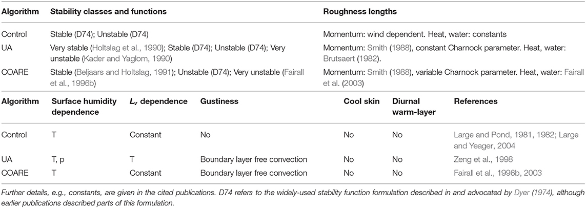
Table 1. Bulk flux algorithm overview.

The first, which we refer to as “control,” is the algorithm used in the Energy Exascale Earth System Model version 1 (E3SMv1 Golaz et al., 2019). It is based on the work of Large and Pond (1981, 1982) and Large and Yeager (2004, 2009). The algorithm uses two stability classes—stable and unstable. The roughness length for momentum varies with wind speed. The roughness length for heat takes one of two constant values depending on stability, while that for moisture uses a single constant for all stability cases. Surface specific humidity is calculated with a simple formula based on temperature only and accounts for reduction due to ocean salinity.

The University of Arizona algorithm (Zeng et al., 1998), which we refer to as “UA,” uses four stability cases (strongly stable, weakly stable, weakly unstable, and very unstable). Roughness lengths for momentum, heat and moisture are continuously varying functions of wind speed. Surface specific humidity uses a more accurate formula than the control algorithm, based on temperature and surface pressure. Again, the reduction due to ocean salinity is accounted for. Similarly, UA uses a temperature-dependent function for L_v, while the other two algorithms use a single constant. Finally, UA includes a gustiness factor due to large boundary layer eddies in unstable conditions, which increases fluxes in unstable, low wind conditions.

The third algorithm is based on the COARE (Coupled Ocean Atmosphere Response Experiment) version 3.0 algorithm (Fairall et al., 2003) which we refer to as simply “COARE.” This uses three stability cases (stable, weakly unstable and strongly unstable) and roughness length functions are similar to the UA algorithm. Surface humidity calculation uses the same method as the control algorithm. COARE, like UA, includes a gustiness factor to account for increased fluxes in unstable, low wind conditions. The correction of sea surface temperature due to cool skin and diurnal warm layer effects available in COARE are not used.

2.2. Model Experiments

We test model sensitivity to ocean surface flux algorithm in a “standard resolution” version of E3SM similar to version 1 used in Golaz et al. (2019). The components of E3SM include atmosphere, land, ocean, sea ice, land ice, and river routing models. The atmosphere and land model horizontal resolutions are ~1° and the ocean and sea ice model horizontal resolutions are ~50 km. The tests performed for this study fall into two categories: one uses active atmosphere and land model components, with sea surface temperature and sea ice distribution pre-specified (this configuration is referred to as an atmosphere run); the other uses active ocean and sea ice components, with near-surface meteorology and river discharge pre-specified (this configuration is referred to as an ocean run). The ocean and sea ice data used in the atmosphere runs is based on a repeating year representative of observations in the year 2000. The atmosphere and river discharge data used in the ocean runs is from the JRA55-do data set (Tsujino et al., 2018)—a version of the JRA-55 reanalysis adjusted to make it more suitable for forcing ocean models.

For each configuration (atmosphere and ocean), three simulations are performed—one with each of the algorithms. The atmosphere runs are 6 years long and analysis is based on the final 5 years. The ocean runs are 10 years long and the first year is disregarded when calculating climatologies but is used for some time series analysis. The ocean runs were originally intended to be the same length as the atmosphere runs, but we took advantage of an opportunity to extend them. Longer model runs would have been valuable, particularly for the ocean model, which can take hundreds to thousands of years to reach equilibrium (Li et al., 2013; Petersen et al., 2019). However, computing resources did not allow for such an ambitious investigation and we feel that the present simulations can still provide a valuable perspective on the degree of sensitivity compared to other model developments (e.g., tuning of parameterizations).

To understand how much of the observed differences between model runs may be due to internal climate variability, we use the E3SM v1 pre-industrial control run (produced for phase 6 of the Coupled Model Intercomparison Project [CMIP6]). We use the final 100 years of the run (model years 401–500) to quantify internal variability.

When analyzing spatial fields, all variables are interpolated onto a common 1° latitude-longitude grid. Heat fluxes and precipitation are interpolated using an integral-conservative method, while wind stress and sea surface height are bilinearly interpolated. We used interpolation tools and several other data processing tools from the netCDF Operators package (Zender, 2020). Global averages are calculated on native model grids.

2.3. Observational Data

Most of the analysis presented here is based on the above model runs, but a few observational data sets are used to contextualize the results. We deem uncertainties in global gridded ocean flux products to be too large to use them for the basis of ranking the flux algorithms (Găinuşă-Bogdan et al., 2015; Yu, 2019). However, we use one such product, OAflux (Yu et al., 2006; Yu and Weller, 2007), to ascertain how the estimated internal variability of E3SM compares with observed variability in the real world. Precipitation from the atmosphere simulations is compared with 1981−2010 long-term averages from GPCP (Global Precipitation Climatology Project; Adler et al., 2003, 2018), a satellite-gauge merged observational data set. Global top of atmosphere (TOA) radiation measurements from the Clouds and the Earth's Radiant Energy System (CERES) mission are used to assess the atmosphere simulations: we use version 4.1 of the energy balanced and filled (EBAF) monthly means (Loeb et al., 2018; Doelling, 2019).

3. Results

We first look at the differences in ocean surface fluxes between model simulations, before looking at the effects on other aspects of model climate in the ocean and atmosphere.

3.1. Surface Flux Changes

Changes in latent heat flux are shown in Figure 1. It is immediately clear that there are differences in sensitivity between atmosphere (left column) and ocean (right column) simulations. The magnitudes of differences are generally larger for atmosphere simulations than for ocean simulations and the spatial patterns differ. However, because the atmosphere simulations have both large positive and large negative differences, there is significant cancellation when considering the global means (Table 2). The sensitivity as shown by the global means therefore ends up being more consistent between atmosphere and ocean tests [e.g., (UA − control) is positive for both atmosphere and ocean].

FIGURE 1

Figure 1. Differences in annual mean latent heat flux climatology between simulations with different bulk flux algorithms. The atmosphere and ocean simulation results are shown in left and right panels, respectively. Stippling designates regions where the absolute value of the difference is larger than the interannual standard deviation from the E3SMv1 pre-industrial control run (shown in Supplementary Figure 2).

TABLE 2

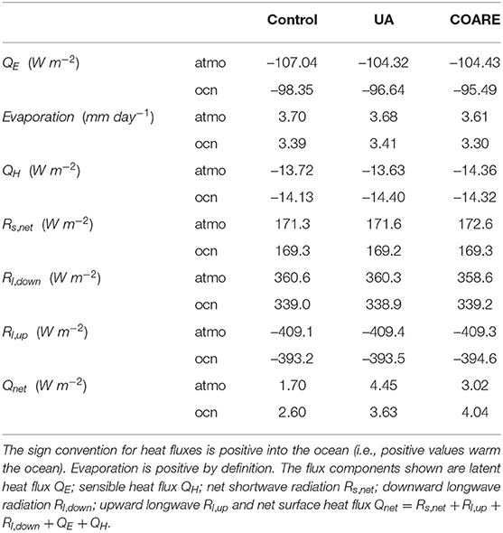
Table 2. Long-term annual mean surface flux components from atmosphere and ocean simulations, averaged over global oceans.

At this point we pause to note that the global means in Table 2 also show latent heat fluxes are of larger magnitude (i.e., more evaporation) in the atmosphere runs than in the ocean runs. However, the physical significance of this fact is doubtful, as the values are likely to be strongly affected by the forcing data sets (Figure 2 and Supplementary Figure 1) and initial conditions, and may even reflect differences introduced by masking and interpolating from different model grids. We therefore do not dwell further on quantitative comparisons between ocean and atmosphere simulations.

FIGURE 2

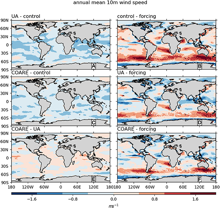
Figure 2. Annual mean 10-m wind speed difference between (left column) pairs of atmosphere model runs and (right column) atmosphere model runs and forcing data used in ocean model runs. The same observation-based wind forcing is used for all three ocean model runs.

Considering the spatial patterns of latent heat flux differences in Figure 1, a few regions stand out that have similar patterns of sensitivity in both the atmosphere and ocean runs. Examples include the Southern Ocean (e.g., around 50°S, 180°E) in COARE − control, and the eastern tropical Pacific (around 5°S, 120°W) in UA−control. Several other regions, however, have opposite changes in the atmosphere and ocean runs. For example, around the Gulf Stream at 35°N, 60°W (a region of large evaporation and therefore negative values in the sign convention of Figure 1) in the UA−control atmosphere comparison, UA has a positive change (less evaporation) relative to control, while in the UA−control ocean comparison, UA has a negative change (more evaporation). Other regions with opposite changes between atmosphere and ocean runs include parts of the North Atlantic Current (40°N, 50°W) and eastern tropical Pacific (5°S, 120°W) in COARE − control, and the Kuroshio (35°N, 140°E) and Agulhas (35°S, 15°E) currents in UA−control.

The regional inconsistencies between atmosphere and ocean simulations bring into question the robustness and significance of the differences shown. We argue below that some of the inconsistency between ocean and atmosphere sensitivity tests arises because the different test methods probe different aspects of the bulk flux algorithms. In the meantime, to address the question of significance, we compare the magnitude of changes to the interannual standard deviation of latent heat flux from the E3SMv1 pre-industrial control run (stippling in Figure 1). In the atmosphere sensitivity tests, large areas of the world's oceans exhibit significant changes. For the ocean tests, however, only a small fraction of ocean areas has significant changes. The chosen significance threshold (E3SMv1 interannual standard deviation) has similar patterns and magnitudes as the interannual standard deviation from the OAflux observational product (Supplementary Figure 2). An alternative significance threshold can be calculated as the range (maximum minus minimum) of 5-year means from the E3SM control run and from OAflux. This results in a larger threshold (Supplementary Figure 2), and therefore would lead to smaller areas of significant changes in Figure 1.

Evaporation differences (Table 2) largely reflect differences in latent heat flux. Thus, global mean evaporation is generally larger in control than in UA or COARE. However, one slight complication in this is that UA uses a temperature-dependent value for the latent heat of evaporation (L_v in Equation 3) while control and COARE both use a single constant. This accounts for the fact that UA has the largest evaporation in the ocean simulations, despite have a smaller magnitude of latent heat flux than control.

Compared to latent heat flux, sensible heat flux (Figure 3) shows greater consistency between sensitivity in atmosphere and ocean simulations. Taking the UA−control comparisons, for example, both the atmosphere and ocean simulations show negative changes across much of the tropics and subtropics and positive changes in parts of the Southern Ocean and North Atlantic. That being said, there are still clear differences. For example, tropical changes for UA−control are smaller (and generally not significant) in the atmosphere tests but are significant in the ocean tests.

FIGURE 3

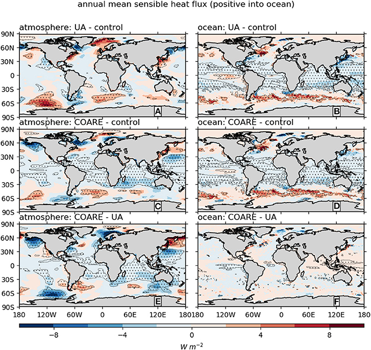
Figure 3. Differences in annual mean sensible heat flux climatology between simulations with different bulk flux algorithms. The atmosphere and ocean simulation results are shown in left and right panels, respectively. Stippling designates regions where the absolute value of the difference is larger than the interannual standard deviation from the E3SMv1 pre-industrial control run. Note that the color scale is different from that in Figure 1.

Comparing across algorithms, we see that similarity between UA and COARE runs is generally greater for sensible heat flux than for latent heat flux (especially in the ocean simulations). This can be seen by noting that Figures 3A,C are quite similar and, to an even greater extent, Figures 3B,D are similar. Relative to this, the pairwise comparisons (A vs. C; B vs. D) in Figure 1 show less similarity. This is in line with the finding of Brunke et al. (2011) who showed that, in observational flux products, latent heat flux uncertainties were dominated by algorithm differences, but sensible heat flux and wind stress uncertainties were dominated by bulk variable differences.

Despite the similarities in patterns of sensible heat flux differences shown in Figure 3, the global averages do not paint a clear picture. For example, in the atmosphere runs COARE has the largest magnitude, while in the ocean runs, UA has the largest magnitude. As a further example, for control and UA, the ocean simulations have larger magnitude sensible heat fluxes than for the atmosphere simulations, while for COARE, the atmosphere simulation has the larger magnitude. It should be noted that the differences in sensible heat flux between algorithms can be the same order of magnitude as differences in latent heat fluxes, even though the sensible fluxes themselves are an order of magnitude smaller.

By changing the sensible and latent heat fluxes, bulk flux algorithms can directly change the ocean surface net heat flux. Further indirect net heat flux changes are possible due to changes in radiation fluxes. In the ocean simulations, SST changes affect upward long wave radiation, though downward long wave and short wave are both specified by the forcing. In the atmosphere simulations, temperature, cloud, and humidity changes affect downward long wave and short wave radiation, though the upward long wave is specified by the forcing (Note that small differences occur in the forcing-specified fields in Table 2 due to sea ice differences). These indirect radiation changes are of similar magnitudes to the latent and sensible heat flux differences. The combined impact of changes in all heat flux components are relatively large, in a relative sense. For example, the UA atmosphere simulation Q_net is more than double that of the control atmosphere simulation, and the COARE ocean simulation Q_net is more than 50% greater than that of the control ocean simulation. The effects of these changes on the atmosphere and ocean model climate are discussed in the following subsections.

We turn next to wind stress sensitivity. For zonal wind stress (Figure 4), ocean and atmosphere tests produce qualitatively similar results. There are, however, differences in the magnitude of changes (especially in midlatitudes) and some regions where sensitivity is of opposite sign in the atmosphere and ocean simulations (mostly in the Southern Ocean, e.g., at 45°S, 0°E). The effects of UA and COARE, relative to the control algorithm, are similar in the ocean simulations: relative to control both UA and COARE cause increased eastward wind stress in midlatitudes and increased westward wind stress in the tropics. Note that this essentially corresponds to UA and COARE giving a larger wind stress than control for any particular wind speed. While the same general pattern holds for the atmosphere simulations, the COARE − UA atmosphere comparison reveals that their patterns are subtly different enough to result in significant differences.

FIGURE 4

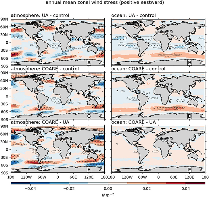
Figure 4. Differences in annual mean zonal wind stress climatology between simulations with different bulk flux algorithms. The atmosphere and ocean simulation results are shown in left and right panels, respectively. Stippling designates regions where the absolute value of the difference is larger than the interannual standard deviation from the E3SMv1 pre-industrial control run.

Finally, for meridional wind stress (Figure 5) ocean and atmosphere tests produce very different results: in atmosphere tests, most of the regions with significant differences are in midlatitudes, while in ocean tests, the significant differences are almost entirely equatorward of 30°. Nonetheless, a few regions show consistent changes across both ocean and atmosphere tests. For example, in the UA-control comparisons, several subtropical marine stratocumulus regions (off the coasts of California, Chile, Namibia, Western Australia) have consistent changes between atmosphere and ocean simulations. The same holds to a lesser degree for the COARE-control comparisons.

FIGURE 5

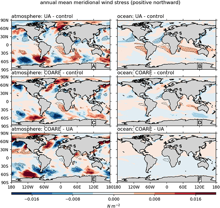
Figure 5. Differences in annual mean meridional wind stress climatology between simulations with different bulk flux algorithms. The atmosphere and ocean simulation results are shown in left and right panels, respectively. Stippling designates regions where the absolute value of the difference is larger than the interannual standard deviation from the E3SMv1 pre-industrial control run. Note that the color scale is different from that in Figure 4.

3.2. Atmosphere Model Sensitivity

The analysis above is mostly concerned with the changes that occur at the ocean surface when using different bulk flux algorithms. We next consider what changes occur in the atmosphere model. We start with precipitation, as this is one of the most important outputs of Earth system models and previous studies (Brunke et al., 2008; Harrop et al., 2018) have demonstrated sensitivity to ocean surface flux parameterization methods.

Figure 6 shows that the precipitation changes induced by the change of flux algorithm have a rather noisy pattern. In general, the largest differences occur in the tropics, where the largest precipitation amounts occur. Some coherent regions of changes occur in and around the Intertropical Convergence Zone (ITCZ) and in monsoon regions (south and southeast Asia, west Africa). In the case of the Asian monsoon systems, the precipitation changes are likely related to moisture source evaporation reductions (for UA and COARE relative to control) in the Arabian Sea, Bay of Bengal, South, and East China Seas (Pathak et al., 2017; Hu et al., 2021), despite the likelihood of accompanying circulation changes (Harrop et al., 2019). In the case of the West African monsoon, the picture is less clear due to the presence of evaporation decreases in the Gulf of Guinea (~0°N, 0°E) and increases in the tropical North Atlantic around 10°N, 20°W (for UA and COARE relative to control). We conjecture that the West African westerly jet (Lélé et al., 2015; Liu et al., 2020) can provide a causal link between the tropical North Atlantic evaporation changes and Sahelian precipitation changes, but this merits further investigation.

FIGURE 6

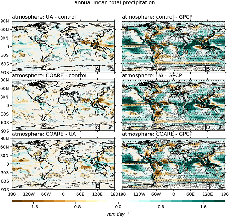
Figure 6. Differences in annual mean precipitation climatology between simulations with different bulk flux algorithms (left column) and annual mean precipitation biases relative to GPCP (right column). Stippling designates regions where the absolute value of the difference is larger than the interannual standard deviation from the E3SMv1 pre-industrial control run.

Regional precipitation changes further poleward consist of a patchwork of small (though significant) precipitation changes, without any obvious pattern. This may be because precipitation changes in these regions occur due to differences in both circulation and moisture source region evaporation, with different processes dominating in different seasons. Seasonal analyses (not shown) support this to some extent. For example, summer precipitation in UA and COARE, relative to control, show a dipole with less precipitation in northwest Europe and more in the Iberian peninsula. Such a dipole has been linked to Atlantic multi-decadal Gulf Stream SST variability (e.g., Palter, 2015) so it is possible that the algorithm-induced Gulf Stream heat flux changes in our study have the same effect as the multidecadal SST variability-induced heat flux changes seen in observations. Meanwhile, in winter, a different and roughly opposite precipitation change occurs — wetter over the United Kingdom and drier in southwest Europe. A similar pattern occurs in the northwest Pacific between Alaska and California. Observational evidence (e.g., Wills et al., 2016; Wills and Thompson, 2018) suggests that these changes could be caused by circulation changes related to Gulf Stream and Kuroshio heat flux changes, but more detailed study is needed to better understand this.

Also shown in Figure 6 are biases relative to the GPCP long-term mean. The biases are generally larger than the differences between simulations, and therefore have very similar patterns for all three atmosphere simulations. While the spatial patterns of biases do not offer a clear differentiation between algorithms, the global mean statistics do. For the global mean bias, COARE has the lowest (+0.32 mm day⁻¹), followed by UA (+0.37 mm day⁻¹) then control (+0.38 mm day⁻¹). For the root mean square error (RMSE), COARE again has the lowest (0.98 mm day⁻¹), while control and UA have very similar values (1.02 mm day⁻¹). These global annual mean figures obscure more nuanced regional and seasonal patterns, making selection of a “best” algorithm even more challenging.

The largest precipitation biases in Figure 6 occur in the tropics, and especially in the warm pool of the Indian and Pacific oceans. This region is examined more closely in Figure 7, which shows distinct patterns of zonal mean bias in different seasons. All seasons share the feature that the model simulations generally have an exaggerated double maximum compared to GPCP. This is a widespread and long-standing problem in Earth system models (e.g., Zhang et al., 2015) and so it is interesting to note that algorithm choice makes some notable differences. In particular, UA has a markedly lower bias north of the equator in boreal summer (JJA) and COARE has the most realistic results in boreal spring (MAM). However, no single algorithm has the best results in all seasons. This point is reinforced by the precipitation RMSE for this sub-region: UA has the lowest in JJA and SON; COARE has the lowest in MAM; control has the lowest in DJF.

FIGURE 7

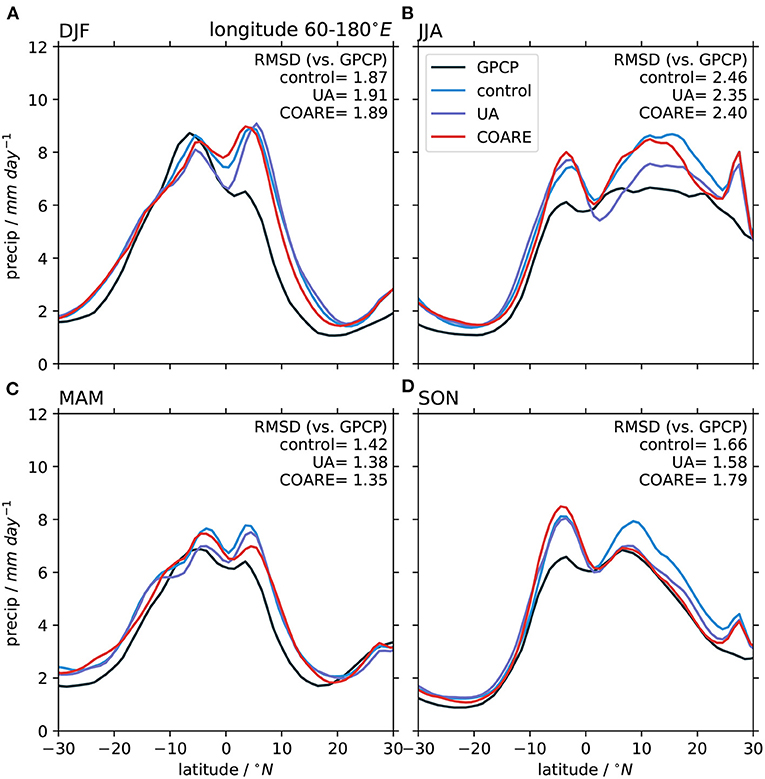
Figure 7. Zonal mean, seasonal mean precipitation from the three atmosphere simulations and GPCP observational data: (A) December to February; (B) June to August; (C) March to May; (D) September to November. The zonal sector considered is 60°E to 180°E. GPCP data were bilinearly interpolated to the same 1° grid as the other data before calculating. Text in each panel shows the area-weighted root mean square difference, in mm day⁻¹, between each model and the GPCP data, calculated from gridded data rather than from the zonal means.

Table 3 shows that, relative to control, both UA and COARE have lower global (land and ocean combined) mean precipitation. This is in line with the evaporation changes shown in Table 2, demonstrating that, at least in a global sense, there is a general balance between evaporation and precipitation changes.

TABLE 3

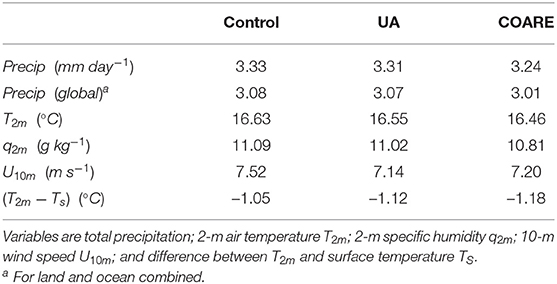
Table 3. Long-term annual mean near-surface meteorology from atmosphere simulations, averaged over global oceans, unless otherwise indicated.

We next look at other aspects of near surface meteorology affected by choice of bulk flux algorithm, bearing in mind that the method of forcing the atmosphere model with specified sea surface temperatures strongly constrains some fields. Mean 2 m air temperature over the oceans is highest in control, followed by UA, with COARE the lowest. The differences at first glance appear modest (< 0.2°C between control and COARE), but when reformulated as a difference between surface and 2 m temperature (also shown in Table 3), they seem somewhat more significant. The same is true of 2 m specific humidity: the absolute values appear similar but, considering that the differences arise just 2 m above surfaces of identical temperature, the size of the differences is more surprising. Finally, and arguably most importantly, the 10 m wind speed is reduced in both UA and COARE compared to control. This result is significant as it suggests that some of the atmosphere simulation flux changes, discussed above, occur due to changes in wind speed rather than changes in stability and roughness formulations.

Other changes in model climate higher in the atmosphere also occur. We briefly mention a few (and refer to relevant figures in the Supplementary Material). Coherent patterns of zonal wind changes occur throughout the full depth of the troposphere (Supplementary Figures 3, 4). These changes bear some resemblance to changes induced by a decrease in surface roughness in Polichtchouk and Shepherd (2016), though in our case the changes are smaller and mostly limited to the winter hemisphere. The global mean temperatures at several different pressure levels (Supplementary Figures 5, 6) are reduced in both UA and COARE, relative to control. We suggest that this is a result of the net heat flux changes, though this interpretation is slightly complicated by net heat flux changes over land, which we do not consider here. Likewise, we suggest that changes in precipitable water (reduced in UA and COARE, relative to control; not shown) are due to reduced ocean evaporation in UA and COARE.

There are also differences in certain metrics that govern model simulations of variability and climate change. Arguably most important is the net top-of-atmosphere (TOA) radiation. Control has the smallest, at +0.58 W m⁻², followed by UA (+1.05 W m⁻²) then COARE (+1.54 W m⁻²). While the absolute values from our relatively short sensitivity tests may not be especially meaningful due to large internannual variability (e.g., Loeb et al., 2018), the differences are important, especially considering the magnitude of biases seen in Golaz et al. (2019) who reported TOA imbalance smaller than observed in both the coupled (model minus observations = −0.54 W m⁻²) and AMIP (model minus observations = −0.71 W m⁻²) simulations. Noting that those simulations used the control algorithm, and based on the differences between the three algorithms, UA therefore does best at correcting this bias, while COARE slightly overshoots. The differences arise from a combination of changes in clouds and clear-sky longwave emission.

High quality satellite observations from CERES-EBAF v4.1 data allow calculation of mean biases and root-mean-square differences (RMSD) for several TOA radiation quantities (Table 4). In most quantities, UA is intermediate between COARE and control. This means that the smallest bias usually occurs with control (e.g., TOA net longwave) or COARE (e.g., TOA net shortwave). This does, however, conceal a number of more complicated regional biases. For example, compared to control, COARE seems to reduce the mean bias in net cloud radiative effect, but part of this improvement comes from COARE's increased bias in subtropical stratocumulus shortwave cloud forcing. Similarly, we see that UA has the smallest net cloud forcing RMSD, despite the fact that COARE has the smallest net cloud forcing mean bias. We also note, in reference to the above discussion of net TOA radiation, that UA has the smallest bias and RMSD in that quantity.

TABLE 4

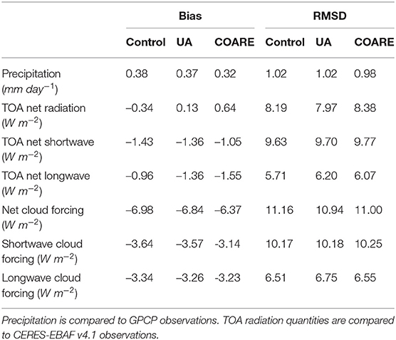
Table 4. Global mean and global root-mean-square (RMS) of annual mean differences between model and observations.

3.3. Ocean Model Sensitivity

Changes in the ocean model are, like changes in the atmosphere model, constrained by the forcing dataset. In fact, for the ocean model the forcing is a stronger constraint because the wind speed—arguably the biggest factor in the atmosphere model changes seen above—is prescribed. Nonetheless, we do see ocean model responses due to the subtle changes in net heat flux, evaporation and wind stress. These are described here.

The SST in the ocean simulations is able to vary, though it is strongly constrained by the air temperature in the forcing. The differences seen in Table 5 are therefore reflecting the different algorithms' preferred (T_2m − T_s) values, shown in Table 3: COARE has the highest (T_s − T_2m) and therefore the highest T_s, followed by UA, then control. While the SST is not able to respond fully to the differences in net heat flux, the ocean heat content (OHC) is able to respond more. We therefore see that changes in OHC (denoted ΔOHC) over the course of the ocean simulations do reflect the differences in net heat flux: the algorithms are ranked control, then UA, then COARE, in increasing order for both SST and ΔOHC. It should be noted that the differences in ΔOHC between model runs are of a comparable magnitude to observed decadal variability and trends, and are therefore physically meaningful.

TABLE 5

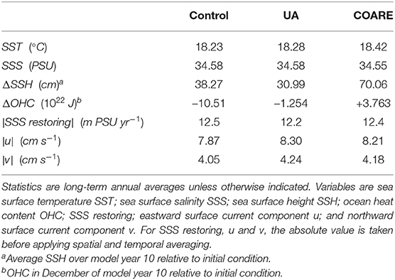
Table 5. Ocean simulation global mean statistics.

Changes in evaporation could, in principle, affect both ocean salinity and sea level. However, surface salinity is subject to salinity restoring (the model field is relaxed to observational climatology; see Petersen et al., 2019 for further details) and this effectively cuts any link between evaporation changes and ocean salinity changes. It is therefore not surprising that all three ocean simulations have very similar surface salinity (Table 5). We can however, look at the magnitude of salinity restoring that is required to stop the model drifting away from observations. The mean absolute values are similar for all three simulations: UA has the lowest value, followed by COARE.

The changes in sea surface height (ΔSSH in Table 5) over the course of each ocean simulation are all of unrealistically large magnitude, likely due to a systematic imbalance between precipitation in the forcing data set and evaporation calculated in the model. However, differences (between ocean simulations) in the sea level change (Table 5) do reflect the evaporation differences seen in Table 2: UA has the largest evaporation and therefore the smallest sea level rise, while COARE has the smallest evaporation and the largest sea level rise. The remainder of the sea surface height changes include thermosteric effects, i.e., the expansion of sea water as it warms. The thermosteric component is isolated by subtracting the global ocean mean change due to evaporation. Thus, the difference between two algorithms can be expressed as:

$\begin{array}{l}\Delta SS{H}_{thermosteric}^{A-B}=(SS{H}_{year10}^A-SS{H}_{initial}^A)\\ -(SS{H}_{year10}^B-SS{H}_{initial}^B)+({\displaystyle \sum _{time}}\left[\overline{E_A}-\overline{E_B}\right])& (4)\end{array}$

where A and B denote the two algorithms being compared, $\overline{E_{A,B}}$ are the global mean evaporation rates and the summation gives the cumulative evaporation difference. The spatial patterns of differences (between different bulk flux algorithms) are shown in Figure 8. Relative to control, UA and COARE result in similar changes, albeit with larger magnitudes for COARE. The changes are fairly symmetric about the equator, with the following key features: small changes of both signs for most regions equatorward of 15°; larger negative changes in the tropical east Pacific; relatively large increases between 15° and 45°; and large decreases poleward of this, especially in the Southern Ocean. This all suggests that much of the extra heat content of the UA and COARE simulations, caused by the larger net heat flux with these algorithms compared to control, ends up being “stored” in the subtropics and midlatitudes.

FIGURE 8

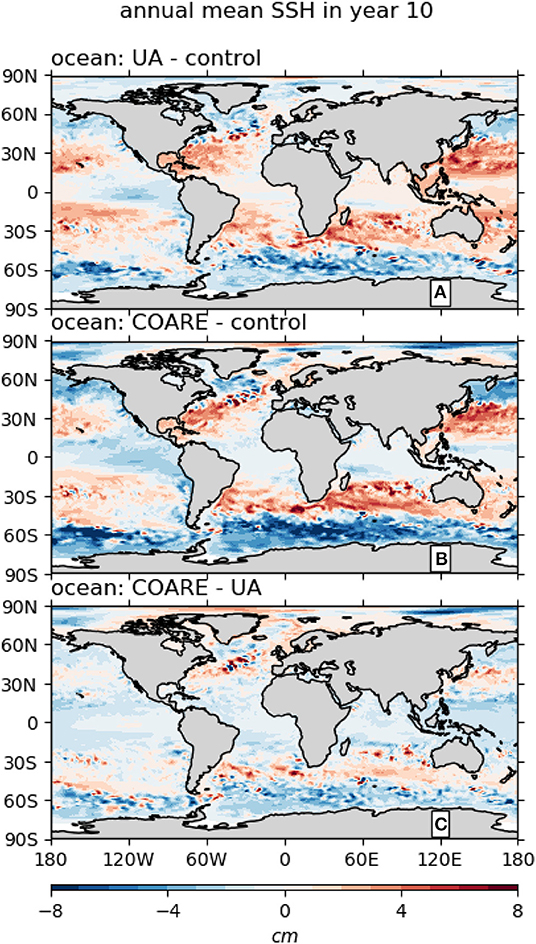
Figure 8. Differences in model year 10 sea surface height between simulations with different ocean surface bulk flux parameterizations. The changes in sea surface height due to evaporation differences have been removed as in Equation (4).

Ocean surface velocity is strongly constrained by the wind field specified in the forcing data. However, differences in velocity component magnitudes do occur (Table 5). We see that UA has the highest velocities, followed closely by COARE, and control has the lowest by a considerable margin. Note that this is the reverse of the pattern seen in the atmosphere 10 metre wind speeds seen in Table 3. Both of these changes are consistent with the fact that, for a particular wind speed, UA gives the largest wind stress, followed by COARE then control. Such differences were also found (at least for moderate wind speeds) in Zeng et al. (1998; their Figure 3C). This means that, where wind speeds are specified (in the ocean simulations) UA gives the largest wind stress and therefore the highest ocean surface velocities. On the other hand, when the wind speed can vary but the surface velocity is fixed (in the atmosphere simulations), UA results in the lowest wind speeds while giving similar wind stress.

A number of other variables are affected by the choice of bulk flux algorithm, though the changes are relatively minor. The Atlantic Meridional Atlantic Circulation (AMOC) is unrealistically weak in all three simulations (as has been noted in other E3SMv1 simulations; Golaz et al., 2019; Petersen et al., 2019) and there are only minor differences between them. However, AMOC is slightly stronger in UA and control than in COARE (Supplementary Figure 7). Possibly related to this are changes in wintertime ocean mixed layer depths in the North Atlantic Deep Water formation regions (not shown) and changes in the global meridional heat transport (MHT; Figure 9). However, global MHT integrates more processes than just the AMOC (e.g., Forget and Ferreira, 2019), and it is in fact the tropical maxima of MHT (shallower circulations more directly linked to surface fluxes) that are changed most—generally of slightly larger magnitude in UA than in control and COARE. As with the AMOC, the MHT differences do not have large enough impacts to significantly reduce the model's background biases. Even so, we suggest that the sensitivity of ocean circulation to algorithm choice deserves longer model runs and further study, beyond the more directly affected quantities discussed here.

FIGURE 9

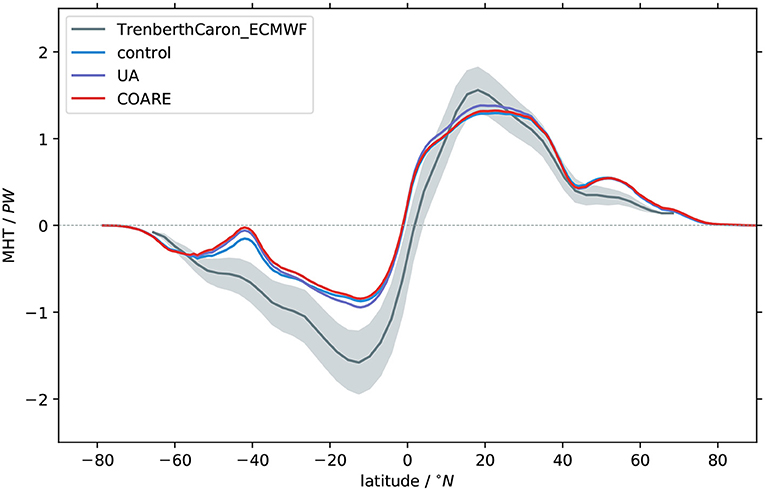
Figure 9. Mean global meridional ocean heat transport (positive northwards) from ocean simulations. Also shown is a reanalysis-based observational estimate from Trenberth and Caron (2001): shading represents ±1 standard error, based on their error analysis using assumed uncertainties in derived surface fluxes.

4. Conclusions and Further Discussion

We have performed sensitivity tests of three ocean surface flux parameterizations in the atmosphere and ocean components of E3SM. Spatial patterns of heat flux and wind stress sensitivity differ significantly between ocean and atmosphere simulations, with larger magnitudes of changes in the atmosphere simulations. This is not surprising given that wind speed—which strongly affects surface fluxes—can vary in the atmosphere simulations but is specified by the forcing data in ocean simulations. What is perhaps more surprising is the degree of consistency (between ocean and atmosphere simulations) of the global mean latent heat flux and net surface heat flux sensitivity.

The impact of wind speed-flux feedbacks on the atmosphere simulation sensitivity highlights the central role of wind speed in determining fluxes. Thus, the ocean simulations (with fixed wind speeds) tell us more about the theoretical aspects of algorithm design (e.g., the functional forms of stability and roughness formulae) while at the same time revealing how the ocean may respond to flux changes. On the other hand, the atmosphere simulations (where wind speed can vary) tell us about the combined effects of theoretical changes and resultant wind speed differences. Thus, our results show that, relative to the control algorithm, COARE has greater theoretical differences, but when wind speeds are allowed to vary, UA has a greater overall effect. A regional example of this is shown in Figure 10 for the Gulf Stream, where both COARE and UA have lower magnitude of annual mean latent heat flux than control (Figure 1). Figure 10 shows that, for wind speeds greater than about 12 m s⁻¹, both COARE and UA have lower magnitude latent heat fluxes than control. However, it is also clear that the distribution of wind speeds are shifted, with UA having the lowest speeds, followed by COARE and then control having the highest. Another illustration of the importance of wind speed changes in the atmosphere simulations is the degree of correspondence between the latent heat flux changes (Figure 1, left column) and the wind speed changes (Figure 2, left column): patterns of negative wind speed differences match closely with positive latent heat flux differences (i.e., due to the sign convention, negative flux magnitude differences).

FIGURE 10

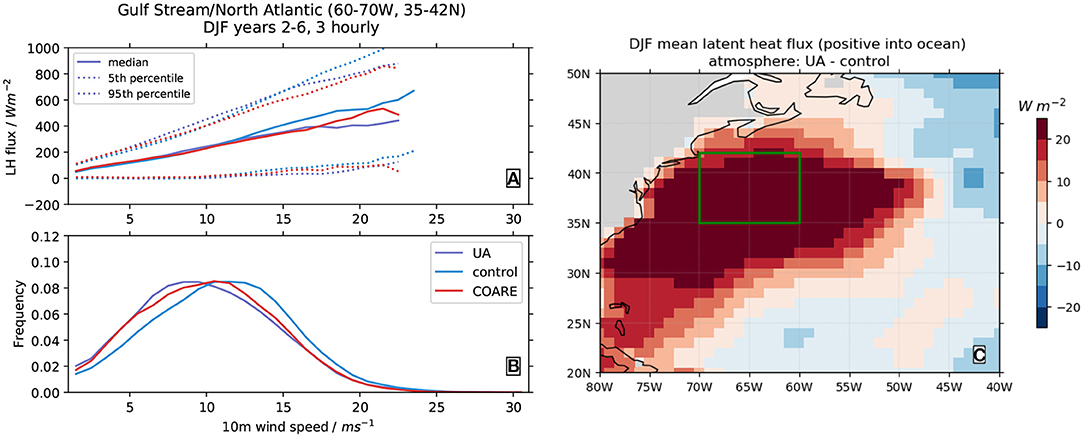
Figure 10. (A) Latent heat flux quantiles, as functions of 10-m wind speed, and (B) 10-m wind speed distributions, for the three atmosphere simulations in a region around the Gulf Stream (60−70°W, 35−42°N). The quantiles and wind speed distribution are calculated from 3-hourly model output from the winter season (December, January, and February) over model years 2−6 of each simulation, binned into 1 m s⁻¹ bins. (C) December to February multi-year mean latent heat flux difference between UA and control atmosphere simulations, with the region used in (A,B) shown by the green box. Note that the heat flux sign convention in (A) is opposite to that used in (C): positive values correspond to evaporation. The colors shown in the legend of (B) also apply to (A).

An important caveat to this interpretation, however, is that some of the impacts of the UA algorithm are tempered by its use of temperature-dependent L_v (latent heat of vaporization). Thus, although UA has larger differences (relative to control) in latent heat flux and net heat flux, COARE has a larger difference in evaporation, and therefore a larger impact on precipitation. This can have other important consequences for modeled global energy and water cycles, as was seen in the ocean simulations: compared to control, UA simulates a sea level fall and OHC increase, while COARE simulates sea level rise and OHC increase. Of course, the comparison with control is somewhat arbitrary and does not have any physical significance when interpreting any single model simulation. It does however, underscore that the algorithms give different portrayals of the links between global energy and water cycles. This point is particularly important for coupled Earth system modeling, where conservation of water and energy are important constraints in model realism. The effects of flux algorithm choice in this respect are the subject of ongoing coupled model development and testing within the E3SM project.

It is worth noting that the absolute values (from any single simulation) of quantities like ΔOHC are not physically meaningful. Instead, they are a product of the disequilibrium between the forcing data and initial conditions [see Strobach et al. (2018) for a thorough exploration of such disequilibrium conditions]. Nonetheless, the differences between algorithms in their responses to this disequilibrium are meaningful: these kind of differences are exactly what may yield variations in estimates of transient climate response to greenhouse gas and other anthropogenic climate forcing.

We finish by revisiting our aims for this study and summarizing the key results for each:

1. Our atmosphere sensitivity tests suggest that parts of the tropical Indo-Pacific region (~20°N−20°S, 60°E−150°W), along with western boundary currents, are hotspots of algorithm differences, as might be expected from the fact that these regions are the continued focus of ocean-atmosphere interaction research (e.g., Edson et al., 2013). In addition, our ocean sensitivity tests highlight the tropical east Pacific and the Southern Ocean as regions of uncertainty, worthy of further study. It is interesting to note that these regions include a number of “edge cases” recognized in recent ocean-atmosphere interaction research. The Indo-Pacific warm pool can exhibit strong diurnal SST warming (Fairall et al., 1996a) and gusty winds in thunderstorm cold pools (Zeng et al., 2002). Western boundary currents and the eastern tropical Pacific are both domains of strong gradients with complex wind-wave-current interactions which are not well-understood (Villas Bôas et al., 2019). The Southern Ocean features consistently strong winds and extreme wave conditions. These cases lead to uncertainties in fluxes and differences between the algorithms, both by design and due to insufficient direct flux observations to constrain bulk algorithm formulation.

2. We find that the choice of test methodology seems to highlight different aspects of the algorithms' differences. Atmosphere simulations, by allowing a wind speed-flux feedback cycle, show the highest absolute magnitudes of flux differences between algorithms. This has the advantage of allowing investigation of changes in wind speed distribution due to differences in algorithms' surface roughness formulations. However, it has disadvantages in that changes in any particular location may be influenced by remotely forced atmospheric circulation changes (e.g., tropical forcing of midlatitude circulation), and that changes may be due to model internal variability (i.e., chaotic differences in weather patterns). Our significance testing is intended to address this, but the relatively short simulations used here are certainly a minor limitation of this study.

3. Finally, we have demonstrated that impacts of algorithm choice are seen throughout the atmosphere and ocean models. Of particular importance in the atmosphere simulations are the systematic circulation changes and differences in global mean precipitation and TOA radiative effects. There are also important regional changes — for example in heat fluxes in the seas adjacent to the Asian Monsoon system, with associated precipitation changes over land. In the ocean, we see small but notable impacts on meridional overturning circulations and meridional heat transport. It is interesting to speculate that the changes seen in these quantities in a coupled model setup (where the larger magnitude flux changes seen in the atmosphere simulations might be imposed on the ocean) could be larger than seen in our ocean simulation results. This possibility, along with the differences in global energy and water cycle responses discussed above, are good reasons to pursue coupled Earth system model sensitivity testing in future studies. Indeed, such efforts are already underway in the E3SM project.

In the absence of a definitive observational basis to rank algorithms by flux biases, these other changes offer a way to inform algorithm choice. In particular, both UA and COARE improve on the control algorithm in global mean precipitation and TOA radiative metrics, though there are some important regional changes that should also be considered. In the ocean, UA seems to reduce biases slightly (in comparison to control) in the Atlantic meridional overturning circulation and meridional heat transport.

Data Availability Statement

1. Model source code is available at https://github.com/E3SM-Project/E3SM/commit/121d1c99d1c8573dc9e57536a0819ec7f423e2ee. Raw model output is available at https://portal.nersc.gov/archive/home/j/jeyre/www/. Intermediate data used to create the figures and tables in this article are available at https://osf.io/4enh5/. Computer code used to create the figures and tables is available at https://bitbucket.org/jack_eyre/oceanfluxes_13apr2021. Some additional calculations were used from the MPAS-Analysis package (https://github.com/MPAS-Dev/MPAS-Analysis).

2. OAflux, CERES-EBAF and GPCP are publicly available from repositories given in the References section and cited in the text.

Author Contributions

JRE implemented the UA algorithm in E3SM, performed the model runs and data analysis, and led the writing. XZ provided guidance on modeling strategy and analysis methods, and contributed to the writing. KZ implemented the COARE algorithm in E3SM and contributed to the writing. All authors contributed to the article and approved the submitted version.

Funding

This research was supported by the U.S. Department of Energy (DE-SC0016533, DE-AC52-07NA27344/B639244). KZ was supported by the Office of Science of the U.S. Department of Energy as part of the Earth System Modeling Program. The Pacific Northwest National Laboratory is operated for DOE by Battelle Memorial Institute under contract DE-AC05-76RL01830.

Conflict of Interest

At time of article submission, JRE is a member of the research group of one of the topic editors for this Research Topic (Dr. Meghan F. Cronin).

The remaining authors declare that the research was conducted in the absence of any commercial or financial relationships that could be construed as a potential conflict of interest.

Acknowledgments

We thank Thomas Tonazzio and Chris Fairall for providing the COARE algorithm code. We thank Luke Van Roekel and Po-Lun Ma for assistance in setting up the model runs. Michael Brunke, Joellen Russell, and Chris Castro provided much useful advice about details of the flux algorithms and interpretation of results. We thank the editor and reviewers for their constructive comments. This research used resources of the National Energy Research Scientific Computing Center (NERSC), a U.S. Department of Energy Office of Science User Facility operated under Contract No. DE-AC02-05CH11231. We gratefully acknowledge the computing resources provided on Blues, a high-performance computing cluster operated by the Laboratory Computing Resource Center at Argonne National Laboratory.

Supplementary Material

The Supplementary Material for this article can be found online at: https://www.frontiersin.org/articles/10.3389/fmars.2021.642804/full#supplementary-material

References

Adler, R. F., Huffman, G. J., Chang, A., Ferraro, R., Xie, P.-P., Janowiak, J., et al. (2003). The version-2 global precipitation climatology project (GPCP) monthly precipitation analysis (1979–present). J. Hydrometeorol. 4, 1147–1167. doi: 10.1175/1525-7541(2003)004<1147:TVGPCP>2.0.CO;2

CrossRef Full Text | Google Scholar

Adler, R. F., Huffman, G. J., Chang, A., Ferraro, R., Xie, P.-P., Janowiak, J., et al. (2018). GPCP Version 2.3 Combined Precipitation Data Set (Updated Monthly). Available online at: https://psl.noaa.gov/data/gridded/data.gpcp.html (accessed February 07, 2020).

Google Scholar

Beljaars, A. C. M., and Holtslag, A. A. M. (1991). Flux parameterization over land surfaces for atmospheric models. J. Appl. Meteorol. Climatol. 30, 327–341. doi: 10.1175/1520-0450(1991)030<0327:FPOLSF>2.0.CO;2

CrossRef Full Text | Google Scholar

Brodeau, L., Barnier, B., Gulev, S. K., and Woods, C. (2016). Climatologically significant effects of some approximations in the bulk parameterizations of turbulent air–sea fluxes. J. Phys. Oceanogr. 47, 5–28. doi: 10.1175/JPO-D-16-0169.1

CrossRef Full Text | Google Scholar

Brunke, M. A., Fairall, C. W., Zeng, X., Eymard, L., and Curry, J. A. (2003). Which bulk aerodynamic algorithms are least problematic in computing ocean surface turbulent fluxes? J. Clim. 16, 619–635. doi: 10.1175/1520-0442(2003)016<0619:WBAAAL>2.0.CO;2

CrossRef Full Text | Google Scholar

Brunke, M. A., Wang, Z., Zeng, X., Bosilovich, M., and Shie, C.-L. (2011). An assessment of the uncertainties in ocean surface turbulent fluxes in 11 reanalysis, satellite-derived, and combined global datasets. J. Clim. 24, 5469–5493. doi: 10.1175/2011jcli4223.1

CrossRef Full Text | Google Scholar

Brunke, M. A., Zeng, X., and Anderson, S. (2002). Uncertainties in sea surface turbulent flux algorithms and data sets. J. Geophys. Res. Oceans 107, 5–1–5–21. doi: 10.1029/2001JC000992

CrossRef Full Text | Google Scholar

Brunke, M. A., Zeng, X., Misra, V., and Beljaars, A. (2008). Integration of a prognostic sea surface skin temperature scheme into weather and climate models. J. Geophys. Res. 113. doi: 10.1029/2008jd010607

CrossRef Full Text | Google Scholar

Brutsaert, W. (1982). Evaporation into the Atmosphere: Theory, History and Applications. Environmental Fluid Mechanics. Dordrecht: Springer.

Google Scholar

Doelling, D. (2019). CERES Energy Balanced and Filled (EBAF) TOA Monthly Means Data in netCDF Edition4.1. Available online at: 10.5067/TERRA-AQUA/CERES/EBAF-TOA_L3B004.1 (accessed 23, June 2020).

Dyer, A. J. (1974). A review of flux-profile relationships. Bound. Layer Meteorol. 7, 363–372. doi: 10.1007/BF00240838

CrossRef Full Text | Google Scholar

Edson, J. B., Hinton, A. A., Prada, K. E., Hare, J. E., and Fairall, C. W. (1998). Direct covariance flux estimates from mobile platforms at sea*. J. Atmos. Ocean. Technol. 15, 547–562. doi: 10.1175/1520-0426(1998)015<0547:DCFEFM>2.0.CO;2

CrossRef Full Text | Google Scholar

Edson, J. B., Jampana, V., Weller, R. A., Bigorre, S. P., Plueddemann, A. J., Fairall, C. W., et al. (2013). On the exchange of momentum over the open ocean. J. Phys. Oceanogr. 43, 1589–1610. doi: 10.1175/JPO-D-12-0173.1

CrossRef Full Text | Google Scholar

Fairall, C. W., Bradley, E. F., Godfrey, J. S., Wick, G. A., Edson, J. B., and Young, G. S. (1996a). Cool-skin and warm-layer effects on sea surface temperature. J. Geophys. Res. Oceans 101, 1295–1308. doi: 10.1029/95JC03190

CrossRef Full Text | Google Scholar

Fairall, C. W., Bradley, E. F., Hare, J. E., Grachev, A. A., and Edson, J. B. (2003). Bulk parameterization of air–sea fluxes: updates and verification for the COARE Algorithm. J. Clim. 16, 571–591. doi: 10.1175/1520-0442(2003)016<0571:BPOASF>2.0.CO;2

CrossRef Full Text | Google Scholar

Fairall, C. W., Bradley, E. F., Rogers, D. P., Edson, J. B., and Young, G. S. (1996b). Bulk parameterization of air-sea fluxes for tropical ocean-Global atmosphere coupled-Ocean atmosphere response experiment. J. Geophys. Res. Oceans 101, 3747–3764. doi: 10.1029/95JC03205

CrossRef Full Text | Google Scholar

Forget, G., and Ferreira, D. (2019). Global ocean heat transport dominated by heat export from the tropical Pacific. Nat. Geosci. 12, 351–354. doi: 10.1038/s41561-019-0333-7

CrossRef Full Text | Google Scholar

Găinuşă-Bogdan, A., Braconnot, P., and Servonnat, J. (2015). Using an ensemble data set of turbulent air-sea fluxes to evaluate the IPSL climate model in tropical regions. J. Geophys. Res. Atmos. 120, 4483–4505. doi: 10.1002/2014JD022985

CrossRef Full Text | Google Scholar

Golaz, J.-C., Caldwell, P. M., Roekel, L. P. V., Petersen, M. R., Tang, Q., Wolfe, J. D., et al. (2019). The DOE E3SM coupled model version 1: overview and evaluation at standard resolution. J. Adv. Model. Earth Syst. 11, 2089–2129. doi: 10.1029/2018MS001603

CrossRef Full Text | Google Scholar

Harrop, B. E., Ma, P.-L., Rasch, P. J., Neale, R. B., and Hannay, C. (2018). The role of convective gustiness in reducing seasonal precipitation biases in the Tropical West Pacific. J. Adv. Model. Earth Syst. 10, 961–970. doi: 10.1002/2017MS001157

CrossRef Full Text | Google Scholar

Harrop, B. E., Ma, P.-L., Rasch, P. J., Qian, Y., Lin, G., and Hannay, C. (2019). Understanding monsoonal water cycle changes in a warmer climate in E3SMv1 using a normalized gross moist stability framework. J. Geophys. Res. Atmos. 124, 10826–10843. doi: 10.1029/2019JD031443

CrossRef Full Text | Google Scholar

Holdsworth, A. M., and Myers, P. G. (2015). The influence of high-frequency atmospheric forcing on the circulation and deep convection of the Labrador Sea. J. Clim. 28, 4980–4996. doi: 10.1175/JCLI-D-14-00564.1

CrossRef Full Text | Google Scholar

Holtslag, A. A. M., Bruijn, E. I. F. D., and Pan, H.-L. (1990). A high resolution air mass transformation model for short-range weather forecasting. Mon. Weather Rev. 118, 1561–1575. doi: 10.1175/1520-0493(1990)118<1561:AHRAMT>2.0.CO;2

CrossRef Full Text | Google Scholar

Hu, Q., Jiang, D., Lang, X., and Yao, S. (2021). Moisture sources of summer precipitation over eastern China during 1979–2009: a Lagrangian transient simulation. Int. J. Climatol. 41, 1162–1178. doi: 10.1002/joc.6781

CrossRef Full Text | Google Scholar

Kader, B. A., and Yaglom, A. M. (1990). Mean fields and fluctuation moments in unstably stratified turbulent boundary layers. J. Fluid Mech. 212, 637–662. doi: 10.1017/S0022112090002129

CrossRef Full Text | Google Scholar

Kostov, Y., Johnson, H. L., and Marshall, D. P. (2019). AMOC sensitivity to surface buoyancy fluxes: the role of air-sea feedback mechanisms. Clim. Dyn. 53, 4521–4537. doi: 10.1007/s00382-019-04802-4

CrossRef Full Text | Google Scholar

Large, W. G., and Caron, J. M. (2015). Diurnal cycling of sea surface temperature, salinity, and current in the CESM coupled climate model. J. Geophys. Res. Oceans 120, 3711–3729. doi: 10.1002/2014JC010691

CrossRef Full Text | Google Scholar

Large, W. G., and Pond, S. (1981). Open ocean momentum flux measurements in moderate to strong winds. J. Phys. Oceanogr. 11, 324–336.

Google Scholar

Large, W. G., and Pond, S. (1982). Sensible and latent heat flux measurements over the ocean. J. Phys. Oceanogr. 12, 464–482.

Google Scholar

Large, W. G., and Yeager, S. G. (2004). Diurnal to Decadal Global Forcing for Ocean and Sea-Ice Models: The Data Sets and Flux Climatologies. NCAR Tech. Note NCAR/TN-460+STR, University Corporation for Atmospheric Research.

Google Scholar

Large, W. G., and Yeager, S. G. (2009). The global climatology of an interannually varying air-sea flux data set. Clim. Dyn. 33, 341–364. doi: 10.1007/s00382-008-0441-3

CrossRef Full Text | Google Scholar

L'Ecuyer, T. S., Beaudoing, H. K., Rodell, M., Olson, W., Lin, B., Kato, S., et al. (2015). The observed state of the energy budget in the early twenty-first century. J. Clim. 28, 8319–8346. doi: 10.1175/JCLI-D-14-00556.1

CrossRef Full Text | Google Scholar

Lélé, M. I., Leslie, L. M., and Lamb, P. J. (2015). Analysis of low-level atmospheric moisture transport associated with the West African Monsoon. J. Clim. 28, 4414–4430. doi: 10.1175/JCLI-D-14-00746.1

CrossRef Full Text | Google Scholar

Li, C., von Storch, J.-S., and Marotzke, J. (2013). Deep-ocean heat uptake and equilibrium climate response. Clim. Dyn. 40, 1071–1086. doi: 10.1007/s00382-012-1350-z

CrossRef Full Text | Google Scholar

Liu, W., Cook, K. H., and Vizy, E. K. (2020). Role of the West African westerly jet in the seasonal and diurnal cycles of precipitation over West Africa. Clim. Dyn. 54, 843–861. doi: 10.1007/s00382-019-05035-1

CrossRef Full Text | Google Scholar

Loeb, N. G., Doelling, D. R., Wang, H., Su, W., Nguyen, C., Corbett, J. G., et al. (2018). Clouds and the Earth's radiant energy system (CERES) energy balanced and filled (EBAF) top-of-atmosphere (TOA) Edition-4.0 data product. J. Clim. 31, 895–918. doi: 10.1175/JCLI-D-17-0208.1

CrossRef Full Text | Google Scholar

Palter, J. B. (2015). The role of the Gulf stream in European climate. Annu. Rev. Mar. Sci. 7, 113–137. doi: 10.1146/annurev-marine-010814-015656

PubMed Abstract | CrossRef Full Text | Google Scholar

Pathak, A., Ghosh, S., Martinez, J. A., Dominguez, F., and Kumar, P. (2017). Role of oceanic and land moisture sources and transport in the seasonal and interannual variability of summer monsoon in India. J. Clim. 30, 1839–1859. doi: 10.1175/JCLI-D-16-0156.1

CrossRef Full Text | Google Scholar

Petersen, M. R., Asay-Davis, X. S., Berres, A. S., Chen, Q., Feige, N., Hoffman, M. J., et al. (2019). An evaluation of the ocean and sea ice climate of E3SM using MPAS and interannual CORE-II forcing. J. Adv. Model. Earth Syst. 11, 1438–1458. doi: 10.1029/2018MS001373

CrossRef Full Text | Google Scholar

Polichtchouk, I., and Shepherd, T. G. (2016). Zonal-mean circulation response to reduced air–sea momentum roughness. Q. J. R. Meteorol. Soc. 142, 2611–2622. doi: 10.1002/qj.2850

CrossRef Full Text | Google Scholar

Rhein, M., Rintoul, S., Aoki, S., Campos, E., Chambers, D., Feely, R., et al. (2013). “Observations: ocean,” in Climate Change 2013: The Physical Science Basis. Contribution of Working Group I to the Fifth Assessment Report of the Intergovernmental Panel on Climate Change, eds T. Stocker, D. Qin, G.-K. Plattner, M. Tignor, S. Allen, J. Boschung, A. Nauels, Y. Xia, V. Bex, and P. Midgley (Cambridge; New York, NY: Cambridge University Press), 255–316.

Google Scholar

Smith, S. D. (1988). Coefficients for sea surface wind stress, heat flux, and wind profiles as a function of wind speed and temperature. J. Geophys. Res. Oceans 93, 15467–15472.

Google Scholar

Strobach, E., Molod, A., Forget, G., Campin, J.-M., Hill, C., Menemenlis, D., et al. (2018). Consequences of different air-sea feedbacks on ocean using MITgcm and MERRA-2 forcing: implications for coupled data assimilation systems. Ocean Model. 132, 91–111. doi: 10.1016/j.ocemod.2018.10.006

CrossRef Full Text | Google Scholar

Trenberth, K. E., and Caron, J. M. (2001). Estimates of meridional atmosphere and ocean heat transports. J. Clim. 14, 3433–3443. doi: 10.1175/1520-0442(2001)014<3433:EOMAAO>2.0.CO;2

CrossRef Full Text | Google Scholar

Tsujino, H., Urakawa, S., Nakano, H., Small, R. J., Kim, W. M., Yeager, S. G., et al. (2018). JRA-55 based surface dataset for driving ocean–sea-ice models (JRA55-do). Ocean Model. 130, 79–139. doi: 10.1016/j.ocemod.2018.07.002

CrossRef Full Text | Google Scholar

Villas Bôas, A. B., Ardhuin, F., Ayet, A., Bourassa, M. A., Brandt, P., Chapron, B., et al. (2019). Integrated observations of global surface winds, currents, and waves: requirements and challenges for the next decade. Front. Mar. Sci. 6:425. doi: 10.3389/fmars.2019.00425

CrossRef Full Text

Wills, S. M., and Thompson, D. W. J. (2018). On the observed relationships between wintertime variability in Kuroshio–Oyashio extension sea surface temperatures and the atmospheric circulation over the North Pacific. J. Clim. 31, 4669–4681. doi: 10.1175/JCLI-D-17-0343.1

CrossRef Full Text | Google Scholar

Wills, S. M., Thompson, D. W. J., and Ciasto, L. M. (2016). On the observed relationships between variability in Gulf stream sea surface temperatures and the atmospheric circulation over the North Atlantic. J. Clim. 29, 3719–3730. doi: 10.1175/JCLI-D-15-0820.1

CrossRef Full Text | Google Scholar

Yu, L. (2019). Global air–sea fluxes of heat, fresh water, and momentum: energy budget closure and unanswered questions. Annu. Rev. Mar. Sci. 11, 227–248. doi: 10.1146/annurev-marine-010816-060704

PubMed Abstract | CrossRef Full Text | Google Scholar

Yu, L., Jin, X., and Weller, R. A. (2006). Objectively Analyzed Air-Sea Fluxes (OAFlux) For Global Oceans. Available online at: ftp://ftp.whoi.edu/pub/science/oaflux/data_v3/monthly/evaporation/ (accessed March 28, 2020).

Yu, L., and Weller, R. A. (2007). Objectively analyzed air–sea heat fluxes for the global ice-free oceans (1981–2005). Bull. Am. Meteorol. Soc. 88, 527–540. doi: 10.1175/BAMS-88-4-527

CrossRef Full Text | Google Scholar

Zender, C. (2020). netCDF Operator (NCO) User Guide. Technical report. Available online at: http://nco.sf.net/nco.pdf.

Zeng, X., and Beljaars, A. (2005). A prognostic scheme of sea surface skin temperature for modeling and data assimilation. Geophys. Res. Lett. 32:L14605. doi: 10.1029/2005GL023030

CrossRef Full Text | Google Scholar

Zeng, X., Zhang, Q., Johnson, D., and Tao, W.-K. (2002). Parameterization of wind gustiness for the computation of ocean surface fluxes at different spatial scales. Mon. Weather Rev. 130, 2125–2133. doi: 10.1175/1520-0493(2002)130<2125:POWGFT>2.0.CO;2

CrossRef Full Text | Google Scholar

Zeng, X., Zhao, M., and Dickinson, R. E. (1998). Intercomparison of bulk aerodynamic algorithms for the computation of sea surface fluxes using TOGA COARE and TAO data. J. Clim. 11, 2628–2644.

Google Scholar

Zhang, X., Liu, H., and Zhang, M. (2015). Double ITCZ in coupled ocean-atmosphere models: from CMIP3 to CMIP5. Geophys. Res. Lett. 42:2015GL065973. doi: 10.1002/2015GL065973

CrossRef Full Text | Google Scholar