 Benjamin Jacob
 Emil V. Stanev
- Institute of Coastal Systems - Analysis and Modeling, Helmholtz-Zentrum Hereon, Geesthacht, Germany
The hydrodynamic response to morphodynamic variability in the coastal areas of the German Bight was analyzed via numerical experiments using time-referenced bathymetric data for the period 1982–2012. Time-slice experiments were conducted for each year with the Semi-implicit Cross-scale Hydroscience Integrated System Model (SCHISM). This unstructured-grid model resolves small-scale bathymetric features in the coastal zone, which are well-resolved in the high-resolution time-referenced bathymetric data (50 m resolution). Their analysis reveals the continuous migration of tidal channels, as well as rather complex change of the depths of tidal flats in different periods. The almost linear relationship between the cross-sectional inlet areas and the tidal prisms of the intertidal basins in the East Frisian Wadden Sea demonstrates that these bathymetric data describe a consistent morphodynamic evolutionary trend. The numerical experiment results are streamlined to explain the hydrodynamic evolution from 1982 to 2012. Although the bathymetric changes were mostly located in a relatively small part of the model area, they resulted in substantial changes in the M2 tidal amplitudes, i.e., larger than 5 cm in some areas. The hydrodynamic response to bathymetric changes largely exceeded the response to sea level rise. The tidal asymmetry estimated from the model appeared very sensitive to bathymetric evolution, particularly between the southern tip of Sylt Island and the Eider Estuary along the eastern coast. The peak current asymmetry weakened from 1982 to 1995 and even reversed within some tidal basins to become flood-dominant. This would suggest that the flushing trend in the 1980s was reduced or reversed in the second half of the studied period. Salinity also appeared sensitive to bathymetric changes; the deviations in the individual years reached ~22 psu in the tidal channels and tidal flats. One practical conclusion from the present numerical simulations is that wherever possible, the numerical modeling of near-coastal zones must employ time-referenced bathymetry data. The second, perhaps even more important conclusion, is that the progress of morphodynamic modeling in realistic ocean settings with multiple scales and varying bottom forms is strongly dependent on the availability of bathymetric data with appropriate temporal and spatial resolution.
1. Introduction
The spatial and temporal asymmetries in the hydrodynamic energy (Friedrichs, 2011) due to tides and wind waves contribute to landward and seaward sediment transport. The transport direction depends on differences in the magnitude and duration between the ebb and flood tidal currents (Dronkers, 1986). These ebb-flood differences (“tidal asymmetry”) are produced by the distortion of the tidal wave propagating on the shelf and in the estuaries. This is the case in the Wadden Sea (Stanev et al., 2006), as in similar coastal areas (Robins and Davies, 2010). As shown in these studies, switches from ebb-dominant to flood-dominant transport are sensitive to the local water depth, which can change because of sea level rise (SLR), changes in the magnitude of wind waves, and river runoff. Deposition and erosion of sediment results in continuous bathymetry changes, minimizing the spatial asymmetries in the hydrodynamic energy. Bed evolution is explained by a large number of coupled adjustment processes under three types of dynamics: hydrodynamics (currents and waves), sediment dynamics and morphodynamics (de Swart and Zimmerman, 2009; Wang et al., 2012). Human interventions, such as the construction of dikes, dredging and land nourishment, also play an important role in guiding the development of the coastal bathymetry (Flemming, 2002).
Observations and numerical modeling in the coastal zone and in particular in estuaries provide strong evidence for changing bathymetry with largely varying temporal and spatial scales. To the best of the authors' knowledge, most morphodynamic studies have addressed small areas. However, the morphodynamic evolution is not only a limited area problem. It is associated with large-scale atmospheric forcing and tidal oscillations, and the latter are also global. The two-way interaction between coastal ocean water and the open ocean (see, for the upscaling hydrodynamic problem, Schulz-Stellenfleth and Stanev, 2016) needs to be studied in the context of morphodynamic modeling.
Most of coastal, regional, and larger-scale circulation models use fixed bathymetries, although it is known that bathymetry is not static. Therefore, the main motivations in the present study are to (1) describe the morphodynamic evolution of coastal systems at large scales using time-referenced bathymetric observations, (2) compare the magnitudes of hydrodynamic responses to SLR to those caused by the morphodynamic evolution, and (3) address an area larger than an intertidal basin or tidal delta and describe the differences between the hydrodynamics under different and realistic bathymetries. One such area where bathymetry changes have been well sampled in recent decades, is the German Bight.
The German Bight located in the southeastern North Sea (Figure 1) has a maximum depth of ~50 m. A world-renowned intertidal area known as the Wadden Sea composes the coastal zone of this region and stretches along the coastline of the Netherlands, Germany and Denmark. Most of the Wadden Sea is a mesotidal environment (with a tidal range of ~2–4 m), which allows the formation of barrier islands. The area shown in Figure 1 features two major tidal basin systems, the East Frisian Wadden Sea (EFWS) along the southern coast and the North Frisian Wadden Sea (NFWS) along the eastern coast. In the EFWS, multiple deep tidal channels separate individual barrier islands connecting the tidal flats to the open ocean. The southeastern zone is a macrotidal area (with a tidal range exceeding 4 m) with various bathymetric features of different scales, including a number of shoals separated by tidal channels. This part of the Wadden Sea includes the estuaries of the Weser and Elbe Rivers, which are among the major sources of freshwater emptying into the North Sea. Another important estuary, the Ems River, is situated in the western part of the EFWS.
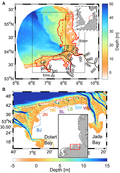
Figure 1. (A) Mean bathymetry for the period from 1982 to 2012 in the German Bight. The inset shows the position of the German Bight in the North Sea. The thick red line delineates the area where time-referenced bathymetry is available. The space between the red dashed and full lines identifies the area where the time intervals between individual samplings is longer than 2 years on average. Numbers show the distance in kilometers along different rivers and their estuaries. Black boxes denote areas of interest shown in later analyses. (B) Magnified view of the area of the EFWS. Individual basins are separated by colored dashed lines and labeled after the names of the barrier islands behind which they are situated: BJ, Borkum Juist; JN, Juist Norderney; NB, Norderney Baltrum; BL, Baltrum Langeoog; LS, Langeoog Spiekeroog; SW, Spiekeroog Wangerooge; WM, Wangerooge Minsener Oog. The black crosses indicate the locations of tide gauge stations in the region. The red box shows the position of the magnified area. The brown dashed line to the north of the barrier islands identifies the open ocean area (to the north of this line), which is subject to a separate analysis.
In the region of this study, tidal asymmetries are caused by the nonlinear deformation of tidal waves in the transition area between the interior German Bight and the shallow Wadden Sea (Stanev et al., 2014). The nonlinear relationship between the transport through inlets and the sea level within the basins of the EFWS (hypsometric control) results in the generation of higher harmonics, creating differences between the flood and ebb tidal flows therein (Maas, 1997; Stanev et al., 2003). Furthermore, gravitational overturning in estuaries creates a pronounced difference between the asymmetries of tidal currents at the bottom and at the surface (Stanev et al., 2015), emphasizing the effect of baroclinicity and its potential impacts on the sediment and morphodynamic balances in the Wadden Sea. In particular, within the southern North Sea, the role of the bed shear stress due to tidal currents in some areas is as important in shaping suspended sediment dynamics as that of the bed shear stress due to wind waves in shaping suspended sediment dynamics (Stanev et al., 2009). These are the shallow areas (e.g., Wadden Sea) where the level of wave-induced turbulence is low as wave heights are limited by the small water depths.
The influence of the water-level elevation and tidal range on sedimentation in the Wadden Sea is explained by Dieckmann et al. (1987). He demonstrated that the area prone to sedimentation displaces with the change of the tidal range, and that this process is controlled by the hypsometry. Long-term bathymetric data for the German Bight (Aufmod, Aufbau von integrierten Modellsystemen zur Analyse der langfristigen Morphodynamik in der Deutschen Bucht Schrottke and Heyer, 2013; Milbradt et al., 2015) document the morphological evolution of the Wadden Sea over a period spanning more than 30 years. The majority of morphological activity (with the largest range of the bed elevation) is observed in the deep channels of the outer estuaries, namely, the EFWS and North Frisian Wadden Sea (NFWS).
Changes in bathymetry exceeding 10 m reveal an active migration of underwater channels. The outer Elbe shows the highest morphological variability. The tidal currents and, in case of the West coast (NFWS), the wind waves are considered the major morphological drivers of these changes (Winter, 2011).
The sediment budget analysis performed by Benninghoff and Winter (2019) for the period between 1998 and 2016 showed that the tidal flats in this region accumulate sediments at a rate higher than the observed mean rate of SLR, which ranges from 2.2 to 6.6 mm/yr for the German Bight (Wahl et al., 2013). Indeed, the SLR scenario of Wachler et al. (2020) demonstrated that elevated tidal flats and deepened tidal channels tend to counteract the pure effects of SLR on tidal current velocities. In the following, we will refer to the change in the local depth as a function of time as a “bathymetric change.”
Numerical experiments conducted by Jacob et al. (2016) in the southern North Sea revealed the response of tidal dynamics to observed (AufMod data) bathymetric changes. The sensitivity of the M4 tide in the Wadden Sea was particularly strong. Although the largest change in the tidal wave caused by the change in the bathymetry was located off the North Frisian Wadden Sea, traces of changes were also found far away from the regions of their origin because the tidal waves in the North Sea propagate the local disturbances basin-wide. The substantial tidal distortion resulting from the relatively small bathymetric changes gave a manifestation of the nonlinear tidal transformation in shallow oceans, which is crucial for sediment transport and morphodynamic feedback.
The present work can be considered a continuation of the study Jacob et al. (2016), who used a model for larger ocean areas and provided an illustration of only two individual years of how much the hydrodynamic characteristics are sensitive to using different bathymetries. The focus there was on the large-scale response patterns. In the present study, we address the entire period from 1982 to 2012, and we seek to estimate the continuity of hydrodynamic states corresponding to individual yearly bathymetries. While our previous study lacked sufficient resolution in the tidal basins of the Wadden Sea, the German Bight model (Stanev et al., 2019), which we use here, features a higher resolution between the mainland and the back barrier islands. This enables an accurate depiction of the hypsometric changes in the tidal basins, underwater channels, and estuarine dynamics. Thus, the present study puts stronger focus on the processes in the coastal zone. Another novelty of this study is the detailed analysis of a unique data set over a relatively large area and period.
The bathymetry in the estuarine and coastal zones is known to act as the 1st-order forcing for underlying processes; therefore, we present a diagnostic analysis of the hydrodynamic states corresponding to different bathymetries. This is important, particularly because the bottom in the Wadden Sea changes temporally. This diagnostic approach reminds us of the diagnostic modeling of ocean circulation performed by Sarkisyan (1977) during the infancy of numerical ocean modeling, where the three-dimensional velocity field was computed using a prescribed distribution of the seawater density. Here, during the infancy of realistic coastal ocean morphodynamic modeling, we perform numerical time slice experiments in the area of the German Bight, whose bathymetry is fixed but is different in each experiment.
In this study, we address the changes in coastal hydrodynamics caused by decadal bathymetric variability. One important goal is to localize the regions that are most sensitive to morphodynamic changes. The numerical model uses an unstructured grid, which allows us to increase the horizontal resolution in estuaries and tidal inlets. This feature makes it possible to adequately address the land-ocean continuum by resolving the tidal rivers almost up to the weirs, that is, to study the upstream responses to bathymetric changes.
Changes in bathymetry affect the tidal prism, which tends to amplify or reduce currents in tidal channels. Changed currents affect the bed shear stress and deposition and erosion regimes of sediment. This influence could lead to sediment export or import and the redistribution of sedimentation, which would affect the morphodynamic balance, causing the system to establish a new equilibrium state. To address this complex chain of processes and feedbacks, models are needed that can adequately simulate hydrodynamics, sediment dynamics, and morphodynamics. Among the 3D morphodynamic models are DELFT3D (Lesser et al., 2004), ROMS (Warner et al., 2008), SEDTRANS05 (Ferrarin et al., 2010), and MORSELFE (Pinto et al., 2012). In these models, the feedback between bathymetry, fluid dynamics, and sediment transport is the most essential process (Roelvink and Reniers, 2011). Although some promising results already exist when simulating the evolution of tidal deltas using an idealistic 3D model (Ridderinkhof et al., 2016) or for estuarine settings based on 2D century-long integration (Dam et al., 2016), the feedback between hydrodynamic responses and morphodynamic changes in realistic coastal environments, which include tidal rivers, intertidal basins and parts of the open ocean, is not easy to address with the present modeling capabilities. Therefore, we will perform only response analyses illustrating the dynamic states established under different bathymetric conditions in the period 1982–2012. During this relatively short period, the change in the bathymetry of the Wadden Sea far exceeded the deepening caused by SLR. Therefore, one could expect that the differences between our individual time slice experiments are stronger than the potential effects of SLR (however, we refrain from asserting that global SLR does not drive these bathymetric changes).
The remainder of this paper is structured as follows. Section 2 describes the data and the model used in the present study. Section 3 analyses the consistency of bathymetric data and describes the results of the numerical experiment. This is followed by a short discussion and our conclusions.
2. Materials and Methods
2.1. Bathymetric Data
The bathymetric data originate from the set of digital elevation models (DEMs) known as the AufMod dataset (Schrottke and Heyer, 2013; Milbradt et al., 2015), which includes 31 yearly maps of the coastal bathymetry in the German Bight between the dikes and the 20 m isobath from 1982 to 2012. This dataset is based on observational data from multiple measuring campaigns using shipborne echo sounding and light detection and ranging (LIDAR). The data were merged and interpolated using spatial and temporal interpolation schemes and mapped onto a 50 ×50 m grid. The reported error is ~20 cm (Schrottke and Heyer, 2013). The bathymetry data are available together with the documentation via the Federal Maritime and Hydrographic Agency (Bundesamt für Seeschifffahrt und Hydrography, BSH, ftp://ftp.bsh.de/outgoing/AufMod-Data/CSV_XYZ_files/, last visited on June, 24, 2020). The area covered by these data is shown in Figure 1 (thick red line). At the outer boundary of this area, the yearly changes in bathymetry are relatively small, which allows the time-referenced bathymetry to be easily merged with the temporally constant bathymetric data in the open ocean (the latter are provided by BSH).
2.2. Numerical Model and Experiments
2.2.1. Model Setup
Hydrodynamic simulations were performed using the semi-implicit cross-scale hydroscience integrated system (SCHISM) model (Zhang et al., 2016), a product derived from the semi-implicit Eulerian-Lagrangian finite element (SELFE) model (Zhang and Baptista, 2008). The SCHISM model solves the Reynolds-averaged Navier-Stokes equations under hydrostatic and Boussinesq approximations on an unstructured grid. The use of semi-implicit time stepping makes the model numerically stable and efficient. The advection of momentum is treated by a higher-order Eulerian-Lagrangian method (ELM). The transport equations for temperature and salinity are solved with a 2nd-order total variation diminishing (TVD) scheme. A turbulence closure scheme is used that follows the generic length scale (GLS) formulation of Umlauf and Burchard (2003). The natural treatment of wetting and drying makes the model suitable for applications involving coastal intertidal zones.
The German Bight model area (Figure 1) coincides with the model area presented by Stanev et al. (2019). In this study, the authors developed a numerical hydrodynamic model for the German Bight and its estuaries, which was coupled with a 3D sediment model. The model area was discretized using 476 k nodes and 932 k triangular and quadrangular elements. Quadrangles were used in the rivers and their estuaries. Because the model has been described by Stanev et al. (2019), its presentation will be kept short. In the vertical direction, the water column is resolved using 21 terrain-following sigma coordinates. The horizontal resolution ranges from ~1.5 km at the open boundary to 50 m in the estuaries. The model was initialized from monthly climatological data (Janssen et al., 1999). The atmospheric forcing consisting of atmospheric pressure, 10 m wind, 2 m air temperature, specific humidity and solar radiation is derived from the hourly outputs of the COSMO-EU model of the German Weather Service (DWD). The open boundary conditions originate from the 7 km Atlantic Margin Model (AMM7) Copernicus product (O'Dea et al., 2017) and include hourly data of the surface elevation, horizontal velocity, salinity, and temperature. The discharge data for the Ems, Weser, and Elbe Rivers are based on daily observations provided by the German Waterways and Navigation Administration (WSV). Yearly mean discharge data were used for the relatively small Eider River.
SCHISM can be coupled to a wind wave model (Schloen et al., 2017) and a sediment transport model (Stanev et al., 2019). Although waves are important for sediment dynamics and morphodynamics and sediment dynamics provides one of the most important links between hydrodynamics and morphodynamics, we disabled the wave and sediment modules in our simulations due to the focus of this study, which is the diagnostics of hydrodynamic states corresponding to 31-year bathymetry observations. Such simplification would not be appropriate if we wanted to provide realistic simulations with active morphodynamics. Realistic morphodynamic simulations would necessitate realistic forcing and boundary conditions for waves (e.g., spectra) and bottom sediment characteristics, which are not available for each individual year. Furthermore, the impact of waves on the bottom evolution is event-specific. This specificity would make a comparison between individual time-slice experiments subjective because extreme events can occur under different astronomic and oceanographic situations.
A detailed validation of the model results against tidal gauge data, fixed station data, and FerryBox data, which was presented by Stanev et al. (2019), demonstrated that the model was skillful in representing the observed tidal dynamics in the entire area. The simulated salinity fronts, suspended particulate matter dynamics and position of the estuarine turbidity maxima were also in agreement with the observations. A short illustration of model consistency is given in Supplementary Figures 1, 2. The comparison between the simulated sea surface elevation in 2012 and observations from 11 tide gauge stations along the German Bight yields an average correlation of 0.96. As seen in Supplementary Figure 2, the model slightly overestimates the tidal range.
2.2.2. Experiments
We performed two types of experiments. One set of experiments aimed at evaluating the hydrodynamical responses to bathymetric changes, and the other addressed the hydrodynamical responses to SLR. Regarding the modeling strategy of the first set of experiments, one difference from our earlier study (Jacob et al., 2016) is that in the present study, we used 31 different yearly bathymetric maps to carry out a time slice experiment for each of the 31 years. The simulations for each experiment were conducted for a period of 18 days starting in June 2012. All experiments used the same set of parameters, initialization, and forcing to isolate the pure effect of morphological changes on hydrodynamics. The alternative approach would require reliable forcing at all times, including at the open boundary, as well as models that can reliably resolve the multiple processes governing the establishment of morphodynamic equilibrium states.
When addressing the dependence of hydrodynamics on bathymetric changes, it is important to investigate the dependence of hydrodynamics on other drivers. This would enable a comparison of the magnitude of the responses to different drivers. The first consideration is the role of SLR. The resulting increases in water depth may alter bottom friction, which could affect wave propagation, overtides and tidal asymmetry. Moreover, changes in stratification could affect eddy viscosity and bottom drag, thus modifying barotropic transport (Müller, 2012). Tidal responses to SLR could also be due to shifts in the resonance properties of the basins (Müller et al., 2011; Pickering et al., 2012). The second set of experiments aimed at estimating the possible dynamic effects of SLR in the study area and compare them with the responses caused by bathymetric changes seen in the different bathymetric maps. We will first present the results of the three experiments with uniformly deepened bathymetry, which mimic SLR. Then, we will analyze the results of the 31 experiments with different observed bathymetries.
3. Results
3.1. Bathymetric Evolution
During 1982–1995, the mean bathymetric depth of the data-covered area increased by 56 cm; this rate is ~20 times faster than the ~ 2 mm yr−1 SLR rate of the global ocean. However, from 1995 to 2006, the coastal area slowly shallowed by ~15 cm (from 1995 to 2006), and the bed elevation remained almost constant during the last 8 years of observations (Figure 2A). We will analyze in the following the large-scale change of depth because it bears most of the bathymetric variance. Special attention will be given to the temporal bathymetry evolution (continuity of morphodynamic evolution), its statistical characteristics and some dominant morphometric relationships in the region.
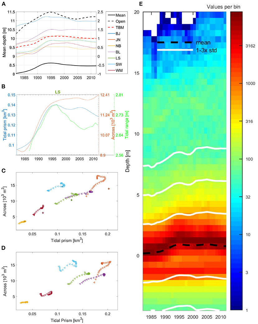
Figure 2. (A) Mean depth (left y-axis) in the area covered by the AufMod data (thick black line) and in the open ocean (thick black dashed line; see Figure 1B for the definition of “open ocean”). The mean depths of individual tidal basins (right y-axis) are shown with colors (see legend and Figure 1B for their definition). The tidal basin mean (TBM) is shown with the thick red dashed line (right y-axis). (B) Tidal prism (blue), cross-sectional area of the Otzumer Balje (red), and tidal range (green; see Figure 1B for the positions of the tidal gauges). The tidal range used to compute the tidal prism is taken as 2.4 m, which is approximately the mean value in front of the NFWS. (C) Scatter plots showing the cross-sectional areas of the individual tidal basins vs. the corresponding tidal prisms. The colors for the individual tidal basins are the same as in (A). Triangular symbols are used for the period 1982–1993. After 1993, circular symbols are used. The + symbols show the changes in 1993 if a uniform deepening of 0.56 m is specified after 1982. (D) Is the same as (C), however the cross-sectional areas and tidal prisms are computed from the numerical model. (E) Shows the vertical distribution of depths (log scale) in the LS area presented as a function of the number of samples per individual depth-time bins. Bins are 0.5 m times 1 year big. The black dashed line shows the mean depth and the white lines show ranges of 1–3 standard deviations. This presentation is stretched in order that the curve of the mean value approximately corresponds to the respective curve of LS area in (A).
The deepening observed north of the barrier islands occurred faster than that in the tidal flats and tidal basins (compare the solid and dashed black lines in Figure 2A). These changes did not occur in phase over different depth ranges or in the individual tidal basins (see the colored lines in Figure 2A). This finding could illustrate (1) a total export of sediment from the region or (2) the redistribution of sediment between the deep and shallow regions and/or between the individual tidal basins. The second phase of the observation period was characterized by sediment accumulation in most of the intertidal basins of the EFWS (see also Benninghoff and Winter, 2019); however, their mean depth did not change much (red dashed curve). Unlike the depth of the shallow area, the open ocean bathymetry deepened after 2005. The bathymetric measurements reveal that the coupled hydrodynamic-morphodynamic system reached an extreme state in 1995, after which the overall trend reversed.
There is a reasonable question of how certain the trends presented in Figure 2A are provided that these data show averages of a very large number of locations. Only for the back barrier basin behind the islands of Langeoog and Spiekeroog do we have 4,500 locations on a map with a resolution of 50 m. To present the morphodynamic changes in a statistically meaningful way, we show in the right-hand-side panel of Figure 2 the number of observations in the LS area in the bin-size grid rather than the individual data. This presentation is a good substitute for presenting individual depths with small dots; in a later presentation, dots would overlap because of the large amount of data. The color bar provides the number of observations in the individual depth-time bins. At each time, the sum of the number of observations over the whole depth range (all bins) equals the total number of observations mapped with a resolution of 50 m. The probability distribution would look the same; however, we prefer to show the number of data points per bin to demonstrate the size of the observations. This presentation is considered a compromise aiming to elucidate the basic characteristics of the depth evolution (dashed line) and the spread of data in the respective ranges of depth. The distribution of the individual observations around the mean is not Gaussian, and the skewness illustrates the fact that areas of relatively larger depths occupy only a very small part of this tidal basin. Notably, the distribution has a diffuse secondary maximum at ~12 m depth. As seen by the comparison of Figure 2A (LS curve) and Figure 2E, the mean curve in Figure 2E is representative of the overall evolution of the LS area. The same conclusions hold for the remaining tidal basins (not shown).
Figure 2B illustrates an example of the bathymetric development in an individual tidal basin (namely, the intertidal basin behind the islands of Langeoog and Spiekeroog), the temporal evolution of the tidal prism (the tidal range was taken as 2.4 m, which is approximately the mean value in front of the NFWS), and the inlet cross-sectional area (orthogonal to the direction of the tidal channel and computed at zero sea level). The relationship between the tidal prism and the inset cross-sectional area is explained by de Swart and Zimmerman (2009). As seen in Figure 2B, there is a clear correlation between these two parameters in the period 1986–1993 (correlation coefficient c = 0.98), after which both of them remained rather constant.
The tidal range could affect the tidal storage (tidal prism) in intertidal basins, and tidal storage can be affected by bathymetric changes. To identify the possible relationships between changes in sea level and bathymetry, we analyzed data from tide gauge stations (see the locations in Figure 1B). The tidal range estimated from these tide gauges in the period 1987–1993 (no data are available before 1987) showed an increase of 4.4–14.6 cm in different intertidal basins. Notably, the results of Wahl et al. (2013) showed an overall positive trend in the mean sea level of the North Sea, which can be indirectly linked to the trend in the tidal range observed in the early 1990s.
The evolution of tidal flats is coupled with the evolution of tidal channels. An increase in the tidal prism would increase the amount of water transported within the inlet. This would tend to increase the speed of currents and promote stronger erosion of the bed, which would increase the cross-sectional area of the inlet. To confirm whether this is the case in our study area, we computed the correlation between the tidal prisms of the individual areas of the tidal basins (Figure 1B) and the corresponding cross-sectional inlet areas (Table 1). The correlation is always higher than 0.7 (minimum of 0.73 for the inlet between Juist and Norderney and maximum of 0.96 for the inlet between the islands of Langeoog and Spiekeroog).
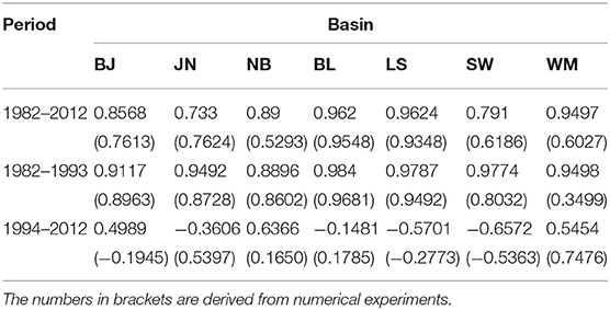
Table 1. Correlation between tidal prism and cross sectional area in individual basins.
The positive correlation between the cross-sectional inlet area and tidal prism for all the intertidal basins of the EFWS (Figure 2C) demonstrates similar morphodynamic responses among all the basins. The different ranges are explained by the different sizes of the individual tidal basins. The increasing trend during 1986–1993 (triangular symbols are used for the years before 1994) is consistent with the parallel evolution of the deep and shallow areas shown in Figure 2A. After 1995 (circular symbols), the changes in the areas of the tidal basins and their corresponding cross-sectional areas remained relatively small. The results in Figure 2C were computed by imposing a uniform tidal range of 2.4 m for all tidal basins. Practically, this figure presents tidal prisms and cross-sections in the inlets as computed from bathymetric data. One can ask whether using a uniform tidal range for all tidal basins is a reasonable assumption. An alternative analysis is presented in Figure 2D, in which sea level is taken from the model as a function of time and space. Obviously, Figures 2C,D are not identical; however, the overall analysis based on the simplified approach used to plot Figure 2C holds. Finally, to estimate possible errors when presenting the results in Figures 2C,D, we compared the transport in the inlets against the time rate of change of the volume of water in the tidal basins, both estimated from the model. The differences between the respective transports are small compared to the magnitudes of their temporal changes.
The slopes of the correlation curves in Figures 2C,D are different in individual tidal basins. Furthermore, the nearly linear correlation during the period 1982–1993 subsequently transforms into a complex relationship between the two characteristics. The first result demonstrates that the cross-sectional area between the islands is most sensitive to the change in the tidal prism of the respective tidal basin. The largest slopes in Figures 2C,D occur in the Juist Norderney (orange) and Wangerooge Minsener Oog (red) areas. In contrast, the inlet between Baltrum and Langeoog (the most horizontal curve, plotted in purple) is less sensitive to the change in the tidal prism. In addition, the change in the type of correlation after 1993 could indicate a rapid transition of the morphodynamic state during the first period (akin to an adjustment to a new state), followed by natural evolution during the second phase, during which the migration of channels was more pronounced than the overall deepening (see Table 1). The individual estimates of the linear relationship between the tidal prism and the cross-sectional area in the cases shown in Figures 2C,D are summarized in Table 1, where the numbers in brackets show the results in the case when the minimum and maximum volumes of intertidal basins and the respective cross-sections are computed from the model.
The above estimates could be affected by observation errors. To (at least partially) exclude this possibility, we estimated the hypsometric relationships corresponding to a uniform deepening of 0.56 m in the bathymetry of the entire area; that is, we prescribed a mean deepening of 0.56 m for the entire area during the period 1981–1993. The depth of the hypothetical 1993 state is shown by the “+” symbols on the phase diagram. Obviously, a uniform change in bathymetry is in most cases far from the observed change. Only for the intertidal basins of Norderney Baltrum and Baltrum Langeoog do the “+” symbols overlap the main observed trend. This result can serve as partial proof that a constant error in bathymetric data cannot explain the results discussed above. It is more plausible that the data describe real (consistent) morphodynamic changes.
Another source of errors could originate from the sampling strategy. Notably, measurements were not carried out every year over the entire area bordered by the red line in Figure 1A. The area between the red dashed and red full lines in this figure is where the time interval between individual observations is longer than 2 years on average. These are mostly the areas in front of the eastern coast, which are close to the open ocean. In most of the Wadden Sea, measurements are carried out every year. With respect to possible deficiencies in the interpretation of the modeling results, we want to point out that for the times when data were not available from observations, the DEM was interpolated. To illustrate the high quality of the data, we show in Figure 3 a zoomed bathymetry in the area of the mouth of the Elbe Estuary. Obviously, the major bathymetric changes there are associated with the migration of small tidal channels, as well as with their branching or disappearance and formation of new channels (Figure 4).
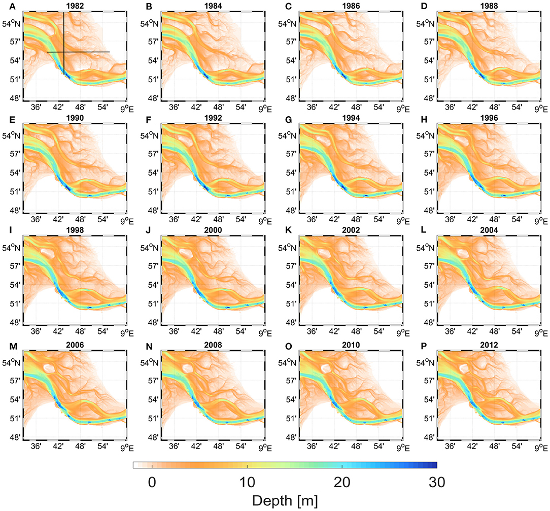
Figure 3. Temporal-spatial evolution of the bathymetry west of the Elbe Estuary illustrated as consequent bathymetric maps plotted for every second year (A–P). Black lines in (A) show locations of meridional and zonal transects, for which the bathymetric development is shows as time vs. distance diagrams in Figure 4.
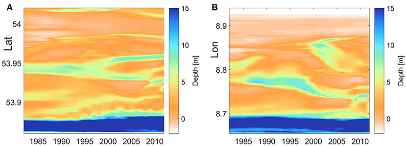
Figure 4. Time vs. distance diagrams of bathymetry west of the Elbe Estuary along meridional (A) and zonal (B) sections shown in Figure 3A.
3.2. Hydrodynamic Responses
3.2.1. Sea Level Rise Experiments
As shown by previous numerical experiments (for references, see Schindelegger et al., 2018), the regional responses to SLR vary considerably among different areas of the global ocean. This is explained by the fact that a reduction in frictional damping at higher water levels (deeper bathymetry) would signify weaker currents and reduced bed shear stresses, thereby explaining the M2 increases in the Irish and Celtic Seas, as well as in the German Bight. As shown by Pickering et al. (2012), in the southeastern German Bight and Dutch Wadden Sea, the amplitude of the M2 constituent increases with SLR.
To evaluate the plausibility of our simulations and their agreement with similar previous simulations addressing the changes due to SLR of 2 m, we first used the model presented by Jacob et al. (2016) and performed two runs. The first run is called NS-1982 (NS-1982 denotes North Sea, 1982 bathymetry); the second run is called NS-SLR-2 (NS-SLR-2 denotes North Sea, sea level rise of two meters). For the nomenclature of experiments (see Table 2). These two experiments were carried out as barotropic experiments (temperature and salinity were kept at constant values of 4 degrees Celsius and 0 psu, respectively). The bottom topography in NS-SLR-2 was deepened by 2 m compared to the bathymetry of NS-1982; this deepening can be considered the equivalent of an SLR of 2 m. The difference between the sea level amplitudes in the two experiments (Figure 5A) agrees with the results presented by Pickering et al. (2012). The coastal zone of the German Bight is among the areas where the response of the sea surface height (SSH) to SLR is strongest.
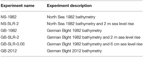
Table 2. Nomenclature of barotropic experiments analyzing the effects of SLR.
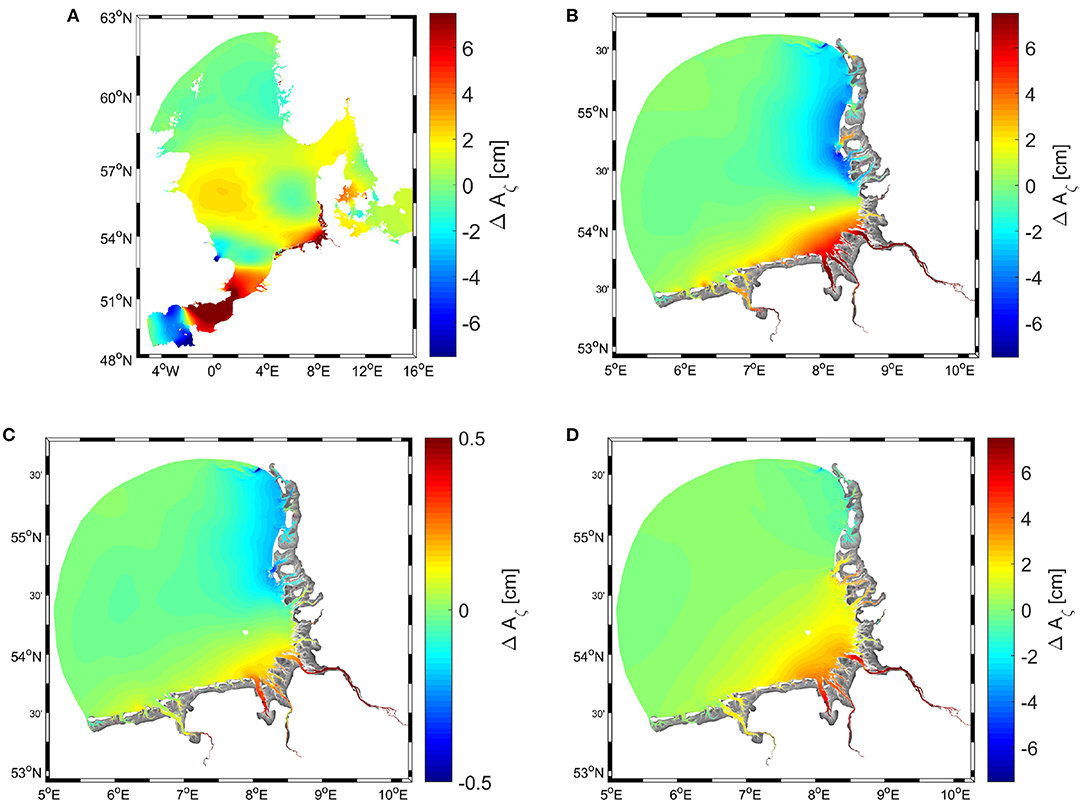
Figure 5. Differences in SSH between the NS-SLR-2 and NS-1982 experiments. Amplitudes are measured as the standard deviation of SSH in the individual experiments during two neap/spring tidal cycles. (B) Is the same as (A) but for the German Bight; here, the comparison is between experiments GB-SLR-2 and GB-1982. (C) Comparison of the amplitudes in GB-SLR-006 and GB-1982. (D) Difference between the amplitudes in GB-2012 and GB-1982.
Figure 5B is the same as Figure 5A but presents the difference between the SSH for experiments GB-SLR-2 and GB-1982, which are the same experiments as NS-SLR-2 and NS-1982 but with “NS” replaced by “GB” (representing the German Bight). These GB experiments were performed to study the response of the SSH in the German Bight to an SLR of 2 m and to compare the results with the NS experiments to ensure that the open boundary condition does not excessively affect the results. A comparison between Figures 5A,B shows that this is approximately the case.
As stated above, the SLR within the studied period of 31 years reached only ~6 cm. Therefore, we repeated GB-SLR-2 as GB-SLR-0.06; that is, we deepened the topography in the entire basin by only 6 cm. The difference pattern is almost the same as in Figure 5B, but the amplitudes in Figure 5C are much lower (note the different contour intervals in Figure 5C). This finding agrees with the earlier conclusions of Pickering et al. (2012) and Idier et al. (2017), who reported that the increases in the high tide levels on the European Shelf are generally proportional to the magnitude of SLR (as long as the SLR is below 2 m).
Finally, we performed an additional barotropic experiment (GB-2012) with the topography taken from the AufMod observations in 2012. One important conclusion is that the bathymetric changes in a relatively small part of the model area (see Figure 1) resulted in a response comparable to that caused by SLR of 2 m (compare Figures 5B,D). However, the bathymetric changes happened at a rate of 44.8 mm/yr, which is ~20 times larger than SLR of the World Ocean (2 mm/yr). This finding provides important justification to more thoroughly analyze the response of the model to time-referenced bathymetry.
3.2.2. Dynamic Responses to Bathymetric Changes
3.2.2.1. Open Ocean
The patterns of the M2 and M4 tidal constituents computed from the tidal analysis of SSH in all simulations with time-referenced bathymetry are qualitatively similar and follow the patterns presented by Stanev et al. (2014) (shown in their Figures 4A,B and therefore not reproduced here). The differences between the individual simulations identify the responses of tides to bathymetric changes in the AufMod area. These differences are presented in Figures 6A,B by the standard deviations of the M2 (a) and M4 (b) tidal amplitudes in the individual experiments. The largest tidal response to the varied bathymetry occurs along the eastern boundary, which is the region of tidal reflection and refraction (Stanev et al., 2014). The magnitudes of these responses largely exceed the magnitudes of responses to SLR (compare to Figure 5). Secondary response maxima appear in the area between the Weser and Elbe Estuaries (for the M2 tide) and north of the Ems Estuary for the M4 tide. The ratio between the amplitudes of the M4 and M2 tides is known to reveal tidal asymmetry. In our 31 response experiments, the ratios between the patterns in Figures 6A,B, which are shown in Figure 6C, identify the areas where tidal asymmetry is most sensitive to bathymetric changes, namely, between the southern tip of the island of Sylt and the Eider Estuary, along the eastern coast, and north of the Ems Estuary in the EFWS.
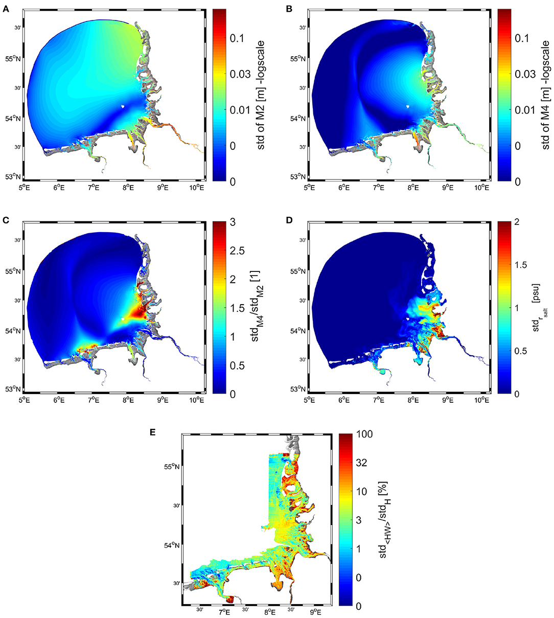
Figure 6. Standard deviations of the amplitudes of the M2 (A) and M4 (B) tides in the experiments with time-referenced bathymetry. (C) Shows the ratio between (B) and (A). The average bathymetry in an area that fell dry in any of the simulations is shown in grayscale. (D) Standard deviation of the surface salinity range. The range (rsalt) is defined as the difference between the absolute minima and maxima of the surface salinity in an individual run. (E) Standard deviation of mean high water normalized by the standard deviation of depth.
A principal difference is observed between the responses of salinity to the bathymetric changes within the EFWS and NFWS (Figure 6D). This can be explained by the fact that most fresh water enters the German Bight from the Weser and Elbe Rivers and propagates northward along the eastern coast. Therefore, the largest anomalies between the individual experiments appear approximately in the same areas where the maximum variations in the ratio between the M4 and M2 tidal amplitudes are observed.
Here, a fundamental question arises as to whether the individual responses described above are local or extend over larger areas. To answer this question, we show in Figure 6E the ratio between the standard deviation of the high water level and the standard deviation of the bathymetry. This ratio can be understood as a measure of the response signal (high water) against the input signal (bathymetry). Obviously, the patterns in Figure 6E differ considerably from the smooth patterns shown in Figures 6A,B. These normalized response patterns show minima in the tidal channels, which is explained by their migration (large bathymetric variability). In contrast, the maxima of the relative (normalized) variability occur in tidal basins and tidal flats surrounding the channels of the NFWS. Particularly strong are the local responses in the Jade-Weser region and in Ems-Dollart Bay.
3.2.2.2. Wadden Sea
The EFWS is known as a representative system comprising multiple tidal basins with similar hypsometric features. The transport properties in the inlets connecting the intertidal basins and open ocean reflect the volumetric characteristics of basins and the cross-sectional areas of the inlets. These transport conditions were analyzed by Stanev et al. (2003, see their Figure 7) and are reproduced in Figure 7A for 1982. The good qualitative agreement between the previous and present simulations is explained by the similar bathymetry used in both studies. Although the magnitudes of transport vary largely from inlet to inlet, once normalized by the corresponding maximal transport curves, the magnitudes converge (Figure 7B). The inflection point (marked by the arrow), which occurs at a low water level, reflects the nonlinear behavior of the Helmholtz oscillator (for more details, see Stanev et al., 2003). This is explained by the change in the area of intertidal basins as a function of SSH, which generates harmonics in the transport with twice the M2 frequency. The asymmetry of the transport curves (the sum of M2 tides and overtides) in the tidal basins of the EFWS (Stanev et al., 2003) is such that the time of transition from peak flood to peak ebb is shorter than the time it takes for the currents to change from peak ebb to peak flood (Figure 7C).
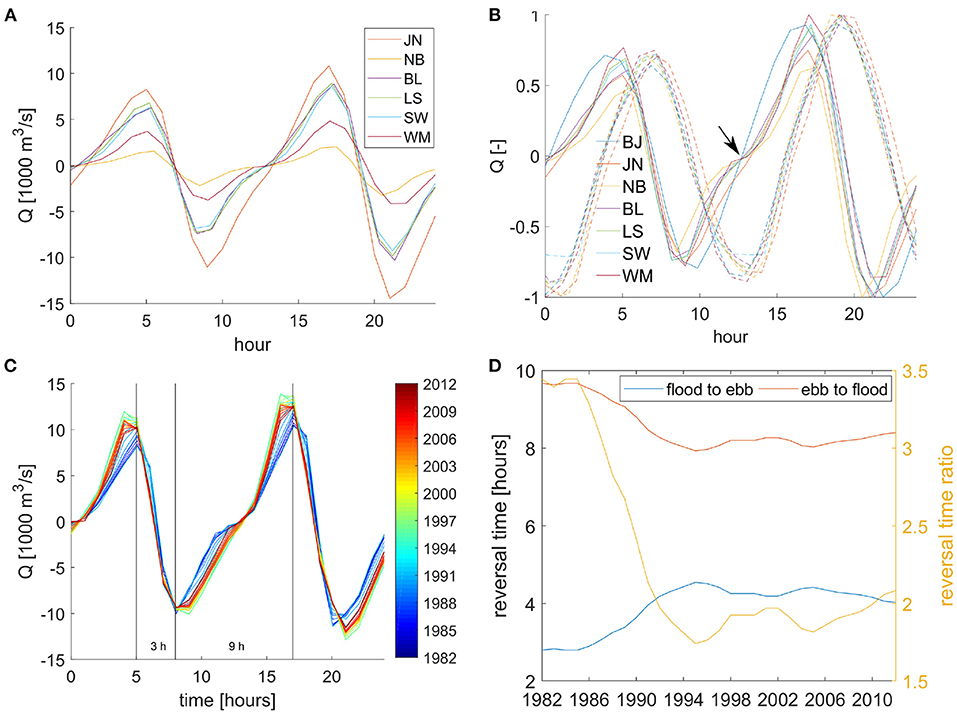
Figure 7. Transport (positive is flood-directed) through the inlets of the EFWS (A) and their corresponding normalized curves (B) for two M2 tidal cycles in 1982. The dashed lines in (B) shows the normalized sea level curves. The arrow marks the inflection point during transition from peak ebb to peak flood velocity. (C) Transport in the inlet between the islands of Langeoog and Spiekeroog for the different years (colors). (D) Estimates of the durations of peak flood to peak ebb vs. peak ebb to peak flood asymmetry. The curve for the intertidal basin behind the islands of Borkum and Juist is not shown in (A) because of the much larger amplitude. To better compare the individual curves in (A,B), the phases have been shifted.
Only the curve characterizing the transport between the islands of Borkum and Juist diverges from the other curves, suggesting that the nonlinear response is not dominant there. This could be due to the different size of this basin and the large exchange with the intertidal basin west of Borkum and Juist; alternatively, this may be due to the rather arbitrary specification of the basin shape or (most likely) to the double inlet system.
What has not been studied previously is the temporal evolution of water transport in the inlets caused by bathymetric changes. Figure 7C shows that the transport in the inlet between the islands of Langeoog and Spiekeroog in individual years deviates from year to year. The asymmetry (shorter peak flood to peak ebb period) was more pronounced in the 1980s, and the inflection point was clearer. This demonstrates that, at these times, the nonlinear tidal response associated with flooding and drying was more pronounced.
Transport asymmetry is known to affect sediment dynamics; therefore, the role of this characteristic in morphodynamic change is of utmost importance. A shorter peak flood to peak ebb period promotes ebb dominance, which causes seaward sediment flushing and sediment export from intertidal basins. Figure 7D illustrates how much the shorter flood to ebb and longer ebb to flood periods have changed. Their ratio halved during the times considered in the present study, particularly before 1995, after which the ratio varied between 1.5 and 2.
Tidal asymmetry can also be measured by the ratio of maximum flood to maximum ebb velocities, called the peak current asymmetry. The temporal evolution of the peak current asymmetry in all inlets in the EFWS (Figure 8) presents the temporal development of the maximum flood and ebb velocities, as well as their ratio. At the beginning of the studied period, the maximum ebb velocities exceeded the maximum flood velocities for all inlets; that is, all intertidal basins were ebb-dominant. With the exception of the Borkum and Juist areas, the ebb-dominated asymmetry weakened until 1995. In some of the tidal basins (Baltrum Langeoog, Langeoog Spiekeroog, and Spiekeroog Wangerooge), the tidal asymmetry changed to flood dominant. These changes illustrate the response of individual basins to bathymetric changes (Figure 2A) and suggest that the flushing trend noted in the 1980s was either reduced or inverted in the second half of the period of bathymetric observations.
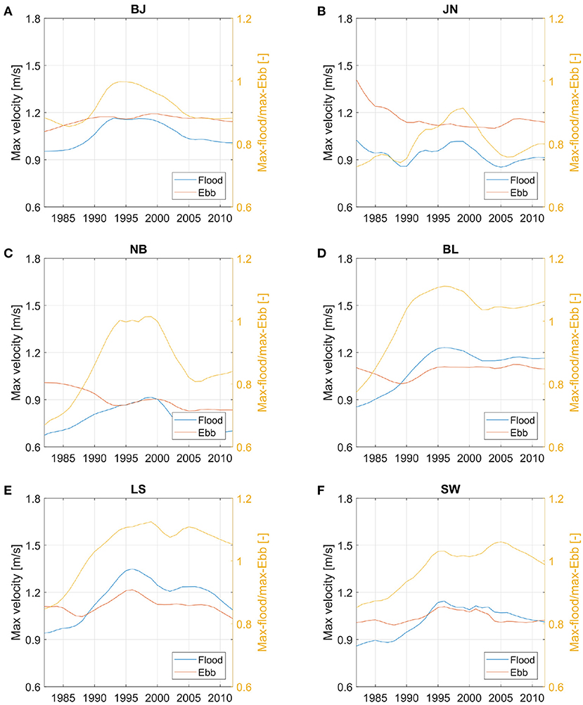
Figure 8. Maximum flood and ebb velocities in the tidal basins of the EFWS: (A) Borkum Juist (BJ), (B) Juist Norderney (JN), (C) Norderney Baltrum (NB), (D) Baltrum Langeoog (BL), (E) Langeoog Spiekeroog (LS), and (F) Spiekeroog Wangerooge (SW).
The peak current asymmetry shows pronounced spatial differences (Figure 9A). The area of flood-dominated asymmetry in the outer part of the model area is bisected by a zone of ebb-dominated asymmetry starting from the Elbe Estuary and approximately following the submerged Elbe Valley. The differences between the spatial patterns in 1982 and 2012 are not well pronounced in the large-scale map; therefore, magnified views of the NFWS and EFWS are provided in Figures 9B,C, respectively. A trend of the decreasing strength of ebb dominance is well-pronounced in the EFWS and is very strong in the Baltrum Langeoog zone, where the currents in the entire intertidal basin became flood-dominated, implying that these changing dynamics contributed to refilling this basin. The patterns in the intertidal basins are patchy overall, demonstrating mixed asymmetry on the tidal flats with a tendency toward flood dominance on the shallows and ebb dominance approaching the main channels. In conjunction with the reduction in ebb asymmetry in the channels from 1982 to 2012, the flood dominance on the flats was also weakened.
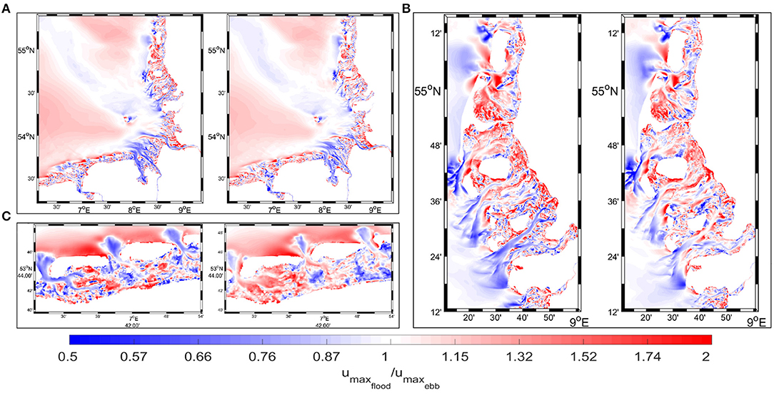
Figure 9. Ratio between the maximum flood and ebb velocities in the German Bight (A) and magnified views of the NFWS (B) and EFWS (C). The 1982 situation is shown on the left; the 2012 situation is shown on the right.
The relative change of the peak current asymmetry expressed as the ratio between the peak current asymmetry during spring tide and the peak current asymmetry during neap tide for 1982 and 2012 (see Supplementary Figure 3) demonstrates a tendency of an increased ebb dominance (respectively reduced flood dominance) in the order of ~10–20% for most of the EFWS. However, at the seaward ends of the estuarine channels, and over the watersheds of the tidal basins, the flood asymmetry is enhanced. The observed reduction of the ebb asymmetry within the two southern most tidal channels of the NFWS is opposite to what is observed in the inlets of the EFWS. This finding illustrates that the spring-neap variations of the peak current asymmetries are regionally rather complex.
One very clear difference in the peak current asymmetry between the EFWS and NFWS is the simpler oceanward structure of the barrier islands. In the EFWS, the flood asymmetry increases toward the islands; the individual zones are separated by zones of ebb-dominant asymmetry coinciding with the tidal channels. East of the NFWS, the tidal asymmetry is predominantly ebb-dominated, which reduces slightly with increasing distance from the coast. This can partially be explained by the different morphologies. Notably, east of the island of Sylt, which can be considered an analog to the barrier islands in the EFWS, the asymmetry is ebb-dominant. Toward the coast and around the individual islands, patches of flood or ebb asymmetry are mixed, reflecting the complex patterns of bathymetry and tidal flats. The NFWS region follows the overall trend of asymmetry of either direction decreasing in strength from 1982 to 2012; only for the Eider Estuary is the ebb asymmetry partially enhanced. Ending this analysis, we remind the reader that tidal current asymmetry only serves as a proxy for trends in morphodynamic evolution. It can also have different meanings for sediment dynamics depending on depth (whether currents are meaningful for bed mobility) or proximity to an area of resuspension.
3.2.2.3. Estuaries
Changes in tidal characteristics within the German Bight have been recognized for many years (Jensen and Mudersbach, 2007). The reasons for these changes, however, are less well-understood, particularly regarding natural changes. We have already shown that the changes in the German Bight and Wadden Sea are associated with bathymetric variations. Here, we more closely investigate the situation in estuaries to diagnose the responses to bathymetric changes in the Ems, Weser, and Elbe Estuaries resulting from changes in bathymetry (Figures 10A,D,G). Because the AufMod dataset does not extend far up rivers, the deepening of estuaries as a result of human interventions in these areas is not (fully) accounted for.
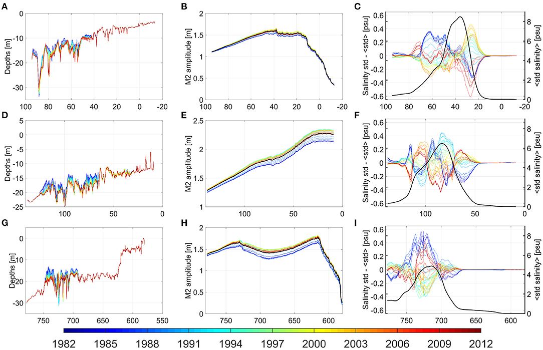
Figure 10. Bathymetric changes in the Ems (A), Weser (D), and Elbe (G) Estuaries. The corresponding amplitudes of the M2 tide are shown in the middle (B,E,H), and the variability of the sea surface salinity is shown on the right. The individual colors represent individual years. Wherever, the bathymetry in the AufMod data does not cover some areas, the color is red. The black lines in the figures in the middle and on the right show the mean of the standard deviations (M2 amplitudes in the middle panels) for all experiments with time-referenced bathymetry. The colored lines in (C,F,I) depict the difference between the standard deviation in the individual experiment and the mean standard deviation.
The changes in the M2 tide in the Ems Estuary (Figure 10B) are relatively small. This contradicts the fact that in recent decades, the tides in this estuary have changed considerably, even changing the sediment dynamics and creating conditions to form a persistent fluid mud layer. The absence of such responses from our simulations implies that the observed changes are due to modification of the riverbed upstream. In contrast, bathymetric changes in the area of the river mouth (the area of available time-referenced bathymetric data) have relatively small impacts on the tides in the Ems Estuary.
Changes in the M2 tide in the Weser and Elbe Estuaries caused by bathymetric changes reach up to ~20 cm, occurring mostly in the period 1982–1995, after which the tidal amplitudes changed only slightly. Notably, these changes propagate far beyond the area where bathymetric changes are prescribed; that is, the effects are not just local. These effects include not only the variation in the M2 amplitude along the thalweg, which is quite different among the three estuaries (Figures 10B,E,H) but also the position of the maximum sensitivity to the bathymetric changes. These changes are small in the Ems Estuary; in contrast, the differences between the tidal ranges continuously increase with increasing distance from the ocean in the Weser Estuary, and the maxima are approximately in the middle of the Elbe Estuary.
The variability in sea surface salinity (black curves in the panels on the right in Figure 10) illustrates the position of the salinity front. The amplitudes reach 8 psu in the Ems Estuary and ~5 psu in the Elbe Estuary. As known from the simulations with the same model as that of Stanev et al. (2019), the estuarine turbidity maximum is observed in this area. The present numerical simulations reveal that the difference in the salinity variability between the individual years reaches ~10–20% of the mean. We conclude that the sharpness of the salinity front changes, which can strongly affect the sediment dynamics in estuaries. Moreover, because the sediment dynamics in natural systems are coupled with morphodynamic changes, numerous feedback mechanisms could occur. Our diagnosis only quantifies the possible ranges of changes in tides and salinity, which would affect the morphodynamics in the study area.
Experiments with the same model but coupled with sediment (Stanev et al., 2019) demonstrated that density effects on stratification caused by high sediment concentrations resulted in a suppression of turbulence and a further increase in the concentration of suspended matter at the bottom. In this way, the sediment concentration at the bottom can reach values typical of hyperturbid environments. This is the case of the Ems Estuary. In the remaining part of the model area, sediment concentration does not greatly affect density; therefore, one could conclude that the above analyses of hydrodynamic responses to bathymetric change hold.
4. Discussion
One fundamental question we must ask concerns the realism of the morphological development observed in the AufMod data and the corresponding numerical simulations. Errors in the mapped data cannot be excluded due to either the quality of observations or the area coverage. Fortunately, the analysis of the observational data and numerical simulations helped to avoid misinterpretation. This is particularly important for the initial period of observations when the data coverage and quality was not as good as in the 1990s and 2000s. During this period, the bathymetric depth in the entire area covered by the AufMod data increased rapidly, which brings the realism of these data into question. However, in this period, the morphological evolution exhibited some regularities (Figure 2), such as the good correlation between the tidal prisms and the cross-sectional areas of the inlets (Figures 2C,D and Table 1). Furthermore, the temporal evolution of each individual basin followed a very regular pattern, and the scatter of this relationship (Figure 2C) was small. The experiment involving a constant increase in the depth over the whole area with respect to the depth in 1982 demonstrated that such a “manipulation” of the bathymetry is dynamically far from the natural evolution described by the observational data.
Another test of the data consistency was provided by the numerical simulations. It is well-known that changes in the flood and ebb currents in the tidal inlets of the EFWS are controlled by the tidal prisms and cross-sectional areas of the tidal basins and inlets. The simulations demonstrated that the type of tidal asymmetry changed rapidly (or even reversed) in the 1990s. As the combination of deep tidal channels and shallow flats favors the development of ebb/flood asymmetry on channels/shoals, this deepening trend triggered a reduction in the peak current asymmetry, presenting a change in the morphological driver. In a model accounting for morphodynamics, this would lead to refilling of the intertidal basins with sediment, which can be considered a natural reaction to rapid deepening.
Bathymetric evolution is a very complex issue. To tackle this issue, one needs to bring together hydrodynamics, sediment dynamics and morphodnamics, along with appropriate information about the forcing conditions. Although in the present study we focused only on the hydrodynamics under specified bathymetric conditions, the multiple aspects of the problems were a real challenge. The compromise to focus on hydrodynamic responses only resulted in some constraints on the analysis and study findings. Nevertheless, the number of interpretations consistent with the physical oceanography of coastal oceans demonstrated that the numerical model used herein can be considered a good tool to be coupled with a morphodynamic module. The coupling of this model with a sediment module was already presented by Stanev et al. (2019). One technical problem is that the present model is rather large, containing 475 k nodes and 940 k triangles; in addition, integration over periods spanning a decade or more is computationally challenging. The greater challenge, however, is to use a credible morphodynamic model that adequately replicates the evolution (over all time scales) of the morphological state in the German Bight. Because such a model is still not available, we carried out our diagnostic study as a first step in this direction. The results presented herein justify this approach. Our findings provide clear indications that one precondition for adequate numerical simulations in the coastal ocean is the use of adequate (time-referenced) bathymetry. This would require present-day bathymetries and the data used to compute them to be reconsidered and, wherever possible, time-referenced DEMs to be prepared. More importantly, campaigns should be organized to regularly observe future changes in coastal bathymetry and establish datasets for individual years. This is very important for future morphodynamic modeling, where appropriate data are needed for both model initialization and model validation. The absence of such data remains an obstacle to developing morphodynamic models for coastal zones.
The final point to address here concerns scenario studies, which are of great theoretical and practical interest. When applied to the coastal ocean, scenario studies usually specify a certain SLR (natural change) or deepening of tidal rivers (man-induced changes). As we demonstrated, the effects of natural bathymetric changes can far exceed those of SLR. Only the deepening of tidal rivers without accounting for natural bathymetric changes can reduce the credibility of such scenario studies.
5. Conclusion
The large-scale bathymetric changes in the coastal areas of the German Bight showed a deepening trend in the 1980s and in the early 1990s; in contrast, in the late 1990 and 2000s, most bathymetric changes were characterized by rather small spatial scales and were associated mostly with the eastward migration of tidal channels. High correlations were found between the tidal prisms in the individual tidal basins of the EFWS and the cross-sectional areas of their inlets. However, the corresponding relationships appeared very different among the individual basins. Time slice experiments with the time-referenced bathymetry of the German Bight over three decades using an unstructured grid model demonstrated the following. (1) The responses to bathymetric changes far exceeded the response to SLR. (2) The overall dynamic response to bathymetric changes was, to a large degree, local. However, the eastern (reflective) coast appeared to be more sensitive. In part because of the specific distribution of freshwater sources, the sea surface salinity along the eastern coast also underwent substantial changes due to changes in bathymetry. These were some of the basic diagnostics of the historic development of hydrodynamics in the Waden Sea.
The nonlinearity of the tidal dynamics in the intertidal basins due to hypsometry was strongest in the 1980s and constantly decreased in the late 1990s and 2000. This was followed by a substantial change (even a reversal in some inlets) in tidal asymmetry, which exhibited very complex behavior in the shallow ocean, reflecting the complex changes in forces that drive morphodynamics. It was demonstrated that not only the barotropic dynamics in estuaries were affected by bathymetric changes but also the dynamics of the salinity front. The latter is of crucial importance for the dynamics of estuarine turbidity maxima.
We hope that the present study made one first (diagnostic) step toward numerically simulating and understanding the morphodynamics in coastal zones. The practical message is that wherever possible, numerical modeling of the near-coastal zone must employ time-referenced bathymetry. More importantly, the progress of morphodynamic modeling in realistic ocean settings with large scales and varying bottom forms is strongly dependent on the availability of bathymetric data with appropriate temporal and spatial resolution. In other words, modeling exercises without having good data will have limited success. Therefore, advancing bathymetric data collection is an important prerequisite for the transition from process-oriented modeling to more operationally and practically oriented studies. As shown in other fields of oceanography, having adequate modeling and observations at the same time could work synergistically.
Data Availability Statement
The AufMod bathymetry data used to create the bathymetry time slices can be accessed via the Bundesamt für Seeschifffahrt und Hydrography (ftp://ftp.bsh.de/outgoing/AufMod-Data/CSV_XYZ_files/). The 7 km Atlantic Margin Model data used as boundary forcing was originally obtained via the download servers of the copernicus marine service program (https://marine.copernicus.eu/), but is not available on the platform anymore for the here used 2012 period in full hourly resolution. Copies of these data exist at Helmholz–Zentrum hereon. Atmospheric forcing data is available upon request from the German Weather Service DWD. Tide gauge and river run off data are available partially directly and partially via request from the data servers of the Federal Waterways and Shipping Administration (WSV, https://www.kuestendaten.de/, https://www.pegelonline.wsv.de). The output of the model simulation performed in the context of this study can be made available after request to the corresponding author.
Author Contributions
ES provided the concept of the paper. BJ created the numerical setups and conducted the numerical simulations. BJ and ES analyzed the results and wrote the paper.
Funding
This work has received funding from the European Union's H2020 Programme for Research, Technological Development and Demonstration under Grant Agreement No: H2020-EO-2016-730030-CEASELESS.
Conflict of Interest
The authors declare that the research was conducted in the absence of any commercial or financial relationships that could be construed as a potential conflict of interest.
Acknowledgments
We thank the German Federal Maritime and Hydrographic Agency (BSH), the Federal Waterways Engineering and Research Institute (BAW) and the other AufMod partners for providing the bathymetric data. We thank the Federal Waterways and Shipping Administration (WSV), the German Weather Service (DWD) and the partners of the Copernicus program for providing the atmospheric and hydrographic data used to force our model. We thank Agustin Sanchez-Arcilla and the three reviewers for their comments, which helped to further improve the manuscript.
Supplementary Material
The Supplementary Material for this article can be found online at: https://www.frontiersin.org/articles/10.3389/fmars.2021.640214/full#supplementary-material
References
Benninghoff, M., and Winter, C. (2019). Recent morphologic evolution of the German Wadden Sea. Sci. Rep. 9:9293. doi: 10.1038/s41598-019-45683-1
Dam, G., Wegen, M. v. d., Labeur, R. J., and Roelvink, D. (2016). Modeling centuries of estuarine morphodynamics in the Western Scheldt estuary. Geophys. Res. Lett. 43, 3839–3847. doi: 10.1002/2015GL066725
de Swart, H., and Zimmerman, J. (2009). Morphodynamics of tidal inlet systems. Annu. Rev. Fluid Mech. 41, 203–229. doi: 10.1146/annurev.fluid.010908.165159
Dieckmann, R., Osterthun, M., and Partenscky, H. W. (1987). Influence of water-level elevation and tidal range on the sedimentation in a German tidal flat area. Prog. Oceanogr. 18, 151–166. doi: 10.1016/0079-6611(87)90031-0
Dronkers, J. (1986). Tidal asymmetry and estuarine morphology. Netherl. J. Sea Res. 20, 117–131. doi: 10.1016/0077-7579(86)90036-0
Ferrarin, C., Cucco, A., Umgiesser, G., Bellafiore, D., and Amos, C. L. (2010). Modelling fluxes of water and sediment between venice lagoon and the sea. Contin. Shelf Res. 30, 904–914. doi: 10.1016/j.csr.2009.08.014
Flemming, B. W. (2002). “Effects of climate and human interventions on the evolution of the wadden sea depositional system (southern North Sea),” in Climate Development and History of the North Atlantic Realm, eds G. Wefer, W. H. Berger, K. E. Behre, and E. Jansen (Berlin; Heidelberg: Springer), 399–413. doi: 10.1007/978-3-662-04965-5_26
Friedrichs, C. T. (2011). “3.06 - tidal flat morphodynamics: a synthesis,” in Treatise on Estuarine and Coastal Science, eds E. Wolanski and D. McLusky (Waltham, MA: Academic Press), 137–170. doi: 10.1016/B978-0-12-374711-2.00307-7
Idier, D., Paris, F., Cozannet, G. L., Boulahya, F., and Dumas, F. (2017). Sea-level rise impacts on the tides of the European shelf. Contin. Shelf Res. 137, 56–71. doi: 10.1016/j.csr.2017.01.007
Jacob, B., Stanev, E. V., and Zhang, Y. J. (2016). Local and remote response of the North Sea dynamics to morphodynamic changes in the Wadden Sea. Ocean Dyn. 66, 671–690. doi: 10.1007/s10236-016-0949-8
Janssen, F., Schrum, C., and Backhaus, J. O. (1999). A climatological data set of temperature and salinity for the Baltic sea and the north sea. Deutsche Hydrogr. Zeitsch. 51:5. doi: 10.1007/BF02933676
Jensen, J., and Mudersbach, C. (2007). Zeitliche Änderungen in den wasserstandszeitreihen an den deutschen küsten. Berichte Deutschen Landesk. 81:99.
Lesser, G. R., Roelvink, J. A., van Kester, J. A. T. M., and Stelling, G. S. (2004). Development and validation of a three-dimensional morphological model. Coast. Eng. 51, 883–915. doi: 10.1016/j.coastaleng.2004.07.014
Maas, L. R. M. (1997). On the nonlinear Helmholtz response of almost-enclosed tidal basins with sloping bottoms. J. Fluid Mech. 349, 361–380. doi: 10.1017/S0022112097006824
Milbradt, P., Valerius, J., and Zeiler, M. (2015). Das funktionale bodenmodell: aufbereitung einer konsistenten datenbasis für die morphologie und sedimentologie. Die Küste 83, 19–38.
Müller, M. (2012). The influence of changing stratification conditions on barotropic tidal transport and its implications for seasonal and secular changes of tides. Contin. Shelf Res. 47, 107–118. doi: 10.1016/j.csr.2012.07.003
Müller, M., Arbic, B. K., and Mitrovica, J. X. (2011). Secular trends in ocean tides: observations and model results. J. Geophys. Res. 116, 1–19. doi: 10.1029/2010JC006387
O'Dea, E., Furner, R., Wakelin, S., Siddorn, J., While, J., Sykes, P., et al. (2017). The CO5 configuration of the 7km Atlantic margin model: large scale biases and sensitivity to forcing, physics options and vertical resolution. Geosci. Model Dev. 10, 2947–2969. doi: 10.5194/gmd-10-2947-2017
Pickering, M. D., Wells, N. C., Horsburgh, K. J., and Green, J. A. M. (2012). The impact of future sea-level rise on the European shelf tides. Contin. Shelf Res. 35, 1–15. doi: 10.1016/j.csr.2011.11.011
Pinto, L., Fortunato, A., Zhang, Y., Oliveira, A., and Sancho, F. (2012). Development and validation of a three-dimensional morphodynamic modelling system for non-cohesive sediments. Ocean Model. 57–58, 1–14. doi: 10.1016/j.ocemod.2012.08.005
Ridderinkhof, W., Hoekstra, P., Van der Vegt, M., and De Swart, H. (2016). Cyclic behavior of sandy shoals on the ebb-tidal deltas of the Wadden Sea. Contin. Shelf Res. 115, 14–26. doi: 10.1016/j.csr.2015.12.014
Robins, P. E., and Davies, A. G. (2010). Morphological controls in sandy estuaries: the influence of tidal flats and bathymetry on sediment transport. Ocean Dyn. 60, 503–517. doi: 10.1007/s10236-010-0268-4
Roelvink, D., and Reniers, A. J. H. M. (2011). A Guide to Modeling Coastal Morphology. Singapore; London: World Scientific. doi: 10.1142/7712
Sarkisyan, A. S. (1977). The diagnostic calculations of a large-scale oceanic circulation. Sea 6, 363–458.
Schindelegger, M., Green, J. a. M., Wilmes, S.-B., and Haigh, I. D. (2018). Can we model the effect of observed sea level rise on tides? J. Geophys. Res. 123, 4593–4609. doi: 10.1029/2018JC013959
Schloen, J., Stanev, E. V., and Grashorn, S. (2017). Wave-current interactions in the southern North Sea: the impact on salinity. Ocean Model. 111, 19–37. doi: 10.1016/j.ocemod.2017.01.003
Schrottke, K., and Heyer, H. (2013). Aufbau Von Integrierten Modellsystemen zur Analyse der langfristigen Morphodynamik in der Deutschen Bucht : AufMod; gemeinsamer Abschlussbericht für das Gesamtprojekt mit Beiträgen aus allen 7 Teilprojekten. Technical report, Bundesamt für Seeschifffahrt und Hydrographie (BSH) [u.a.].
Schulz-Stellenfleth, J., and Stanev, E. (2016). Analysis of the upscaling problem-a case study for the barotropic dynamics in the North Sea and the German Bight. Ocean Model. 100, 109–124. doi: 10.1016/j.ocemod.2016.02.002
Stanev, E. V., Al-Nadhairi, R., Staneva, J., Schulz-Stellenfleth, J., and Valle-Levinson, A. (2014). Tidal wave transformations in the German Bight. Ocean Dyn. 64, 951–968. doi: 10.1007/s10236-014-0733-6
Stanev, E. V., Al-Nadhairi, R., and Valle-Levinson, A. (2015). The role of density gradients on tidal asymmetries in the German Bight. Ocean Dyn. 65, 77–92. doi: 10.1007/s10236-014-0784-8
Stanev, E. V., Dobrynin, M., Pleskachevsky, A., Grayek, S., and Günther, H. (2009). Bed shear stress in the southern North Sea as an important driver for suspended sediment dynamics. Ocean Dyn. 59, 183–194. doi: 10.1007/s10236-008-0171-4
Stanev, E. V., Flöser, G., and Wolff, J.-O. (2003). First- and higher-order dynamical controls on water exchanges between tidal basins and the open ocean. A case study for the East Frisian Wadden Sea. Ocean Dyn. 53, 146–165. doi: 10.1007/s10236-003-0029-8
Stanev, E. V., Jacob, B., and Pein, J. (2019). German Bight estuaries: an inter-comparison on the basis of numerical modeling. Contin. Shelf Res. 174, 48–65. doi: 10.1016/j.csr.2019.01.001
Stanev, E. V., Wolff, J.-O., and Brink-Spalink, G. (2006). On the sensitivity of the sedimentary system in the East Frisian Wadden Sea to sea-level rise and wave-induced bed shear stress. Ocean Dyn. 56, 266–283. doi: 10.1007/s10236-006-0061-6
Umlauf, L., and Burchard, H. (2003). A generic length-scale equation for geophysical turbulence models. J. Mar. Res. 61, 235–265. doi: 10.1357/002224003322005087
Wachler, B., Seiffert, R., Rasquin, C., and Kösters, F. (2020). Tidal response to sea level rise and bathymetric changes in the German Wadden Sea. Ocean Dyn. 70, 1033–1052. doi: 10.1007/s10236-020-01383-3
Wahl, T., Haigh, I. D., Woodworth, P. L., Albrecht, F., Dillingh, D., Jensen, J., et al. (2013). Observed mean sea level changes around the North Sea coastline from 1800 to present. Earth-Sci. Rev. 124, 51–67. doi: 10.1016/j.earscirev.2013.05.003
Wang, Z. B., Hoekstra, P., Burchard, H., Ridderinkhof, H., De Swart, H. E., and Stive, M. J. F. (2012). Morphodynamics of the Wadden Sea and its barrier island system. Ocean Coast. Manage. 68, 39–57. doi: 10.1016/j.ocecoaman.2011.12.022
Warner, J. C., Sherwood, C. R., Signell, R. P., Harris, C. K., and Arango, H. G. (2008). Development of a three-dimensional, regional, coupled wave, current, and sediment-transport model. Comput. Geosci. 34, 1284–1306. doi: 10.1016/j.cageo.2008.02.012
Winter, C. (2011). Macro scale morphodynamics of the German North Sea coast. J. Coast. Res. 70, 706–710.
Zhang, Y., and Baptista, A. M. (2008). Selfe: a semi-implicit Eulerian-Lagrangian finite-element model for cross-scale ocean circulation. Ocean Model. 21, 71–96. doi: 10.1016/j.ocemod.2007.11.005
Keywords: German Bight, bathymetry, morphological evolution, tidal asymmetry, sensitivity study, unstructured grid modeling, East Frisian Wadden Sea
Citation: Jacob B and Stanev EV (2021) Understanding the Impact of Bathymetric Changes in the German Bight on Coastal Hydrodynamics: One Step Toward Realistic Morphodynamic Modeling. Front. Mar. Sci. 8:640214. doi: 10.3389/fmars.2021.640214
Received: 10 December 2020; Accepted: 27 April 2021;
Published: 04 June 2021.
Edited by:
Agustin Sanchez-Arcilla, Universitat Politecnica de Catalunya, SpainReviewed by:
Dano Roelvink, IHE Delft Institute for Water Education, NetherlandsMaarten Van Der Vegt, Utrecht University, Netherlands
Copyright © 2021 Jacob and Stanev. This is an open-access article distributed under the terms of the Creative Commons Attribution License (CC BY). The use, distribution or reproduction in other forums is permitted, provided the original author(s) and the copyright owner(s) are credited and that the original publication in this journal is cited, in accordance with accepted academic practice. No use, distribution or reproduction is permitted which does not comply with these terms.
*Correspondence: Benjamin Jacob, benjamin.jacob@hereon.de