Efficacy of Feedforward and LSTM Neural Networks at Predicting and Gap Filling Coastal Ocean Timeseries: Oxygen, Nutrients, and Temperature

Ocean data timeseries are vital for a diverse range of stakeholders (ranging from government, to industry, to academia) to underpin research, support decision making, and identify environmental change. However, continuous monitoring and observation of ocean variables is difficult and expensive. Moreover, since oceans are vast, observations are typically sparse in spatial and temporal resolution. In addition, the hostile ocean environment creates challenges for collecting and maintaining data sets, such as instrument malfunctions and servicing, often resulting in temporal gaps of varying lengths. Neural networks (NN) have proven effective in many diverse big data applications, but few oceanographic applications have been tested using modern frameworks and architectures. Therefore, here we demonstrate a “proof of concept” neural network application using a popular “off-the-shelf” framework called “TensorFlow” to predict subsurface ocean variables including dissolved oxygen and nutrient (nitrate, phosphate, and silicate) concentrations, and temperature timeseries and show how these models can be used successfully for gap filling data products. We achieved a final prediction accuracy of over 96% for oxygen and temperature, and mean squared errors (MSE) of 2.63, 0.0099, and 0.78, for nitrates, phosphates, and silicates, respectively. The temperature gap-filling was done with an innovative contextual Long Short-Term Memory (LSTM) NN that uses data before and after the gap as separate feature variables. We also demonstrate the application of a novel dropout based approach to approximate the Bayesian uncertainty of these temperature predictions. This Bayesian uncertainty is represented in the form of 100 monte carlo dropout estimates of the two longest gaps in the temperature timeseries from a model with 25% dropout in the input and recurrent LSTM connections. Throughout the study, we present the NN training process including the tuning of the large number of NN hyperparameters which could pose as a barrier to uptake among researchers and other oceanographic data users. Our models can be scaled up and applied operationally to provide consistent, gap-free data to all data users, thus encouraging data uptake for data-based decision making.

1. Introduction

Oceans play a pivotal role in the global weather and climate systems and support a multi-billion dollar blue economy, hence continuous monitoring of ocean conditions, in coastal marine areas in particular, is important to a wide range of stakeholders (UNESCO, 2019). Although many different types of observation platforms can measure the same ocean variable (e.g., temperature), there can be fundamental differences between them due to the instrumentation and the spatiotemporal sampling making comparison difficult (Hemming et al., 2020). For example, satellite observations are restricted to the surface and represent area-averages (often over many kilometers) while data from in situ observations represents a point-based observation in space (Lee et al., 2018). Even within the in situ observations, differences exist in terms of the observation depth, spatial coverage and temporal sampling frequency (Bailey et al., 2019). Furthermore, regardless of the type of observation, there are inevitably gaps in ocean timeseries due to various reasons including instrument loss, servicing and repairs, biofouling, deployment schedules, loss of funding etc. (Morello et al., 2014).

These data gaps and inconsistencies make ocean observations inaccessible to non-expert users, and even expert users (e.g., ocean modelers) typically take the path of least resistance when accessing ocean data. It is not a straightforward exercise to compare, for example, recent high frequency (e.g., 5 min) ocean temperature observations from a mooring with sparse (e.g., monthly) bottle data collected in the 1950s (Hemming et al., 2020). Furthermore, timeseries gaps can significantly affect trend analysis (Wynn and Wickwar, 2007).

Savvy data users by comparison, suffer the consequences of non-standardized methods of interpolating these gaps, leading to unaccountable differences in analysis. Furthermore, oceanographers often need gap-free timeseries for a particular analysis, for example, for determining physical mechanisms or teleconnections using empirical orthogonal function (EOF) analysis (e.g., Ashok et al., 2007 or for researching marine heatwaves Schaeffer and Roughan, 2017) since most common heatwave definitions involve comparing temperature anomalies of consecutive days with a climatology constructed from 30 years of daily data (Schlegel et al., 2019). Non-specialists may require gap-free observations concurrent with other timeseries, such as ecological or biological variables (Lee et al., 2019). Finally, measurement of climate impacts (e.g., trends in ocean warming) also necessitates continuous and consistent monitoring of variables over a long period (Malan et al., 2020). However, although ocean observations can date back many decades, there are statistical discontinuities that could be related to changes in ocean observation platforms and practices.

Some ocean observing systems, such as Australia's Integrated Marine Observing System (IMOS, www.imos.org.au) are maturing so as to allow for “learning” of relationships between ocean variables to fill inevitable gaps. Australia has a network of “National Reference Stations” with sampling dating back to the 1940s and 50s (Lynch et al., 2014). Initially sampling was boat based “bottle” sampling, but at the inception of IMOS, this was augmented with moored temperature (electronic sensor) timeseries at 8 m intervals through the water column, since 2008 (Roughan et al., 2010, 2013, 2015), and monthly vertical profiling with an electronic CTD (conductivity temperature and depth meter) sampling every meter. Here we use data from the Port Hacking National Reference Station in 100 m of water off Sydney (34°S) Australia as a case study to demonstrate the use of statistical models for prediction of oxygen and nutrient concentrations and gap filling temperature timeseries data.

Statistical models present an opportunity to fill gaps in observational records using data based approaches that do not involve making assumptions about the underlying physical processes. One such statistical model that has gained popularity in the last decade is the artificial neural network or neural network model (NN) (Emmert-Streib et al., 2020). An NN feeds the input features through numerous neurons arranged in multiple layers to generate an output layer that can be used for solving classification or regression problems (see LeCun et al., 2015 and Emmert-Streib et al., 2020 for more details). Although the first model of a single neuron was proposed in the 1950s (Rosenblatt, 1957), NNs have seen a large resurgence in the last decade partly due to breakthroughs in training efficiency (Hinton et al., 2006). The recent rise in popularity is also due to the development of new models capable of taking advantage of big data to solve real world problems, e.g., involving image recognition (Rawat and Wang, 2017), natural language processing (Young et al., 2018), and timeseries and text analysis (Lipton et al., 2015). See Schmidhuber (2015) and Emmert-Streib et al. (2020) for a detailed account of the historical development of neural networks. These recent breakthroughs in NNs have led to the development of modern open-source programming platforms, such as TensorFlow (developed by Google Brain) (Abadi et al., 2016), PyTorch (developed primarily by Facebook's AI Research Lab), etc. These libraries allow for quick and scalable implementations of state-of-the-art yet “off-the-shelf” NN models.

Due to their success in learning complex relationships, it stands to reason that NNs could be useful for learning the complex spatiotemporal relationships between physical, chemical and biological ocean variables. One of the first applications of NNs in oceanography was by Tangang et al. (1997) to forecast sea surface temperature anomalies of the Niño3.4 climate index. Since then they have been used to assist in forecasting wind generated ocean waves (Makarynskyy, 2005; Tolman et al., 2005), predict sea level fluctuations (Makarynskyy et al., 2004; Han and Shi, 2008), calculate Pacific Ocean heat content (Tang and Hsieh, 2003), statistical downscaling of ocean model output (Bolton and Zanna, 2019), predicting subsurface ocean temperature timeseries (Su et al., 2018; Han et al., 2019; Lu et al., 2019), and ocean eddy detection (Lguensat et al., 2018). Of particular interest to this study is the prediction of water column nutrient concentrations by Sauzède et al. (2017) and Bittig et al. (2018), and creation of virtual marine sensors by Oehmcke et al. (2018). For a comprehensive historical overview of NN applications in oceanography, see Hsieh (2009) and Krasnopolsky (2013).

Despite, their widespread use in Oceanography, examples of NNs that predict nutrients or gap-fill temperatures in the water column (i.e., below the surface) are scarce (exceptions include Sauzède et al., 2017, Bittig et al., 2018, and Fourrier et al., 2020) especially after the breakthroughs in training efficiency in 2006 (Emmert-Streib et al., 2020), and the few studies that do accomplish this do not take advantage of modern frameworks, such as TensorFlow. TensorFlow is an open-end ecosystem/framework for neural network modeling. It contains a suite of tools, libraries/packages, and community resources that are constantly updated with the latest advances in the field of machine learning. It is language agnostic with implementations in Python, R, and Julia, with the Python implementation being the most popular. Furthermore, it allows for the development of models with various levels of abstraction, which means that programmers and researchers new to modeling with NNs can spin up models quickly and easily, and add complexity as they require. Thanks to its large community of machine learning practitioners, researchers in adjacent fields who wish to take advantage of statistical modeling but do not have the knowledge of, or expertise in computer science, can take advantage of latest breakthroughs without worrying about being aware of and downloading latest libraries/packages, and working out compatibility issues. Users must, however, judge the risks of applying such black-box models for themselves and determine the model's suitability to their use case individually. Furthermore, progress has recently been made on the interpretability of neural networks (Lundberg and Lee, 2017; Kwon et al., 2019).

In this study, we demonstrate the efficacy of using “off-the-shelf” NN models built using TensorFlow for modeling dissolved oxygen, nutrient concentrations and temperature throughout the water column at a valuable long-term observational site. We use a simple feedforward neural network to model oxygen and nutrients, however due to the larger amount of data available, we treat temperature modeling as a timeseries prediction problem. For this we use a type of neural network that is adept at modeling timeseries called recurrent neural networks (RNN) (Lipton et al., 2015). RNNs include connections between adjacent timesteps in addition to connections between the input, hidden and output layers. However, typical RNNs struggle to remember long-term dependencies (Graves, 2013) and are also difficult to train (Rosindell and Wong, 2018). Hence we gap-fill temperature using a special type of RNN called a Long Short Term Memory (LSTM) NN (Hochreiter and Schmidhuber, 1997; Adikane et al., 2001) that overcomes both of these shortcomings. As this is a proof of concept study, we outline the NN model design and training in detail. We show the high degree of accuracy that can be obtained when predicting and gap filling using these modern multi-layered NNs. The models developed in this study serve as a proof of concept for applications to other such long term ocean timeseries datasets aiming to create a suite of easy-to-handle, continuous and filled, derived observational products.

This study demonstrates two types of models befitting two datasets with varying characteristics and is hence divided in two parts. First, section 2 describes the two types of datasets, then section 3 details the first model that uses concurrent observations from related oceanic variables to predict dissolved oxygen and nutrient concentrations. The second suite of models detailed in section 4 are used to gap-fill temperature timeseries observations at a single depth over multiple length temporal gaps from days to months using LSTMs.

2. Data

2.1. Prediction Based on Co-variates

Data from discrete depths (“bottle data,” see below) was used for training a simple NN to predict other variables. The “bottle data” consists of measurements of pressure, temperature, salinity, dissolved oxygen and dissolved nutrient concentrations (nitrate, phosphate, and silicate) with timestamps at a long term observation site. The Port Hacking National Reference Station (151.2°E, 34.1°S) is located in 100 m of water, ~8.5 km off the coast of Sydney Australia where tidal influences are weak. See Roughan et al. (2010, 2013, 2015), and Hemming et al. (2020) for more information on the long term sampling at Port Hacking. The water samples are collected in bottles at a range of depths through the water column, nominally, at 10, 20, 30, 40, 50, 75, and 100 m in 100 m of water. The data collection began in 1953 with a frequency of weekly to monthly but due to the nature of manual collection consists of many gaps and irregular sampling intervals. See Hemming et al. (2020) their Figure 3 and Table 1 for a full description of the data collection.

Due to irregularity of the bottle data collection, the prediction problem could not be treated as a timeseries prediction problem but rather as a simple co-variate based prediction problem where time was treated as another co-variate. The timestamps were converted into three co-variates; year, day of the year and hour of the day. This resulted in six predictor variables: pressure, temperature, salinity and the three temporal co-variates. Figures 1, 2 show the relationship between the six co-variates and the Oxygen and Nitrate concentrations, respectively, colored by the pressure at which the measurement was recorded. The Oxygen concentration (Figure 1) is in the range ~160–275 μmol l⁻¹ whereas the nutrients are bounded by 0 μmol l⁻¹ and are heavily skewed to the left. In general, the nutrient concentrations increase with depth and oxygen decreases with depth. A seasonal cycle is evident in the Oxygen concentrations and for the high Nitrogen concentrations. Some inter-annual variability is also visible for both Oxygen and Nitrogen concentrations, albeit the pattern seems less predictable. Since the data were typically collected in the morning Australian Eastern Time (close to midnight UTC time), little useful information is added by the hour-of-the-day co-variate. Models that do not use the hour-of-the-day as an additional co-variate were also tested but the model accuracy remained unchanged. Although most measurements were documented as having been taken at the nominal pressure depths, there are many examples of measurements recorded outside of these nominal depths (Figures 1, 2). As a result, the pressure is treated as a continuous variable.

FIGURE 1

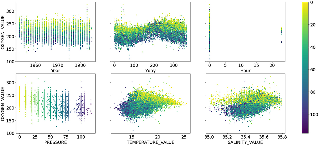
Figure 1. Scatter plots of dissolved oxygen concentration (μmol l⁻¹) (y-axis) against the six co-variates; (from left to right, top to bottom) year, day of the year, hour of the day, pressure (dbar), temperature (°C), and salinity (psu). All points are colored by the pressure value.

FIGURE 2

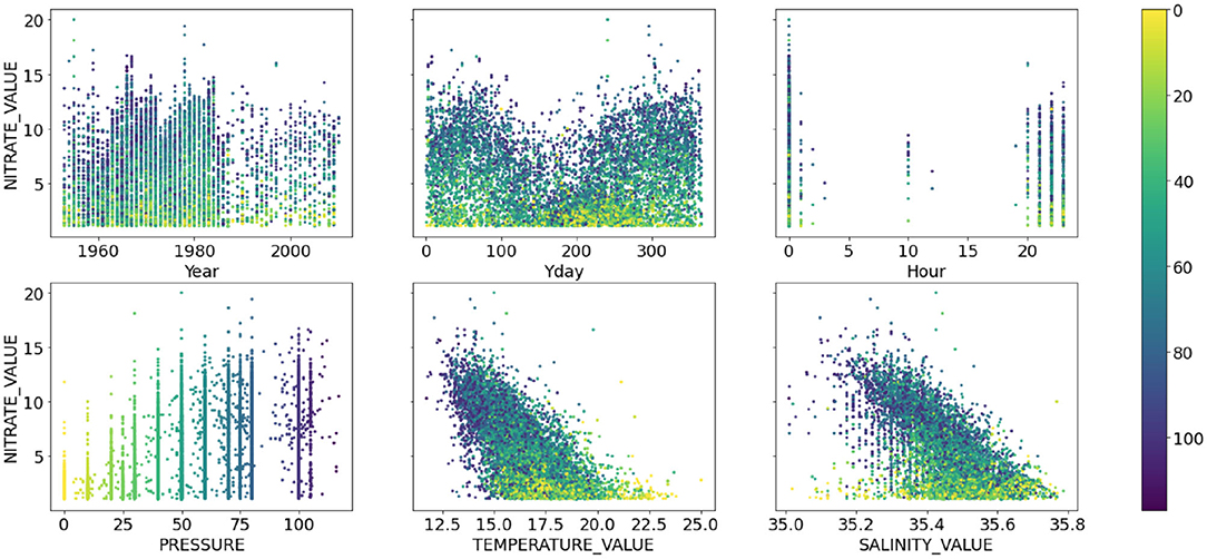
Figure 2. Same as Figure 1 but showing the scatter plots of nitrate concentration (μmol l⁻¹) against the six co-variates.

Data was collected following standard IMOS procedures to ensure data is of high precision and accuracy. IMOS provides guidelines on pre-deployment planning, data collection, post-deployment data processing, and quality control, see Sutherland et al. (2017) for IMOS QA procedures, and Ingleton et al. (2014) and Morello et al. (2014) regarding IMOS quality control (QC). QC includes but is not limited to checking for impossible date, position, depth range (based on global and regional values) correlation with adjacent data (above, below, before, and after). All steps including the use of the IMOS data toolbox for QC are described in Hemming et al. (2020). The data used here were flagged as either “good data” or “probably good data” following UNESCO Intergovernmental Oceanographic Commission (IOC) protocol (flags 1 and 2, respectively) (Lynch et al., 2014; Morello et al., 2014). In addition to the IMOS QA/QC procedures a visual quality control was conducted to remove outliers to aid the model learning process. For example, records corresponding to salinity values below 35 parts per thousand (psu) and above 35.8 psu, pressure above 120 dbar, and nitrate values above 24 μmol l⁻¹ were removed, resulting in 587 records removed for nitrate concentration modeling and 621 records removed for oxygen modeling.

2.2. Gap-Filling Temperature Timeseries

A recurrent neural network model was trained on a “gappy” temperature timeseries obtained from a sensor on a fixed mooring located near the Port Hacking NRS (PH100). The mooring was deployed with AQUATec Aqualogger 520T temperature or 520TP temperature and pressure sensors at 8 m intervals in 2009 to augment the historic bottle data. Temperature data have been acquired using automated electronic senors at 5 min intervals since 2009. Gaps in the temperature data occur through loss of the mooring or sensor failure. The mooring is manually serviced every quarter and has gaps in the timeseries ranging from a few hours, days, to up to 3 months (Table 1). The PH100 mooring was deployed in 2009 and was still operational as of 2020 providing over a decade of temperature observations. Due to the greater number of data samples available, this gap-filling problem was treated as a timeseries prediction problem where the model was trained to predict purely based on the timeseries of the variable of interest, instead of a prediction based on co-variates, as was the case for oxygen and nutrients.

TABLE 1

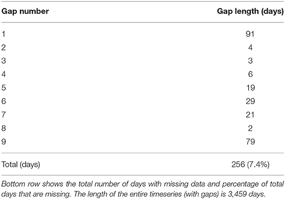
Table 1. Length of gaps in the order they are encountered in the 24.5 m bin temperature timeseries from the Port Hacking 100 mooring.

Since a daily timeseries is adequate for many oceanographic applications, we resample the 5-min observations to a daily frequency using an arithmetic mean. Due to the movement of the sensors, observations are available continuously throughout the water column, with the highest density of measurements available at the optimal depths (the depths at which the temperature sensors are deployed). To find these optimal depths, the daily observations were binned in 1 m intervals and the bins with the highest density of observations were considered as the optimal depths. Since Hemming et al. (2020) showed that the temperature observations at PH100 were highly correlated within 8–9 m, we combined observations from 2 m below and 3 m above the optimal depths and labeled them by the average depth of the resulting range. This results in a regular daily frequency timeseries. For this study, we chose to gap-fill the 24.5 m bin timeseries as a proof-of-concept, which as explained, contains observations between 22 and 27 m. In total, the 24.5 m timeseries contains 3,459 days, with 256 days (7.4% of total timeseries) of missing temperature observations as depicted in Figure 3. These 256 missing days are spread across 9 gaps with the longest gap being 91 days and the shortest being 2 days (Table 1).

FIGURE 3

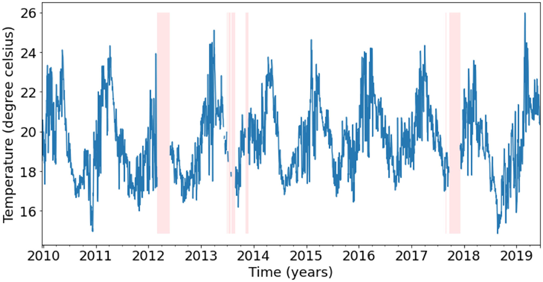
Figure 3. Depiction of the 24.5 m bin temperature timeseries with gaps represented by pink vertical bands. Refer to Table 1 for the lengths of the gaps.

3. Prediction Based on Co-variates

3.1. Model

The simplest, most “vanilla,” neural network known as a feedforward NN consists of many connected nodes or neurons arranged in one or more “hidden” layers (Schmidhuber, 2015). The output of each neuron y consists of a non-linear activation function ϕ applied to a linear function with a weight matrix W and bias vector b.

$\begin{array}{ll}\text{y}=\varphi (W·\text{x}+\text{b})& (1)\end{array}$

Here x is the input vector for the neuron. Training such a NN involves minimizing the loss, which is a function representing how close the NN output is to the true value. Common choices for loss functions include mean squared error (MSE), root mean squared error (RMSE), and mean absolute percentage error (MAPE) for regression problems. There are many optimization algorithms or “optimizers” used to minimize the loss function. One of the most basic but still highly used optimization algorithms is stochastic gradient descent which updates the neuron weights and biases in the direction of the steepest gradient of the loss function during each training step. The size of these parameter updates is determined by a learning rate. All other optimizers are in some sense a variation of stochastic gradient descent. The two most popular variations are RMSprop and Adam which both introduce concepts of adaptive learning rates. See Ruder (2016) and Ketkar (2017) for a complete list of optimizers and their details.

We used a feedforward neural network with four dense, fully connected layers for predicting oxygen, nitrate, phosphate and silicate concentrations, as seen in Table 2. The first three layers contain 64, 64, and 8 nodes, respectively, and the output layer contains one node, which gives the predicted concentration. A Rectified Linear Unit (ReLU) (Nair and Hinton, 2010) activation function was used for the first three layers. The ReLU activation function is a piecewise linear function that returns values equal to its input for positive inputs and zero otherwise. No activation was used for the output layer as no activation is necessary for regression problems. The mean absolute percentage difference (MAPE) between the predicted and the true concentrations was used as the loss function for oxygen prediction and the mean squared error (MSE) was used for nutrient prediction. The Adam optimization algorithm (Kingma and Ba, 2015) was used to minimize this loss function by tuning the node weight parameters. These design choices have been justified further below.

TABLE 2

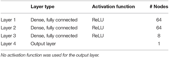
Table 2. Description of the four layer model architecture used to predict dissolved oxygen and nutrient concentrations.

A total of 12,970, 8,633, 12,639, and 6,303 records were used for oxygen, nitrate, phosphate, and silicate concentration modeling, respectively. In all cases 80% of records were chosen at random for the training and validation datasets, and the remaining 20% were used for evaluation of the trained model. The training and validation datasets were also split randomly at an 80–20 ratio.

The model architecture was tested by experimenting with more layers (up to 6) and nodes per layer (up to 1,024), however, more complex models provided little to no improvement to the final model accuracy. Similarly, the hyperparameters were also chosen by experimenting with different values. One of the most important architectural design decisions when tuning an NN is the activation function. As described earlier each node of an NN consists of a linear estimator which is passed through a non-linear activation function to create non-linear estimates (Emmert-Streib et al., 2020). Hence an activation function can influence the decision boundaries and convergence of the NN model. See Table 1 of Emmert-Streib et al. (2020) for a list of the most common activation functions. We tested the ReLU, tanh and sigmoid functions as activations. Although the final validation loss was similar for all three activation choices, ReLU resulted in the smoothest and quickest convergence, with minimal validation dataset loss variability. During training with large datasets, it is often more efficient to take many small, quick steps based on subsets of training data instead of one large step based on the entire dataset. These data subsets are called batches and the batch size determines the variability of the losses during training (smaller batch sizes mean more variable convergence and vice versa). For oxygen we used the default Keras (TensorFlow wrapper) batch size of 32 and settled on batch sizes of 1,024, 64, and 64 for nitrate, phosphate, and silicate models, respectively. The size of the training steps is determined by the learning rate of the “optimizer” and also affects the convergence characteristics during training. We used the Adam optimizer (Kingma and Ba, 2015) with the default learning rates of 0.001 for all models (oxygen, phosphate, and silicate) except for nitrate modeling for which we used a learning rate of 0.0001. Sometimes, a model overfits to the training data resulting in a gap between the final training and validation losses as seen in Figures 4a,b. This can be reduced by handicapping the models using “regularization” techniques that make it harder for models to learn too quickly. No regularization was necessary for oxygen, however, we used L2 regularization (Krogh and Hertz, 1992) for the nutrients.

FIGURE 4

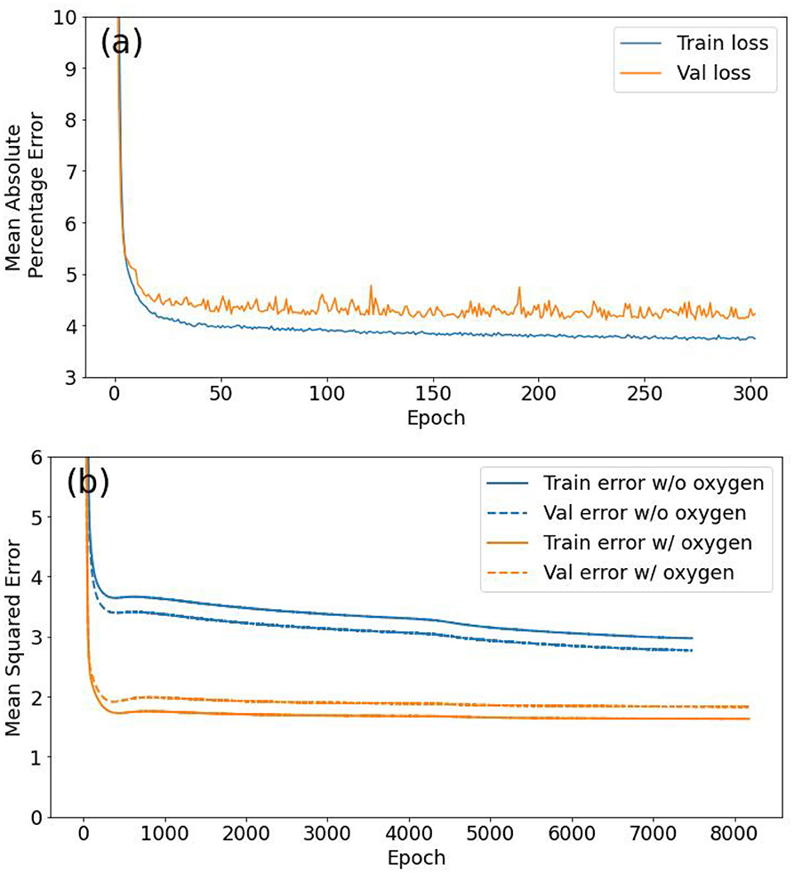
Figure 4. (a) Oxygen model training, showing the reduction of the mean absolute percentage error (loss) as a function of epochs (302 in total). Losses over both training (blue) and validation (orange) datasets are shown. (b) Comparison of training history of two different nitrate models: first without oxygen as an additional feature variable (blue lines), and second with oxygen as an extra feature (orange lines). Both the training (solid) and validation (dashed) losses are shown. An epoch is a single pass through all training examples.

The models were trained using “early-stopping,” meaning the training was stopped when the validation dataset error flattened out for 50 epochs, where an epoch is one pass through all training examples. All features for all models were standardized by subtracting the mean and dividing by the standard deviation before training so all features carried equal emphasis for the models.

Finally, the loss metric used to train the models also influences the predictions. Since we are primarily interested in reducing the mean absolute percentage error (MAPE) between the true and predicted values, we trained the models with MAPE loss. Although this resulted in good results, for oxygen, it produced misleading results for the nutrient predictions. This is because the absolute errors (true − predicted) can translate into large percentage errors for true ≈ 0 (which is the case for most nutrient observations), relative to percentage errors for larger true values. As a result, we used MSE loss for nutrient models.

The aim of the nutrient prediction models was to apply them to mooring data to create a mooring timeseries. Since no reliable dissolved oxygen data is available, we do not use oxygen as a feature variable during prediction. However, to gauge the model improvement, alternative models with oxygen as an extra feature were also trained for predicting nitrates, phosphates, and silicates. The training curves for the 6 feature and 6 + 1 feature nitrate models are shown in Figure 4b.

3.2. Results

The final test dataset mean absolute percentage error of the oxygen model was 3.97% which equates to an accuracy of 96.03%. Figures 5A,B show that most predictions fall close to the true oxygen concentration, however there are some large outliers with errors up to 60% (Figure 5B). Furthermore, the model seems to under-predict the oxygen concentrations on the higher end of the distribution, and over-predict the concentrations on the lower end (Figure 5). This is also seen in Figure 6, which shows that the range of the predicted values is smaller than that of the true Oxygen concentrations. Finally, Figure 7A shows that the large errors occur randomly throughout the temperature-salinity distribution instead of being concentrated in a particular range.

FIGURE 5

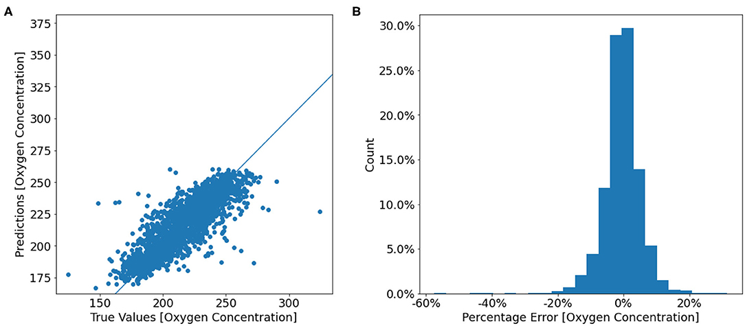
Figure 5. (A) Scatter plot of the true oxygen concentrations from the test dataset against the model predicted oxygen concentrations. (B) A histogram of the prediction error percentage [(true − predicted)/true]. Counts are displayed as a percentage of the total test data.

FIGURE 6

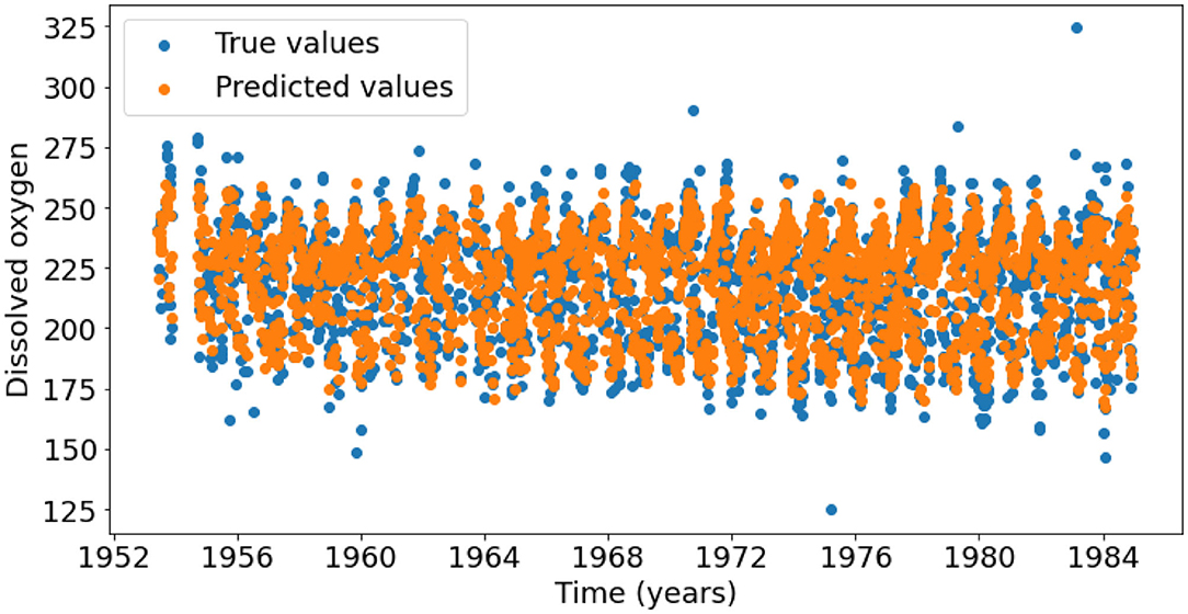
Figure 6. Timeseries of the true (blue points) and predicted (orange points) dissolved oxygen concentrations.

FIGURE 7

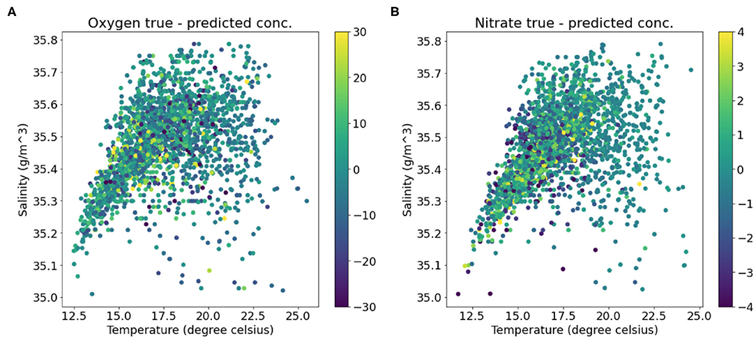
Figure 7. Temperature-Salinity diagrams colored by (A) the error in the predicted oxygen concentrations and (B) the error in the predicted nitrate concentrations.

The final mean squared error (MSE) difference between the true and predicted values over the nitrate test dataset loss is 2.63 (μmol/l)² which equates to a root mean squared error (RMSE) of 1.62 μmol l⁻¹. Two models were trained with identical model architectures and hyperparameters, however, the second model include oxygen as an additional feature variable besides the six feature variables used by the first model. The training curves for these two models are shown in Figure 4b. The model with oxygen as an extra feature had a lower loss compared to the model with the original six variables, with the final MSE (RMSE) of 1.83 (μmol/l)² (1.35 μmol l⁻¹). Temperature-Salinity diagram (Figure 7B) indicates that the large errors are located throughout the entire temperature-salinity range with the majority close to the mean of the temperature-salinity distribution (Figure 8B).

FIGURE 8

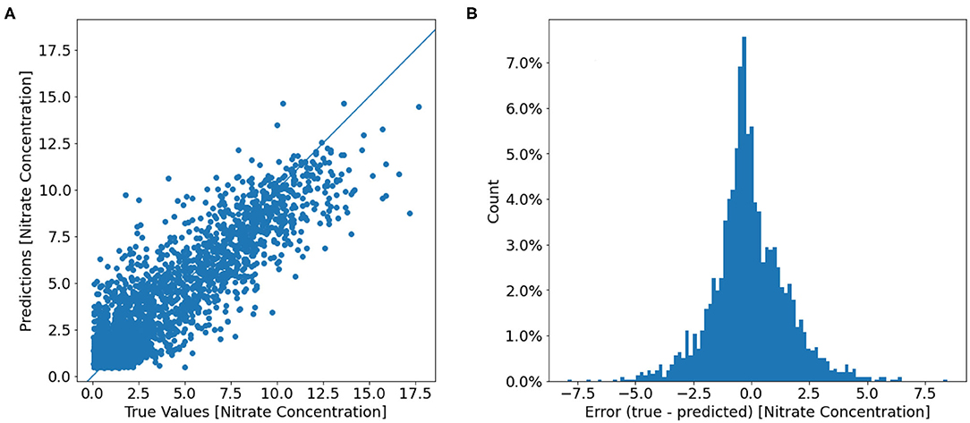
Figure 8. (A) Scatter plot of the true nitrate concentrations (μmol l⁻¹) from the test dataset against the model predicted oxygen concentrations. (B) A histogram of the prediction error [(true − predicted)]. Counts are displayed as a percentage of the total test data.

The final MSE and RMSE over the test dataset for the six feature phosphate model were 0.0099 (μmol/l)² and 0.0995 μmol l⁻¹, respectively, and for the seven feature (including oxygen) were 0.0058 (μmol/l)² and 0.0765 μmol l⁻¹, respectively. For comparison, the phosphate data ranged between 0.02 and 1.80 μmol l⁻¹. Similarly, the MSE and RMSE over the test dataset for the six feature phosphate model were 0.78 (μmol/l)² and 0.89 μmol l⁻¹, respectively, and for the seven feature (including oxygen) were 0.42 (μmol/l)² and 0.65 μmol l⁻¹, respectively. The silicate concentration ranged between 0.03 and 15.20 μmol l⁻¹.

4. Gap-Filling Timeseries

4.1. Model

Long Short-term Memory (LSTM) NNs have been used to predict (fill) gaps in temperature timeseries. These models have proved extremely effective in predicting sequence data, such as timeseries and language problems (Lipton et al., 2015). The nodes in LSTMs are enclosed within memory cells along with an input gate, an internal state, a forget gate and an output gate (see Lipton et al., 2015 for a detailed explanation). These elements inside the memory cell are connected to each other in a specific way, and also contain recurrent connections with adjacent timesteps as is typical of an RNN. It is through the inclusion of this internal state that LSTMs remember long-term information and also overcome the vanishing and exploding gradients problem (Hochreiter and Schmidhuber, 1997). LSTMs use a short past window to predict multiple timesteps into the future and average loss over all the predicted timesteps.

Three successive models were trained in order to infill gaps of different lengths. Since three out of nine gaps were <6 days long (Table 1), the first model used a history window 30 days long to fill gaps up to 6 days long. This history window length was chosen since it resulted in the lowest loss compared to history lengths of 15 and 6. To increase the number of training examples, the second model uses samples from the original timeseries and the filled gaps based on the first model to infill gaps of up to 30 days based on 30 days of history. The three gaps that ranged 6–30 days long are thus filled with model 2. The third model was trained based on training examples from the timeseries with gaps up to 30 days long filled with models 1 and 2, and was used to fill the longest remaining gaps (30–91 days long) based on 91 days of history. We avoided using history windows longer than the prediction windows for models 2 and 3, since this would reduce the number of training examples extracted from the timeseries. Furthermore, our choices of history window lengths results in high model accuracy as discussed in the results section (section 4.2). Thus, our approach is somewhat auto-regressive as predictions from previous models are used to generate training examples for the next model. Note, that such an auto-regressive approach results in compounding errors from previous models. As a result, the true model losses for models 2 and 3 could be higher than as noted in section 4.2.

We used 2,217, 2,130, and 1,793 training examples to train models 1, 2, and 3, respectively with each example consisting of the history window and the prediction window. These made up 90% of the total pairs of history and prediction windows available for each model with the remaining 10% of examples used for validation. We used a smaller percentage of examples for validation compared to the oxygen and nutrient models since we have more data available and hence fewer validation examples were necessary.

Temperature timeseries were standardized before training similar to the feature standardization for the oxygen and nutrient models as this has been shown to improve training efficiency and model convergence for LSTMs (Laurent et al., 2016). This meant that although MAPE is the metric of interest for us, it could not be used as a loss function because of the scaled temperature values close to zero. Thus, a modified MAPE loss that used the training history mean and standard deviation to reverse the standardization before calculating the MAPE was used. Similar to the co-variate modeling, the Adam optimizer with the default learning rate of 0.001 was used.

The architecture for the three models used for filling temperature gaps is described Table 3. The bidirectional layer is a wrapper that takes the layer of hidden nodes and connects them in the opposite direction so the hidden state of the first layer “remembers” information from the past while the hidden state variable of the second layer “remembers” information from the future. Thus, a bidirectional LSTM is able to learn contextual information which is important for gap-filling problems. However, since model 3 had to predict a much longer window compared to models 1 and 2, the approaches used for models 1 and 2 resulted in larger losses of around 4%. As a result, model 3 was treated as a multivariate timeseries forecasting problem where the 91 days after the gap were chronologically reversed (i.e., the vector of values for day 1, 2, 3, …, 91 after the gap became the vector of values corresponding to days 91, 90, 89, …, 1 after the gap) and given to the model as another feature variable. This way contextual information was more explicitly encoded into the “multi-variate” model and the resulting losses were lower.

TABLE 3

Table 3. Description of the four layer model architecture used to fill temperature gaps.

To assess the uncertainty of the long window predictions, we include dropout in each LSTM layer. Dropout is a regularization technique where a given percentage of nodes are randomly turned of during each training step to reduce model overfitting. Traditionally no dropout is included during the evaluation stage. However, it has recently been shown that predictions with dropout act as monte carlo estimates and represent Bayesian approximations (Gal and Ghahramani, 2016b). Such dropout based uncertainty is much less computationally expensive compared to fully Bayesian approaches, such as Bayesian NNs. In LSTMs dropout is typically applied to the input and recurrent connections as opposed to the nodes themselves (Gal and Ghahramani, 2016a). We drop 25% of input and recurrent connection randomly in model 3. We apply dropout only to model 3 as a demonstration of deriving modeling uncertainty using NNs.

Similar to the oxygen and nutrient models, the training was automatically stopped when there was no improvement in validation loss for 20 epochs. The performance of model 1 was compared with three other models; a single layer model with 64 nodes, a single layer model with 128 nodes, and finally a model with the same three layer architecture as model 1, except without the bidirectional layers. All three alternative models were trained with the same training data as model 1, however, the final losses in all three cases were worse than the original model 1. Furthermore, there was no noticeable differences between the single layer model with 64 nodes and the single layer model with 128 nodes. Figure 9 shows the training history of the final three models trained for the short, medium and long gaps.

FIGURE 9

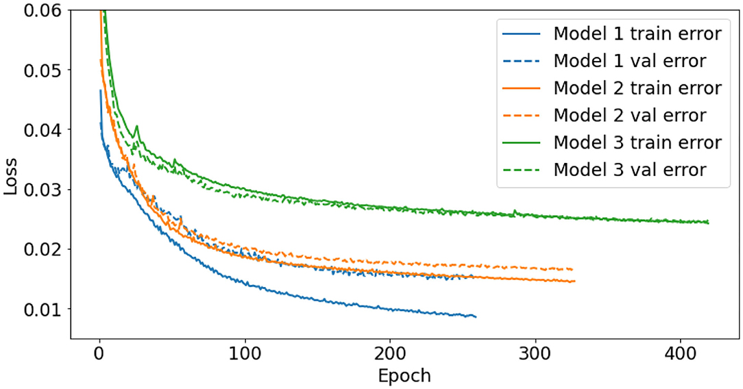
Figure 9. Training history of the three models used to fill temperature gaps. Model 1 (blue) fills gaps up to 6 days long, model 2 (orange) fills fill gaps 6–30 days long, and model 3 (green) fills the remaining 2 gaps, 79 and 91 days long. Both the training (solid) and validation (dashed) losses are shown. An epoch is a single pass through all training examples.

4.2. Results

Sample predictions from model 1, 2, and 3 reveal that the models predict the general shape of the true observations well-based on 30, 30, and 91 days of history, respectively, but lose progressively more day-to-day variability as the prediction window lengthens (6, 30, and 91, respectively) (Figure 10). Although Figure 10 only shows a single example from the test dataset for each model, similar behavior is observed for other examples as well. Overall, however, the models (1, 2, and 3) perform well with the final validation dataset losses of only 1.53, 1.65, and 2.42%, respectively (resulting in accuracies of 98.47, 98.35, and 97.58%, respectively). Note that the validation loss was calculated by averaging the differences between the true and predicted values over all days of the prediction window of the validation examples.

FIGURE 10

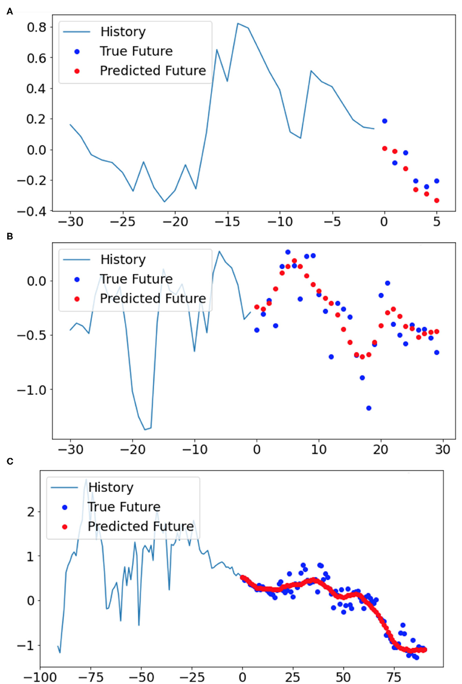
Figure 10. Three samples of the model filled gaps from the validation dataset based on (A) model 1, (B) model 2, and (C) model 3, respectively. The blue lines show the 30, 30, and 90-day history timeseries (normalized units) which were used as input for the LSTM models 1, 2, and 3, respectively. The blue points demonstrate the observed temperatures whereas the red points indicate the model predicted temperatures over the next (A) 6, (B) 30, and (C) 91 days after the history window.

The NN predictions of the largest gaps contain much less variability when compared to the temperature observations before and after Figure 11. A hundred monte carlo dropout estimates are shown in Figure 11. The prediction from model 3 without any dropout is approximately in the middle of the Monte Carlo estimates which is reasonable since it can be thought of as averaging a hundred different model architectures (Hinton et al., 2012).

FIGURE 11

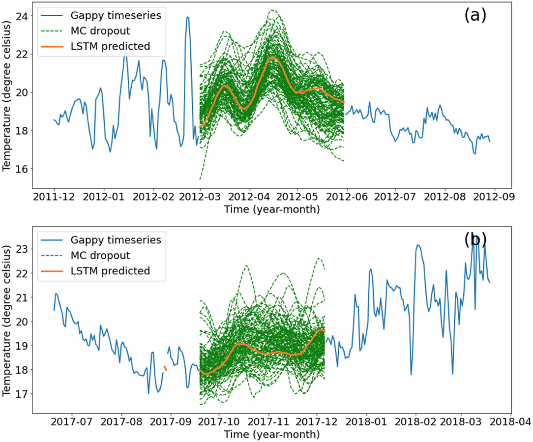
Figure 11. Gap-filling of the (a) 91 day gap and (b) 79 day gap based on the final LSTM model (orange) and the five models with dropout layers (where 40% of nodes in each of the three layers are randomly switched off in the training process) in green, representing model uncertainty. Original timeseries is shown in blue. Units: °C.

The entire timeseries from 2011 to 2018 (Figure 3) was filled using predictions from the three chosen LSTM models and is shown in Figure 12. The linear interpolation does not preserve any of the seasonal or shorter timescale variability that the NN prediction does, however, as mentioned earlier the NNs struggle to reproduce even shorter timescale variability present in the observations. At first glance the jumps between the filled gaps and the original data may not seem smooth in some cases (e.g., the last gap in 2013, Figure 12B). However, in all cases the jumps at the start or end of the gaps are similar to the day to day variability in the vicinity of the gaps.

FIGURE 12

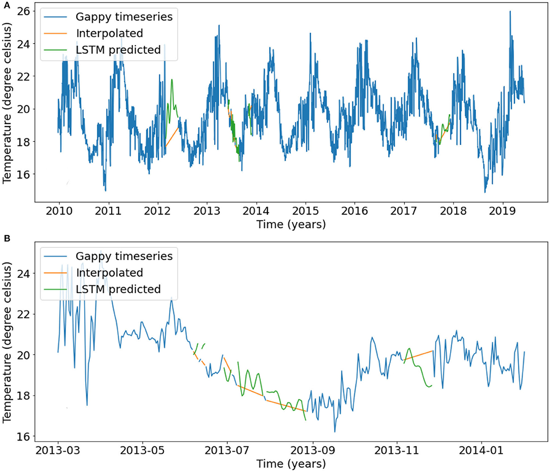
Figure 12. (A) The final filled temperature timeseries at the 24.5 m bin of the Port Hacking mooring. Blue line represents the original timeseries with gaps, green lines represent the predictions from the LSTM models and the orange lines represent the predictions from linear interpolation. The long 2012 and 2017 gaps were filled using the 91-day model 3, the gaps longer than 6 days were filled using the 30 day model 2, and the remaining gaps were filled using model 1. (B) Same as (A) but zoomed in on the series of gaps in 2013.

5. Discussion

A simple artificial neural network was shown to fit oxygen data with a high degree of accuracy. The model contained three hidden layers with 64, 64, and 8 nodes, respectively and was able to achieve accuracy of over 96%. Although most predictions were comfortably close to the true values, a small number of predictions presented large biases. Figure 6 indicates that the predicted values struggles to predict some extreme concentrations. This is further confirmed by Figure 5A that shows that the distribution of true to predicted oxygen concentrations is wide rather than tall, meaning the NN model is predicting concentrations in the 170–260 μmol l⁻¹ range even though the true values are outside this range. Note that, some of these true extreme concentrations may be a result of stochastic variability or due to variance that cannot be explained based on the chosen variables.

Sauzède et al. (2017) has also developed feedforward NN models with three layers called CANYON to predict subsurface nutrient concentration using the GLODAPv2 database (Olsen et al., 2016) that contains data from 37,863 stations globally. The CANYON models predict nutrients from latitude, longitude, DOY, year, pressure, temperature, salinity, and oxygen as features using a two hidden layer NN. Our nutrient models compare well with the CANYON models. The nitrate model RMSE with and without oxygen as a feature are 1.35 and 1.62 μmol l⁻¹ compared to 0.93 μmol l⁻¹ for CANYON. The phosphate model RMSE with and without oxygen as a feature are 0.077 and 0.010 μmol l⁻¹ compared to 0.066 μmol l⁻¹ for CANYON. Finally, the silicate model RMSE with and without oxygen as a feature are 0.65 and 0.89 μmol l⁻¹ compared to 3.0 μmol l⁻¹ for CANYON. Note, that the GLODAPv2 silicate values are much larger, in the range of 0–200 μmol l⁻¹, compared to the range of values used here (0–10 μmol l⁻¹) likely due to the depth of the samples in the water column. We suggest that the slightly lower RMSE obtained using CANYON to predict nitrate and phosphate can be explained by the significantly larger dataset used by Sauzède et al. (2017). Furthermore, our largest errors are comparable if not smaller than the CANYON models. Finally, we note that, unlike the CANYON models, our models have successfully learned to not predict concentrations below zero (Figure 8A). The CANYON models are based on stations located in varying regions globally including regional coastal and open ocean sites making them much more generalized than the models presented in this study. This means that the results presented here, while not fully comparable do provide some indication of the suitable performance of our models.

The oxygen data distribution is unbounded and symmetric about its mean, whereas the distributions of the nutrients are bounded by zero and skewed with most observations close to zero. Since MAPE is defined as (true − predicted)/true × 100, when the true distribution is dominated by true value close to zero (<1), the errors for these values carry much greater importance than larger true values. This means that models that use MAPE as a loss can artificially decrease their final mean loss by paying more attention to training examples which correspond to true values (labels) close to zero. This can be seen in Supplementary Figure 1, which shows the error distribution using a NN model with MAPE loss is skewed toward the right compared to Figure 8. A similar issue was encountered with the timeseries gap-filling models where the output variables needed to be standardized rendering them unsuitable to be trained with MAPE loss. In this case, we ended up implementing a modified MAPE loss that removed the standardization by multiplying by the training dataset standard deviation and adding the training dataset mean. Thus, the metric used to calculate loss proved pivotal when training the nutrient and temperature gap-filling models.

The training variance (difference between the training and validation error) for the temperature timeseries gap-filling models decreases with longer observations (Figure 9). However, for the purposes of a long, continuous, filled timeseries, such as creating climatologies or calculating trends, i.e., calculating long-term average statistics, short gaps are less influential on the result compared to the long gaps. Hence, the higher overfitting in model 1 compared to models 2 and 3 is less concerning. An explanation for the higher training variance of model 1 could be that models 2 and 3, which predict longer windows, learn the underlying long-term variability better than model 1, and do not learn the stochastic variability which is specific to the training dataset.

Although the predicted sequences based on the validation examples look plausible, it seems impractical to gap-fill with prediction from a single model without uncertainty estimates. There are two sources of uncertainty here: the dataset uncertainty or sampling uncertainty/bias and the modeling uncertainty. As demonstrated, dropout in hidden layers can account for the modeling uncertainty. Gal and Ghahramani (2016b) showed that such a dropout based approach can act as a Bayesian approximation of a Gaussian process, thus making it unnecessary to use Bayesian NN (Blundell et al., 2015) which can be difficult to train and computationally expensive [e.g., CANYON-B (Bittig et al., 2018)]. Furthermore, dropout in the input layers can also account for dataset uncertainty (especially useful when training on small datasets) (Hinton et al., 2012).

Since the oxygen model fails to predict some extremes (Figure 6) and the temperature gap-filling model predictions resemble smoothed estimates (Figure 10), some smoothing is apparent in NN predictions. Depending on the use case this might be worth keeping in mind. For example, our predictions are still useful for estimating long term variability.

Since ocean observing has evolved significantly over the past century, so have the ocean observing practices. It is not possible to train a neural network to use the long term, low frequency bottle data alongside shorter record, higher frequency data, such as from satellites and moorings. Hence it is not possible to train a single model that takes advantage of all the data. Furthermore, the size of the bottle dataset used for the nitrate and oxygen concentration modeling is limited by its manual collection. It has a nominal collection frequency of 2 weeks but, due to the manual nature of the data collection, sampling frequency varies greatly, with gaps up to a few months at times. Additionally, there are a lot more observations at certain depths compared to others. Automated sampling can also create consistent observations at all depths. This emphasizes the requirement for automated instruments that can collect data at regular intervals and at high frequencies, and hence has implications for ocean observing system design.

6. Conclusions

The application of neural network models was demonstrated on typical oceanographic datasets using off-the-shelf programming libraries. Point based observations at a single location (Port Hacking, Australia) were used to accurately model oxygen, nutrients, and temperatures. The oxygen model loss was below 4% resulting in an accuracy of over 96%. The nitrate, phosphate and silicate RMSE were 1.62, 0.0995, and 0.89 μmol l⁻¹, respectively. Finally, the temperature gap-filling model losses were 1.53, 1.65, and 2.42%, respectively (resulting in accuracies of 98.47, 98.35, and 97.58%, respectively).

Such NN based approaches have the advantage of being computationally inexpensive to both train and run. The models can be used to generate realtime predictions suitable for web-based data visualization and outreach. Furthermore, all modeling in this study was done with popular, open source, off-the-shelf frameworks, allowing easy implementation by non-experts. To further facilitate the uptake of NN modeling in oceanography, we provided details on the training process and the architectural design of the NN used in the context of fit-for-purpose modeling throughout this study.

The models developed in this study are site specific and likely do not generalize to other ocean regions, however our results do provide suitable proof of concept. Unfortunately, due to the limited data the nutrient models do not yet perform well-enough to be used as a virtual sensor or as a replacement for in situ sampling. As such future work will include training the oxygen and nutrient models at other locations where long-term observations are available to see if the models generalize and/or are able to improve their predictive skill.

The temperature gap-filling procedure can be applied at all depths to create a suite of temperature products. However, distinct univariate models for each depth may not preserve the correlation between adjacent temperature sensors. This could potentially be helped by training multivariate models that employ correlated sensors above and below the desired depth as additional feature variables based on our multivariate gap-filling approach. Our approach paves the way to create a whole suite of data products using the long term IMOS data.

Data Availability Statement

The datasets presented in this study can be found in online repositories. The names of the repository/repositories and accession number(s) can be found at: https://catalogue-imos.aodn.org.au/geonetwork/srv/eng/catalog.search#/metadata/fa93c66e-0e56-7e1d-e043-08114f8c1b76, https://catalogue-imos.aodn.org.au/geonetwork/srv/eng/catalog.search#/metadata/7e13b5f3-4a70-4e31-9e95-335efa491c5c.

Author Contributions

SC and MR conceived the study and wrote the manuscript. MR led the data collection. SC conducted the analysis.

Funding

SC was partially funded by UNSW Australia as a co-investment to IMOS and an Australian Research Council Linkage Project #LP170100498 to MR. This research includes computations using the computational cluster Katana supported by Research Technology Services at UNSW Sydney.

Conflict of Interest

The authors declare that the research was conducted in the absence of any commercial or financial relationships that could be construed as a potential conflict of interest.

Acknowledgments

Data was sourced from Australia's Integrated Marine Observing System (IMOS)–IMOS was enabled by the National Collaborative Research Infrastructure Strategy (NCRIS). It was operated by a consortium of institutions as an unincorporated joint venture, with the University of Tasmania as Lead Agent.

Supplementary Material

The Supplementary Material for this article can be found online at: https://www.frontiersin.org/articles/10.3389/fmars.2021.637759/full#supplementary-material

References

Abadi, M., Barham, P., Chen, J., Chen, Z., Davis, A., Dean, J., et al. (2016). “Tensorflow: a system for large-scale machine learning,” in 12th USENIX Symposium on Operating Systems Design and Implementation (OSDI 16) (Savannah, GA), Vol. 101, 265–283.

Google Scholar

Adikane, H. V., Singh, R. K., Thakar, D. M., and Nene, S. N. (2001). Single-step purification and immobilization of penicillin acylase using hydrophobic ligands. Appl. Biochem. Biotechnol. 94, 127–134. doi: 10.1385/ABAB:94:2:127

PubMed Abstract | CrossRef Full Text | Google Scholar

Ashok, K., Behera, S. K., Rao, S. A., Weng, H., and Yamagata, T. (2007). El Niño Modoki and its possible teleconnection. J. Geophys. Res. Oceans 112, 1–27. doi: 10.1029/2006JC003798

CrossRef Full Text | Google Scholar

Bailey, K., Steinberg, C., Davies, C., Galibert, G., Hidas, M., McManus, M. A., et al. (2019). Coastal Mooring observing networks and their data products: recommendations for the next decade. Front. Mar. Sci. 6:180. doi: 10.3389/fmars.2019.00180

CrossRef Full Text | Google Scholar

Bittig, H. C., Steinhoff, T., Claustre, H., Fiedler, B., Williams, N. L., Sauzède, R., et al. (2018). An alternative to static climatologies: robust estimation of open ocean CO2 variables and nutrient concentrations from T, S, and O₂ data using bayesian neural networks. Front. Mar. Sci. 5:328. doi: 10.3389/fmars.2018.00328

CrossRef Full Text | Google Scholar

Blundell, C., Cornebise, J., Kavukcuoglu, K., and Wierstra, D. (2015). Weight uncertainty in neural networks. arXiv [Preprint]. arXiv:1505.05424.

Google Scholar

Bolton, T., and Zanna, L. (2019). Applications of deep learning to ocean data inference and subgrid parameterization. J. Adv. Model. Earth Syst. 11, 376–399. doi: 10.1029/2018MS001472

CrossRef Full Text | Google Scholar

Emmert-Streib, F., Yang, Z., Feng, H., Tripathi, S., and Dehmer, M. (2020). An introductory review of deep learning for prediction models with big data. Front. Artif. Intell. 3:4. doi: 10.3389/frai.2020.00004

PubMed Abstract | CrossRef Full Text | Google Scholar

Fourrier, M., Coppola, L., Claustre, H., D'Ortenzio, F., Sauzède, R., and Gattuso, J. P. (2020). A regional neural network approach to estimate water-column nutrient concentrations and carbonate system variables in the Mediterranean sea: CANYON-MED. Front. Mar. Sci. 7:620. doi: 10.3389/fmars.2020.00620

CrossRef Full Text | Google Scholar

Gal, Y., and Ghahramani, Z. (2016a). “A theoretically grounded application of dropout in recurrent neural networks,” in Advances in Neural Information Processing Systems, eds D. Lee, M. Sugiyama, U. Luxburg, I. Guyon, and R. Garnett (Barcelona: Barcelona NIPS), 1027–1035. Available online at: https://proceedings.neurips.cc/paper/2016

Gal, Y., and Ghahramani, Z. (2016b). “Dropout as a bayesian approximation: representing model uncertainty in deep learning,” in International Conference on Machine Learning, 1050–1059.

Google Scholar

Graves, A. (2013). Generating Sequences With Recurrent Neural Networks. arXiv [Preprint]. arXiv:1308.0850.

Google Scholar

Han, G., and Shi, Y. (2008). Development of an Atlantic Canadian coastal water level neural network model. J. Atmos. Ocean. Technol. 25, 2117–2132. doi: 10.1175/2008JTECHO569.1

CrossRef Full Text | Google Scholar

Han, M., Feng, Y., Zhao, X., Sun, C., Hong, F., and Liu, C. (2019). A convolutional neural network using surface data to predict subsurface temperatures in the Pacific Ocean. IEEE Access 7, 172816–172829. doi: 10.1109/ACCESS.2019.2955957

CrossRef Full Text | Google Scholar

Hemming, M. P., Roughan, M., and Schaeffer, A. (2020). Daily subsurface ocean temperature climatology using multiple data sources: new methodology. Front. Mar. Sci. 7:485. doi: 10.3389/fmars.2020.00485

CrossRef Full Text | Google Scholar

Hinton, G. E., Osindero, S., and Teh, Y.-W. (2006). A fast learning algorithm for deep belief nets. Neural Comput. 18, 1527–1554. doi: 10.1162/neco.2006.18.7.1527

PubMed Abstract | CrossRef Full Text | Google Scholar

Hinton, G. E., Srivastava, N., Krizhevsky, A., Sutskever, I., and Salakhutdinov, R. R. (2012). Improving Neural Networks by Preventing Co-Adaptation of Feature Detectors. arXiv [Preprint]. arXiv:1207.0580.

Google Scholar

Hochreiter, S., and Schmidhuber, J. (1997). Long short-term memory. Neural Comput. 9, 1735–1780. doi: 10.1162/neco.1997.9.8.1735

CrossRef Full Text | Google Scholar

Hsieh, W. W. (2009). Machine Learning Methods in the Environmental Sciences: Neural Networks and Kernels. New York, NY: Cambridge University Press.

Google Scholar

Ingleton, T., Morris, B., Pender, L., Darby, I., Austin, T., and Galibert, G. (2014). Standardised Profiling CTD Data Processing Procedures V2.0. Technical Report March, Australian National Mooring Network.

Ketkar, N. (2017). “Stochastic gradient descent BT–deep learning with python: a hands-on introduction,” in Deep Learning With Python, ed N. Ketkar (Berkeley, CA: Apress), 113–132. doi: 10.1007/978-1-4842-2766-4_8

CrossRef Full Text | Google Scholar

Kingma, D. P., and Ba, J. L. (2015). “Adam: a method for stochastic optimization,” in 3rd International Conference on Learning Representations, ICLR 2015–Conference Track Proceedings (San Diego, CA), 1–15.

Google Scholar

Krasnopolsky, V. M. (2013). The application of neural networks in the earth system sciences. Neural Networks Emulations for Complex Multidimensional Mappings. Dordrecht: Springer.

Google Scholar

Krogh, A., and Hertz, J. A. (1992). “A simple weight decay can improve generalization,” in Advances in Neural Information Processing Systems, Vol. 517, eds J. Moody, S. Hanson, and R. P. Lippmann (Denver, CO: Denver NIPS), 4698. Available online at: https://proceedings.neurips.cc/paper/1991

Google Scholar

Kwon, B. C., Choi, M. J., Kim, J. T., Choi, E., Kim, Y. B., Kwon, S., et al. (2019). RetainVis: visual analytics with interpretable and interactive recurrent neural networks on electronic medical records. IEEE Trans. Vis. Comput. Graph. 25, 299–309. doi: 10.1109/TVCG.2018.2865027

PubMed Abstract | CrossRef Full Text | Google Scholar

Laurent, C., Pereyra, G., Brakel, P., Zhang, Y., and Bengio, Y. (2016). “Batch normalized recurrent neural networks,” in ICASSP, IEEE International Conference on Acoustics, Speech and Signal Processing–Proceedings (Shanghai), 2657–2661. doi: 10.1109/ICASSP.2016.7472159

CrossRef Full Text | Google Scholar

LeCun, Y., Bengio, Y., and Hinton, G. (2015). Deep learning. Nature 521, 436–444. doi: 10.1038/nature14539

CrossRef Full Text | Google Scholar

Lee, K. A., Roughan, M., Malcolm, H. A., and Otway, N. M. (2018). Assessing the use of area- and time-averaging based on known de-correlation scales to provide satellite derived sea surface temperatures in coastal areas. Front. Mar. Sci. 5:261. doi: 10.3389/fmars.2018.00261

CrossRef Full Text | Google Scholar

Lee, K. A., Smoothey, A. F., Harcourt, R. G., Roughan, M., Butcher, P. A., and Peddemors, V. M. (2019). Environmental drivers of abundance and residency of a large migratory shark, Carcharhinus leucas, inshore of a dynamic western boundary current. Mar. Ecol. Prog. Ser. 622, 121–137. doi: 10.3354/meps13052

CrossRef Full Text | Google Scholar

Lguensat, R., Sun, M., Fablet, R., Tandeo, P., Mason, E., and Chen, G. (2018). “EddyNet: a deep neural network for pixel-wise classification of oceanic eddies,” in IGARSS 2018–2018 IEEE International Geoscience and Remote Sensing Symposium (Valencia), 1764–1767. doi: 10.1109/IGARSS.2018.8518411

CrossRef Full Text | Google Scholar

Lipton, Z. C., Berkowitz, J., and Elkan, C. (2015). A Critical Review of Recurrent Neural Networks for Sequence Learning. arXiv [Preprint]. arXiv:1506.00019

Google Scholar

Lu, W., Su, H., Yang, X., and Yan, X. H. (2019). Subsurface temperature estimation from remote sensing data using a clustering-neural network method. Rem. Sens. Environ. 229, 213–222. doi: 10.1016/j.rse.2019.04.009

CrossRef Full Text | Google Scholar

Lundberg, S. M., and Lee, S. I. (2017). “A unified approach to interpreting model predictions,” in Advances in Neural Information Processing Systems, eds I. Guyon, U. V. Luxburg, S. Bengio, H. Wallach, R. Fergus, S. Vishwanathan, and R. Garnett (Long Beach, CA: Long Beach NIPS), 4766–4775. Available online at: https://proceedings.neurips.cc/paper/2017

Google Scholar

Lynch, T. P., Morello, E. B., Evans, K., Richardson, A. J., Rochester, W., Steinberg, C. R., et al. (2014). IMOS national reference stations: a continental-wide physical, chemical and biological coastal observing system. PLoS ONE 9:e0113652. doi: 10.1371/journal.pone.0113652

PubMed Abstract | CrossRef Full Text | Google Scholar

Makarynskyy, O. (2005). Artificial neural networks for wave tracking, retrieval and prediction. Pacific Oceanogr. 3, 21–30.

Google Scholar

Makarynskyy, O., Makarynska, D., Kuhn, M., and Featherstone, W. E. (2004). “Using artificial neural networks to estimate sea level in continental and island coastal environments,” in Hydrodynamics IV: Theory and Applications, ed Y. Goda (Yokohama: Yokohama ICHD), 451–457. doi: 10.1201/b16815-66

CrossRef Full Text | Google Scholar

Malan, N., Roughan, M., and Kerry, C. (2020). The rate of coastal temperature rise adjacent to a warming western boundary current is nonuniform with latitude. Geophys. Res. Lett. 48:e2020GL090751. doi: 10.1029/2020GL090751

CrossRef Full Text | Google Scholar

Morello, E. B., Galibert, G., Smith, D., Ridgway, K. R., Howell, B., Slawinski, D., et al. (2014). Quality Control (QC) procedures for Australia's National Reference Station's sensor data–comparing semi-autonomous systems to an expert oceanographer. Methods Oceanogr. 9, 17–33. doi: 10.1016/j.mio.2014.09.001

CrossRef Full Text | Google Scholar

Nair, V., and Hinton, G. E. (2010). “Rectified linear units improve restricted Boltzmann machines,” in ICML (Haifa).

Google Scholar

Oehmcke, S., Zielinski, O., and Kramer, O. (2018). Input quality aware convolutional LSTM networks for virtual marine sensors. Neurocomputing 275, 2603–2615. doi: 10.1016/j.neucom.2017.11.027

CrossRef Full Text | Google Scholar

Olsen, A., Key, R. M., Van Heuven, S., Lauvset, S. K., Velo, A., Lin, X., et al. (2016). The global ocean data analysis project version 2 (GLODAPv2)–an internally consistent data product for the world ocean. Earth Syst. Sci. Data 8, 297–323. doi: 10.5194/essd-8-297-2016

CrossRef Full Text | Google Scholar

Rawat, W., and Wang, Z. (2017). Deep convolutional neural networks for image classification: a comprehensive review. Neural Comput. 29, 2352–2449. doi: 10.1162/neco_a_00990

PubMed Abstract | CrossRef Full Text | Google Scholar

Rosenblatt, F. (1957). The Perceptron–A Perceiving and Recognizing Automaton. New York, NY: Cornell Aeronautical Laboratory.

Google Scholar

Rosindell, J., and Wong, Y. (2018). “Biodiversity, the tree of life, and science communication,” in Phylogenetic Diversity: Applications and Challenges in Biodiversity Science, eds Rosa Scherson and D. Faith (New York, NY: Springer International publishing), 41–71. doi: 10.1007/978-3-319-93145-6_3

CrossRef Full Text | Google Scholar

Roughan, M., Morris, B. D., and Suthers, I. M. (2010). NSW-IMOS: an integrated marine observing system for Southeastern Australia. IOP Conf. Ser. Earth Environ. Sci. 11:12030. doi: 10.1088/1755-1315/11/1/012030

CrossRef Full Text | Google Scholar

Roughan, M., Schaeffer, A., and Kioroglou, S. (2013). “Assessing the design of the NSW-IMOS moored observation array from 2008–2013: recommendations for the future,” in 2013 OCEANS (San Diego, CA), 1–7.

Google Scholar

Roughan, M., Schaeffer, A., and Suthers, I. M. (2015). “Sustained ocean observing along the coast of southeastern australia: NSW-IMOS 2007–2014,” in Coastal Ocean Observing Systems, eds Y. Liu, H. Kerkering, and R. H. B. T. Weisberg (Boston, MA: Academic Press), 76–98. doi: 10.1016/B978-0-12-802022-7.00006-7

CrossRef Full Text | Google Scholar

Ruder, S. (2016). An Overview of Gradient Descent Optimization Algorithms. arXiv [Preprint]. arXiv:1609.04747.

Google Scholar

Sauzède, R., Bittig, H. C., Claustre, H., Pasqueron de Fommervault, O., Gattuso, J.-P., Legendre, L., et al. (2017). Estimates of water-column nutrient concentrations and carbonate system parameters in the global ocean: a novel approach based on neural networks. Front. Mar. Sci. 4:128. doi: 10.3389/fmars.2017.00128

CrossRef Full Text | Google Scholar

Schaeffer, A., and Roughan, M. (2017). Subsurface intensification of marine heatwaves off southeastern Australia: the role of stratification and local winds. Geophys. Res. Lett. 44, 5025–5033. doi: 10.1002/2017GL073714

CrossRef Full Text | Google Scholar

Schlegel, R. W., Oliver, E. C. J., Hobday, A. J., and Smit, A. J. (2019). Detecting marine heatwaves with sub-optimal data. Front. Mar. Sci. 6:737. doi: 10.3389/fmars.2019.00737

CrossRef Full Text | Google Scholar

Schmidhuber, J. (2015). Deep learning in neural networks: an overview. Neural Netw. 61, 85–117. doi: 10.1016/j.neunet.2014.09.003

PubMed Abstract | CrossRef Full Text | Google Scholar

Su, H., Li, W., and Yan, X. H. H. (2018). Retrieving temperature anomaly in the global subsurface and deeper ocean from satellite observations. J. Geophys. Res. Oceans 123, 399–410. doi: 10.1002/2017JC013631

CrossRef Full Text | Google Scholar

Sutherland, M., Ingleton, T., and Morris, B. (2017). Pre-Run Check and Field Sampling CTD Procedural Guide v. 3.0. Technical Report August, Coasts and Marine Team, New South Wales Office of Environment and Heritage, Sydney and Sydney Institute of Marine Science, Sydney, NSW.

Google Scholar

Tang, Y., and Hsieh, W. W. (2003). Nonlinear modes of decadal and interannual variability of the subsurface thermal structure in the Pacific Ocean. J. Geophys. Res. Oceans 108, 1–12. doi: 10.1029/2001JC001236

CrossRef Full Text | Google Scholar

Tangang, F. T., Hsieh, W. W., and Tang, B. (1997). Forecasting the equatorial Pacific sea surface temperatures by neural network models. Clim. Dyn. 13, 135–147. doi: 10.1007/s003820050156

CrossRef Full Text | Google Scholar

Tolman, H. L., Krasnopolsky, V. M., and Chalikov, D. V. (2005). Neural network approximations for nonlinear interactions in wind wave spectra: direct mapping for wind seas in deep water. Ocean Modell. 8, 253–278. doi: 10.1016/j.ocemod.2003.12.008

CrossRef Full Text | Google Scholar

UNESCO (2019). United Nations Decade of Ocean Science For Sustainable Development. UNESCO. Available online at: https://www.oceandecade.org/ (accessed March 03, 2021).

Google Scholar

Wynn, T. A., and Wickwar, V. B. (2007). “The effects of large data gaps on estimating linear trend in autocorrelated data,” in Annual Fellowship Symposium of the Rocky Mountain NASA Space Grant Consortium (Salt Lake City, UT).

Google Scholar

Young, T., Hazarika, D., Poria, S., and Cambria, E. (2018). Recent trends in deep learning based natural language processing. IEEE Comput. Intell. Mag. 13, 55–75. doi: 10.1109/MCI.2018.2840738

CrossRef Full Text | Google Scholar