argoFloats: An R Package for Analyzing Argo Data

An R package named argoFloats has been developed to facilitate identifying, downloading, caching, and analyzing oceanographic data collected by Argo profiling floats. The analysis phase benefits from close connections between argoFloats and the oce package, which is likely to be familiar to those who already use R for the analysis of oceanographic data of other kinds. This paper outlines how to use argoFloats to accomplish some everyday tasks that are particular to Argo data, ranging from downloading data and finding subsets to handling quality control and producing a variety of diagnostic plots. The benefits of the R environment are sketched in the examples, and also in some notes on the future of the argoFloats package.

1. The Argo Program

The ocean is not a uniform, static fluid. Rather, its properties vary with both space and time, and these variations are important not just for the ocean itself, but also for ocean-atmosphere interactions. For this reason, measuring variations of seawater properties and currents is a critical prerequisite to understanding and predicting the ocean and its place in the climate system.

Sampling the ocean with ships has proved to be somewhat problematic. Despite the high accuracy of ship-based measurements, the spatial and temporal coverage is limited, with large areas remaining unexamined for decades at a time. At particular isolated locations, the temporal issue is addressed well by moorings. However, traditional moorings provide no data until they are recovered, and so moorings are of little utility in data-assimilative modeling efforts. Satellite imagery provides another alternative to ships, providing good geographical and temporal resolution. However, sensors aboard satellites provide information mainly about surface properties, yielding little direct information about the underlying waters.

These and other limitations of ships, moorings, and satellites have been addressed by the Argo Program of drifting profiling floats, which was initiated in 1999 (see e.g., Roemmich et al., 2009). Argo floats can control their depth by altering their buoyancy, and this is key to their utility. The usual protocol is for a float to remain at a parking depth that is 1 km below the surface (or less, depending on water depth) for approximately 9 days. Then the buoyancy is reduced so that the float descends to 2 km (water depth permitting), after which buoyancy is increased, causing the float to ascend to the surface. The drift-profile pairs are a component of what are called “cycles” in Argo nomenclature.

Argo floats are typically deployed from ships and thereafter drift freely for about 4 years (Carval et al., 2019), making approximately 150 ocean profiles. During those profiles, instruments record pressure, temperature, and electrical conductivity (through which salinity is computed), with the optional addition of other quantities to be described below. These data, along with location inferred by GPS, are transmitted by the Argos, Iridium, or Orbcomm communication systems to receiving stations (Schmid et al., 2007). (Other, less precise, positioning systems were used in past years.) Thus, Argo floats provide profiling data at the transmitting sites, and an analysis of those site locations permits inferences about currents at the parking depths (Ollitrault et al., 2013).

The original Argo Program (now called the “Core” Program) was extended to address the evolving needs of the research community, forming what is now known as the biogeochemical (“BGC”) Argo Program, which began by deploying optical and oxygen sensors on Argo floats (Roemmich et al., 2019). Today, BGC-Argo floats may carry additional sensors including oxygen, pH, nitrate, downward irradiance, chlorophyll fluorescence, and optical backscattering (Bittig et al., 2019), providing insight about biogeochemical processes in the upper 2 km of the ocean. The BGC initiative was then followed by the “Deep” Argo Program, with floats descending as far as 6 km below the surface, starting with a pilot phase in 2014 (Gasparin et al., 2020). As Figure 1 shows, there has been a marked increase in Argo sampling since the onset of the program, with a plateau in recent years. As of November 2020, over 16000 Core Argo floats had been deployed, along with over 1400 BGC floats and over 100 Deep floats (see Argo (2020) for notes on data availability).

FIGURE 1

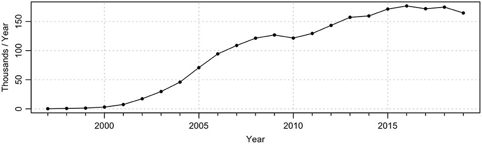
Figure 1. Number of Argo cycles executed annually, revealing an early steep rise followed by a plateau in recent years.

By virtue of the large number of floats and the short time between their profiles, the Argo Program provides a valuable supplement to traditional ship-based Conductivity Temperature Depth (“CTD”) instruments. In 2018, for example, there were 8 times as many Argo profiles as there were ship-based CTD profiles recorded in the World Ocean Database (see Boyer et al. (2018) for an introduction to this database). However, this is an underestimate of the significance of the Argo Program, because the ship-based CTD profiles tend to be acquired only in selected regions. This is illustrated in Figure 2, which reveals dense Argo sampling in large expanses of the ocean that received little ship coverage. (Although the Arctic is presently sampled poorly by both methods, efforts are underway to develop Argo floats suitable for the Arctic; see e.g., Nguyen et al. (2020) for a discussion.)

FIGURE 2

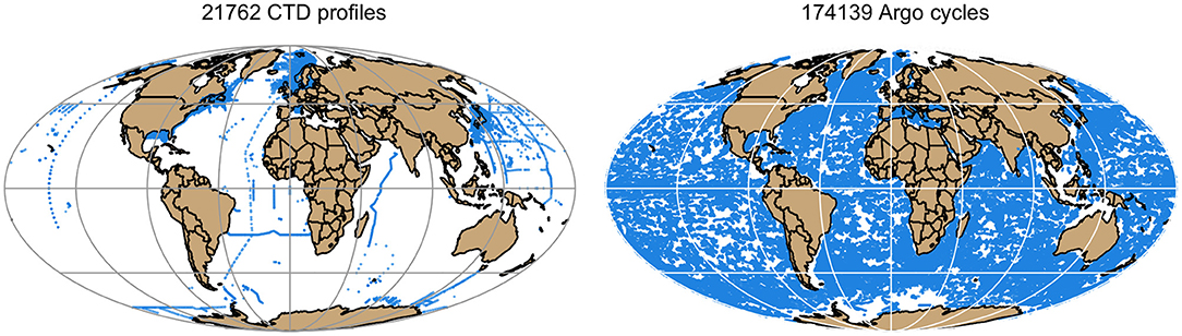
Figure 2. Comparison of spatial sampling during the year 2018 using ship-born CTDs (Left) and Argo floats (Right). The CTD data were obtained from the World Ocean Database and plotted with the oce package, and the Argo data were downloaded and plotted using argoFloats. The respective profile counts (for CTD) and cycle counts (for Argo) are indicated above the panels.

The dense spatio-temporal sampling made available by the Argo Program has not gone unnoticed in the scientific community. Increasingly, Argo specialists are being joined by general oceanographers and climate scientists, who see the Argo Program as providing just one of many datasets that they need to deal with. This opens up a need for new tools for analyzing Argo data both as a particular focus, for example, the Argovis (Tucker et al., 2020) and Euro-Argo fleet monitor¹ web systems, and the argopy Python package (Maze and Balem, 2020), and as a subcomponent of more expansive research programs that employ a spectrum of measurement technologies. In the latter category are analysts who may need more than the standardized plots and analyses that tend to be offered by online Argo tools, particularly when it comes to integrating diverse datasets and performing specialized analyses. These analysts are among those for whom the argoFloats package was designed.

2. The argoFloats Package

Increasingly, oceanographers are relying on the R language (R Core Team, 2020) for their data analysis. There are five main reasons for this. First, R offers a comfortable interactive environment, supported by easy linkage with compiled languages for speed and with other interpreted languages, such as Python, for convenience. Second, R provides a vast and unrivaled suite of statistical functions, supported with detailed documentation provided within R itself and in dozens of textbooks. Third, R packages are tested stringently, both when they are first accepted to the system and also at regular intervals thereafter, with the testing being carried out across co-dependent packages, on multiple versions of R and on multiple computing systems. Fourth, R is an inherently cross-disciplinary tool, frequently used by chemical and biological oceanographers. And, fifth, the oce package supports many aspects of oceanographic analysis, with specialized functions for computing seawater properties, for reading many native instrument formats, and for creating specialized graphical representations that meet oceanographic conventions. See Kelley and Richards (2020) for more on oce and Kelley (2018) for more details of general oceanographic analysis with R.

Although the oce package provides tools for dealing with Argo data, it does not identify detailed paths to datasets, nor support the integration of data spread across several downloaded files. This motivated the development of another R package, named argoFloats. The prime goal of argoFloats is to eliminate the gap between the Argo data and the end user. It allows the user to choose from multiple data sources, to download and cache Argo data files, and to sift through those downloaded data based on float ID, time, geography, variable, profile, etc. It also has tools for producing a range of practical graphical representations, including temperature-salinity diagrams and profile plots, and for handling Quality Control (“QC”) information, as will be highlighted in the following sections.

It is worth noting that argoFloats was designed from the start to be suitable for users with widely-ranging coding expertise. For this reason, a number of learning tools were created alongside the package. These include (1) detailed documentation on the functions and datasets within the package, (2) vignettes that sketch using the package in practical applications, (3) a developer website (Kelley et al., 2020a) that has tools for reporting bugs, requesting features, and viewing changes in the code, (4) a user website (Kelley et al., 2020b) that requires less expertise than the developer website, and (5) Youtube tutorials (links to which are provided in the websites) that offer step-by-step instruction on using the package.

Figure 3 shows the basic steps involved in working with the argoFloats package. The procedure normally starts with a call to the getIndex() function, which either acquires an index of float files from an Argo server, or gets a pointer to a locally cached index, depending on the age of such a cached index. The default is to limit downloads to once per day, but this can be changed by using an optional argument in the getIndex() call. The main item in these index files is a URL fragment that tells where to get the netCDF data files containing float profile data. There are three types of index files that can be acquired by getIndex(): one that holds Core and Deep data, a second that holds BGC data, and a third that holds a combination (“synthetic,” in Argo nomenclature) of the first two. These are specified by one of the getIndex() arguments, with Core data being the default. Other arguments control the server that will be queried to get the index, the name of a local directory in which to store downloads, and parameters controlling whether the function ought to act silently. Reasonable defaults are set for all of these, e.g., if a server is not specified, getIndex() tries the Ifremer server ², switching to the USGODAE server ³ if the former fails to respond.

FIGURE 3

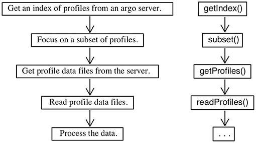
Figure 3. Typical work flow of the argoFloats package with description of the steps on the left, and names of the relevant functions on the right.

Once an index has been downloaded, the next step is usually to subset it according to some criterion. This is accomplished by using a function called subset() that specializes a generic R function. (The scheme of specializing generic functions is one of the reasons for the popularity of R, since it makes it easy to guess how to work with new types of data in familiar ways.) The subset() operation can be done in many different ways. These include isolating data by float ID, by cycle number, by time, by location, by institution, or by Deep category, etc. It is common to subset sequentially, often performing statistical analyses or producing graphs of the data at each step. To help an analyst keep track of the winnowing that occurs with each subset() call, the function prints a note on the fraction of data that were retained. It should be noted that finding subsets is a fast operation, because it does not involve file downloads.

Once a subset of interest has been specified, the next step is to download the netCDF files containing the data of interest, using getProfiles(). This function takes as primary input the return value of either getIndex() or subset(). Since the file sizes are of order 100 KB, this step can be slow if many files are needed. For this reason, getProfiles() follows the pattern set by getIndex(), caching downloaded files, so that future calls can use local files if they meet an age criterion. Therefore, getProfiles() tends to be a fast operation, except at the start of a new project.

The next step, accomplished with readProfiles(), is to read the local data. In most cases, this function uses the output of getProfiles(), but it is also possible to specify netCDF file names, skipping the previous steps.

Once data have been read, the user has an object in the R session that can be analyzed in a wide variety of ways. Generic functions are provided for some common tasks, with the prime components being as follows.

1. The summary() generic function provides an overview of the object.

2. The [[ generic function retrieves data from within an argoFloats object. For example, if A is an object returned by readProfiles(), then A[[''temperature'']] returns an R list object with one element for each profile stored in A. At this stage, the user can use standard R methods to perform a profile-by-profile analysis, to string the data together to get an overall view, etc.

3. The plot() generic function creates a variety of graphical displays of the data, e.g., maps of the positions of the Argo float(s), temperature-salinity diagrams, time-series plots of QC flags and data, and profile plots. Simple calls to plot() created most of the figures that follow in this paper, although some of them are further modified by adding features (extracted with [[) using standard R graphical functions for drawing symbols, lines, polygons, text, images, etc.

Further to the last point, it is worth noting that the use of [[ to extract data from argoFloats objects gives the user the freedom to use any of the statistical and other functions provided by R and its many thousands of contributed packages. Thus, although it might seem to be simple, the [[ function is actually a central contributor to the power and scope of argoFloats.

3. argoFloats Workflow Examples

3.1. Analysis of Float Trajectories

Figure 4 shows the path of the float 6900388 (that is, the float with World Meteorological Organization number 6900388) in the North Atlantic. Its construction followed the pattern outlined in Figure 3, although there was no need for the getProfiles() or readProfiles() stage because Argo index files contain float sampling times and locations, and together these things are all that is required to construct Figure 4. A simpler version of the plot, skipping the indication of time, is obtained with

FIGURE 4

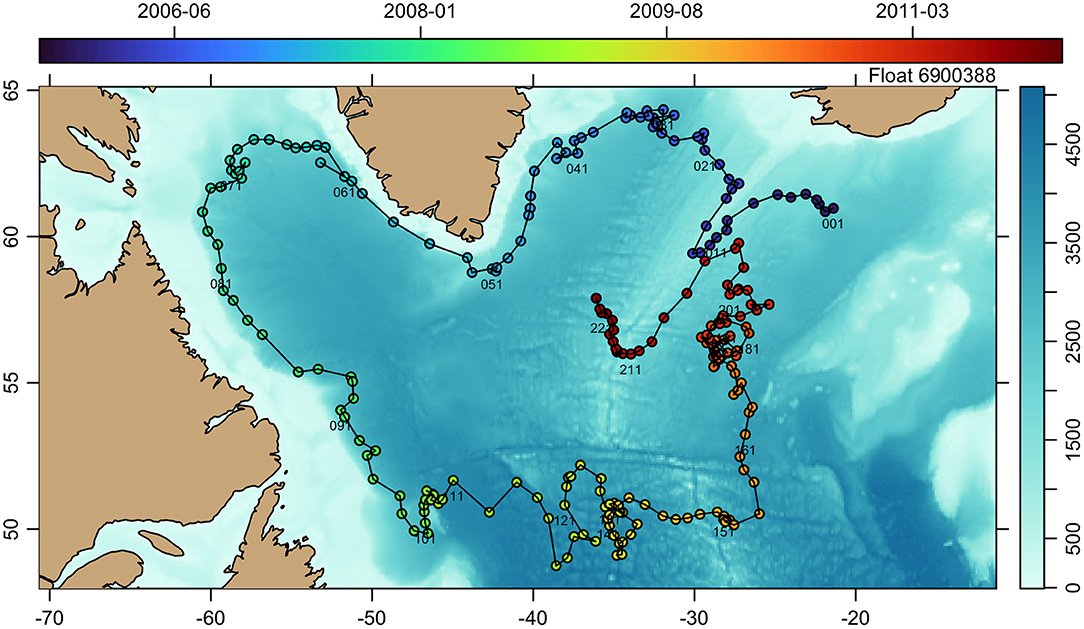
Figure 4. Trajectory of Argo float 6900388 circulating in the northwest Atlantic Ocean. Water depth is indicated in the color underlay, and sampling time is indicated with colored dots. Cycle numbers are labeled at regular intervals, indicating that this float made well over 200 cycles during its 5-year lifetime.

library(argoFloats)

index1  <- getIndex()

index2  <- subset(index1, ID="6900388")

plot(index2, bathymetry=TRUE)

and readers who run this code will find that the subset() call reveals that there are 223 cycles for this float. Two files will be downloaded in the process, one for the Argo index, and another (from a NOAA server) for a bathymetry file tailored to this geographical view. In many applications, the user will already have a local bathymetry file, so the second argument to plot() can be altered to use that, speeding up the process.

The main difference between the results of the preceding four-line operation and Figure 4 is the use of colored symbols to indicate float sampling times and the labeling of cycle numbers at some locations. The relevant information may be obtained with

time  <- index2[["time"]]

and similar steps, after which standard R functions (including colormap() and drawPalette() from the oce package) may be used to add other elements of Figure 4. This illustrates how argoFloats provide basic functionality for common tasks, while also making it easy for users to extend that functionality to meet their own needs.

It would be simple to extend this with the geodXy() function in oce, to learn more about ocean velocities at the float parking depth. Some smoothing or regression analysis might be required to achieve the desired results, and readers who are new to R may be pleased to learn how easy it is to carry out such analyses with standard R functions.

This first example has dealt only with index data, i.e., it has skipped the third and fourth steps in Figure 3. Many analyses will be similar to this (see e.g., the later section about a GUI application), but it is also important to illustrate how to download Argo netCDF data files with getProfiles() and how to read those data files with readProfiles(), as will be done in the next section.

3.2. Watermass Analysis

Temperature-salinity diagrams are a useful tool for watermass analysis, and a common first step is to prepare such diagrams showing water samples obtained in different areas. Figure 5 is a case in point. The first step in its construction was to use subset() to isolate a circle within a 150 km radius of Panama. The region was then subdivided into polygons separating the Atlantic and Pacific waters. The polygons were determined using plot(…,which=''map'') to get a map of the region, then using locator() to determine vertices on these selected polygons. (Note that subset() can choose data by ocean basin, but this is not accurate in this region, evidently owing to the limited resolution of the polygons used by the Argo processing system to designate ocean basins.) The fact that none of these steps takes more than a minute is an illustration of why people are drawn to R for interactive work. It is also worth noting that R makes it easy to follow such exploratory steps with algorithmic schemes, e.g., defining subsets that trace bathymetric contours or the boundaries of marine protected areas, or that establish Argo-based virtual moorings or ocean transit sections.

FIGURE 5

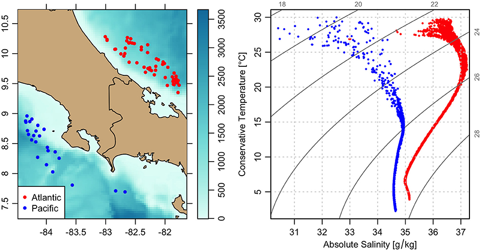
Figure 5. Contrast of water properties across the Isthmus of Panama. (Left) Locations of Argo cycles, color-coded by ocean. (Right) Temperature-salinity diagram showing the contrast between Atlantic and Pacific watermasses.

The right-hand panel of Figure 5 was made with plot(argos,which=''TS'',col=colBasin), where argos holds data obtained by applying readProfiles() to the output of getProfiles() for the relevant geographical regions and colBasin was defined to colorize by region. The resultant temperature-salinity diagram should make sense to readers with oceanographic experience, who are aware of a large contrast between Atlantic and Pacific watermass types. However, readers who try the procedure summarized above will find that there are many outliers that make no physical sense. This is because argoFloats works with the data as specified in the official data files, and these data are subject to error. As with many oceanographic datasets, Argo data are typically accompanied by QC flags. Using applyQC() on an argo object containing profiles turns questionable data into NA (missing) values, so they do not appear on the plot. This step was taken in the creation of Figure 5. The argoFloats package has several tools for the handling of QC flags, and it is important that users become familiar with them, because the official QC flags are not always entirely accurate.

3.3. Quality Control Analysis

Core, BGC, and Deep Argo data all undergo testing to ensure the data found at the Data Assembly Centers (“DACs”) are reasonably accurate. This is done on both “real-time” and “delayed” data. As is explained in the Argo User's Manual (Carval et al., 2019), real-time measurements are assigned a QC flag within a 24–48 h time frame, and delayed-mode are reexamined within 1–2 years by scientists who apply additional procedures to check the quality. In addition to the designation of QC flags, some data sets may be changed in recognition of the QC analysis or in light of improvements to instrument calibrations, etc., with the results being referred to as “adjusted” data.

It is important to note that even with vigorous testing procedures, QC flags cannot be considered perfect. As described in section 1.3 of the Argo User's Manual (Carval et al., 2019), the user assumes all risk using Argo data and, as will be demonstrated presently, careful analysts should consider applying their own QC checks to their data.

A three-step process can help with such work. First, use plot(…,which=''QC'') to plot an overview of the QC flags for the parameters of interest. In addition to showing QC flags, this function can also show the dataStateIndicator designation, which reveals the level of QC processing performed on individual float cycles. Second, use applyQC() to replace suspicious data with NA values, so they will not appear in plots or be considered in calculations, and create some diagnostic plots (e.g., temperature-salinity diagrams, profiles of temperature, salinity, and density) to assess whether applyQC() failed to remove some questionable data. Third, if there are such questionable data, use showQCTests() to get a summary of the QC tests (if any) that were performed on the data. (Perhaps surprisingly, different QC procedures are sometimes applied to different cycles for a given float.) The first and third of these steps might be skipped for quick work, but they should be carried out for in-depth analysis.

For example, Figure 6 shows a QC plot for float 1901584. Cursory examination indicates that, although the float reported data for nearly 5 years, the quality of those data declined seriously in its final 2 years. Another variant of the plot (not shown) reveals that the “data state indicator” was 2B for each profile made with this float, which according to Reference Table 6 of the Argo User's Manual (Carval et al., 2019) indicates that automated testing has been done, without additional scrutiny by scientists.

FIGURE 6

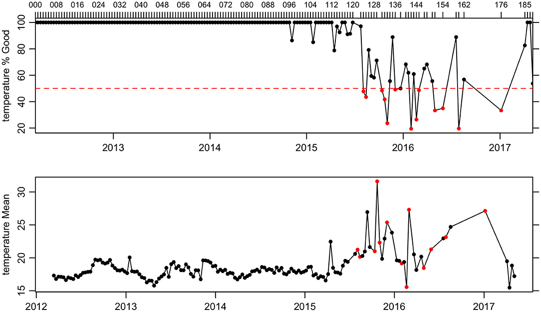
Figure 6. Quality Control plot for Argo float 1901584 near the Bahamas. The top panel shows the percent of data that are likely to be trustworthy, being described with QC flag codes 1 (meaning good data), 2 (probably good), 5 (changed), or 8 (estimated). Cycles are indicated with ticks at the top margin of this panel. The bottom panel shows the depth-averaged value of the parameter in question (temperature, in this example) regardless of the flag value, with red dots indicating cycles in which more than half the data are flagged as bad.

To this end, Figure 7 shows the impact of removing the “bad” data from this float using applyQC(). It will be obvious to anyone with oceanographic experience that the uncorrected data (left-hand panel) are heavily polluted with erroneous values. Indeed, the water properties are so far from typical oceanic values that the oce function that produces this plot does not even attempt to draw isopcynal curves across the whole panel. The coloring in this figure indicates that the wildest outliers have been flagged as questionable. The right-hand panel, which is cleared of flagged data, is more reasonable. However, and importantly, it also contains some points that are far from the main data cloud, and that would likely catch the attention of a experienced analyst.

FIGURE 7

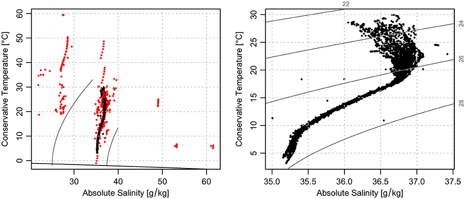
Figure 7. Effect of handling Argo QC flags for float 1901584 using applyQC(). (Left) temperature-salinity diagram showing all data, colored red if the QC flags indicate “bad” values with QC flag codes 3 (Probably bad data that are potentially correctable), 4 (Bad data), 6 (Not used), or 7 (Not used). (Right) similar diagram, but narrowed to data flagged as good. In the latter, note the existence of several points that depart widely from the data cloud, even though the QC flags have been accounted for.

One way to investigate such outliers on a temperature-salinity diagram is to consider the dependence of the seawater property called “spiciness,” which is in some sense orthogonal to density on such a diagram (Flament, 2002; McDougall and Krzysik, 2015). Figure 8 shows the results of such an analysis, in which a smoothing cubic spline was used to summarize the dependence of spiciness on potential density anomaly. The standard deviation δ of the difference between data and spline was computed, and then points that departed from the spline by more than 5δ were colored. This seems to identify outliers well, as can be seen when the data are redrawn in temperature-salinity space. A reasonable next step might be to compute density-dependent deviation, to account for the (expected) thickening of the data cloud for waters near the surface. There again, the standard R functions will greatly reduce the analysis effort.

FIGURE 8

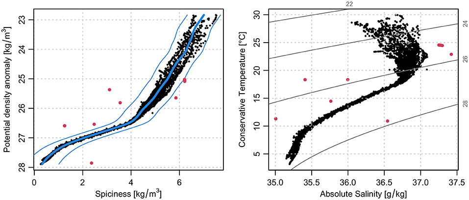
Figure 8. Demonstration of non-standard QC analysis based on scatter from the data cloud, using the same dataset as in Figure 7. (Left) covariation of potential density anomaly, σ_θ, and spiciness parameter, Π. The thick blue line is a smoothing spline expressing Π as a function of σ_θ, and the thinner lines indicate plausibility boundaries defined by 5 times the standard deviation of the model misfit. Points outside this boundary are colored red. (Right) temperature-salinity diagram as in Figure 7, but with red for points that are outside the Π(σ_θ) spline boundary.

Having identified a set of outlying points, either with an algorithm as in Figure 8 or by any other means, it is easy to determine which profiles contain those points, and then to use showQCTests() to learn which QC tests had been performed in each case. This can provide useful clues as to why suspicious data made their way onto the Argo data servers without being flagged. Another good practice is to produce profile plots for each case, highlighting the questionable points as a way to diagnose possible problems with existing QC procedures, and to help frame ideas for new tests, such as our new spiciness test.

3.4. Using Adjusted Data

Some data sets undergo adjustments that are made in recognition of the QC analysis or improved calibration, with the adjusted values being stored within data files alongside the raw (original) values. Adjustments tend to be more common with BGC data than with Core data, perhaps owing to issues relating to sensor maturity (Thierry et al., 2018).

The argoFloats function named useAdjusted() provides a convenient way of dealing with such data. It works by optionally copying adjusted data into the locations that normally store raw data. This causes subsequent calls to plot and [[ to focus on the adjusted data, as opposed to the raw data. By default, useAdjusted() carries out replacement for all fields that have adjusted values. However, the function has an optional argument that causes it to replace only adjusted- and delayed-mode data, skipping over real-time data. This option can useful, because real-time adjusted data are always equal to missing values, leaving spatial/temporal gaps that raw data can help to fill in.

An example of using adjusted values is provided in Figure 9, which displays raw and adjusted oxygen profiles for cycle 001 of float 5903586, which sampled for about 2.5 years along the coast of Saudi Arabia. The diagram was made in two steps. First, raw data were read in and plotted with the argoFloats version of plot(), supplied with arguments indicating to show a profile of oxygen. Second, a new object was created with adjusted <- useAdjusted(raw), so that [[ would return adjusted values. Then, the adjusted pressure and oxygen concentration were accessed with [[, and plotted on the diagram, along with a legend, using standard R function calls. As in the preceding temperature-salinity example, it is worth noting that argoFloats is designed to provide only basic plots, with the user relying on standard R functions to add extra features. This eases the burden on users who are familiar with R, and helps to teach others how to use R for general tasks.

FIGURE 9

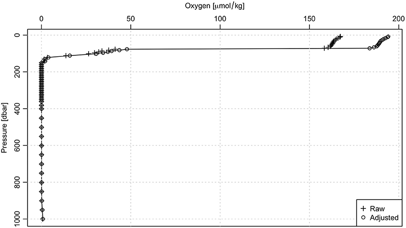
Figure 9. Demonstration of the useAdjusted() function for oxygen measurements (in μmol/kg) made during cycle 001 of Argo float 5903586.

4. Interactive Float Mapping Tool

The mapApp() function launches a GUI-based application for examining float locations, using the powerful R-shiny system (Chang, 2020). Initially, this shows a world view, with dots representing the locations of Argo float profiles within a selected time interval. Different colors are used for Core, BGC, and Deep profiles.

Multiple GUI elements make it easy to explore the data. Buttons control which float styles to display, whether to display bathymetry, whether to use low- or high-resolution coastlines, whether to draw line segments joining successive float locations, whether to draw starting and ending points on float trajectories, and so forth. There are also buttons to move the focus view around the earth, and to control the size of the display area. Text-entry fields are used to select a time interval to display, and there is a field in which the user can enter the ID of a particular float of interest. In addition, the system monitors the mouse location, with a click-slide action causing zooming to the indicated region, a hovering action causing a display of information about the nearest float profile, and a double-clicking action causing a float ID to be entered into the ID selection box. There is a simple way to switch from a multi-float view in a given time range to a view of the historical trajectory of a selected float, which can be quite helpful in finding datasets of interest for further exploration.

Other controls permit other actions, all of which are both documented and reasonably self-evident. Of particular note is a button that displays the argoFloats code that would produce the indicated view, starting from a getIndex() call, followed by subset() calls to isolate the data in question, and followed by hints on further actions that the user might undertake, including plots similar to those shown in previous sections of this document.

For example, Figure 10 shows a view of BGC float 6901181. Entering that float number in the float-ID box will reveal that this float was deployed in November 2015, near the western end of the trajectory, at the 43.6W and 51.0N. The black square by one of the points toward the European continent indicates the latest position of the float, at 20.9W and 43.3N. The complexity of the ocean circulation is revealed clearly in the complex shape of the trajectory between these two locations. Readers interested in exploring this float in more detail might find it helpful to start by using mapApp() to reproduce Figure 10, after which clicking on the Code button will reveal the argoFloats function calls needed to isolate the data, and, for example, plot a temperature-salinity diagram.

FIGURE 10

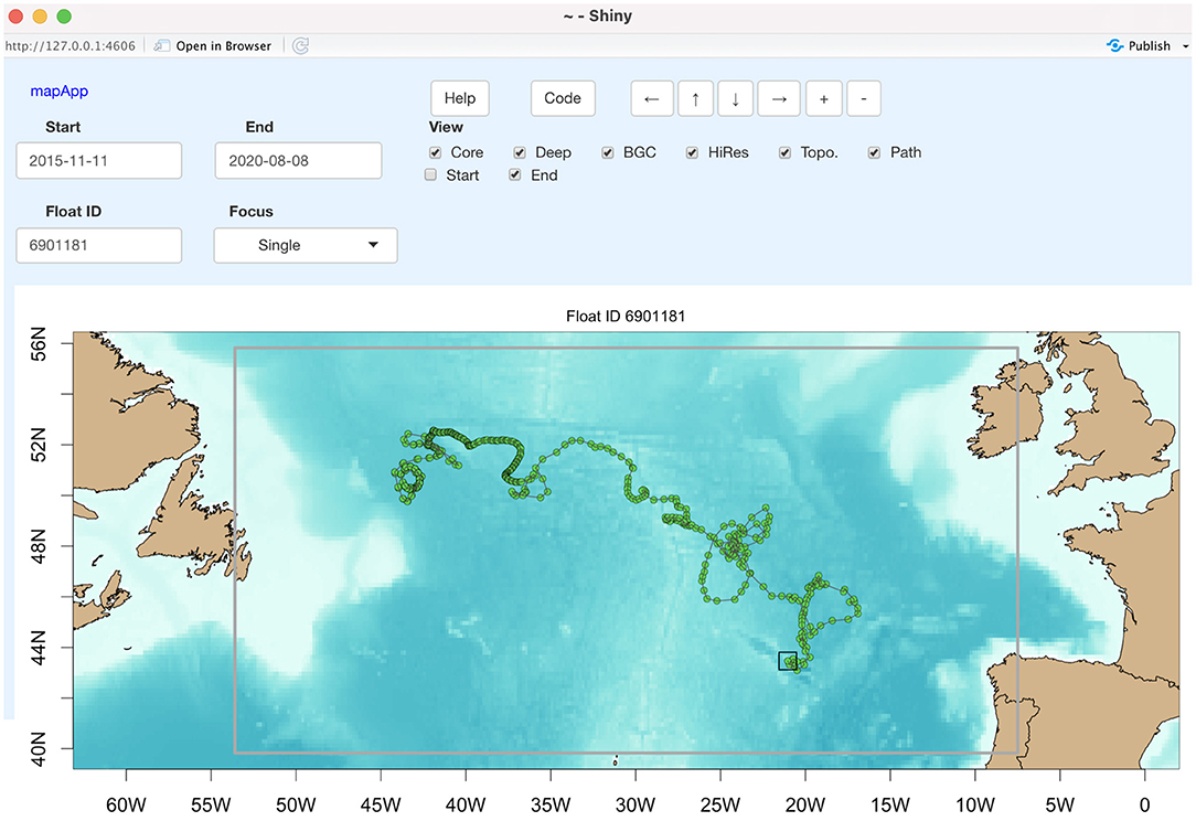
Figure 10. The mapApp() application, showing the trajectory of BGC float 6901181 in the North Atlantic. The elements in the top part of the interface are user controls, e.g., this view shows the float path, with the final position highlighted with a box.

5. The Future of argoFloats

As sketched above, argoFloats already provides a variety of tools for advancing Argo data analysis. However, it is still in a phase of active development, during which the developers are responding to community needs. The core functions, getIndex(), subset(), and [[, have proven to be suitable for everyday work, and are unlikely to change greatly. The same cannot be said of plot(), which is likely to continue to gain significant new features soon, to accommodate the fairly wide variety of oceanographic plot styles. Similarly, there are plans to complement the mapApp() tool with other tools that provide more in-depth analysis of Argo data.

From the start, argoFloats has taken a practical approach to most problems. Newcomers to Argo data tend to find it difficult to download data using FTP tools or the server websites, so getIndex() was created to help in this task. Isolation of particular floats for a given purpose is also challenging, and so subset() was created. Reading the files that store Argo profile data demands skills not just in reading netCDF but also in linking the actual data elements with their associated metadata, such as QC flags and units. Users are relieved of such burdens by readProfiles(), which in itself relies on lower-level functions provided by the oce package. Similarly, oce is relied upon for the various oceanography-specific operations such as the handling of QC flags, computation of Absolute Salinity and Conservative Temperature from measured properties, the construction of temperature-salinity diagrams, etc.

At this time, argoFloats handles many practical tasks that are required by a research team of university and government scientists. While this is a good start, we feel certain that the package will benefit from a wider base of users and developers. For this reason, we are employing an open-source model for both coding and collaboration, and we hope this paper will get others interested in this community project.

Data Availability Statement

The datasets analyzed for this study were downloaded in November 2020 from the Argo servers ftp.ifremer.fr and ftp://usgodae.org/pub/outgoing/argo.

Author Contributions

CR conceived of the idea and secured the initial support for the work and participated in discussions and planning. DK and JH wrote the majority of the code in the package. DK and CR shared in salary support for JH. DK and JH wrote the text. CR helped to edit it. All authors contributed to the article and approved the submitted version.

Funding

Funding support for JH was through Fisheries and Oceans Canada's commitment under the G7 Charlevoix Blueprint for Healthy Oceans, Seas and Resilient Coastal Communities, and through an NSERC Discovery Grant (number 03740) to DK.

Conflict of Interest

The authors declare that the research was conducted in the absence of any commercial or financial relationships that could be construed as a potential conflict of interest.

Acknowledgments

We are indebted to the two reviewers of this manuscript, for their detailed and insightful comments. We also thank Dewey Dunnington, Chris Gordon, and Blair Greenan of the Department of Fisheries and Oceans Canada, for their advice on the early manuscript. Dewey Dunnington contributed to the argoFloats package, while Chris Gordon advised us on Argo quality control. Chris Gordon and Dewey Dunnington provided comments on the manuscript. Blair Greenan is the Scientific Director of Argo Canada, and contributed support for the work, including the hiring of JH.

Footnotes

1. ^https://fleetmonitoring.euro-argo.eu/dashboard.

2. ^ftp.ifremer.fr.

3. ^usgodae.org.

References

Argo (2020). Argo float data and metadata from Global Data Assembly Centre (Argo GDAC). SEANOE. Available online at: https://www.seanoe.org/data/00311/42182.

Bittig, H. C., Maurer, T. L., Plant, J. N., Schmechtig, C., Wong, A. P. S., Claustre, H., et al. (2019). A BGC-Argo guide: planning, deployment, data handling and usage. Front. Mar. Sci. 6:502. doi: 10.3389/fmars.2019.00502

CrossRef Full Text | Google Scholar

Boyer, T. P., Baranova, O. K., Coleman, C., Garcia, H. E., Grodsky, A., Locarnini, R. A., et al. (2018). World Ocean Database (2018). Silver Springs, MD: National Centers for Environmental Information Ocean Climate Laboratory.

Google Scholar

Carval, T., Keeley, B., Takatsuki, Y., Yoshida, T., Loch, S. L., Schmid, C., et al. (2019). Argo User's Manual V3.3 (Ifremer).

Google Scholar

Chang, W. (2020). Shiny: Web Application Framework for R. Available online at: https://CRAN.R-project.org/package=shiny (accessed November 24, 2020).

Flament, P. (2002). A state variable for characterizing water masses and their diffusive stability: spiciness. Prog. Oceanogr. 54, 493–501. doi: 10.1016/S0079-6611(02)00065-4

CrossRef Full Text | Google Scholar

Gasparin, F., Hamon, M., Rémy, E., and Le Traon, P.-Y. (2020). How deep Argo will improve the deep ocean in an ocean reanalysis. J. Clim. 33, 77–94. doi: 10.1175/JCLI-D-19-0208.1

CrossRef Full Text | Google Scholar

Kelley, D., Harbin, J., and Richards, C. (2020a). argoFloats. Available online at: https://github.com/ArgoCanada/argoFloats (accessed November 24, 2020).

Kelley, D., Harbin, J., and Richards, C. (2020b). argoFloats: Analysis of Oceanographic Argo Floats. Available online at: https://argocanada.github.io/argoFloats/index.html (accessed November 24, 2020).

Kelley, D., and Richards, C. (2020). oce: Analysis of Oceanographic Data. Available online at: https://CRAN.R-project.org/package=oce (accessed November 24, 2020).

Kelley, D. E. (2018). Oceanographic Analysis With R. New York, NY: Springer-Verlag.

Google Scholar

Maze, G., and Balem, K. (2020). Argopy: a Python library for Argo ocean data analysis. J. Open Sour. Softw. 5:2425. doi: 10.21105/joss.02425

CrossRef Full Text | Google Scholar

McDougall, T. J., and Krzysik, O. A. (2015). Spiciness. J. Mar. Res. 73, 141–152. doi: 10.1357/002224015816665589

CrossRef Full Text | Google Scholar

Nguyen, A. T., Heimbach, P., Garg, V. V., Ocaña, V., Lee, C., and Rainville, L. (2020). Impact of synthetic arctic Argo-type floats in a coupled ocean-sea ice state estimation framework. J. Atmos. Ocean. Technol. 37, 1477–1495. doi: 10.1175/JTECH-D-19-0159.1

CrossRef Full Text | Google Scholar

Ollitrault, M., and Rannou, J.P. (2013). ANDRO: An Argo-Based Deep Displacement Dataset. J. Atmos. Ocean. Technol. 30, 759–788. doi: 10.1175/JTECH-D-12-00073.1

CrossRef Full Text | Google Scholar

R Core Team (2020). R: A Language and Environment for Statistical Computing. Vienna: R Foundation for Statistical Computing. Available online at: https://www.R-project.org/ (accessed November 24, 2020).

Google Scholar

Roemmich, D., Alford, M. H., Claustre, H., Johnson, K., King, B., Moum, J., et al. (2019). On the future of Argo: a global, full-depth, multi-disciplinary array. Front. Mar. Sci. 6:439. doi: 10.3389/fmars.2019.00439

CrossRef Full Text | Google Scholar

Roemmich, D., Johnson, G. C., Riser, S., Davis, R., Gilson, J., Owens, W. B., et al. (2009). The Argo program: observing the global ocean with profiling floats. Oceanography 22, 34–43. doi: 10.5670/oceanog.2009.36

PubMed Abstract | CrossRef Full Text | Google Scholar

Schmid, C., Molinari, R. L., Sabina, R., Daneshzadeh, Y.-H., Xia, X., Forteza, E., et al. (2007). The real-time data management system for Argo profiling float observations. J. Atmos. Ocean. Technol. 24, 1608–1628. doi: 10.1175/JTECH2070.1

CrossRef Full Text | Google Scholar

Thierry, V., Bittig, H., and The Argo-BGC Team (2018). Argo Quality Control Manual for Dissolved Oxygen Concentration.

Google Scholar

Tucker, T., Giglio, D., Scanderbeg, M., and Shen, S. S. P. (2020). Argovis: a web application for fast delivery, visualization, and analysis of Argo data. J. Atmos. Ocean. Technol. 37, 401–416. doi: 10.1175/JTECH-D-19-0041.1

CrossRef Full Text | Google Scholar