
94% of researchers rate our articles as excellent or good
Learn more about the work of our research integrity team to safeguard the quality of each article we publish.
Find out more
ORIGINAL RESEARCH article
Front. Mar. Sci. , 25 June 2021
Sec. Coastal Ocean Processes
Volume 8 - 2021 | https://doi.org/10.3389/fmars.2021.633707
 Zhengui Wang1
 Fei Chai1*
 Huijie Xue1
 Xiao Hua Wang2Yinglong J. Zhang3Richard Dugdale4
 Frances Wilkerson4
In San Francisco Bay (SFB), light availability is largely determined by the concentration of suspended particulate matter (SPM) in the water column. SPM exhibits substantial variation with time, depth, and location. To study how SPM influences light and phytoplankton growth, we coupled a sediment transport model with a hydrodynamic model and a biogeochemical model. The coupled models were used to simulate conditions for the year of 2011 with a focus on northern SFB. For comparison, two simulations were conducted with ecosystem processes driven by SPM concentrations supplied by the sediment transport model and by applying a constant SPM concentration of 20 mg l–1. The sediment transport model successfully reproduced the general pattern of SPM variation in northern SFB, which improved the chlorophyll-a simulation resulting from the biogeochemical model, with vertically integrated primary productivity varying greatly, from 40 g[C] m–2 year–1 over shoals to 160 g[C] m–2 year–1 in the deep channel. Primary productivity in northern SFB is influenced by euphotic zone depth (Ze). Our results show that Ze in shallow water regions (<2 m) is mainly determined by water depth, while Ze in deep water regions is controlled by SPM concentration. As a result, Ze has low (high) values in shallow (deep) water regions. Large (small) differences in primary productivity exist between the two simulations in deep (shallow) water regions. Furthermore, we defined a new parameter Flight for “averaged light limitation” in the euphotic zone. The averaged chlorophyll-a concentration in the euphotic zone and Flight share a similar distribution such that both have high (low) values in shallow (deep) water regions. Our study demonstrates that light is a critical factor in regulating the phytoplankton growth in northern SFB, and a sediment transport model improves simulation of light availability in the water column.
San Francisco Bay (SFB) is the largest estuary along the US west coast. A healthy ecosystem in SFB is important not only to San Francisco Bay the millions of people populated around it but also to the resident birds and fishes (Warnock and Takekawa, 1995; Novick and Senn, 2014). However, the bay has been considered a high-nutrient, low-chlorophyll (HNLC) system since the 1980s (Cloern, 2001; Dugdale et al., 2012), especially in the northern part of the bay, which has led to a decline in ecologically important species like the delta smelt (Sommer et al., 2007; Dugdale et al., 2013). Geographically, SFB includes a well-mixed lagoon in the south, a central embayment connected to the ocean, and a partially mixed estuary of two sub-embayments (San Pablo Bay and Suisun Bay) in the north (Cloern, 1987; Liu et al., 2018). Two large rivers, the Sacramento River and San Joaquin River, flow into the system from the north with the majority of freshwater input in winter and spring (Buchanan and Ganju, 2007; U.S. Geological Survey, 2014). The tides in SFB are dominated by semi-diurnal constituents with a mean tidal range of 1.28 m and a prominent spring–neap tidal cycle (Cloern and Nichols, 1985; Elias and Hansen, 2013). The wind in SFB has a noticeably seasonal cycle with strongest winds in summer (Conomos et al., 1985). Among the different nutrient sources into SFB, waste water treatment plants (WWTPs) and discharge from rivers are the most important. Nutrient load from the WWTPs to the northern SFB is mainly in the form of NH4 (about 34,300 kg day–1), while nutrient loads associated with river discharge is mainly in the form of NO3 (about 10,400 kg day–1) (Novick and Senn, 2014). Despite the large nutrient input, the primary production in SFB is low (Cloern and Jassby, 2012; Dugdale et al., 2016) and nutrients are exported into the ocean (Wang et al., 2020), except during some episodic phytoplankton bloom events in response to climate anomalies (Cloern et al., 2005, 2010).
To explain the HNLC phenomenon in SFB, there have been numerous studies of the different factors that impact phytoplankton growth. Cloern (1987) concluded turbidity to be a major control on estuarine phytoplankton by driving light availability. A high concentration of suspended particulate matter (SPM) caused by river inflow, tides, and waves (Bever and MacWilliams, 2013) can result in poor light condition and subsequent low primary production in SFB. Dugdale et al. (2013) and Wilkerson et al. (2015) examined the combined influence of river inflow and nutrient concentration on phytoplankton growth in Suisun Bay and found that the lack of phytoplankton blooms may be due to high NH4 concentrations (above 4 mmol m–3) that inhibit phytoplankton from accessing the dominant DIN nutrient pool of NO3. Lucas et al. (2009) investigated the relationship between phytoplankton growth rate and transport time using a conceptual model and suggested that low chlorophyll concentration may also be due to short transport time related to high river inflow (Wang et al., 2019). Additionally, Dugdale et al. (2016) and Lucas et al. (2016) studied the benthic grazing of Asian invasive clams that entered SFB in the late 1970s and concluded clam grazing to be another factor responsible for the low chlorophyll concentration in SFB. These studies each address one aspect linked to the potential low primary production in SFB. By using a 3D biogeochemical model, Liu et al. (2018) integrated all these factors together in an SFB ecosystem simulation and investigated their interaction along with the sensitivity of phytoplankton biomass to these factors. Wang et al. (2020) used a similar model configuration but conducted a 10-years model simulation, to evaluate nutrient export from SFB to the ocean. These numerical models provide a useful tool to disentangle different aspects of the ecosystem and identify the important factors that regulate the phytoplankton growth in SFB.
Turbidity is an important environmental factor that regulates the light availability for primary production. It is largely affected by SPM concentration in SFB (Cloern, 1987). As a result, the phytoplankton growth is largely regulated by SPM concentration that impacts the water transparency. The SPM concentration in SFB has substantial temporal and spatial variability and can range from several milligrams to hundreds of milligrams per liter (Buchanan and Ganju, 2007; Schoellhamer et al., 2008). During the wet period in winter and spring, large quantities of suspended sediment are transported into the estuary along with river inflow from the bay delta region (Schoellhamer et al., 2008). During the following dry period, the sediment is redistributed inside the bay through advection, deposition, and resuspension; eventually, some of the sediment is exported to the coastal ocean (Barnard et al., 2013). SPM concentration is modulated by tides and wind waves on short timescales (Buchanan and Ganju, 2007; Bever and MacWilliams, 2013). Schoellhamer et al. (2008) studied the SPM measurements at different depths and showed that wind-driven currents and waves can resuspend sediment in shallow water, while tides resuspend sediment in deep water. On large scales, wind is an important factor in controlling the estuarine circulation, which impacts the sediment transport in SFB. There also exists considerable vertical SPM variation, with higher concentrations in the bottom water compared to surface water (U.S. Geological Survey Data, 2018). In SFB, SPM concentration varies greatly with location. The sediment dynamics in SFB are further complicated by different sediment sources, variable flow transport, different sediment particle sizes, and sediment bed properties (Barnard et al., 2013). Sediment transport models that account for all these factors are useful in simulating the complex variation of SPM in SFB. Schoellhamer et al. (2012) developed a conceptual sediment transport model to qualitatively describe sediment distribution in the bay delta. Bever and MacWilliams (2013) developed a dynamic sediment transport model for San Pablo Bay, which was coupled with a hydrodynamic model and a wave model, to simulate spatiotemporal variability of sediment flux in the region.
Even so, no models incorporating SPM have focused on how the variation in SPM affects light condition and phytoplankton growth in SFB. In this study, we address this by coupling a sediment transport model with a hydrodynamic model and a biogeochemical model. The simulated SPM concentration resulting from the sediment transport model is used to compute light availability for phytoplankton growth in the biogeochemical model. The sediment transport model ‘‘SED3D’’ is a part of the ‘‘Semi-implicit Cross-scale Hydroscience Integrated System Model’’ (SCHISM) modeling system1; it can simulate advection, diffusion, and settling of multiple non-cohesive sediment classes in the water column as well as sediment deposition and erosion at the bottom (Pinto et al., 2012). The hydrodynamic model used is the SCHISM, which is a derivative of the original “Semi-implicit Eulerian–Lagrangian Finite-Element model” (SELFE) (Zhang and Baptista, 2008), but with many enhancements including a new extension to cover large-scale eddying regimes and a seamless cross-scale modeling capability from creek to ocean (Zhang et al., 2016). The biogeochemical model used is the “CoSiNE” model, which stands for “Carbon, Silicate, Nitrogen Ecosystem” (Chai et al., 2002, 2007). CoSiNE can be used to simulate biogeochemical processes involving nutrients, phytoplankton, zooplankton, and detritus. The combination of these three models integrates the SFB estuarine circulation, sediment transport process, and phytoplankton dynamics, enabling us to investigate the effect of SPM variation due to sediment on phytoplankton growth. In this study, we used the sediment transport model to obtain estimates of SPM and focused on the effect of SPM on regulating light condition. The paper is organized as follows: model configuration is described in the “Materials and Methods” section, followed by modeling results in the “Results” and “Discussion” sections. Finally, the “Summary” section is given.
The configuration of SCHISM is based on Chao et al. (2017). The model domain covers the entire SFB, extending from Coyote Creek in the South Bay to Rio Vista in the north. In addition, part of the coastal ocean outside of the SFB entrance (the Golden Gate) is included. The model grid includes coarse resolution in shallow water areas and fine resolution in the deep channel, varying from 10 to 100 m. Water depth along the channel can change from less than 10 m to more than 30 m (Chao et al., 2017), though it is generally less than 3 m in the broad shallow shoals (Cloern, 1987). In the vertical, we used 23 sigma layers. The hydrodynamic model is driven by atmospheric forcing including wind and solar radiation (Doyle et al., 2009), river inflows at river boundaries, and oceanic forcing (including water level and velocity at the coastal boundary). The time step is 120 s.
The configuration of CoSiNE is based on Liu et al. (2018) and Wang et al. (2020). The CoSiNE model has 13 state variables with two zooplankton species, two phytoplankton groups, four inorganic nutrients, two kinds of detritus, dissolved oxygen, carbon dioxide, and alkalinity. The setup for CoSiNE model includes concentrations for these variables at both river and ocean boundaries. The effluents from the WWTPs within the SFB (Novick and Senn, 2014) are added as nutrient sources for the ecosystem. More detailed specification of these inputs can be found in Liu et al. (2018), and the model parameter values are shown in Table A1. In this study, a modification was made to the phytoplankton concentration at river boundaries. The input in Liu et al. (2018) and Wang et al. (2020) was based on the monthly water quality measurements (grab sample) by the United States Geological Survey (USGS) (Schraga and Cloern, 2017), while here we use continuous monitoring data collected at 15-min intervals from the California Data Exchange Center at the Department of Water Resources2 (DWR).
Southern SFB is distinctly different from the northern bay, in terms of geomorphology and hydrodynamic circulation (Cloern, 1987; Cloern and Jassby, 2012). In this study, we focused on the ecosystem in northern SFB. The domain includes San Pablo Bay and Suisun Bay (Figure 1), which are under heavy influences from river discharge and sediment input from the bay delta (Dugdale et al., 2012; Barnard et al., 2013). The simulation was carried out for the year 2011, a wet year, during which a large river inflow occurred in March and April (U.S. Geological Survey Data, 2018). Figure 1 shows the model grid, along with two USGS stations of turbidity measurements3, two DWR stations of chlorophyll-a measurements, and six USGS stations of water quality measurements.
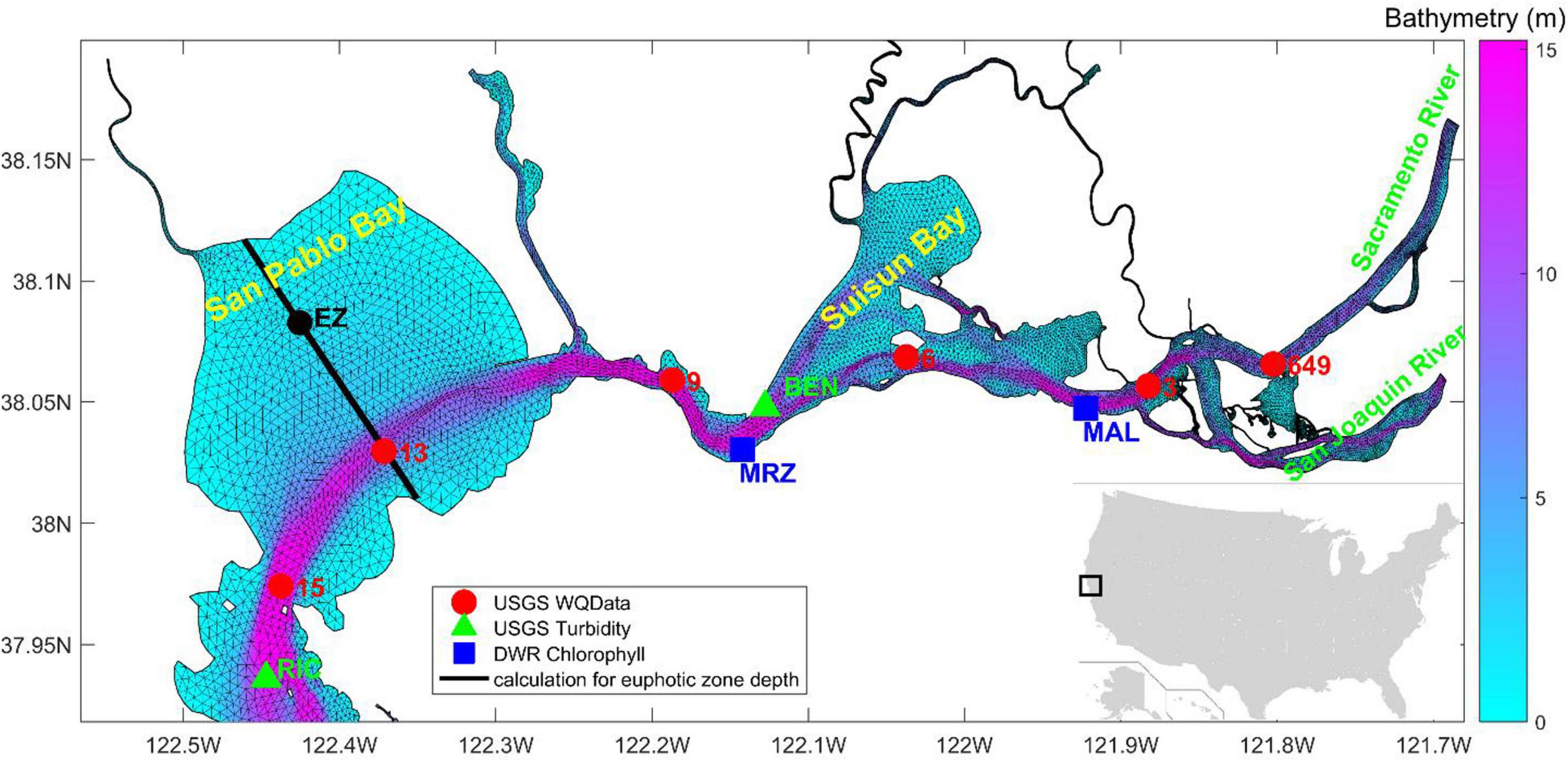
Figure 1. Model grid in northern San Francisco Bay (SFB) with bathymetry superposed. Markers represent the United States Geological Survey (USGS) monitoring stations (USGS 15, 13, 9, 6, 3, and 649) for monthly water quality data, turbidity data (RIC and BEN), as well as DWR chlorophyll-a data (MRZ and MAL). The black line in San Pablo Bay is a transect along which euphotic zone depth is analyzed.
The sediment transport model SED3D shares the same model grid as SCHISM and CoSiNE, but its configuration requires specification of sediment model variables in both sediment bed and water column. In this study, we considered only one sediment bed layer and three sediment grain size classes: 0.02, 0.10, and 0.60 mm in diameter. The critical shear stress and settling velocity of sediment grains are computed by SED3D. The initial sediment porosity was set to 0.4, and bed fraction for each grain class is one third. In the water column, the initial SPM concentration was set to 25 mg l–1. In addition, we assigned the SPM concentrations at river boundaries based on turbidity measurement data using a linear relationship between SPM concentration and turbidity measurement (Buchanan and Ganju, 2007). More information about SED3D can be found in Pinto et al. (2012) and http://ccrm.vims.edu/schismweb/.
To investigate the impact of SPM on the ecosystem, we carried out two simulations. The coupled model SCHISM + CoSiNE was first run with a constant SPM concentration of 20 mg l–1, referred to as “SPM_20.” This SPM concentration of 20 mg l–1 is close to the average SPM concentration in SFB in 2011 and was also used by Liu et al. (2018) in their ecosystem simulation about SFB. Then, the fully coupled model SCHISM + CoSiNE + SED3D was run using SPM concentration generated from SED3D, referred to as “SPM_SED3D.”
In order to validate the sediment transport model, the simulated SPM results were compared with two types of observations. For the high-frequency variability, we first estimated SPM concentrations based on turbidity data (Buchanan and Ganju, 2007) and then compared them with the high-frequency modeled SPM result. For the long-term mean SPM values, monthly SPM measurements by the USGS were available at multiple locations in SFB (Schraga and Cloern, 2017). Because only one SPM data point was available at each individual location each month, while the model outputs SPM result hourly, it is inappropriate to directly compare the model results with those discrete observations. Therefore, we conducted a model error analysis by using the closest modeled SPM concentrations that occurred ±3 days around the observation times (see Table 1). The same statistical method was also used for the comparison between simulated chlorophyll-a and monthly chlorophyll-a measurements.
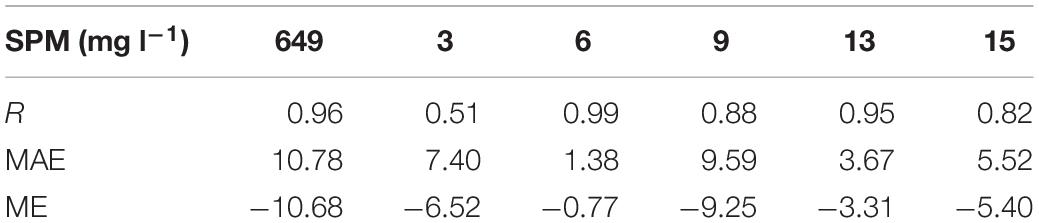
Table 1. Statistics for modeled surface suspended particulate matter (SPM) compared with monthly observational data at six USGS stations; statistics are based on the best matches in ±3 days around the observations, including correlation coefficient (R), mean absolute error (MAE), and mean error (ME).
In this study, we also investigated how tide regulates phytoplankton growth by impacting the light field in SFB. To quantitatively identify the signals of tidal frequencies, time series of chlorophyll-a and SPM at location MRZ were analyzed in frequency domain through Fourier transform for both model results and observations in “Influence of Tides” section.
Euphotic zone depth (Ze) is commonly used to represent the light penetration in water, which is often defined as the depth of 1% light level relative to surface light intensity I0 (Sellner et al., 2003; Muylaert et al., 2005). Because chlorophyll-a concentration is normally low in SFB and turbidity in the water column is often linearly correlated with SPM (Cloern, 1987; Buchanan and Ganju, 2007), we attribute the variation of Ze mainly to the variation of SPM concentration, with little contribution by chlorophyll-a attenuation. Therefore, simplistically in SFB, Ze represents how SPM impacts light penetration in the water.
In CoSiNE, the light factor for phytoplankton growth (Platt et al., 1980, 1982; Miller and Wheeler, 2012) is defined as follows:
Where μmax is maximum growth rate (day–1), α is initial slope of the P–I curve (w–1 m2 day–1), β is the slope for photoinhibition (w–1 m2 day–1), and I is light intensity (w m–2). Due to the high SPM concentration in controlling the light field in SFB, we ignore the photoinhibition effect by setting β = 0, and ϕ(z) is mainly used to simulate the light limitation effect in this study. Light intensity is determined by (Liu et al., 2018), where I0 is light intensity at water surface (w m–2) and k1(m–1), k2 (mmol–1 m2), and k3 (g–1 m2) are light attenuation coefficients for seawater, chlorophyll-a, and SPM, respectively. Colored dissolved organic matter (CDOM) is an important factor for the light attenuation (Babin et al., 2003). In SFB, the influence from SPM dominates over CDOM (Fichot et al., 2016). Thus, CDOM effect is omitted in CoSiNE model for this study.
The light factor (ϕ) represents the effect of both light and photosynthesis efficiency, and euphotic zone depth (Ze) represents how deep photosynthesis can happen in the water column. However, either the light factor or euphotic zone depth can represent the mean light condition for phytoplankton growth for the bulk water column in the euphotic zone. To describe the overall light availability, we defined a new parameter of “averaged light limitation” in euphotic zone that combines these two parameters as follows:
Where ϕ(z) is the light factor for phytoplankton (Eq. 1). Flight is a non-dimensional number. When Flight is close to one, it means phytoplankton growth is not limited by light availability in the euphotic zone. When Flight is close to zero, it means phytoplankton growth is completely limited by light.
For later model analysis, the primary productivity (PP) in CoSiNE model is computed as follows:
Where NPS1 (RPS1) is the NO3 (NH4) uptake (mmol m–3 day–1) by small phytoplankton, NPS2 (RPS2) is the NO3 (NH4) uptake (mmol m–3 day–1) by diatoms, and 7.3 is the conversion constant from nitrogen to carbon (Chai et al., 2007).
Figure 2 shows simulated near-surface SPM concentrations from the three-way coupled models, from April to May at two stations of BEN and RIC. Superimposed are USGS observations converted from turbidity measurements. The results from SED3D give correlation coefficients (R) of 0.56 and 0.85 and mean absolute errors (MAE) of 10.1 and 7.1 mg l–1, at the two stations, respectively, with respect to the observations. SED3D reproduces the tidal components of SPM variation as well as the SPM difference between the two stations. The model captures the general patterns of SPM observations at both stations, but with many discrepancies of underestimates and overestimates in details as SPM observational data have substantial variations associated with large uncertainties. For example, during the period from April 1st to April 15th, the modeled SPM at Station BEN only captures the mean, but overestimates the daily variations. Figure 2 shows that SPM concentration in SFB is highly variable over time. Both model results and observations display prominent diurnal variation. Some semi-diurnal signal can also be visually identified at RIC, particularly around April 20th where the model largely underestimates the signal. These diurnal and semi-diurnal variations are induced by tides, which resuspend sediment particles from the bottom as reported in Schoellhamer et al. (2008). There exists significant SPM variation with the spring–neap tidal cycle, which can significantly modify the amplitude of daily variation. For example, the maximum daily SPM concentration at RIC reached about 100 mg l–1 at spring tide time around May 18th, but fell below 20 mg l–1 at neap tide around May 25th. There are some subtle differences of SPM variation between the two stations. The lower values of SPM concentration at BEN are around 20 mg l–1, while the lower values at RIC can approach zero. Also, the tidal signals at RIC seem to be more regular with evident oscillations of diurnal and semi-monthly periods than those at BEN. These differences may be caused by the local hydrodynamics and partially related to the fact that RIC is closer to coastal ocean and therefore receives more oceanic influence, while BEN is located more upstream near Suisun Bay and receives more fluvial influence. Because the estimated SPM from turbidity data contains large uncertainties as the relationship between turbidity and SPM is highly variable (Buchanan and Ganju, 2007), the matches between modeled SPM and observation should not be over-interpreted, especially in the details.
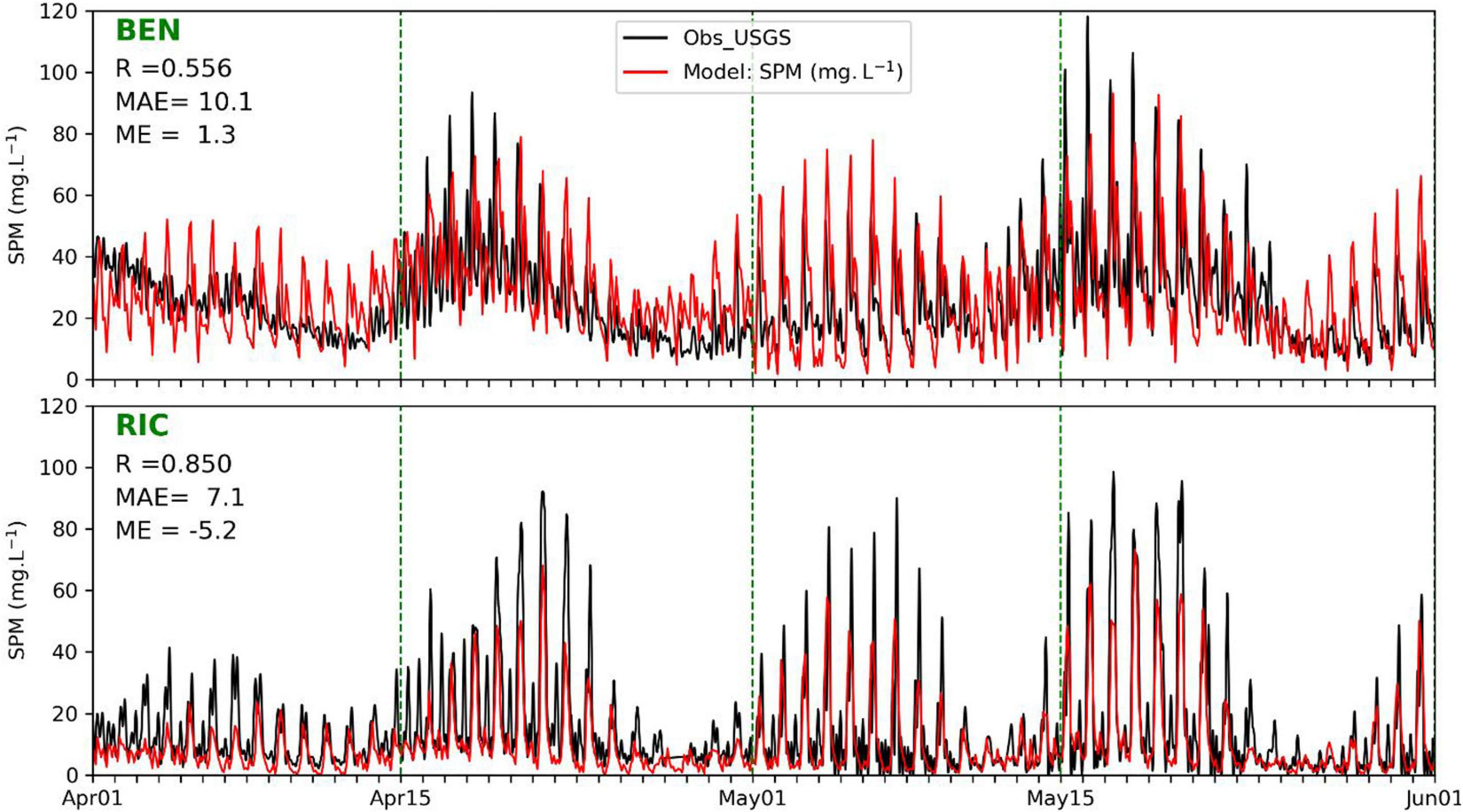
Figure 2. Comparison of near-surface suspended particulate matter (SPM) concentrations (mg l–1) between USGS observations and model results in SPM_SED3D. The observational data are converted from turbidity data following Buchanan and Ganju (2007). Statistics shown in the figure are correlation coefficient (R), mean absolute error (MAE), and mean error (ME).
Table 1 shows the comparison with monthly observational data at six bay channel stations (Figure A1). The R varies from 0.51 to 0.99. Note that the large R values in Table 1 merely represent observational data falling within the daily ranges of modeled SPM, given the statistical method adopted. The MAE of SPM varies from 1.38 to 10.78 mg l–1. The mean error (ME) are all negative, varying from −10.68 to −0.77 mg l–1, which suggests that the sediment transport model systematically underestimates the surface SPM concentration along the bay channel.
To further examine the spatial distribution, snapshots of modeled surface SPM concentrations in northern SFB are shown in Figure 3 for both high and low SPMs during spring and neap tides. It shows that SPM changed dramatically with time, and SPM concentration varied from below 10 mg l–1 to above 80 mg l–1 depending on locations. The patches of high SPM concentration tended to appear in Suisun Bay and in the shallow water region of San Pablo Bay. In contrast, SPM tended to stay relatively low in the deep water region along the bay and river channels. This difference was probably due to the fact that the high SPM concentration in the bottom resulting from benthic resuspension can reach the surface easily in shallow water region but with more difficulty in deep water region.
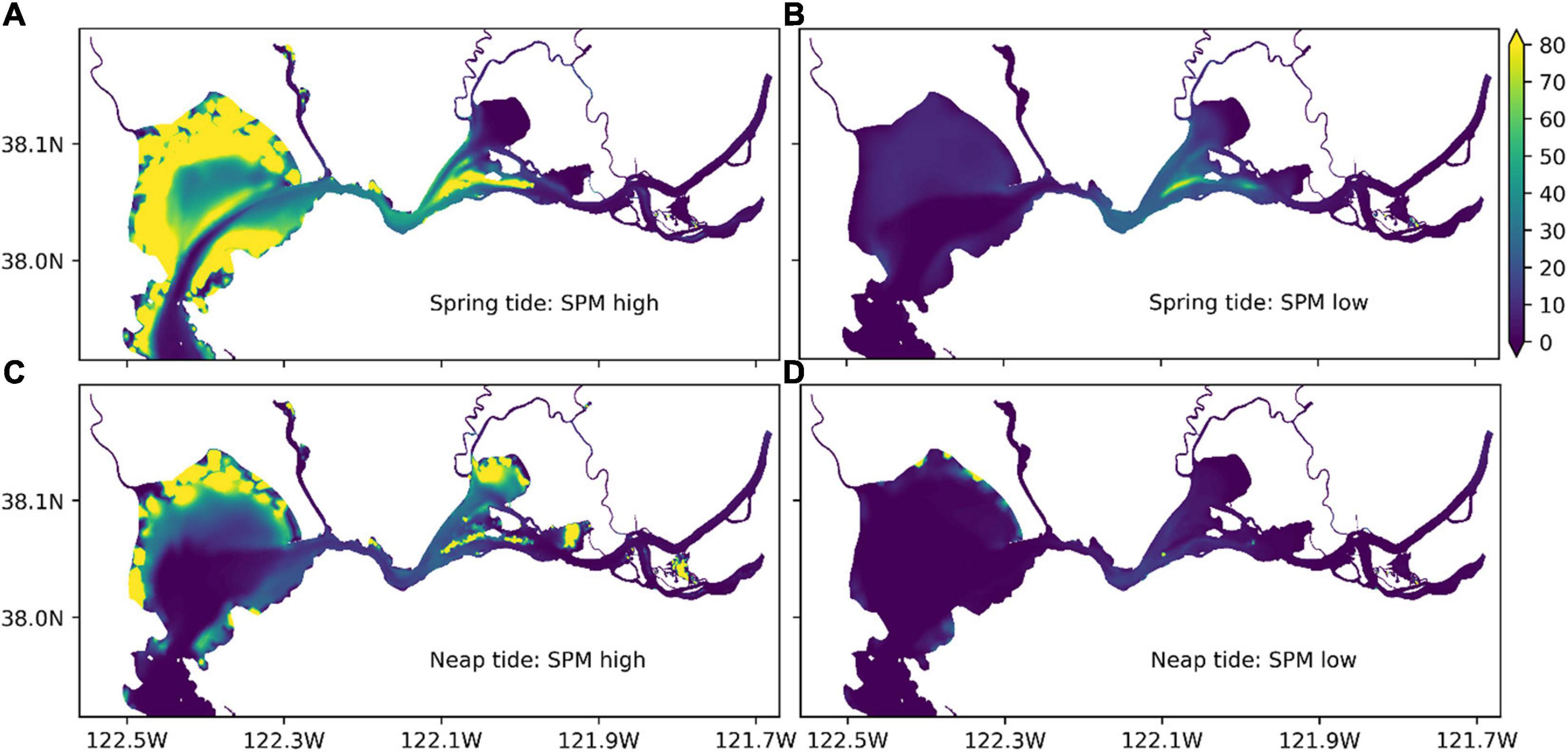
Figure 3. Spatial variation of modeled surface SPM concentration (mg l–1) in northern SFB. The snapshots of high (A,C) and low (B,D) SPMs were taken during spring (April 21 for A and B) and neap (April 27 for C and D) tides.
Figure 4 shows simulated chlorophyll-a concentrations in 2011 at six stations, where monthly chlorophyll-a data measured by the USGS are available (Schraga and Cloern, 2017), using a fixed SPM of 20 mg l–1 and a modeled SPM from SED3D. Note that the simulated chlorophyll-a generated by the model with SPM = 20 mg l–1 is not the same as the chlorophyll-a output in Liu et al. (2018) because different boundary conditions of chlorophyll-a were applied. The chlorophyll-a values from the two runs only show small differences from January to April. This is probably because the influence from large winter–spring river inflow dominated over the influence from local SPM variation (Buchanan and Ganju, 2007; Liu et al., 2018). Thus, the chlorophyll-a pattern in northern SFB during this period can be largely explained by the advection of phytoplankton from north to south. However, noticeable differences in chlorophyll-a concentration between the two simulations can be seen in the second half of the year. Compared to the result of SPM_20, chlorophyll-a in SPM_SED3D presents larger fluctuations, particularly evident at USGS stations 13 and 15 in San Pablo Bay. The chlorophyll-a concentration was higher with many peaks. In July and August, there were larger chlorophyll-a differences between the two simulations at the upstream stations (649, 3, and 6), where chlorophyll-a concentration in SPM_20 was generally less than 3 μg l–1, but chlorophyll-a in SPM_SED3D often exceeded 6 μg l–1. In addition, these larger chlorophyll-a values from SPM_SED3D match observational data better than those in SPM_20. Another difference is that the ecosystem model captures some chlorophyll-a peaks when SED3D was coupled with CoSiNE. For example, there was a phytoplankton bloom in late September when chlorophyll-a concentration exceeded 10 μg l–1. The fully coupled model with SED3D can reproduce this bloom, particularly at stations 9, 13, and 15, while the model with constant SPM concentration completely misses this bloom. The greater fall bloom at stations 13 and 15 was related to the low SPM concentration during that time, while the smaller spring bloom was likely related to the flushing effect from the large river inflow in spring (Liu et al., 2018).
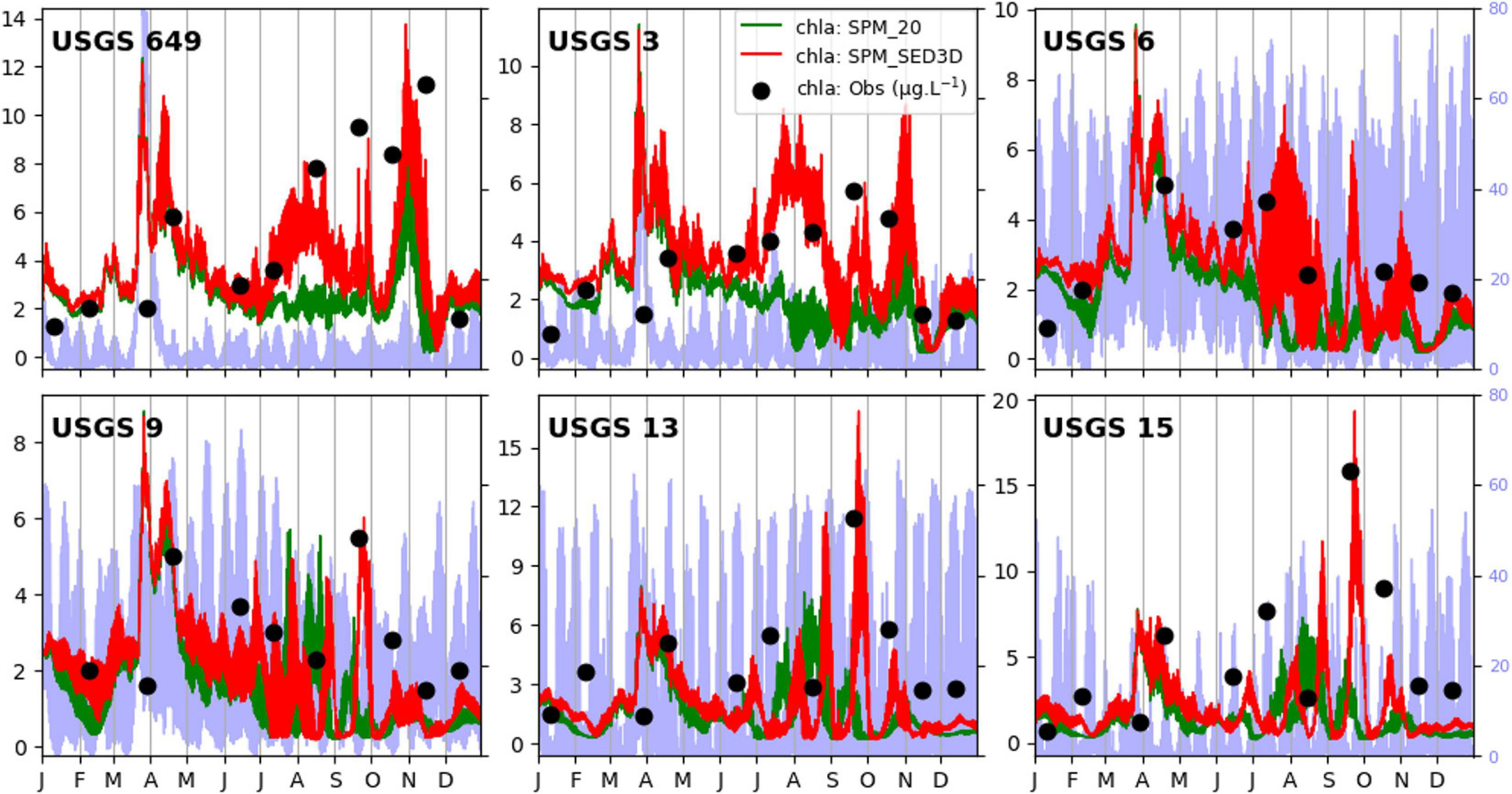
Figure 4. Modeled chlorophyll-a with (red) and without (green) the sediment transport model. The green line is from SPM_20, while the red line is from SPM_SED3D. The dots are measured chlorophyll-a concentrations by the USGS. The light blue line in the background represents the SPM concentration from SPM_SED3D.
A quantitative comparison of chlorophyll-a simulations between SPM_20 and SPM_SED3D is shown in Table 2 (a Taylor diagram is also shown in Figure A2 for reference). For all stations, the model skills for chlorophyll-a in SPM_SED3D are improved to some extent compared to those in SPM_20, more so at stations 649, 13, and 15. It shows that the R of chlorophyll-a in SPM_20 ranges from 0.19 to 0.68, while the R in SPM_SED3D ranges from 0.63 to 0.95 with the maximum value at station 649. The range of MAE of chlorophyll-a in SPM_SED3D is 0.37, 2.11 μg l–1, compared to 0.84, 3.47 μg l–1 in SPM_20. On average, the MAE in SPM_SED3D is reduced by 0.90 μg l–1 (or improved by 48%) relative to that in SPM_20. For ME, the values in SPM_20 are in the range of −2.89, −0.52 μg l–1, which are all negative, suggesting that the model systematically underestimates chlorophyll-a when constant SPM of 20 mg l–1 is used. When the ecosystem model is coupled with SED3D, the ME is improved with a range of −1.49, 0.41 μg l–1, especially at stations 6 and 9 with ME values being 0.04 and 0.05 μg l–1, respectively. The averaged ME in SPM_SED3D is reduced by 0.80 μg l–1 (or improved by 65%).
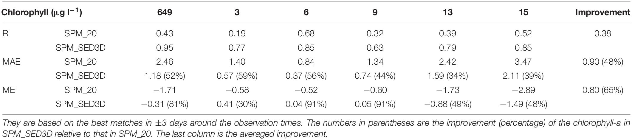
Table 2. Statistics for chlorophyll-a results including R, MAE, and ME for the six stations in northern San Francisco Bay (SFB).
Figure 5 shows the spatial distribution of annual mean surface chlorophyll-a concentration in 2011. The model results match the general pattern obtained from MODIS Aqua satellite data in San Pablo Bay where higher chlorophyll-a concentrations tend to be in shallow water regions and lower chlorophyll-a in deep water regions. The same spatial pattern also appears in Suisun Bay (Figure 5A) where chlorophyll-a concentration is higher along the shallow shoals than in the deep channel. The magnitude of simulated chlorophyll-a concentration seems to be underestimated in comparison with the satellite image in San Pablo Bay with a maximum value about 7 μg l–1 for the model but a maximum value about 12 μg l–1 for the observations. However, it is plausible that the error is associated with the satellite image if we compare the chlorophyll-a values with in situ data (Figure 4). For example, at USGS 13, the average value of in situ chlorophyll-a measurement in 2011 is about 4 μg l–1, but chlorophyll-a value from the satellite image is about 7 μg l–1.
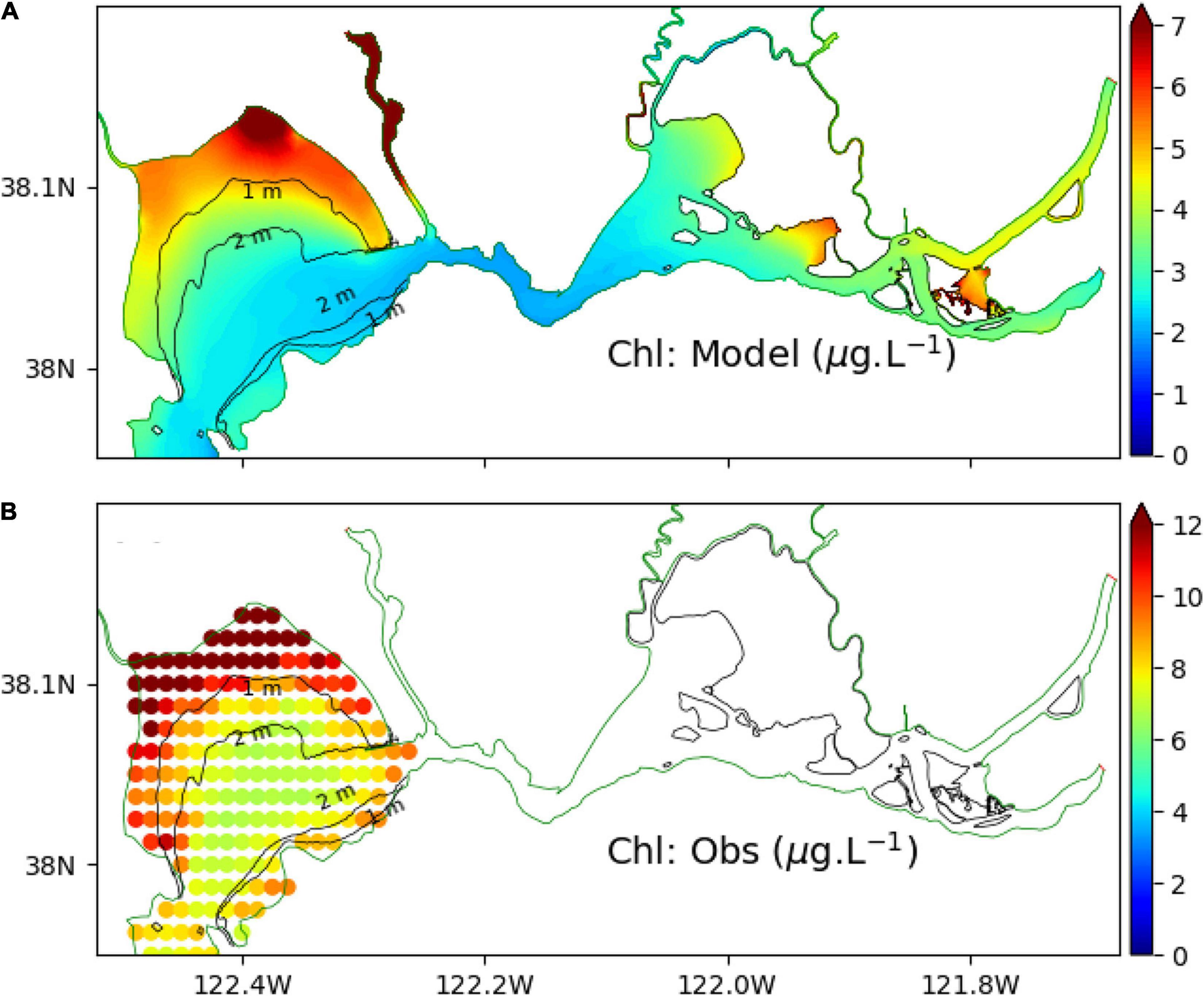
Figure 5. Comparison between modeled surface chlorophyll-a (annually mean in 2011) in SPM_SED3D (A) and data extrapolated from satellite image of chlorophyll-a (B) from MODIS Aqua in SFB (https://coastwatch.pfeg.noaa.gov/erddap/index.html). The satellite data has a resolution of 0.0125 degree. The algorithm in converting wavelengths to chlorophyll-a can be found in Hu et al. (2012) and https://oceancolor.gsfc.nasa.gov/atbd/chlor_a/#sec_2.
Figure 4 shows that the chlorophyll-a simulation was improved when a 3D sediment transport model was incorporated into the ecosystem model. This illustrates the importance of turbidity (or SPM) on phytoplankton dynamics in SFB (Cloern, 1987). Since SPM concentration is influenced by many factors (Barnard et al., 2013) at different time scales, it can potentially impact chlorophyll-a concentration on both short (semi-diurnal, diurnal, and semi-monthly) and long timescales (seasonal).
Figure 2 shows that SPM in northern SFB had diurnal and semi-monthly cycles, consistent with previous findings (Cloern, 1996; Martin et al., 2007; Schoellhamer et al., 2008). In Figure 6, three prominent frequencies are evident: semi-monthly, diurnal, and semi-diurnal. The semi-monthly variation is caused by the spring–neap tidal cycle (Bever and MacWilliams, 2013). The diurnal variation of SPM is largely due to the diurnal tide (Schoellhamer et al., 2008) as well as semi-diurnal tide (Stanev et al., 2007), while the diurnal variation of chlorophyll-a is related to the diurnal variations of light condition and tide (Catts et al., 1985; Powell et al., 1989; Cloern, 1996). Specifically, tidal advection (Conomos, 1979) moves chlorophyll-a patches (as well as SPM) back and forth and can potentially induce daily variation of local chlorophyll-a concentration observed at fixed stations. The diurnal signal of chlorophyll-a variation is also related to the diurnal variation of the light condition, which is in turn caused by the diurnal cycles of both solar radiation and SPM. Because tidal phase is changing with time, tide can be in and out of phase with the variation of light intensity related to the sun movement (Martin et al., 2007; Chen et al., 2010). In addition, SPM varies both in the horizontal and in the vertical, contributing more spatial variation to the light field. Therefore, the spatial and temporal variations are intertwined, which complicates the phytoplankton dynamics in the estuary. The semi-diurnal signal is also included in the time series of SPM and chlorophyll-a, which is likely related to semi-diurnal tide (Cloern, 1996). The semi-diurnal amplitudes of chlorophyll-a and SPM are generally smaller than the diurnal and semi-monthly amplitudes (Figure 6). Overall, the frequency analysis results in Figure 6 show that the coupled model results are consistent with the observations in representing the three dominant cycles of chlorophyll-a and SPM. Similar features between chlorophyll-a and SPM in Figure 6 suggest that besides the light, tide is another major driving forcing in affecting chlorophyll-a variation in northern SFB by regulating the SPM variation. For the subtidal variation of chlorophyll-a, it is also related to river influence, wind, and temperature, apart from the tide/light influence (Cloern et al., 2005; Chen et al., 2010).
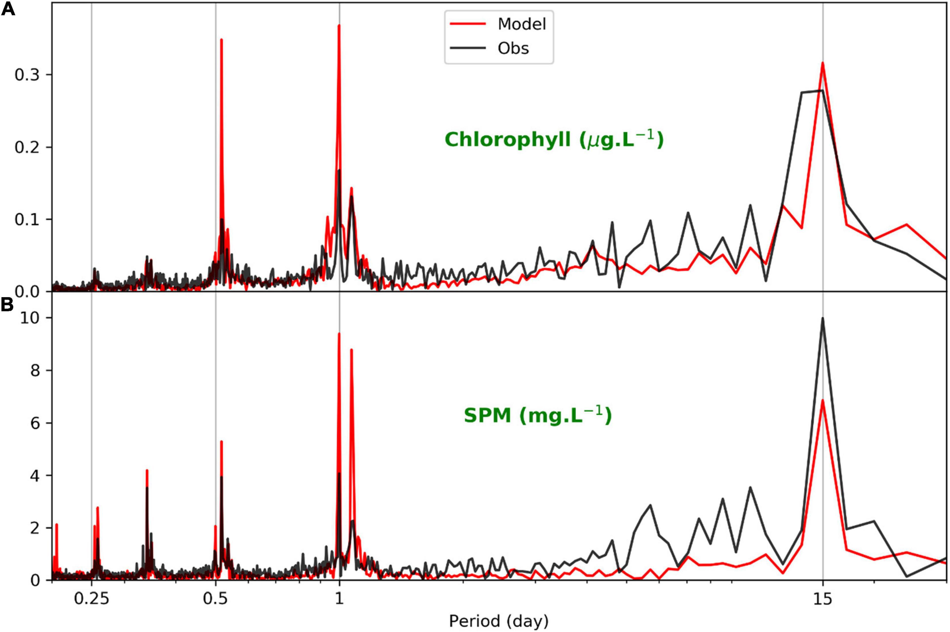
Figure 6. Frequencies of near-surface chlorophyll and SPM at station MRZ based on modeled chlorophyll-a and the Department of Water Resources (DWR) chlorophyll data (A) and based on modeled SPM and DWR turbidity data (B).
In estuarine ecosystem, vertically averaged parameters and vertically integrated parameters are both meaningful to assess the concentrations and budgets of constituents, respectively. Here, we evaluate how light influences these two aspects by focusing on how changing light field affects chlorophyll-a (vertically averaged) and primary productivity (vertically averaged or integrated)–the rate that produces the phytoplankton biomass. The role of the light field is first analyzed. Then, we compared the variations of chlorophyll-a and primary productivity in SFB as well as their relations with the light field.
Figure 7A shows the time series of daily mean Ze at station EZ, which is located in San Pablo Bay with a mean water depth of 1.29 m (Figure 1). Ze obtained using model version SPM_20 is generally deeper than Ze that is determined with the coupled model SPM_SED3D, suggesting that the average SPM concentration from SED3D is greater than 20 mg l–1 at this location. The higher SPM concentration may be caused by wind- or tide-induced sediment resuspension, which substantially increases the SPM concentration in the water column in a shallow water area (Schoellhamer et al., 2008). The average Ze at EZ is about 1.3 m in both runs (Figure 7A), indicating that the entire water column at this location is euphotic because of its shallowness. This is further shown by the increased depth of Ze in late March when a large river inflow (Liu et al., 2018) brought fresh water and increased the water depth in San Pablo Bay. Figure 7B shows the daily mean Ze at USGS 13 where the mean water depth is 9.42 m. In contrast to Ze at station EZ, Ze at USGS 13 in SPM_SED3D is much deeper than that in SPM_20 (which is nearly a constant of about 2 m). The Ze in SPM_SED3D can vary from 2 to 5 m. It shows a strong semi-monthly fluctuation, which is related to the variation of SPM concentration in the surface water modulated by the spring–neap tidal cycle (Buchanan and Ganju, 2007). Moreover, a large drop of Ze occurred at USGS 13 in late March, in contrast to the increase of Ze at station EZ under high river inflow condition. These differences of Ze between shallow and deep locations indicate that Ze values in areas with different water depths have different controlling mechanisms.
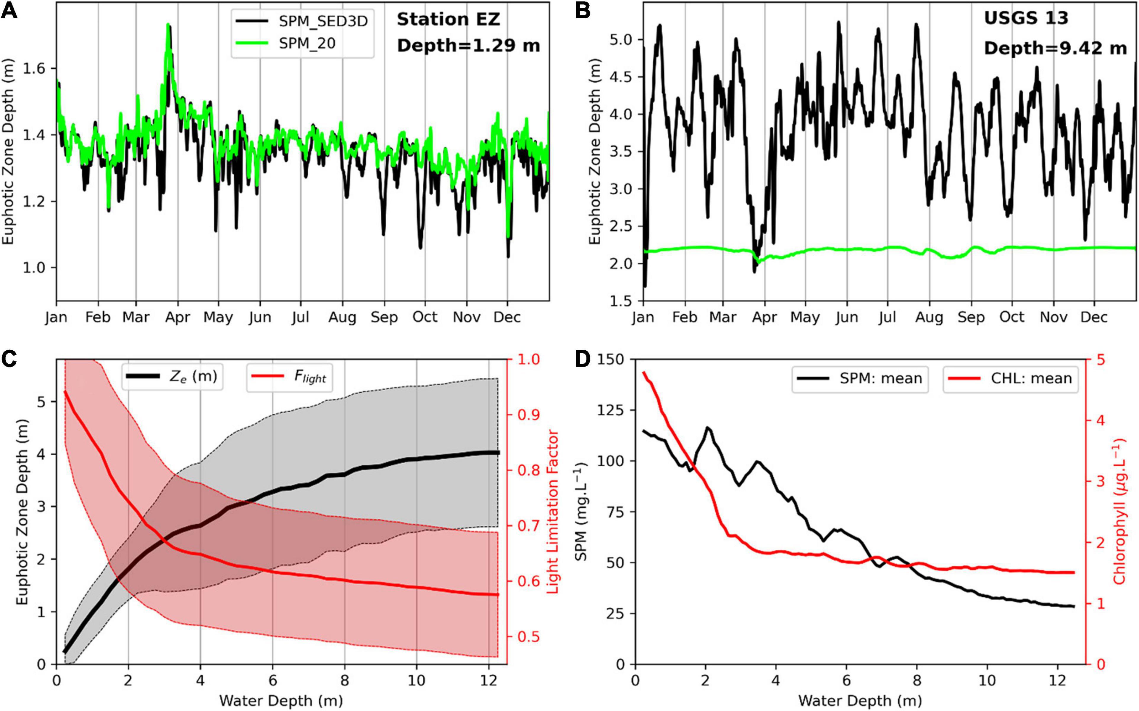
Figure 7. Daily mean euphotic zone depth (Ze) at station EZ (A) and USGS 13 (B) from SPM_20 (green line) and SPM_SED3D (black line). (C) The averaged Ze (black line) and averaged light limitation Flight (red line) in the euphotic zone with standard deviations as shaded areas versus water depth along a transect in San Pablo Bay (Figure 1). Note that Flight was computed using noontime data when solar radiation is the strongest. (D) Averaged surface SPM and surface chlorophyll-a from simulation SED3D versus water depth along the same transect as Ze and Flight.
Figure 7C shows averaged Ze in SPM_SED3D versus water depth along a transect in San Pablo Bay (see Figure 1 for the location) and the standard deviation of Ze. Ze generally increases with water depth. When water depth is less than 2 m, such as at station EZ, Ze increases almost linearly with water depth, suggesting that Ze is generally limited by water depth in the shallow water area. Because of the shallowness, the entire water column is euphotic as shown in Figure 7A. Therefore, the large SPM concentration in shallow water regions (Figure 7D) has a limited effect on Ze and its standard deviation. Instead, when water depth is less than 2 m, the variation of Ze generally follows the tidal variation of water depth. When water depth is more than 2 m, but less than 4 m, Ze also increases with water depth, which means that water depth still plays an important role in determining Ze. In the meantime, the standard deviation of Ze begins to increase with water depth. This may indicate that the SPM variation in the water column has started to affect Ze because the water column is not completely euphotic, and light penetration in SFB is related to SPM concentration in the bay (Cloern, 1987). When water depth is larger than 4 m, Ze increases less with water depth, and the standard deviation does not change much. This means that in deep water regions, water depth has no major control on Ze. Instead, the variation of Ze is primarily due to the SPM variation in the surface water. Figure 7C also shows Flight versus water depth along the same transect for Ze in San Pablo Bay. Unlike Ze that increases with water depth, Flight decreases steeply when water depth is less than 4 m, and then decreases gently when water depth is larger than 4 m. As Flight represents the overall light limitation, its variation with depth in Figure 7C means that phytoplankton growth is less light limited in shallow water regions than in deep water regions, which is consistent with the conclusion of Bukaveckas et al. (2011) that shallow water regions are generally not light limited.
Figure 7D shows averaged surface SPM concentration and chlorophyll-a versus water depth. Generally, averaged SPM concentration decreases with water depth. At shallow depth (<4 m), surface SPM concentration is around 75–100 mg l–1 associated with a large variation, as it is close to the bottom where sediment can be resuspended. In deep water regions (>4 m), the averaged SPM concentration changes from ∼80 to ∼25 mg l–1 when water depth increases from 4 to 12 m. If we regard the typical mean chlorophyll-a = 3 μg/l and SPM = 50 mg/l, their contributions ( and ) to light attenuation are −0.09 and −3.3, respectively. Therefore, SPM plays a major role in affecting the light field in SFB. The variation of SPM at different water depths may be related to different mechanisms in sediment resuspension. Wind can disturb the bottom and substantially modify the SPM concentration in shallow water, but its influence cannot penetrate into deep water (Schoellhamer et al., 2008). Tides can resuspend the bottom sediment in deep water region and redistribute SPM in the water column (Bever and MacWilliams, 2013). This difference results in a higher SPM concentration in the shallow water region than that in the deep water region. The decreasing trend in SPM concentration with water depth in Figure 7D is consistent with the variation of Ze with water depth in Figure 7C. However, the high SPM concentration in the shallow water region of San Pablo Bay did not cause light limitation on phytoplankton growth (Figure 7C). This is suggested by a higher chlorophyll-a concentration in the shallow water regions (<3 m, Figure 7D) with averaged chlorophyll-a decreasing from above 4.5 to below 2.0 μg l–1 with water depth. In the deep water regions (>3 m), averaged chlorophyll-a has a range of [1.5, 2.0] μg l–1.
Chlorophyll-a concentration represents the accumulation of phytoplankton growth minus the reduction from all loss terms including predation, respiration, mortality, and sinking (Chai et al., 2002; Cerco and Noel, 2004). Primary productivity represents the rate of carbon increase over time that is a growth term of phytoplankton, which is affected by many factors, including nutrients, light, and temperature (Kemp and Boynton, 1984; Marshall and Nesius, 1996; Dugdale et al., 2013). In this study, we regard that PP serves as a proxy of phytoplankton growth. To investigate how the light availability related to SPM can influence phytoplankton dynamics in SFB, we show the vertical distribution of chlorophyll-a concentration and PP at USGS station 13 during 2011 for both simulations in Figure 8. One prominent feature of chlorophyll-a concentration is that it is largely well-mixed in the water column, compared to PP that peaks near the surface. Strong seasonal variation in PP occurs with a spring peak in March–April in both runs, a fall peak in July–August in SPM_20, and several peaks in August–September in SPM_SED3D. During winter, PP remains low. PP is the strongest at the water surface, but decreases rapidly with depth. PP in SPM_20 is restricted to the top 1–2 m, while PP in SPM_SED3D can extend to depths as great as 5 m. There exists substantial short-term variability of PP in SPM_SED3D compared to that in SPM_20. Figure 8D shows strong semi-monthly fluctuation of PP, which corresponds to the variation of Ze in Figure 7B. It suggests that the spring–neap tidal cycle can greatly affect PP by influencing the SPM concentration in the surface water. The different vertical structures between chlorophyll-a concentration and PP are due to different processes affecting these two parameters. Phytoplankton growth only happens in the euphotic zone. Thus, PP is restricted to the upper part of water column. However, phytoplankton cells can be vertically mixed throughout the water column, resulting in very small difference between surface and bottom chlorophyll-a concentrations in SFB and leading to the homogenous distributions seen in Figures 8A,C.
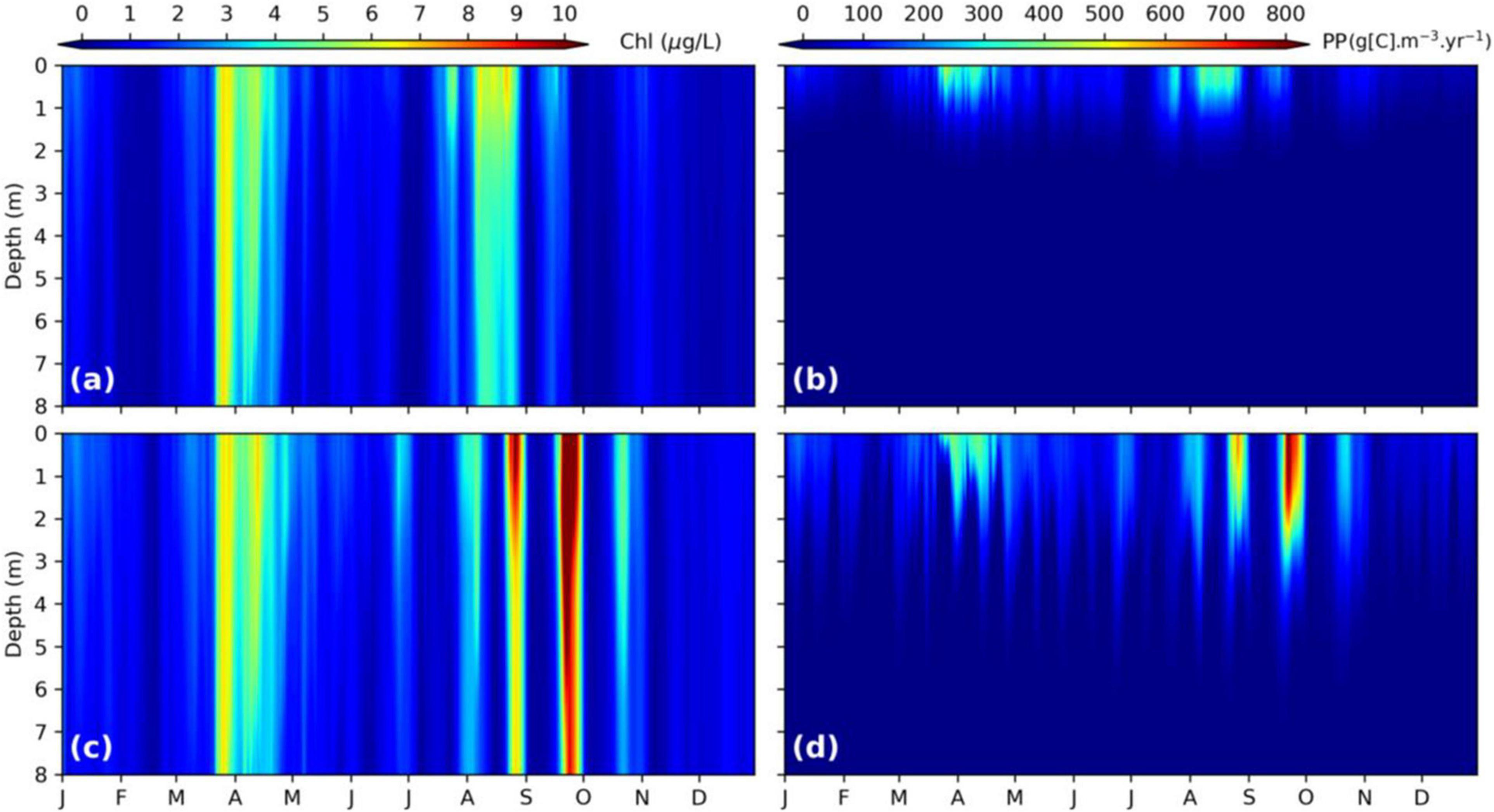
Figure 8. Noontime chlorophyll-a concentration (A,C) and primary productivity (B,D) varying with depth and time at station USGS 13. The top panel is from SPM_20, while the bottom panel is from SPM_SED3D.
The similar variations with water depth for Flight in Figure 7C and for chlorophyll-a in Figure 7D suggest that Flight may be a good indicator of chlorophyll-a concentration in SFB. To investigate this, we computed Flight (Figure 9A) and vertically averaged chlorophyll-a (Figure 9B) and PP (Figure 9C) in northern SFB. In Figure 9A, high values of Flight (>0.8) are mainly in the shallow water regions (water depth < 2 m) of San Pablo Bay and Suisun Bay. Along the deep channels, Flight has lower values and can drop to 0.5. The averaged chlorophyll-a in the euphotic zone in Figure 9B shows a horizontal distribution similar to that of Flight. High chlorophyll-a concentrations (>4 μg l–1) are also distributed in the shallow water area (water depth < 2 m), and chlorophyll-a values larger than 6 μg l–1 are mostly located near the margin of San Pablo Bay, where water depth is less than 1 m. Toward the deeper region (water depth > 2 m), chlorophyll-a is low, especially along the channels where chlorophyll-a can drop below 2 μg l–1. In Figure 9C, it shows that vertically averaged PP has the same features as chlorophyll-a in the spatial distribution (thus, also similar to Flight), although PP has different vertical structures (Figure 8). The comparison among Flight, chlorophyll-a, and PP in Figure 9 suggests that Flight can be used to describe the averaged light limitation on phytoplankton growth in northern SFB. Flight is higher in shallow water regions than in deep water regions, suggesting that phytoplankton growth in shallow water areas is less limited by light, which results in higher chlorophyll-a concentration in the euphotic zone.
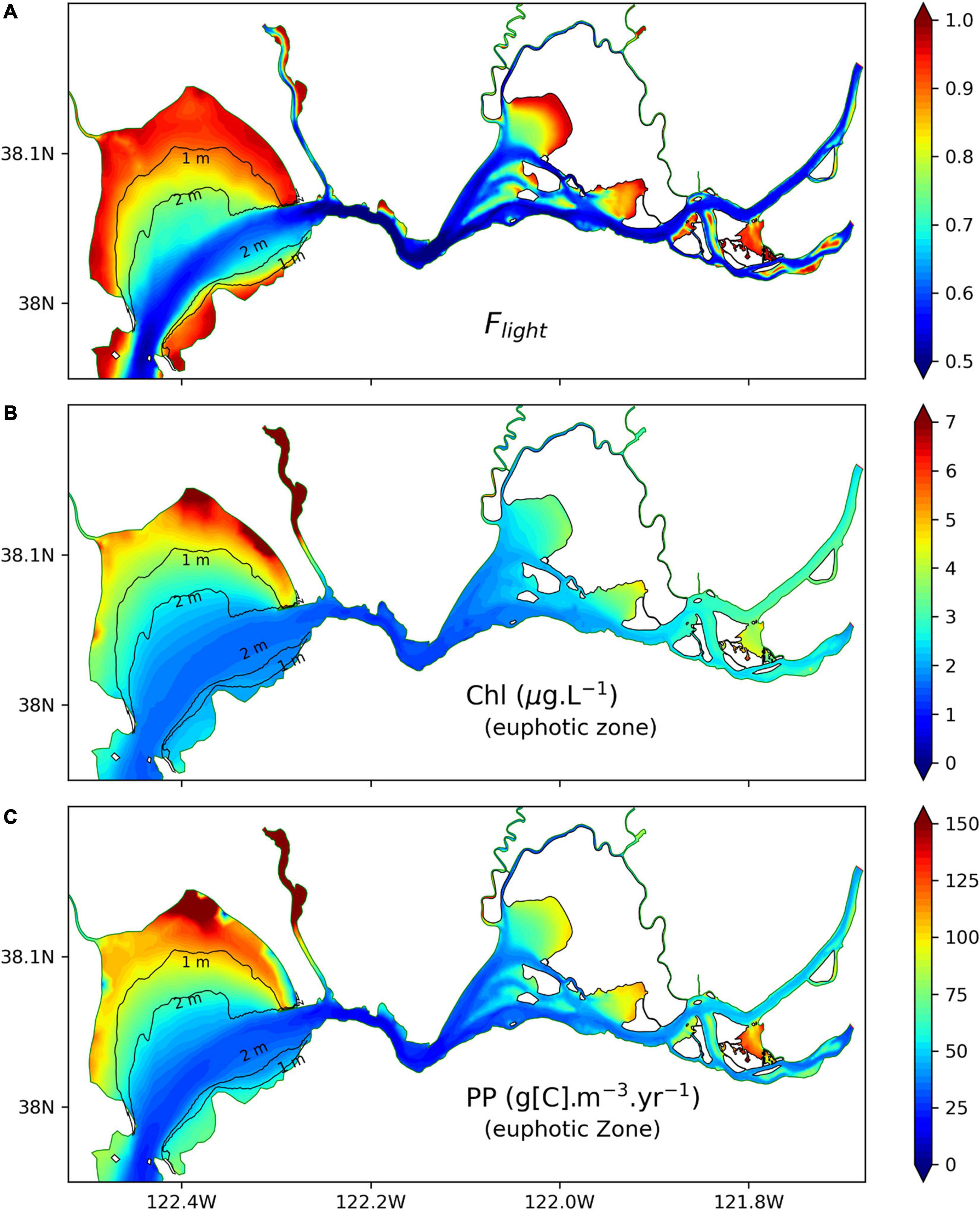
Figure 9. (A) Light limitation factor Flight at noontime in northern SFB, (B) vertically averaged chlorophyll-a concentration in the euphotic zone at noontime, and (C) vertically averaged PP in the euphotic zone at noontime. All the data are from SPM_SED3D and are temporally averaged for 2011. Contour lines show 1- and 2-m bathymetry in San Pablo Bay.
Figure 10 displays annual mean Ze in northern SFB in 2011 as well as vertically integrated PP. Note that PP here is different from the vertically averaged PP in Figure 9. It shows that vertically integrated PP is low (high) in shallow (deep) water region, which is consistent with the small (large) Ze (Figure 10A) in the shallow (deep) water region. Therefore, Ze serves as a good indicator for the vertically integrated PP in northern SFB. The spatial distribution of Ze and PP in Figure 10 is consistent with our analysis of Ze at different water depths in Figure 7. In the shallow water regions, Ze is largely constrained by water depth, although SPM concentration in SPM_SED3D can vary greatly. In contrast, in the deep water regions, to a large extent, Ze is determined by SPM concentration in the surface water. In Figure 10B, the annual mean PP in northern SFB can vary from below 30 to over 180 g[C] m–2 year–1 in different areas. Cole and Cloern (1984) measured PP at multiple locations in SFB. Their values of annual mean PP were 140–160 g[C] m–2 year–1 in San Pablo Bay and 110–120 g[C] m–2 year–1 in Suisun Bay. Jassby et al. (2002) calculated the PP based upon chlorophyll-a and light penetration in the bay delta region and reported an averaged PP of 70 g[C] m–2 year–1, with a variation over a factor of five in different years. Recently, Wilkerson et al. (2015) measured the annual PP in Suisun Bay to be 40–60 g[C] m–2 year–1 in 2011 and 2012, and Kimmerer et al. (2012) reported a smaller PP of 25–31 g[C] m–2 year–1 in 2006 and 2007 in SFB. In general, our estimated PP is consistent with those reported values that fall in the range of PP in Figure 10B.
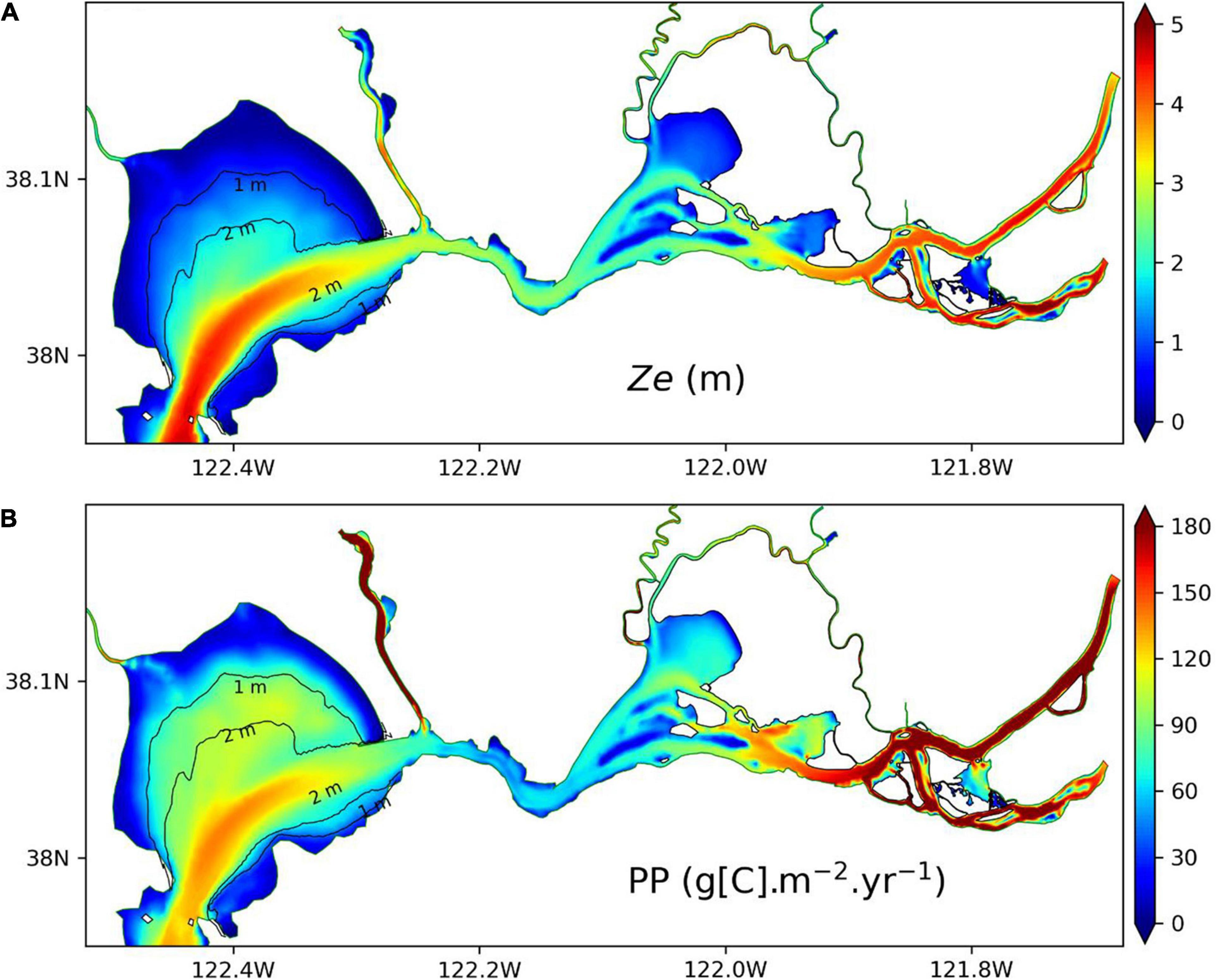
Figure 10. Comparison of euphotic zone depth (A) and vertically integrated primary productivity (B) in northern SFB for 2011. All the data are from SPM_SED3D.
However, the spatial distribution of Ze is opposite to the distribution of Flight that shows large (small) values in shallow (deep) water regions (Figure 9). As Ze is an indicator for vertically integrated PP and Flight is an indicator for vertically averaged chlorophyll-a and PP, correspoindingly, vertically integrated PP presents an inversed spatial pattern of vertically averaged chlorophyll-a and PP. The vertically integrated PP represents the accumulation of phytoplankton growth integrated in the euphotic zone; thus, it is mainly controlled by Ze. The low PP rates in shallow water areas are kept low, mainly due to small Ze, even though the average phytoplankton concentration is higher (Figure 7D), while the large PP in deep water region is due to large Ze with greater amount of water column for growth. On the other hand, the vertically averaged chlorophyll-a concentration and PP in Figure 9 represent the mean strength of phytoplankton growth in the euphotic zone, which is related to the mean light availability in the euphotic zone, as represented by Flight. This leads to similar spatial distributions shared by Flight and chlorophyll-a concentration. Although the SPM concentration in northern SFB is relatively higher in shallow water region than in deep water region, it does not cause light limitation on phytoplankton growth in the shallow water region, likely because the SPM concentration is not high enough to completely block the light penetration. Therefore, chlorophyll-a concentration can be high in the shallow water areas. In the deep water areas, lower SPM concentration (Figure 7D) means a larger Ze. The light factor ϕ(z) (see Eq. 1) may change with depth, from one at the surface to a rather low value at the depth of Ze, which may result in a small Flight for the euphotic zone. This explains the lower chlorophyll-a concentrations in the deep water regions compared to the shallow water regions of northern SFB. The significance of Ze and Flight is that they can be roughly estimated by using SPM because light attenuation is dominated by SPM in SFB (Cloern, 1987; Buchanan and Ganju, 2007), which provides another way to assess the ecosystem without resorting to calculating or tracking all the complex biogeochemical processes.
Figure 11 shows monthly mean PP that is averaged over northern SFB. For all months, PP resulting from using SPM_20 is lower than that with SPM_SED3D; the latter varied from 40.4 g[C] m–2 year–1 in December to 140.6 g[C] m–2 year–1 in September. The two peaks of PP in April and August–September in Figure 11 correspond to the spring and fall blooms in Figure 8, respectively. In addition, the underestimated PP in SPM_20 is intensified in the winter months. For example, in December, the PP in SPM_20 (14.2 g[C] m–2 year–1) is only 35% of the PP in SPM_SED3D (40.4 g[C] m–2 year–1). Therefore, the incorporation of SED3D into CoSiNE not only improved the chlorophyll-a time series at individual stations (Figure 4) but also increased the bay-wide PP estimate.
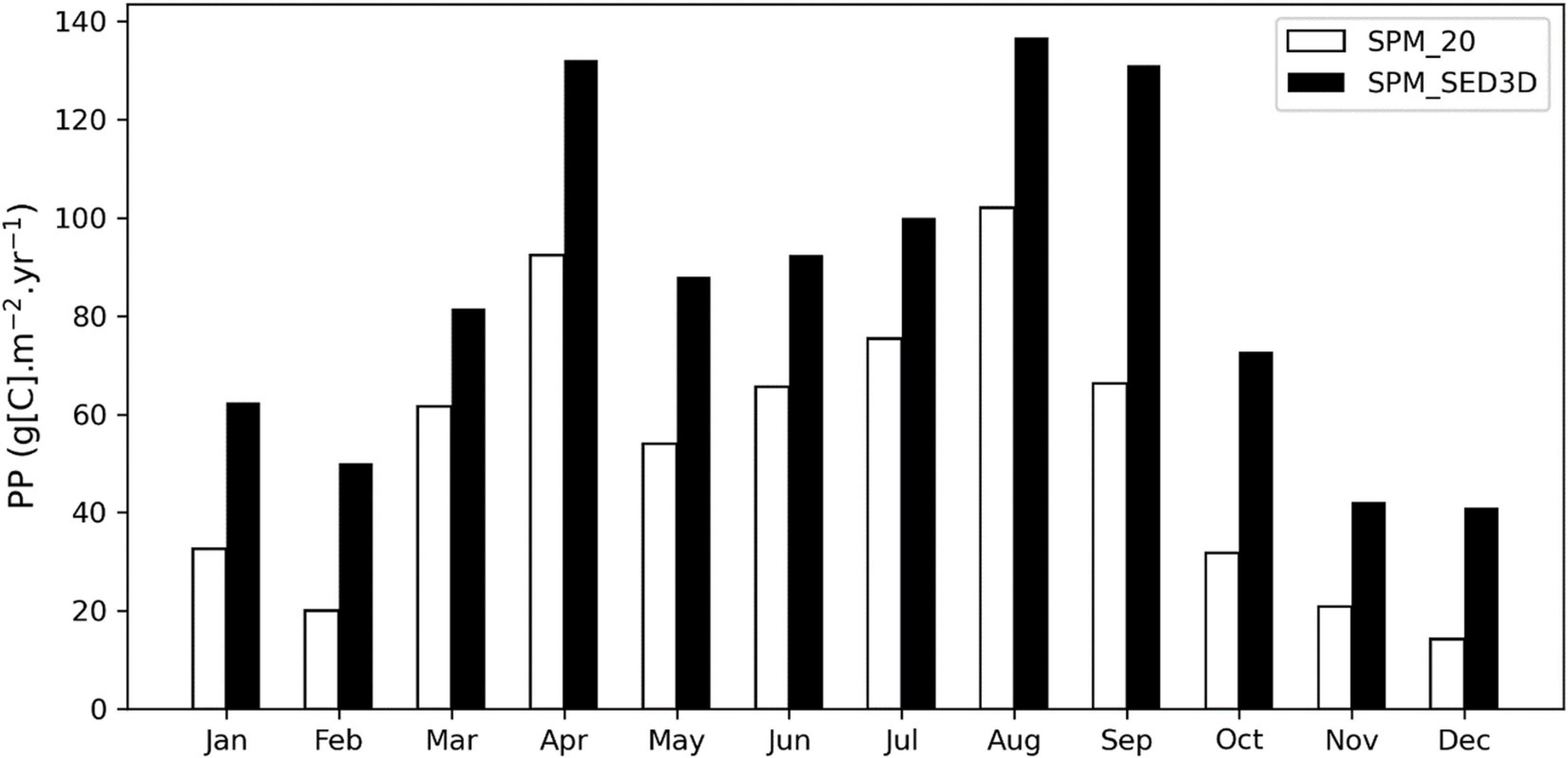
Figure 11. Comparison of monthly mean primary productivity between SPM_20 and SPM_SED3D simulations.
In this study, we developed a three-way coupled modeling system, including a hydrodynamic model (SCHISM), a biogeochemical model (CoSiNE), and a sediment transport model (SED3D), to investigate the effect of irradiance as determined by SPM on phytoplankton growth in northern SFB. The SPM simulated by SED3D was used for computing light conditions that were used in the biogeochemical CoSiNE model. We focused on how SPM in the water column influences light penetration and subsequent phytoplankton growth. We calculated euphotic zone depth (Ze) and defined a new parameter “averaged light limitation” (Flight) that vertically integrates the photosynthetic light factor through the euphotic zone.
The summary of the findings of this study are as follows:
(a) The sediment model SED3D was able to simulate SPM concentration well in northern SFB at semi-diurnal, diurnal, and semi-monthly time scales and cycles. Chlorophyll-a simulation produced by the CoSiNE model is more realistic when it is coupled to SED3D compared to the simulation with SPM set to a constant value of 20 mg l–1.
(b) Ze in shallow water regions (<2 m) was shown to be determined by water depth, while Ze in deep water regions is controlled by SPM concentration in the whole water column. Ze appears to be a good indicator for vertically integrated primary productivity that varies from 40 to 160 g[C] m–2 year–1 at different locations.
(c) Flight appears to be a good indicator of vertically averaged chlorophyll-a and PP. The averaged chlorophyll-a concentration follows a similar distribution of Flight with high (low) values in shallow (deep) water regions.
Our study demonstrates the importance of SPM determining light availability for phytoplankton growth in northern SFB and the need to include sediment models in ecosystem simulations. It also shows that both SPM and chlorophyll-a concentration are strongly modulated by spring–neap tidal cycle. More importantly, these results suggest the advantage of coupling a sediment transport model and a biogeochemical model in simulating spatial and temporal variation of ecosystem dynamics in northern SFB. We highlight that euphotic zone depth (Ze) and “averaged light limitation” (Flight) analyzed in this study can be useful physical indicators of biogeochemical variables in systems with similar morphometric characteristics of SFB.
The raw data supporting the conclusions of this article will be made available by the authors, without undue reservation.
ZW: conducting the model simulation, collecting the data, performing the data analysis, writing the manuscript, and proposing the research methods and ideas. FC and HX: supervising research progress, proposing research methods, proposing research ideas, and editing manuscript. YZ, XW, RD, and FW: proposing research methods and editing manuscript. All authors contributed to the article and approved the submitted version.
This study is supported by the DOE project “Improving tide-estuary representation in MPAS-Ocean” (Grant Number DE-SC0016263 to YZ at the Virginia Institute of Marine Sciences) and by the California Department of Fish and Wildlife through funding for RD and FW (Q1996035) at San Francisco State University and for FC (subaward S20-0004) at the University of Maine.
The authors declare that the research was conducted in the absence of any commercial or financial relationships that could be construed as a potential conflict of interest.
Babin, M., Stramski, D., Ferrari, G. M., Claustre, H., Bricaud, A., Obolensky, G., et al. (2003). Variations in the light absorption coefficients of phytoplankton, nonalgal particles, and dissolved organic matter in coastal waters around Europe. J. Geophys. Res. 108:3211. doi: 10.1029/2001JC000882
Barnard, P. L., Schoellhamer, D. H., Jaffe, B. E., and McKee, L. J. (2013). Sediment transport in the San Francisco Bay coastal system: an overview. Mar. Geol. 345, 3–17. doi: 10.1016/j.margeo.2013.04.005
Bever, A. J., and MacWilliams, M. L. (2013). Simulating sediment transport processes in San Pablo Bay using coupled hydrodynamic, wave, and sediment transport models. Mar. Geol. 345, 235–253. doi: 10.1016/j.margeo.2013.06.012
Buchanan, P. A., and Ganju, N. K. (2007). Summary of suspended-sediment concentration data, San Francisco Bay, California, water year 2005. U. S. Geol. Surv. Data Ser. 282:46.
Bukaveckas, P. A., Barry, L. E., Beckwith, M. J., David, V., and Lederer, B. (2011). Factors determining the location of the chlorophyll maximum and the fate of algal production within the Tidal Freshwater James River. Estuaries Coasts 34, 569–582. doi: 10.1007/s12237-010-9372-4
Catts, G. P., Khorram, S., Cloern, J. E., Knight, A. W., and Degloria, S. D. (1985). Remote sensing of tidal chlorophyll-a variations in estuaries. Int. J. Remote Sens. 6, 1685–1706. doi: 10.1080/01431168508948318
Cerco, C. F., and Noel, M. R. (2004). The 2002 Chesapeake Bay Eutrophication Model. Annapolis, MD: U.S. Environmental Protection Agency.
Chai, F., Dugdale, R. C., Peng, T. H., Wilkerson, F. P., and Barber, R. T. (2002). One-dimensional ecosystem model of the equatorial Pacific upwelling system. Part I: model development and silicon and nitrogen cycle. Deep Sea Res. II Top. Stud. Oceanogr. 49, 2713–2745. doi: 10.1016/s0967-0645(02)00055-3
Chai, F., Jiang, M. S., Chao, Y., Dugdale, R. C., Chavez, F., and Barber, R. T. (2007). Modeling responses of diatom productivity and biogenic silica export to iron enrichment in the equatorial Pacific Ocean. Glob. Biogeochem. Cycles 21:16. doi: 10.1029/2006gb002804
Chao, Y., Farrara, J. D., Zhang, H., Zhang, Y. J., Ateljevich, E., Chai, F., et al. (2017). Development, implementation, and validation of a modeling system for the San Francisco Bay and estuary. Estuar. Coast. Shelf Sci. 194, 40–56. doi: 10.1016/j.ecss.2017.06.005
Chen, Z., Hu, C., Muller-Karger, F. E., and Luther, M. E. (2010). Short-term variability of suspended sediment and phytoplankton in Tampa Bay, Florida: observations from a coastal oceanographic tower and ocean color satellites. Estuar. Coast. Shelf Sci. 89, 62–72. doi: 10.1016/j.ecss.2010.05.014
Cloern, J. E. (1987). Turbidity as a control on phytoplankton biomass and productivity in estuaries. Cont. Shelf Res. 7, 1367–1381. doi: 10.1016/0278-4343(87)90042-2
Cloern, J. E. (1996). Phytoplankton bloom dynamics in coastal ecosystems: a review with some general lessons from sustained investigation of San Francisco Bay, California. Rev. Geophys. 34, 127–168. doi: 10.1029/96rg00986
Cloern, J. E. (2001). Our evolving conceptual model of the coastal eutrophication problem. Mar. Ecol. Prog. Ser. 210, 223–253. doi: 10.3354/meps210223
Cloern, J. E., and Jassby, A. D. (2012). Drivers of change in estuarine-coastal ecosystems: discoveries from four decades of study in San Francisco Bay. Rev. Geophys. 50:33. doi: 10.1029/2012rg000397
Cloern, J. E., and Nichols, F. H. (1985). “Time scales and mechanisms of estuarine variability, a synthesis from studies of San Francisco Bay,” in Temporal Dynamics of an Estuary: San Francisco Bay, eds J. E. Cloern and F. H. Nichols (Dordrecht: Springer), 229–237. doi: 10.1007/978-94-009-5528-8_14
Cloern, J. E., Hieb, K. A., Jacobson, T., Sanso, B., Di Lorenzo, E., Stacey, M. T., et al. (2010). Biological communities in San Francisco Bay track large-scale climate forcing over the North Pacific. Geophys. Res. Lett. 37:6. doi: 10.1029/2010gl044774
Cloern, J. E., Schraga, T. S., Lopez, C. B., Knowles, N., Labiosa, R. G., and Dugdale, R. (2005). Climate anomalies generate an exceptional dinoflagellate bloom in San Francisco Bay. Geophys. Res. Lett. 32:5. doi: 10.1029/2005gl023321
Cole, B. E., and Cloern, J. E. (1984). Significance of biomass and light availability to phytoplankton productivity in San Francisco Bay. Mar. Ecol. Prog. Ser. 17, 15–24. doi: 10.3354/meps017015
Conomos, T. (1979). “Properties and circulation of San Francisco Bay waters,” in San Francisco Bay–The Urbanized Estuary, ed. T. J. Conomos (San Francisco, CA: Pacific Division, American Association for the Advancement of Science), 47–84.
Conomos, T., Smith, R., and Gartner, J. (1985). “Environmental setting of San Francisco Bay,” in Temporal Dynamics of An Estuary: San Francisco Bay, eds J. E. Cloern and F. H. Nichols (Dordrecht: Springer), 1–12. doi: 10.1007/978-94-009-5528-8_1
Doyle, J. D., Jiang, Q., Chao, Y., and Farrara, J. (2009). High-resolution real-time modeling of the marine atmospheric boundary layer in support of the AOSN-II field campaign. Deep Sea Res. II Top. Stud. Oceanogr. 56, 87–99. doi: 10.1016/j.dsr2.2008.08.009
Dugdale, R. C., Wilkerson, F. P., and Parker, A. E. (2013). A biogeochemical model of phytoplankton productivity in an urban estuary: the importance of ammonium and freshwater flow. Ecol. Modell. 263, 291–307. doi: 10.1016/j.ecolmodel.2013.05.015
Dugdale, R. C., Wilkerson, F. P., and Parker, A. E. (2016). The effect of clam grazing on phytoplankton spring blooms in the low-salinity zone of the San Francisco estuary: a modelling approach. Ecol. Modell. 340, 1–16. doi: 10.1016/j.ecolmodel.2016.08.018
Dugdale, R., Wilkerson, F., Parker, A. E., Marchi, A., and Taberski, K. (2012). River flow and ammonium discharge determine spring phytoplankton blooms in an urbanized estuary. Estuar. Coast. Shelf Sci. 115, 187–199. doi: 10.1016/j.ecss.2012.08.025
Elias, E. P., and Hansen, J. E. (2013). Understanding processes controlling sediment transports at the mouth of a highly energetic inlet system (San Francisco Bay, CA). Mar. Geol. 345, 207–220. doi: 10.1016/j.margeo.2012.07.003
Fichot, C. G., Downing, B. D., Bergamaschi, B. A., Windham-Myers, L., Marvin-DiPasquale, M., Thompson, D. R., et al. (2016). High-resolution remote sensing of water quality in the San Francisco Bay–delta estuary. Environ. Sci. Technol. 50, 573–583. doi: 10.1021/acs.est.5b03518
Hu, C., Lee, Z., and Franz, B. (2012). Chlorophyll aalgorithms for oligotrophic oceans: a novel approach based on three-band reflectance difference. J. Geophys. Res. 117:C01011. doi: 10.1029/2011JC007395
Jassby, A. D., Cloern, J. E., and Cole, B. E. (2002). Annual primary production: patterns and mechanisms of change in a nutrient-rich tidal ecosystem. Limnol. Oceanogr. 47, 698–712. doi: 10.4319/lo.2002.47.3.0698
Kemp, W. M., and Boynton, W. R. (1984). Spatial and temporal coupling of nutrient inputs to estuarine primary production – the role of particulate transport and decomposition. Bull. Mar. Sci. 35, 522–535.
Kimmerer, W. J., Parker, A. E., Lidström, U. E., and Carpenter, E. J. (2012). Short-term and interannual variability in primary production in the low-salinity zone of the San Francisco estuary. Estuaries Coasts 35, 913–929. doi: 10.1007/s12237-012-9482-2
Liu, Q., Chai, F., Dugdale, R., Chao, Y., Xue, H., Rao, S., et al. (2018). San Francisco Bay nutrients and plankton dynamics as simulated by a coupled hydrodynamic-ecosystem model. Cont. Shelf Res. 161, 29–48. doi: 10.1016/j.csr.2018.03.008
Lucas, L. V., Cloern, J. E., Thompson, J. K., Stacey, M. T., and Koseff, J. R. (2016). Bivalve grazing can shape phytoplankton communities. Front. Mar. Sci. 3:14. doi: 10.3389/fmars.2016.00014
Lucas, L. V., Thompson, J. K., and Brown, L. R. (2009). Why are diverse relationships observed between phytoplankton biomass and transport time? Limnol. Oceanogr. 54, 381–390. doi: 10.4319/lo.2009.54.1.0381
Marshall, H., and Nesius, K. (1996). Phytoplankton composition in relation to primary production in Chesapeake Bay. Mar. Biol. 125, 611–617.
Martin, M. A., Fram, J. P., and Stacey, M. T. (2007). Seasonal chlorophyll a fluxes between the coastal Pacific Ocean and San Francisco Bay. Mar. Ecol. Prog. Ser. 337, 51–61. doi: 10.3354/meps337051
Muylaert, K., Tackx, M., and Vyverman, W. (2005). Phytoplankton growth rates in the freshwater tidal reaches of the Schelde estuary (Belgium) estimated using a simple light-limited primary production model. Hydrobiologia 540, 127–140. doi: 10.1007/s10750-004-7128-5
Novick, E., and Senn, D. (2014). External Nutrient Loads to San Francisco Bay. SFEI Contribution No. 704. Richmond, CA: San Francisco Estuary Institute.
Pinto, L., Fortunato, A., Zhang, Y., Oliveira, A., and Sancho, F. (2012). Development and validation of a three-dimensional morphodynamic modelling system for non-cohesive sediments. Ocean Model. 57, 1–14. doi: 10.1016/j.ocemod.2012.08.005
Platt, T., Gallegos, C., and Harrison, W. G. (1980). Photoinhibition of photosynthesis in natural assemblages of marine phytoplankton. J. Mar. Res. 38, 687–701.
Platt, T., Harrison, W., Irwin, B., Horne, E. P., and Gallegos, C. L. (1982). Photosynthesis and photoadaptation of marine phytoplankton in the Arctic. Deep Sea Res. A Oceanogr. Res. Pap. 29, 1159–1170. doi: 10.1016/0198-0149(82)90087-5
Powell, T. M., Cloern, J. E., and Huzzey, L. M. (1989). Spatial and temporal variability in South San Francisco Bay (USA). I. Horizontal distributions of salinity, suspended sediments, and phytoplankton biomass and productivity. Estuar. Coast. Shelf Sci. 28, 583–597. doi: 10.1016/0272-7714(89)90048-6
Schoellhamer, D. H., Ganju, N. K., and Shellenbarger, G. G. (2008). “Sediment transport in San Pablo Bay,” in Technical Studies for the Aquatic Transfer Facility: Hamilton Wetlands Restoration Project: Chapter 2, Final Draft Technical Report, eds D. A. Cacchione and P. A. Mull (San Francisco, CA: U.S. Army Corps of Engineers), 36–107.
Schoellhamer, D. H., Wright, S. A., and Drexler, J. (2012). A conceptual model of sedimentation in the Sacramento–San Joaquin Delta. San Franc. Estuary Watershed Sci. 10. Available online at: https://escholarship.org/uc/item/2652z8sq
Schraga, T. S., and Cloern, J. E. (2017). Water quality measurements in San Francisco Bay by the US Geological Survey, 1969–2015. Sci. Data 4:170098.
Sellner, K. G., Doucette, G. J., and Kirkpatrick, G. J. (2003). Harmful algal blooms: causes, impacts and detection. J. Ind. Microbiol. Biotechnol. 30, 383–406. doi: 10.1007/s10295-003-0074-9
Sommer, T., Armor, C., Baxter, R., Breuer, R., Brown, L., Chotkowski, M., et al. (2007). The collapse of pelagic fishes in the upper San Francisco Estuary: El colapso de los peces pelagicos en la cabecera del Estuario San Francisco. Fisheries 32, 270–277. doi: 10.1577/1548-8446(2007)32[270:tcopfi]2.0.co;2
Stanev, E., Brink-Spalink, G., and Wolff, J. O. (2007). Sediment dynamics in tidally dominated environments controlled by transport and turbulence: a case study for the East Frisian Wadden Sea. J. Geophys. Res. 112:C04018. doi: 10.1029/2005JC003045
U.S. Geological Survey Data (2018). National Water Information System Data Available on the World Wide Web (USGS Water Data for the Nation).Available online at: https://waterwatch.usgs.gov (accessed June 10, 2018).
U.S. Geological Survey (2014). Water-Resources Data for the United States, Water Year 2013: U.S. Geological Survey Water-Data Report WDR-US-2013, Site 11447650. Availble online at: http://wdr.water.usgs.gov/wy2013/pdfs/11447650.2013.pdf (accessed February 18, 2021).
Wang, Z., Chai, F., Dugdale, R., Liu, Q., Xue, H., Wilkerson, F., et al. (2020). The interannual variabilities of chlorophyll and nutrients in San Francisco Bay: a modeling study. Ocean Dyn. 70, 1169–1186. doi: 10.1007/s10236-020-01386-0
Wang, Z., Wang, H., Shen, J., Ye, F., Zhang, Y., Chai, F., et al. (2019). An analytical phytoplankton model and its application in the tidal freshwater James River. Estuar. Coast. Shelf Sci. 224, 228–244. doi: 10.1016/j.ecss.2019.04.051
Warnock, S. E., and Takekawa, J. Y. (1995). Habitat preferences of wintering shorebirds in a temporally changing environment: western Sandpipers in the San Francisco Bay estuary. Auk 112, 920–930. doi: 10.2307/4089023
Wilkerson, F. P., Dugdale, R. C., Parker, A. E., Blaser, S. B., and Pimenta, A. (2015). Nutrient uptake and primary productivity in an urban estuary: using rate measurements to evaluate phytoplankton response to different hydrological and nutrient conditions. Aquat. Ecol. 49, 211–233. doi: 10.1007/s10452-015-9516-5
Zhang, Y., and Baptista, A. M. (2008). SELFE: a semi-implicit Eulerian-Lagrangian finite-element model for cross-scale ocean circulation. Ocean Model. 21, 71–96. doi: 10.1016/j.ocemod.2007.11.005
Zhang, Y., Ye, F., Stanev, E. V., and Grashorn, S. (2016). Seamless cross-scale modeling with SCHISM. Ocean Model. 102, 64–81. doi: 10.1016/j.ocemod.2016.05.002
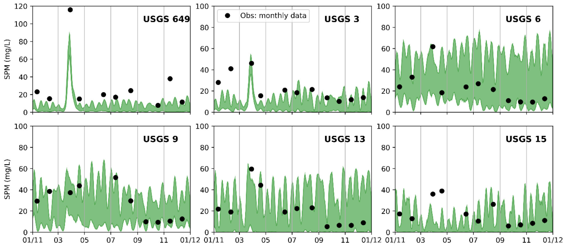
Figure A1. Daily ranges of simulated surface SPM concentrations (mg l–1) compared with monthly observations at six USGS stations.
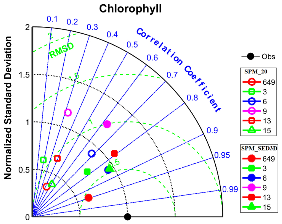
Figure A2. Taylor diagram for chlorophyll-a simulations at six USGS stations in northern SFB. Markers with solid color are for SPM_SED3D, while open markers are for SPM_20. In this figure, each variable is normalized by the standard deviation of its corresponding observed field.
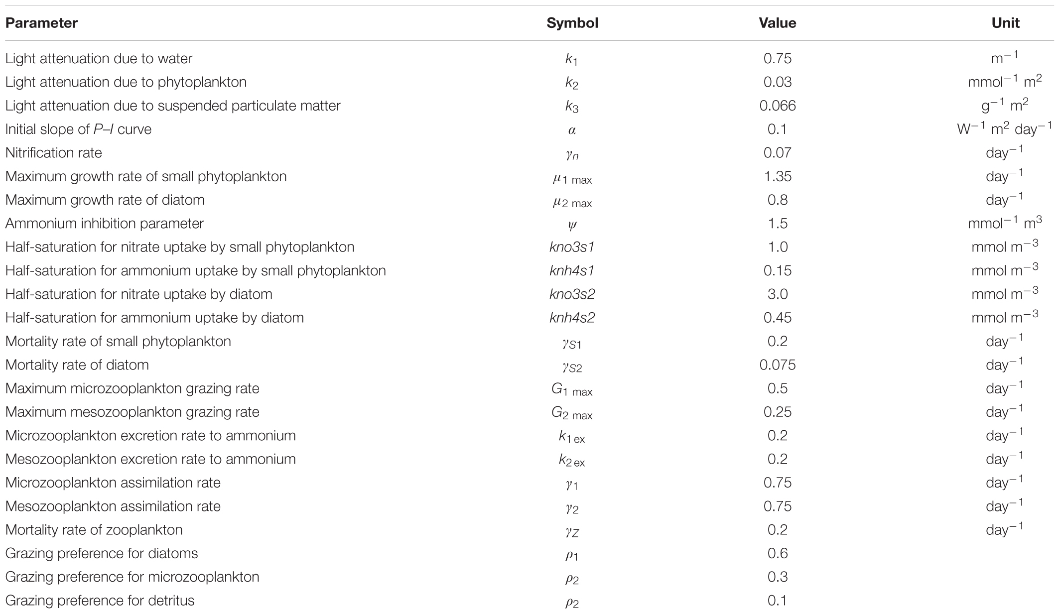
Table A1. CoSiNE model parameter and values.
Keywords: light availability, phytoplankton growth, SPM, sediment transport model, CoSiNE, SCHSIM
Citation: Wang Z, Chai F, Xue H, Wang XH, Zhang YJ, Dugdale R and Wilkerson F (2021) Light Regulation of Phytoplankton Growth in San Francisco Bay Studied Using a 3D Sediment Transport Model. Front. Mar. Sci. 8:633707. doi: 10.3389/fmars.2021.633707
Received: 18 February 2021; Accepted: 28 May 2021;
Published: 25 June 2021.
Edited by:
Alejandro Jose Souza, Center for Research and Advanced Studies–Mérida Unit, MexicoReviewed by:
José Pinho, University of Minho, PortugalCopyright © 2021 Wang, Chai, Xue, Wang, Zhang, Dugdale and Wilkerson. This is an open-access article distributed under the terms of the Creative Commons Attribution License (CC BY). The use, distribution or reproduction in other forums is permitted, provided the original author(s) and the copyright owner(s) are credited and that the original publication in this journal is cited, in accordance with accepted academic practice. No use, distribution or reproduction is permitted which does not comply with these terms.
*Correspondence: Fei Chai, ZmNoYWlAbWFpbmUuZWR1
Disclaimer: All claims expressed in this article are solely those of the authors and do not necessarily represent those of their affiliated organizations, or those of the publisher, the editors and the reviewers. Any product that may be evaluated in this article or claim that may be made by its manufacturer is not guaranteed or endorsed by the publisher.
Research integrity at Frontiers
Learn more about the work of our research integrity team to safeguard the quality of each article we publish.