A Novel Framework to Predict Relative Habitat Selection in Aquatic Systems: Applying Machine Learning and Resource Selection Functions to Acoustic Telemetry Data From Multiple Shark Species

Griffin, Lucas P.; Casselberry, Grace A.; Hart, Kristen M.; Jordaan, Adrian; Becker, Sarah L.; Novak, Ashleigh J.; DeAngelis, Bryan M.; Pollock, Clayton G.; Lundgren, Ian; Hillis-Starr, Zandy; Danylchuk, Andy J.; Skomal, Gregory B.

doi:10.3389/fmars.2021.631262

ORIGINAL RESEARCH article

Front. Mar. Sci., 29 April 2021

Sec. Marine Ecosystem Ecology

Volume 8 - 2021 | https://doi.org/10.3389/fmars.2021.631262

This article is part of the Research Topic Habitat and Distribution Models of Marine and Estuarine Species: Advances for a Sustainable Future View all 15 articles

A Novel Framework to Predict Relative Habitat Selection in Aquatic Systems: Applying Machine Learning and Resource Selection Functions to Acoustic Telemetry Data From Multiple Shark Species

$\r\nLucas P. Griffin*$ Lucas P. Griffin^1*

Grace A. Casselberry¹

Ashleigh J. Novak¹

Ian Lundgren⁵

Zandy Hillis-Starr⁶

Andy J. Danylchuk^1†

Gregory B. Skomal^7†

¹Department of Environmental Conservation, University of Massachusetts Amherst, Amherst, MA, United States
²Wetland and Aquatic Research Center, United States Geological Survey, Davie, FL, United States
³The Nature Conservancy, Narragansett, RI, United States
⁴National Park Service, Key West, FL, United States
⁵Office of Habitat Conservation, NOAA Fisheries, Silver Spring, MD, United States
⁶National Park Service, Christiansted, US Virgin Islands
⁷Massachusetts Division of Marine Fisheries, New Bedford, MA, United States

Resource selection functions (RSFs) have been widely applied to animal tracking data to examine relative habitat selection and to help guide management and conservation strategies. While readily used in terrestrial ecology, RSFs have yet to be extensively used within marine systems. As acoustic telemetry continues to be a pervasive approach within marine environments, incorporation of RSFs can provide new insights to help prioritize habitat protection and restoration to meet conservation goals. To overcome statistical hurdles and achieve high prediction accuracy, machine learning algorithms could be paired with RSFs to predict relative habitat selection for a species within and even outside the monitoring range of acoustic receiver arrays, making this a valuable tool for marine ecologists and resource managers. Here, we apply RSFs using machine learning to an acoustic telemetry dataset of four shark species to explore and predict species-specific habitat selection within a marine protected area. In addition, we also apply this RSF-machine learning approach to investigate predator-prey relationships by comparing and averaging tiger shark relative selection values with the relative selection values derived for eight potential prey-species. We provide methodological considerations along with a framework and flexible approach to apply RSFs with machine learning algorithms to acoustic telemetry data and suggest marine ecologists and resource managers consider adopting such tools to help guide both conservation and management strategies.

Introduction

Habitat loss and degradation are two of the largest drivers of loss in global biodiversity (Hoekstra et al., 2005), making identifying important habitats critical for resource managers to prioritize habitat protection for species of concern (Morris and Kingston, 2002; Chetkiewicz and Boyce, 2009; Heinrichs et al., 2017). Habitat selection is driven by the physical, chemical, and biological composition and condition of an area that is occupied by a given animal (Block and Brennan, 1993). Thus, behavioral choices related to selection are ultimately determined by a wide range of coupled and uncoupled abiotic and biotic factors, such as energetic demands and tradeoffs from foraging opportunities, predation risk, and competition (Rosenzweig, 1974; Craig and Crowder, 2002). Understanding how species select habitats across heterogeneous landscapes provides key information regarding occupancy patterns that contribute to survival and reproductive success (Kramer et al., 1997; McGarigal et al., 2016). Such information could then be used to identify, protect, and restore specific ecologically valuable habitats and corridors (Kramer and Chapman, 1999; Beier et al., 2008; Fraschetti et al., 2009; Zeller et al., 2017).

Resource selection functions (RSFs), defined as a function that produces values that are proportional to the probability of use by an animal (Manly et al., 2007), are a popular method to determine and predict relative habitat selection by animals (e.g., Nielsen et al., 2003; Johnson et al., 2004; Ciarniello et al., 2007). These functions evaluate the relationships between resource use (i.e., the units of area selected by an animal) and the environmental characteristics associated with each unit of area (Boyce et al., 2002). Animal spatial data, from sources such as telemetry, can be incorporated into RSFs to define the relative habitat selection strengths among animal space use and a given set of environmental covariates, such as habitat type, substrate, elevation, or water depth (Boyce and McDonald, 1999). When the true absences are unknown, as generated by presence only data derived from sources such as telemetry approaches, RSFs are implemented within a use/availability framework where known presences (1) are compared with a random sample across ‘available’ resource units, also known as pseudo-absences or background points (0) (Boyce, 2006; Pearce and Boyce, 2006). Alternative to use/availability (e.g., from telemetry), data from observations collected from survey methods, often without timestamps, are typically referred to as presence-background and are fitted as species distribution models (Fieberg et al., 2018). Using RSFs to derive the relative probability of selection, rather than the absolute probability (see Lele et al., 2013; Avgar et al., 2017), telemetry data are then typically fitted using logistic regression models (Johnson et al., 2006; Manly et al., 2007) or, as of more recently, with machine learning algorithms [e.g., random forest (RF), boosted regression trees] (Shoemaker et al., 2018; Heffelfinger et al., 2020).

While RSFs have been largely applied in terrestrial ecology, such as with wolves (Ordiz et al., 2020), birds (Meager et al., 2012), grizzly bears (McLoughlin et al., 2002), and deer (Godvik et al., 2009), the application of RSFs within aquatic environments has been limited comparatively, likely due to technological challenges related to continuously tracking animals through water (Hussey et al., 2015). Today, passive acoustic telemetry has become one of the most common practices to quantify aquatic animal space use (Cooke et al., 2004; Donaldson et al., 2014; Hussey et al., 2015). This technique involves tagging an animal with an acoustic transmitter that periodically emits an ultrasonic ping with a unique identification number (ID code). When in range and with sufficient detection efficiency the ping is detected by an acoustic receiver that registers both the unique ID code and the time the transmitter was detected (Hussey et al., 2015). Depending on the scope and extent of both research questions and available funding, acoustic receivers are strategically arranged in fixed locations with either non-overlapping detection ranges (Heupel et al., 2006; Brownscombe et al., 2019b), or with overlapping detection ranges that can produce high resolution positioning estimates of space use (Espinoza et al., 2011). While both methods are limited to the available detection coverage (presence only data), the former is often used to examine space use across a given study area at much larger spatial extents (Carlisle et al., 2019) and, thus, is well catered to exploring relative habitat selection.

Although the application of RSFs in combination with acoustic telemetry has been limited (see Freitas et al., 2016; Harrison et al., 2016; Gutowsky et al., 2017; Selby et al., 2019; Griffin et al., 2020), much needed information on animal habitat selection in the marine environment can be derived. For example, Selby et al. (2019) and Griffin et al. (2020) applied RSFs to acoustic telemetry data for hawksbill (Eretmochelys imbricata) and juvenile green turtle (Chelonia mydas), respectively, from St. Croix, United States Virgin Islands, and determined that the size and extent of a marine protected area (MPA) being used by these sea turtles was sufficient to meet conservation goals. In addition to providing insights on potential drivers of relative habitat selection, RSFs were also extended to predict movements in areas that did not have acoustic receivers to provide potential locations where fine-scale habitat protection may be further prioritized (Griffin et al., 2020). Such results have important implications within marine environments especially for resource managers seeking to incorporate animal movement data to generate effective conservation strategies (Cooke, 2008; Knip et al., 2012; Allen and Singh, 2016; Hays et al., 2016, 2019; Lea et al., 2016). Since management and conservation efforts often rely on spatial management techniques (Peel and Lloyd, 2004; Sequeira et al., 2019), including MPAs (Gell and Roberts, 2003; Lubchenco et al., 2003; Gleason et al., 2010; Lubchenco and Grorud-Colvert, 2015; Weeks et al., 2017; Feeley et al., 2018; Keller et al., 2020; Gallagher et al., 2021), habitat selection predictions should help managers meet conservation endpoints and play a role in evaluating management alternative strategies for both species and for the habitats on which they rely on.

In this study, we provide a framework to implement RSFs using machine learning algorithms to examine and accurately predict relative habitat selection for tracking data collected using acoustic telemetry. Specifically, we apply RSFs to evaluate the relative habitat and resource selection of four shark species: Caribbean reef (Carcharhinus perezi), lemon (Negaprion brevirostris), nurse (Ginglymostoma cirratum), and tiger (Galeocerdo cuvier) sharks within a Caribbean MPA. In the Caribbean Sea, these four species occupy a wide range of environments from nearshore reef and seagrass habitats to offshore pelagic habitats (Pikitch et al., 2005; Legare et al., 2015; Pickard et al., 2016; Casselberry et al., 2020; Gallagher et al., 2021). Considering Caribbean reef sharks are listed as “Endangered” by the IUCN Red List (Carlson et al., 2021a), lemon and nurse sharks are listed as “Vulnerable” (Carlson et al., 2021b, c), and tiger sharks are listed as “Near Threatened” (Ferreira and Simpfendorfer, 2019), all with decreasing population trends, conservation and management efforts would benefit from understanding and incorporating findings surrounding their spatial ecology.

Successful management is especially needed since it has been suggested losses in shark abundance may disrupt food web dynamics that would lead to reduced ecosystem health (Baum and Worm, 2009; Ferretti et al., 2010; Heupel et al., 2014; Hammerschlag et al., 2019). Indeed, food web simulations for Caribbean coral reefs show sharks, as top predators, are members of strongly interacting tri-trophic food chains whose loss could result in trophic cascades (Bascompte et al., 2005). This is supported by in situ studies of mesopredator fish populations in Australia that found shark-depleted coral reefs have reduced fish diversity, species abundance, and biomass, with individual species showing changes in diet and body condition when compared to reefs with healthy shark populations (Barley et al., 2017a, b). Information about shark habitat use and selection could lead to proactive management strategies to mitigate non-sustainable or illegal harvest (White et al., 2017; Jacoby et al., 2020) and/or protect and restore important habitat (Speed et al., 2016; Daly et al., 2018). Because spatial management techniques, such as MPAs, can provide protection for multiple species across a variety of life stages, understanding resource selection across species should help to tailor effective conservation strategies and, specifically, ensure adequate coverage of ecologically vital habitats and areas (Lea et al., 2016).

Considering MPA design may benefit from the inclusion and understanding of predator-prey dynamics (Micheli et al., 2004; Cashion et al., 2020), we also demonstrate how RSFs can be extended to examine spatially explicit relationships between marine predators and their prey. This was accomplished by deriving and averaging overlapping selection values from tiger sharks and from their potential prey, including juvenile green turtles, juvenile Caribbean reef sharks, juvenile lemon sharks, great barracuda (Sphyraena barracuda), horse-eye jack (Caranx latus), yellowtail snapper (Ocyurus chrysurus), and mutton snapper (Lutjanus analis) (Lowe et al., 1996; Simpfendorfer et al., 2001; O’Shea et al., 2015; Aines et al., 2018; Gallagher et al., 2021). Herein, we provide a framework for studies wishing to investigate animal relative habitat selection and predator-prey relationships with acoustic telemetry in marine environments.

Ultimately, these collective RSF findings provide insights into shark spatial ecology and is useful for the conservation of Caribbean reef, lemon, nurse, and tiger sharks and their habitats. In addition, we have included an R code vignette (Appendix A), to improve accessibility and application of RSFs and machine learning.

Materials and Methods

Study Area and Field Data Collection

Buck Island Reef National Monument (BIRNM), a 77 km² no-take MPA, is located on the northeast shelf of St. Croix, United States Virgin Islands (Pittman et al., 2008). Buck Island is an uninhabited, 0.7 km² island that is situated in the middle of the MPA, and 2.5 km northeast of St. Croix. This MPA ranges from shallow-water habitats (<10 m) near the island to deep-water habitats (>1,000 m) off the continental shelf. Generally, benthic habitats range from lagoon habitat (50–150 m wide, around the island excluding the west and southwest sides of the island), linear reef (south side of island and wrapping toward northwest corner), patch reef systems (northwest and north of the island, and south of the southern linear reef), seagrass patches (Thalassia sp., Syringodium sp., and Halophila sp.) and sand flats (south and southwest) (Pittman et al., 2008; Costa et al., 2012).

Between 2011 and 2019, a total of 147 VEMCO VR2W receivers (Innovasea Systems Inc., Nova Scotia, Canada) were deployed as a passive acoustic receiver array within BIRNM to study multiple species (Becker et al., 2016, 2020; Bryan et al., 2019; Selby et al., 2019; Casselberry et al., 2020; Griffin et al., 2020; Novak et al., 2020a, b) (Supplementary). Receivers were deployed, in depths ranging from 2 to 40 m, either on sand screws or cement block anchors around the island with receiver downloads occurring twice a year (see Becker et al., 2016; Selby et al., 2016; Casselberry et al., 2020 for mooring details). Among years, the receiver array design changed in extent through the addition of new receiver stations or decommissioning old stations, due to the availability of receivers and evolving project goals, while maintaining a core set of receiver stations through the duration of the project. The array began with 17 receivers in 2011 and reached its greatest coverage with 147 receivers in 2017. For this study, we collected and analyzed acoustic telemetry data from only 2013–2019 when detection coverage and tag deployment was most substantial across BIRNM. Animal tracking data were collected from surgically implanted V13 or V16 transmitters (delay 60–180 s, battery life 360–3,217 days, Innovasea Systems Inc., Nova Scotia, Canada) in 14 Caribbean reef sharks (between 2013 and 2019), 10 lemon sharks (between 2013 and 2019), 11 nurse sharks (between 2013 and 2019), and eight tiger sharks (between 2015 and 2019). In addition, to examine prey habitat selection in relation to tiger shark selection, data were also collected from 58 juvenile green turtles (between 2013 and 2014), 25 great barracuda (hereinafter referred to as barracuda) (between 2014 and 2015), five horse-eye jack (between 2016 and 2017), eight yellowtail snapper (between 2015 and 2017), and four mutton snapper (between 2015 and 2016). All detection data were reviewed and filtered to remove false detections (Simpfendorfer et al., 2015), including detections that occurred within 60 s of each other for a given individual, singular detections occurring within 12 h, and detections that indicated unrealistic movements (>3 m per second). Tagging locations and methods, including additional specific detection filtering processes, can be found for sharks in Casselberry et al. (2020), barracuda in Becker et al. (2016), horse-eye jack in Novak et al. (2020a), yellowtail snapper in Novak et al. (2020b), and for green turtles in Griffin et al. (2020).

Framework to Apply RSFs Using Acoustic Telemetry and Machine Learning

To derive and predict relative selection values of each species, we describe four important components that include defining available resource units, aggregating habitat information, implementing, evaluating, and interpreting RSFs with machine learning algorithms, and, ultimately, predicting habitat selection for sharks across BIRNM. All analyses were conducted in R version 3.6.2 (R Core Team, 2019). We describe each step in detail below and in the included R code vignette (Appendix A).

Defining Available Resource Units and Presence/Background Points

To estimate fine resolution space use away from the exact location of receivers, detection data was first converted into short-term centers of activity (COAs) using the mean position algorithm (Simpfendorfer et al., 2002). To disaggregate detection data from receiver locations, this method, using the detections across multiple receivers, provides position estimates that are based on the weighted means of the number of detections among each receiver during a specified time window (Simpfendorfer et al., 2002). Here, using the VTRACK package (Campbell et al., 2012), this algorithm was implemented with 90-min time bins to provide animal positioning data across BIRNM (Selby et al., 2019; Griffin et al., 2020). In addition to disaggregating data from receiver locations, constructed COAs provide an approach to potentially reduce issues with autocorrelation by subsampling data into defined time steps (e.g., 90-min bins) (Matley et al., 2017). Autocorrelation, an inherent problem with tracking data, occurs when sequential locations are obtained from the same individual and can lead to biased parameter estimates of animal habitat/space use (Legendre, 1993; Johnson et al., 2013; Fleming et al., 2015).

Consistent with Selby et al. (2019) and Griffin et al. (2020), we defined our available resource units by deriving 400 m buffers around each receiver for each year it was deployed (i.e., 2013–2019) (Supplementary Figure 1). While detection range was variable across BIRNM habitats with an average of 58.2% (95% confidence interval: 44–73% CI) probability of detection at 100 m distance from a receiver (Selby et al., 2016), we decided to extend the buffer size to 400 m since COAs are able to provide approximate positioning estimates even outside of receiver detection range.

To implement RSFs within a use/availability framework and to account for variable receiver coverage across years, we restricted both the COAs (presences) and the randomly distributed background points (pseudo-absences) to our defined available resource units (400 m receiver buffers at the year level) only. Background points were randomly distributed equal to the number of observed COAs (see Barbet-Massin et al., 2012) per individual, diel period (night vs. day), and year across all available resource units (Figure 1). Diel period was calculated using the maptools package (Bivand and Lewin-Koh, 2013). Only using COAs and background points that were within the 400 m buffer from any receiver, they were then collapsed into 200 m × 200 m raster cells.

FIGURE 1

Figure 1. Conceptual diagram to implement resource selection functions with acoustic telemetry and machine learning algorithms; from generated centers of activities and background points, deriving available resource units, model development, model performance and interpretation, and, ultimately, predicting and extrapolating relative selection.

Aggregating Habitat Information

Using habitat mapping data provided by the National Oceanic and Atmospheric Administration (NOAA) (Costa et al., 2012), we converted available and relevant shapefile data into 200 m × 200 m raster cells using the raster (Hijmans et al., 2015) and the sp (Pebesma et al., 2012) packages. Derived habitat raster files included classifications aggregated by zone (fore reef, reef flat, lagoon, etc.) (Supplementary Figure 2A), fine-scale structure (aggregate reef, sand, pavement with sand channels, etc.) (Supplementary Figure 2B), fine-scale cover [seagrass patchy (10%–<50%), seagrass patchy (50–<90%), seagrass continuous (90–100%), etc.], broad-scale cover (algae, live coral, seagrass, etc.), and percent coral cover (i.e., 0–<10%, 10–<50%). In addition, we generated two relevant habitat raster files including distance to land (m) (Buck Island) and depth (m) (Supplementary Figure 3).

Subsequently, corresponding habitat and depth information were extracted from each raster cell and assigned to each COA and background point using the rasterize function from the raster package (Hijmans et al., 2015) (see Appendix A). Habitat information was converted into factors with depth (m) and distance to land (m) remaining as continuous variables.

Applying RSFs With Machine Learning

Resource selection functions were applied using RF models, a commonly utilized machine learning algorithm, to evaluate the relative habitat selection of each species within BIRNM. RF, using binary recursive partitioning to fit multiple data trees with randomly selected predictor subsets (Breiman, 2001), effectively reduces variance and model overfitting while optimizing predictive accuracy (James et al., 2013; Hengl et al., 2018; Schratz et al., 2018). To increase the prediction of the response variable (presences/background points), RF models were fit for each species with 500 trees, replacement, and with 60% of the data. The 40% remainder of each dataset, known as the holdout dataset, were then used to test model performance. RF models were implemented in the ranger (Wright and Ziegler, 2015) and mlr (Bischl et al., 2016) packages.

Characteristic of RF models, a user may tune how trees are generated and fitted from the data. These controls, referred to as hyperparameters, are set prior to fitting an RF by running multiple iterations of values (see Probst et al., 2019). While default values for hyperparameters lead to relatively high performance alone, tuning can often lead to overall model improvement (Lovelace et al., 2019; Probst et al., 2019). Ultimately, hyperparameter settings control the degree of randomness across trees and may include the number of predictors that should be used in each tree (mtry), the fraction of observations to be used in each tree (sample.fraction) with lower fractions leading to lower correlation across trees, and the number of observations a terminal node (within a tree) should at least have (min.node.size) (Lovelace et al., 2019). To find the optimal hyperparameter values, we first partitioned the training dataset into five distinct geographic sections and then for each partition, we generated 50 random combinations of hyperparameters and subsequently chose the optimal combination (see Lovelace et al., 2019) using the tuneParams function from the mlr package (Bischl et al., 2016). Thus, 50 iterations of random hyperparameter values across each of the five partitions resulted in 250 models in total. Subsequently, the optimal hyperparameter combinations were used to tune and train the final RF for each species, using the 60% training dataset.

Performance, Interpretation, and Prediction

With the trained model, we predicted across the 40% holdout dataset to evaluate performance. The functions calculateConfusionMatrix and calculateROCMeasures from the mlr package (Bischl et al., 2016) were used to determine overall and class (present versus background point) accuracy, error rate, and performance of each RF. Specifically, performance measures were derived from the confusion matrix table that compared the true observations versus the model predictions, these metrics included overall accuracy, i.e., correct number of predictions/total number of predictions, sensitivity (true positive rate), specificity (true negative rate), fall-out (false positive rate), miss rate (false negative rate), and precision (positive predictive value). Predictor, also known as feature, importance was also assessed using the permutation importance method (mean decrease in accuracy) where predictors were evaluated based on the increase or decrease in prediction error after permutation (Breiman, 2001). For interpretation across RF models, all importance values were normalized (min-max normalization). To identify which variables generated the greatest two-way interaction strengths, we derived the H-statistic (Friedman and Popescu, 2008) using the Interaction function from the iml package (Molnar et al., 2018). This calculation, which can be extremely computationally intensive when examining every possible interaction, was implemented after rerunning each RF model but with only 25% of the training dataset. After identifying the top three variables that led to the greatest interaction strengths, this function was used again to assess those other variables with which each top variable interacted. However, this was performed using the original model, with the entire training dataset, since computation times were greatly reduced when examining single two-way interactions as opposed to each possible interaction.

To assess the marginal effect of covariates on the predicted outcome (ŷ), i.e., predictor probabilities for each RF, we constructed partial dependency plots, using the pdp package (Greenwell, 2017), for the most important feature as identified by the mean decrease in accuracy approach. Partial dependency plots were also generated for the top three two-way interactions as identified from the calculated H-statistic values. Discrete and continuous predictors were shown with 95% confidence intervals. To visualize marginal effect variation within each continuous predictor, we used a generalized additive model smoother via the ggplot2 package (Wickham, 2011). All partial dependency plots were restricted to depths of 50 m or less so to avoid extrapolating outside the shelf of BIRNM where no receivers were located. Finally, the trained RFs were then used to predict relative habitat selection at the species level in BIRNM. Model extrapolation across the MPA was constrained to the maximum depth observed for the given species based on acoustic detections.

RSFs and Predator-Prey Relationships

Resource selection functions were also extended to explore selection overlap values between large juvenile and mature tiger sharks (n = 8, >200 cm FL) and their potential prey species, including juvenile green turtles, juvenile Caribbean reef sharks (n = 12, <120 cm FL), juvenile lemon sharks (8, <120 cm FL), barracuda, horse-eye jacks, yellowtail snapper, and mutton snapper. First, relative habitat selection values were calculated and extrapolated across BIRNM for each potential prey species following the steps outlined in Sections “Defining Available Resource Units and Presence/Background Points,” “Aggregating Habitat Information,” “Applying RSFs With Machine Learning,” and “Performance, Interpretation, and Prediction.” Second, to explore areas of potential predator-prey overlap, relative habitat selection values across BIRNM were averaged between tiger sharks and each potential prey species. Lastly, by removing raster cells where relative selection values of potential prey were <0.5, we examined specific high overlap areas between tiger sharks and each potential prey species.

Kernel Density Estimates

To compare the predicted relative habitat selection values to observed animal space use, we fit kernel utilization distributions to the COAs at the species level. Each species’ kernel utilization distribution, representing a bivariate probability density function of animal use (Worton, 1989; Lichti and Swihart, 2011), was then used to extract the 50 and 95% kernel density estimates to produce space use estimates. Kernel utilization distributions and subsequent kernel density estimates were constructed using the adehabitatHR package (Calenge, 2006) with 200 m smoothing parameters. While species level kernel density estimates were plotted along with all predicted relative habitat selection values, it should be noted these estimates were used for broad comparison since they are likely biased to some extent due to unequal sample sizes across individuals.

Additional Methodological Considerations

To explore model sensitivity to varying parameter inputs, we also implemented RF models using COA data binned at 60-min timesteps. These models and their outputs were derived from using the same procedures as outlined in Sections “Defining Available Resource Units and Presence/Background Points,” “Aggregating Habitat Information,” “Applying RSFs With Machine Learning,” and “Performance, Interpretation, and Prediction.” To examine how models performed under different available habitat extents, we again ran RF models but with available habitat defined using either 200 or 600 m buffers. Hyperparameter inputs were kept consistent with original respective models. Further, to avoid extrapolating predictive models beyond the range of our measured data (Mesgaran et al., 2014), we explored and mapped extrapolation reliability in BIRNM using the dsmextra package (Bouchet et al., 2020). Using the presence/background locations and their depth (m) and distance to land (m) values, the compute_extrapolation function evaluated areas across BIRNM that fell within the sampled covariate space (Mesgaran et al., 2014; Bouchet et al., 2019, 2020). This multivariate statistical tool highlighted areas of univariate extrapolation (when predictions are considered outside the range of covariates), combinational extrapolation (predications made within range of covariates but in novel combinations), and areas of geographical interpolation [predications made within our range of covariates and in analogous conditional space (see Mesgaran et al., 2014)]. Subsequently, using the map_extrapolation function (Bouchet et al., 2020), we visually assessed extrapolation reliability within BIRNM (see Appendix A).

Lastly, we examined individual shark space use variation by constructing Brownian bridge movement models (BBMMs) (Horne et al., 2007) and by implementing RSFs using generalized linear mixed models (GLMMs) with individual as the random effect. BBMMs incorporate movement paths into the modeling process (Horne et al., 2007) and has been recommended when evaluating individual space use with COAs since it can better account for temporal autocorrelation (Udyawer et al., 2018). Here, using all available detection data, we constructed individual BBMMs and plotted individual space use within BIRNM.

While BBMMs highlight variation in space use across individuals, RF models are currently unable to easily incorporate random effects to account for individual level effects, thus, model outputs are potentially biased to some extent. Alternatively, RSFs used in-combination with mixed effect models, can include a random effect for individual ID to explicitly account for individual variability and, in turn, provide measures of inference for the entire population (Gillies et al., 2006; Aarts et al., 2008; Hebblewhite and Merrill, 2008). Here, we implemented RSF GLMMs with individual ID as the random effect for each shark species using the top three most important variables as fixed effects that were identified by RF models. All variables were examined for correlation issues using variance inflation scores and continuous variables were standardized. As a simplified approach and for the purpose of examining the relative contribution of individual ID on each model, no temporal or spatial autocorrelation dependency structures, interaction terms, or non-linear relationships were included. All models were implemented and assessed using 60% of the dataset via the glmmTMB (Magnusson et al., 2017) and performance (Lüdecke et al., 2019) packages. Two goodness-of-fit metrics, marginal R² and conditional R², were calculated for each model. While marginal R² evaluates the variance explained by fixed effects, conditional R² evaluates the variance explained by both fixed and random effects, allowing us to assess the relative contribution of the random effect on each model (Nakagawa and Schielzeth, 2013). In addition to both goodness-of-fit metrics, we also used the 40% holdout datasets to test GLMM performance, as was done with the RF models above.

Results

Using the converted COA tracking data (Table 1), RF model accuracy and model performance varied across species with overall accuracy ranging from 80 to 95% and sensitivity (true positive rate) from 85 to 98% (Table 2). Predictor importance and rank varied across shark species, with depth (m) as either the most important or within the top two most important predictors for all four species (Figure 2). Overall, ŷ values generally decreased as depth increased for all sharks (Figure 3). While ŷ values decreased for Caribbean reef, nurse, and tiger sharks in areas >3 km from Buck Island, tiger sharks appeared to have higher ŷ values farther away from the island at distances approximately between 500 and 2,000 m. Lemon shark ŷ values decreased rapidly as distance from land increased, with lowest values occurring >1,000 m.

TABLE 1

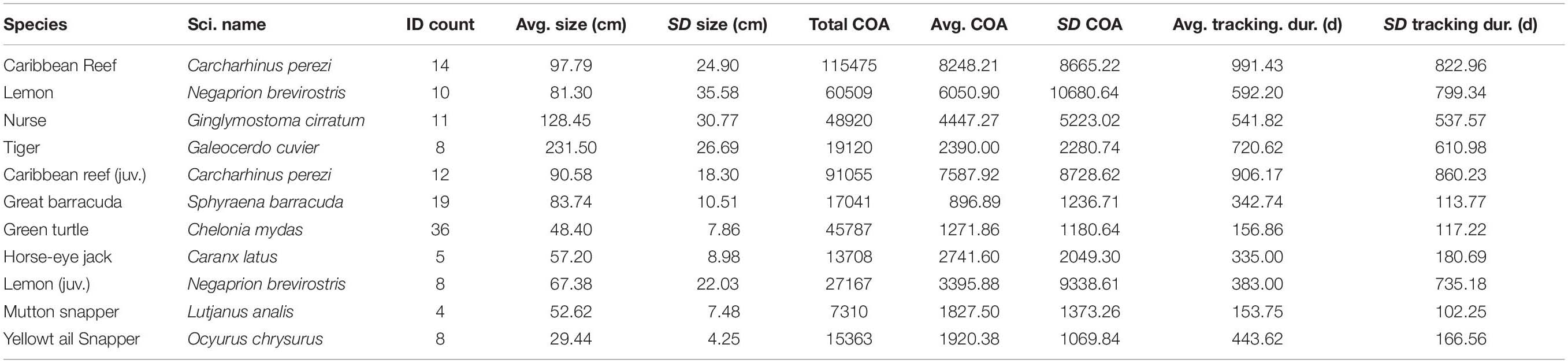
Table 1. Tagging and detection data for shark species and the potential prey species for tiger sharks, including a subset of juvenile Caribbean reef and lemon sharks, monitored within Buck Island National Monument.

TABLE 2

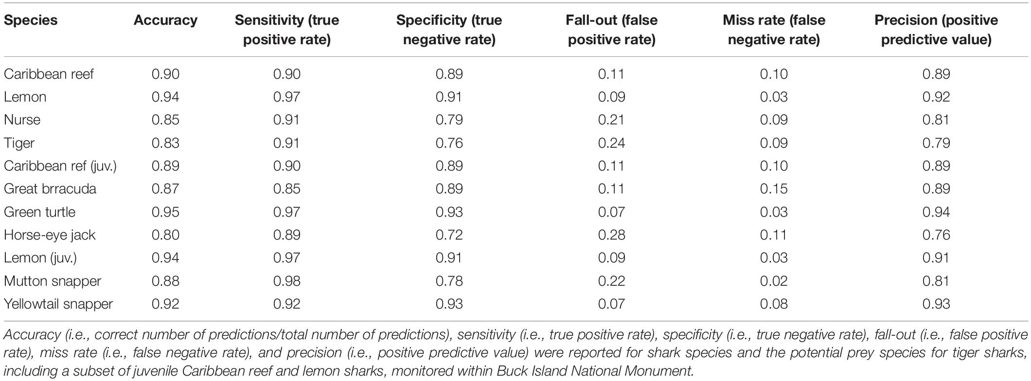
Table 2. Confusion matrix performance metrics derived from using the trained random forest model to predict across the 40% holdout dataset.

FIGURE 2

Figure 2. Feature importance, indicating how important each predictor variable is within each shark random forest model for (A) Caribbean reef sharks, (B) lemon sharks, (C) nurse sharks, and (D) tiger sharks. Higher values and darker colors indicate greater relative importance. Values were calculated using the mean decrease in accuracy method and, subsequently, all importance values were normalized from 0 to 1 for comparison across species.

FIGURE 3

Figure 3. Random forest partial dependency (marginal effects, ŷ) plots for the top three most important (ordered from top to bottom) predictors for (A) Caribbean reef sharks, (B) lemon sharks, (C) nurse sharks, and (D) tiger sharks. The marginal effects indicate the relative selection strength for the given variable with greater ŷ values indicating high relative selection probabilities and lesser values indicating low relative selection probabilities. Discrete predictors are displayed with bar plots and continuous predictors are displayed using a generalized additive model smoother with 95% confidence intervals. Partial dependency plots involving depth were restricted to 50 m depth for each species.

Caribbean reef sharks were more likely to select for coral or coral-containing habitats with higher ŷ values observed within coral habitats (sand with scattered coral and rock, aggregate reef, and aggregated patch reefs) (Figure 3A). Caribbean reef shark two-way predictor interactions highlighted relatively high ŷ values in depths of 20–30 m, areas <2 km away from land, and in areas of sand with scattered coral and rock (Figure 4A). Lemon sharks were more likely to select for shallow areas directly adjacent to land, specifically in shallow (0–5 m) habitats classified as channel, lagoon, and reef crest (Figures 3B, 4B). While nurse sharks followed a similar pattern, ŷ values indicated they were more likely to select for habitats between 0 and 2,000 m away from land but within <15 and 25–30 m of depth. In addition, ŷ values were higher in areas of sand with scattered coral and rock located within bank/shelf, bank/shelf escarpment, fore reef, and reef crest zones (Figures 3C, 4C). Lastly, tiger sharks exhibited the greatest ŷ values away from land (500–2,000 m), in <30 m depth, and in aggregate reef, sand, sand with scattered coral and rock, and pavement habitats (Figures 3D, 4D).

FIGURE 4

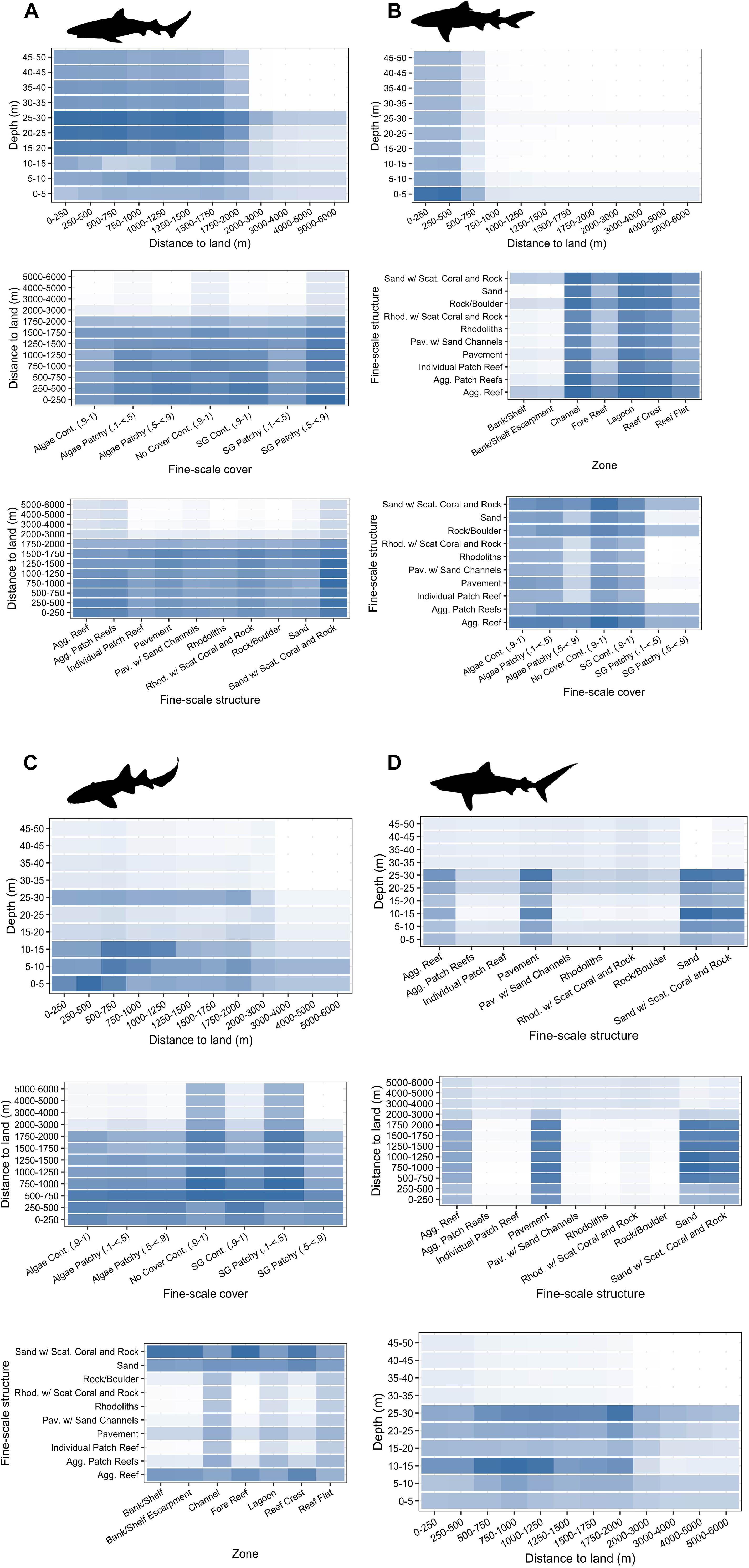
Figure 4. Top three two-way interactions (ordered from top to bottom) displayed and extracted from random forest models for (A) Caribbean reef sharks, (B) lemon sharks, (C) nurse sharks, and (D) tiger sharks. Mean marginal effects (ŷ) are shown in each two-way interaction partial dependency plot with colors indicating a continuum from high (blue) to low (white) probabilities of relative selection. Partial dependency plots involving depth were restricted to 50 m depth for each species.

Extrapolated relative habitat selection values across BIRNM, as computed from the trained RF models, followed similar patterns to kernel density estimates (Figure 5). Specifically, 50% kernel density estimates largely overlapped with extrapolated areas of high relative selection. However, for Caribbean reef, nurse, and tiger sharks, levels of high extrapolated relative selection also extended beyond 50% kernel density estimates along the western shelf and the eastern side of BIRNM, where receiver coverage was limited. While Caribbean reef, lemon, and tiger sharks exhibited more targeted habitat selection with greater affinities to specific areas and habitats, nurse sharks exhibited a more generalist approach to relative habitat selection across BIRNM (Figure 5). Caribbean reef sharks showed strong affinity to habitats with reef-containing structure, including areas of linear reef around the island and in the aggregated patch reef system that is characteristic north of the island (Figure 5A). In addition, Caribbean reef sharks exhibited higher relative selection values along the western shelf near adjacent deep water habitats (>50 m). Alternatively, lemon shark relative habitat selection values were tightly located around the island, within the reef sheltered lagoon, with lower values along the southwest side of the island where less lagoon and structure habitat exist (Figure 5B). Nurse shark extrapolated relative selection values were wide ranging with the densest cluster of higher values surrounding the island (reef habitats), to the southwest of the island along the bank (sand and seagrass habitats), and to the far eastern side of BIRNM (reef, pavement, and sand habitats) (Figure 5D). Lastly, similar to nurse sharks, tiger sharks primarily have highest selection values extrapolated south of the island along banks containing both seagrass and sand habitats, leading to the continental shelf break in the west. Relative selection values were also expected to be high along the western shelf and in some locations around the north/northwest shelf. While low relative selection values were expected for tiger sharks in the network of highly rugose patch reefs north of the island, higher selections values existed on eastern side of BIRNM habitats containing mainly reef, pavement, and sand (Figure 5D).

FIGURE 5

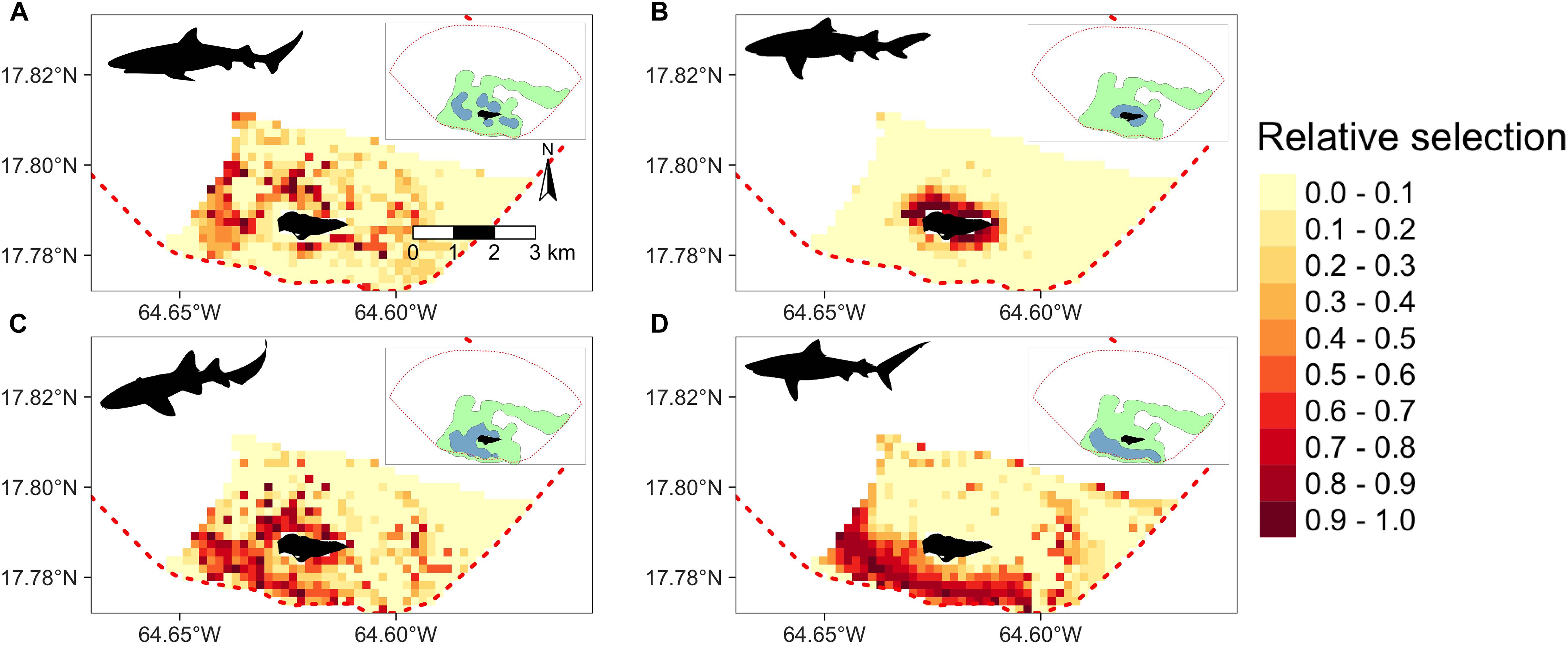
Figure 5. Derived from random forest models, the predicted and extrapolated probability of relative selection across Buck Island National Reef Monument (designated by red dashed line) for (A) Caribbean reef sharks, (B) lemon sharks, (C) nurse sharks, and (D) tiger sharks. Higher and darker values indicate higher relative selection values. Model extrapolation across the study areas restricted to the maximum observed depth for each species. 50% (green) and 95% (blue) kernel density estimates shown in the upper right corner of each plot.

Predator-Prey Relationships

Resource selection functions were also extended to examine potential areas of relative selection overlap between tiger sharks and their potential prey sources. Depending on the species, overlap selections varied in location and intensity. For example, juvenile green turtles (Figure 6A) and tiger sharks were most likely to overlap in selection south of the island where seagrass beds along bank habitats were most abundant. For juvenile Caribbean reef sharks and tiger sharks, averaged overlap selection values were greatest along the western shelf and in the southwest portion of BIRNM (Figure 6B). Juvenile Caribbean reef sharks also had high relative selection values north of the island, averaged overlap was comparatively lower in this area to the western shelf due to reduced tiger shark selection values (Figure 5D). The averaged overlap selection values between barracuda and tiger sharks followed a similar pattern with higher barracuda relative selection values north of the island but averages reduced due to lower tiger shark relative selection values (Figure 6C). Horse-eye jacks, with the most similar relative selection values of tiger sharks, had the greatest averaged overlap values along the western shelf, south of the island, and in the southeastern portion of BIRNM (Figure 6D). When tiger shark relative selection values were averaged across the other three species, including juvenile lemon sharks, mutton snapper, and yellowtail snapper, they followed similar patterns with higher averaged relative selection overlap values where the potential prey species had higher selection values unless it was directly north of the island where patch reef systems exist (Supplementary Figure 4).

FIGURE 6

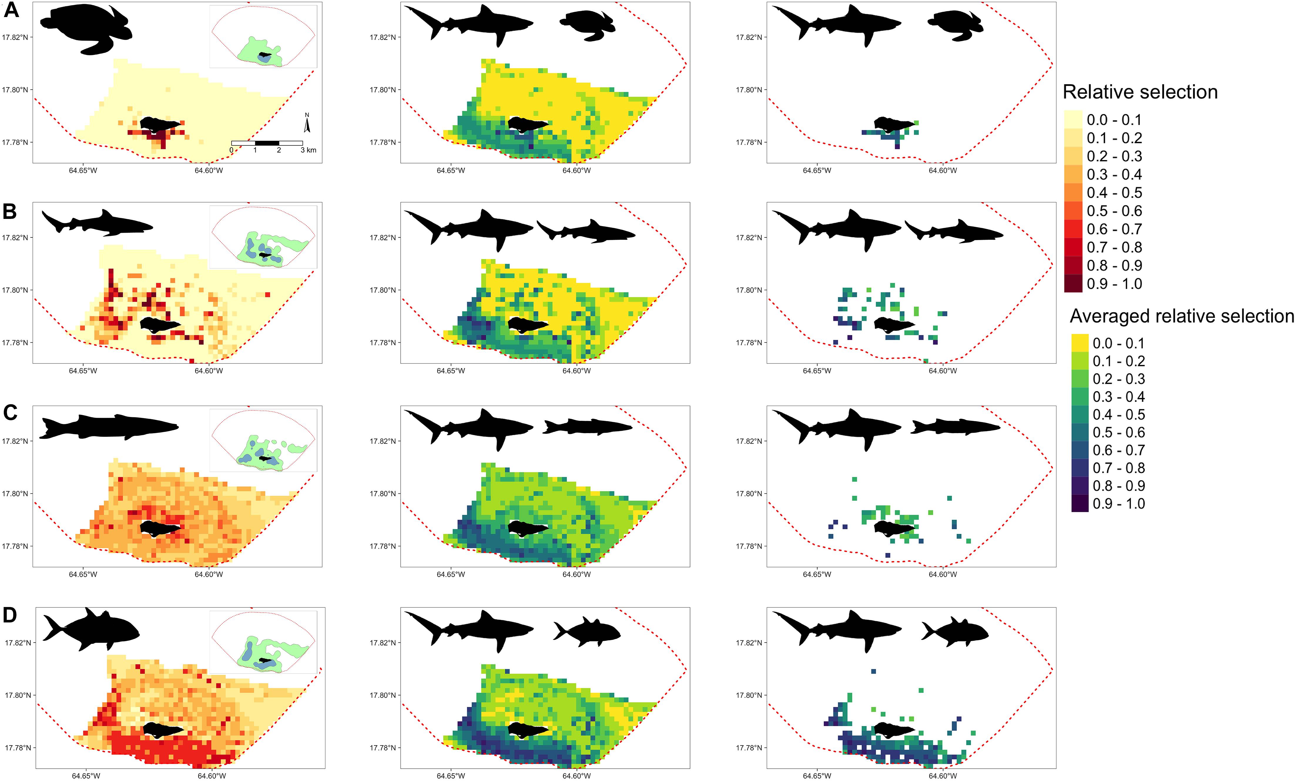
Figure 6. (Left) Derived from random forest models, the predicted and extrapolated probability of relative selection across Buck Island National Reef Monument (designated by red dashed line) for (A) juvenile green turtles (B) juvenile Caribbean reef sharks, (C) great barracuda, and (D) horse-eye jacks. 50% (green) and 95% (blue) kernel density estimates shown in the upper right corner of each plot. (Middle) Relative selection values averaged between tiger sharks and each corresponding species on the left. (Right) Relative selection values averaged between tiger sharks and each corresponding species on the left after the removal of cells where potential prey relative selection values were <.5. In all plots, higher and darker values indicate higher relative selection values or their averages.

Additional Methodological Considerations

The RF models using COA data of 60-min bins produced similar results to models that used COA data of 90-min bins (Appendix B). The top two most important variables remained unchanged for all shark species (Appendix Figure B1) and pdps and associated ŷ values only changed slightly (Appendix Figure B2). Most notably, the new 60-min binned RF models indicated ŷ values generally increased (rather than decreased) with depth for Caribbean reef sharks and ŷ values for aggregate reef were lower for tiger sharks (Appendix Figures B2, B3). However, for Caribbean reef sharks, ŷ values related to depth remained similar across the interaction of depth and distance to land.

While accuracy metrics were similar for all species across the 60- and 90-min RF models (∼1–2% differences), some varied substantially (e.g., 5–7%) (Table 2 and Appendix Table B1). The use of 60-min time bins led to a decrease in overall accuracy for nurse sharks (85–80%) but an increase in overall accuracy for barracuda (87–92%), horse-eye jack (80–90%), and mutton snapper (88–96%). Subsequently, model predictions and extrapolations within BIRNM reflected these discrepancies with lower accuracy scores producing more homogenous and generalized relative habitat selection patterns than when models produced higher predictive accuracies (Figures 5, 6 and Appendix Figures B4, B5).

RF models using 200 m buffers for available habitat construction scored lower accuracy measurements and also predicted higher relative selection homogeneously across BIRNM (Supplementary Figure 5 and Supplementary Table 1). Alternatively, models using 600 m buffers for available habitat construction produced similar accuracy measures and predictions across BIRNM as compared to the original models (Supplementary Figure 5 and Supplementary Table 1). Interestingly, relative selection predictions for tiger sharks were higher along the northeastern shelf edge (Supplementary Figure 5) than in the original model (Figure 5), matching Casselberry et al. (2020) findings.

When assessing extrapolation reliability across BIRNM, extrapolation space became unreliable (univariate extrapolation) in areas off the shelf in deeper and further areas from land (Appendix A). However, areas within the MPA that remained in shallower water (<50 m) were analogous to the range of our covariates as measured by depth (m) and distance to land (m), confirming our approach to limiting extrapolations to the maximum observed depth was warranted.

While BBMMs highlighted individual level variation in space use across BIRNM (see examples, Supplementary Figure 6), GLMMs and respective marginal and conditional R² values indicated variance was largely explained by the fixed effects (marginal R²) alone (Supplementary Table 2). However, the GLMM involving lemon sharks appeared to have substantial variance explained by both the fixed and random effects combined (conditional R²), suggesting individual variation may be higher within this species dataset. Interestingly, GLMM accuracy for lemon sharks was also nearly as accurate as the RF model (92% versus 94%, respectively). Accuracy metrics for the other GLMMs were substantially lower than respective RF models (Table 2 and Supplementary Table 2).

Discussion

The Approach and Ecological Implications

Using acoustic telemetry data for four shark species, we demonstrate the utility of RSFs with machine learning to accurately predict and understand complex environmental drivers of marine species. Across species, we found variable patterns of relative habitat selection within the MPA, ranging from habitat specialists to generalists. Overall, as depth increased, relative selection decreased for all shark species. While relative selection probabilities for Caribbean reef, lemon, and nurse sharks decreased as distances from land increased, tiger sharks showed highest affinities for areas between 500 and 2,000 m away from land. Top interactions along with predicted relative selection values highlighted the differences and preferences across species in terms of habitat types, structures, and depths. Finally, using the relative selection values of tiger sharks and their potential prey, we highlight the ability of this framework to generate multiple species selection values that could provide insights into predator-prey relationships when averaged and overlaid with one another.

The results for shark habitat selection presented herein are largely consistent with those presented by Casselberry et al. (2020) that used GLMMs and detection data from fixed receiver locations to model presence in BIRNM habitats, but with improved model accuracy (83–94%) and additional covariates. While GLMMs in Casselberry et al. (2020) were limited by unequal receiver distribution, requiring aggregation across habitat types, the analyses presented here (use/availability framework with COAs and background points) were able to sample across multiple habitats and at finer scales. Further, while GLMMs were limited to a single generalized habitat covariate (factor levels including: unconsolidated sediments, submerged vegetation, and coral, rock, and colonized hardbottom) and depth, RSFs paired with machine learning algorithms were able to easily assess five separate habitat covariates that ranged from two and 10 factor levels each along with two additional continuous predictors. Ultimately, RSFs confirmed use of shallow water habitats near land for lemon sharks and the use of sand and coral associated habitats at mid-depths for nurse sharks, while highlighting tiger sharks’ affinity for the continental shelf break and southern sand and seagrass beds. The added analytical flexibility of RSFs and machine learning greatly improved predictions of habitat use for Caribbean reef sharks, whose space use changes dramatically with age across BIRNM’s varied landscape (Casselberry et al., 2020). Previous models showed low probability of presence in the acoustic array across habitats and depths compared to the other three shark species, while RSFs highlight specialized use of multiple highly rugose reef habitats at mid-depths. However, GLMMs produced in Casselberry et al. (2020) and the RSF models produced here differed when predicting tiger shark depth preference. Casselberry et al. (2020) showed probability of presence in the acoustic array increasing with depth across habitat types (coral, rock, and colonized hardbottom, submerged vegetation, and unconsolidated sediments), while ŷ values consistently decreased with depths beyond 30 m in RSF models.

Examining the tiger shark partial dependency plots reveals high interactions between depth and distance to land at depths between 10–15 and 25–30 m (Figure 4). These same depth bins (10–15 and 25–30 m) also had higher ŷ values when combined with aggregate reef, pavement, sand, and sand with scattered coral and rock habitats (Figure 4). These habitat types and distance to land achieved higher ŷ values alone than depth in tiger shark models indicating that these variables have a stronger influence on tiger shark habitat use (Figure 3). However, tiger sharks are known to use depths greater than 50 m in and around BIRNM that are beyond the depths of acoustic array coverage (Casselberry unpublished data). This, again, highlighted the need to assess extrapolation reliability (Mesgaran et al., 2014) of RSFs prior to model interpretation since they may have limited ability to extrapolate outside of observed conditions of a given array, for example in areas of BIRNM where depths were greater than 50 m.

When predictions were made within our range of covariates in analogous conditional space (less than 50 m depth), the application of RSFs, as opposed to more traditional use of COAs alone, kernel density estimates, or network analyses, highlighted potentially favorable habitats in BIRNM with limited receiver coverage. The eastern portion of BIRNM has had limited acoustic receiver coverage in part because of the complexity of the coral reef structure in the area. Receiver moorings were not established there in order to avoid damaging the protected reef structure. The RSFs show that favorable habitats exist in this low coverage region for nurse, Caribbean reef, and tiger sharks, particularly at intersections between reef, pavement, and sand habitats. This further highlights the suitability of this MPA for shark conservation and management in St. Croix (Figure 5; Casselberry et al., 2020).

Examining overlapping RSFs between tiger sharks and their potential prey highlights regions of potential foraging success for sharks, high predation vulnerability for prey, and areas of ecological importance for managers. Areas of high tiger shark-prey overlap coincide mainly with the seagrass beds south of Buck Island and the western continental shelf break, while many potential prey species also have high selection potential in areas north of Buck Island. This could be a reflection of tiger sharks selectively using areas with higher potential for foraging success (Heithaus et al., 2002). Areas north of the Buck Island are occupied by highly complex coral reef habitats, offering ample areas to refuge or escape from predators (Hixon and Beets, 1993), while habitats south and west of Buck Island are more open at depths of ∼12 m. These waters could be more maneuverable for large juvenile and adult tiger sharks when compared to more structurally complex environments (Fu et al., 2016), perhaps with an increased possibility of foraging success (Heithaus and Dill, 2002; Heithaus et al., 2007; Wirsing et al., 2007). Alternatively, these areas could be a reflection of similar habitat preferences and ecologies among apex and mesopredators in a tropical reef system (Ledee et al., 2016; Heupel et al., 2019). Regardless, areas of high averaged relative selection highlight important regions in BRINM that could be used to inform future habitat monitoring or restoration studies, particularly with the potential for habitat degradation as the climate changes (Graham et al., 2020; Hastings et al., 2020).

As technological tools continue to advance our ability to monitor aquatic animal space use, ecologists are beginning to answer some of the most pressing questions to help direct and prioritize resource management and conservation strategies. Habitat destruction remains on the forefront of decreases in biodiversity, from climate change (Pratchett et al., 2011; Descombes et al., 2015) to destructive landscape use (Rothschild et al., 1994; Coverdale et al., 2013). With calls to protect at least 30% of the ocean by 2030 through establishing MPAs (O’Leary et al., 2016; Sala et al., 2018), an accurate understanding of how marine animals use space and select habitats is increasingly imperative for well informed and effective marine spatial planning (Foley et al., 2010; Ogburn et al., 2017; Lowerre-Barbieri et al., 2019; Gallagher et al., 2021; Roberts et al., 2021). The RSF modeling framework provided here can produce high accuracy models of relative habitat selection for multiple species of differing ecologies and can be averaged across species to highlight overlapping potential space use or selection. These models can then be used to extrapolate to areas lacking acoustic receiver coverage, as long as within the original measured parameters, accounting for a common issue in acoustic telemetry with incomplete coverage of the study site due to logistic or budgetary limitations. Assuming a sufficient number of individuals are tagged for a given species and age class, the outputs of these models can produce easily interpretable maps for highlighting regions of importance and communicating results to stakeholders, which could result in greater acceptance of study findings given committed stakeholder engagement (Nguyen et al., 2019).

Benefits, Challenges, and Considerations

As technological advancements (e.g., from remote sensing to acoustic telemetry data) allow for high-resolution datasets, machine learning approaches have become increasingly adopted by ecologists because of their ability to handle large datasets and complex non-linear hierarchical relationships and statistical assumptions that are typically violated by conventional parametric approaches, e.g., multiple correlated predictors (Olden et al., 2008; Peters et al., 2014; Durden et al., 2017; Brownscombe et al., 2020). While RSFs have typically been applied within a classical statistical framework (e.g., logistic and linear models) (Johnson et al., 2006; Manly et al., 2007), machine learning does not require non-linear predictor relationships and their interactions to be specified prior to implementing. Thus, allowing for a flexible, realistic, and accessible application when applying RSFs to animal space use in relation to multiple and complex environmental gradients across a landscape (Shoemaker et al., 2018). Further, implementing machine learning with ecological data can also provide highly accurate predictive models (Cutler et al., 2007; Elith et al., 2008; Olden et al., 2008). For instance, Shoemaker et al. (2018) applying RSFs with mule deer (Odocoileus hemionus) telemetry data demonstrated machine learning algorithms outperformed the traditional approach of logistic regression with higher prediction accuracy. In another example, although not directly comparable, when implementing a RF using the juvenile green turtle data in this study, we found a higher accuracy compared to that as reported by Griffin et al. (2020) (0.95 versus 0.77, respectively), who also applied RSFs on juvenile green turtle acoustic telemetry data from BIRNM but were fitted with GLMMs and fewer predictor variables.

While machine learning algorithms offer some advantages as an accurate non-parametric technique, the difficulty to account for spatial-temporal autocorrelation and individual level effects presents additional challenges. Whereas RF models are unable to easily incorporate, RSF GLMMs can explicitly include individual ID as a random effect (Gillies et al., 2006). Further, generalized models can incorporate autocorrelation dependency structures (Zuur et al., 2017; Winton et al., 2018a; Griffin et al., 2019; Gutowsky et al., 2020), however, it is worth noting that defining the correct correlation structure still remains challenging within a use/availability (presences/pseudo-absences) sampling design (see Koper and Manseau, 2009; Fieberg et al., 2010). In this study, while BBMMs highlighted individual variation in space use, simplified GLMMs indicated including individual as a random effect contributed relatively less to explaining overall variance than the fixed effects alone. However, this was not the case for lemon sharks, suggesting larger potential differences in relative habitat selection across individuals. Confirmed by individual BBMMs and network analyses from Casselberry et al. (2020), some lemon sharks were consistently close to the island while others used areas farther away and at greater depths. While approaches are being developed to incorporate mixed effects into machine learning algorithms (Hajjem et al., 2014), it is still relatively inaccessible due to its complexity. Future studies using RSFs and machine learning algorithms should attempt to measure or address random variation across individuals and sample size biases either within the approach and/or with complimentary analyses. For example, using test datasets that contain individuals not used in the training dataset may better help to assess model performance and transferability (Buston and Elith, 2011; Raymond et al., 2015). Further, running models for each individual and, subsequently, collectively deriving the 95% confidence interval estimates across the computed marginal effects for all individuals may be a viable approach to assess population level effects. Alternatively, using both mixed effects models and machine learning approaches in tandem may be the most appropriate (see Shoemaker et al., 2018). With consideration to this caveat, machine learning algorithms provide useful and flexible advantages to deal with complex ecological datasets and to obtain accurate results.

Beyond the application of RSFs with machine learning algorithms, by design, passive acoustic telemetry arrays provide an intuitive approach for implementing RSFs since available resource units can easily be defined based upon receiver positioning. Constraining COAs and background points to the available resource units, defined by acoustic receiver location at the year level, allows for the incorporation or removal of additional receivers across a study period. This flexibility is ideal as arrays often change over time due to funding constraints or adapting research questions. However, to safeguard against biased relative selection estimates, it is important to ensure receiver arrays, including their modifications, are designed to capture space use that is representative of the habitat available (Selby et al., 2019; Griffin et al., 2020). For future studies aimed at examining relative selection, we suggest grid array designs (Heupel et al., 2006; Kraus et al., 2018) to achieve proportionally representative coverage of areas rather than deployments guided by a priori beliefs of animal space use (Brownscombe et al., 2019b). In addition, detection range and efficiency, should be considered during the array design (Brownscombe et al., 2019b), when constructing COAs (Winton et al., 2018b), when defining available resource units around receivers, or even explicitly in the modeling process (see Brownscombe et al., 2019a). Detection efficiency and range, often limited by physical structure, wind, currents, animal noise, or by human activities may vary greatly across a given study area (Gjelland and Hedger, 2013; Kessel et al., 2014).

Here, while potentially incorporating biases due to variable detection ranges (see Selby et al., 2016), we chose a 400 m buffer around each receiver to allow for COAs and associated background points to extend beyond observed detection ranges. However, we recommend testing a wide range of parameter inputs from COA time bin selection to available habitat buffer size. Such inputs should be guided by ecological knowledge, acoustic telemetry coverage, and model accuracy metrics. While COA time bins of 60-min provided more accurate measures for some species and refined predictions, we opted for 90-min bins for all species since this would potentially reduce issues with autocorrelation by subsampling further (Swihart and Slade, 1985). Further, COA time bin selection should consider both the programmed tag delay and the speed of tagged animals, with smaller time bins for faster moving species and larger time bins for slow moving animals. In this example, we found a smaller available habitat buffer produced lower accuracy metrics and led to unreliable predictions across BIRNM. Alternatively, applying a larger available habitat buffer provided similar results to the original models that used 400 m buffers and also captured relative selection for tiger sharks in areas (northeast shelf) where we expected higher values. While 400 m buffers were chosen for consistency to Selby et al. (2019) and Griffin et al. (2020), future researchers should explore and evaluate multiple extents for a given species, study area, and array. Along with variable detection range and efficiency, future RSF studies using acoustic telemetry should also investigate the role of spatial and/or temporal scales on selection modeling (McGarigal et al., 2016); this is especially relevant when collapsing habitat and presences/background points for model implementation.

Conclusion

In summary, we highlight the utility of combining acoustic telemetry, RSFs, and machine learning to understand and accurately predict the relative habitat selection of marine animals across both monitored and unmonitored areas. While RSFs have been used extensively within terrestrial environments, we suggest marine ecologists should also adopt these methods to improve resource management actions. Such applications could help to prioritize habitat protection and restoration in the face of continued anthropogenic threats (Millennium Ecosystem Assessment, 2003). This may have particular advantages centered around MPA design. Here, applied to four shark species within an MPA, we found accurate models that could extrapolate to areas where receiver coverage was limited. Further, when these RSF values were extended to examine predator-prey relationships, we found areas that varied in mutual selection, highlighting the potential overlap of predators and their prey.

Data Availability Statement

The datasets generated for this study are not readily available because studies for each individual species are currently ongoing. Data can be made available upon reasonable request through GC at grace.casselberry@gmail.com or directly to the data owners: GS (sharks), AJ (reef fish), and KH (sea turtles). Code for the resource selection function framework with a sample dataset can be found at https://github.com/lucaspgriffin.

Ethics Statement

The animal study was reviewed and approved by University of Massachusetts Amherst IACUC no. 2013-0031 and 2019-0043. Research conducted within BIRNM was approved by NPS under study no. BUIS-00058 and individual research collection permit nos. BUIS-2013-SCI_0003, BUIS-2014-SCI-0006, and BUIS-2019-0010. For green turtle fieldwork, permitting was under NMFS permits 16146 and 20315, issued to KH, National Park IACUC USGS-SESC2014-02 and USGS IACUC WARC\GNV 2017-04. Additional permits issued to KH BUIS-2011-SCI-0012; BUIS-2014-SCI-0009; BUIS-2016-SCI-0009. Acoustic receiver stations were deployed under the following permit numbers through the United States Army Corp of Engineers: SAJ-2014-01790, SAJ-2015-02061, SAJ-2015-02062, SAJ-2017-00622, and SAJ-2017-00624.

Author Contributions

LG and GC conceived and led the study. GC, KH, AJ, SB, AN, BD, CP, IL, ZH-S, AD, and GS conducted the field work. LG analyzed the data. All authors interpreted the findings, wrote the manuscript, and approved the final version.

Funding

This work was supported by grants from the following funders: Puerto Rico Sea Grant (R-101-2-14), The New England Aquarium’s Marine Conservation Action Fund, The Atlantic White Shark Conservancy, National Geographic Society, The Allen Family Foundation, and the USGS Natural Resource Protection Program and USGS Ecosystems Program.

Conflict of Interest

The authors declare that the research was conducted in the absence of any commercial or financial relationships that could be construed as a potential conflict of interest.

Acknowledgments

We acknowledge the USGS Natural Resource Protection Program (NRPP) for funding. AD was supported by the National Institute of Food and Agriculture, United States Department of Agriculture, the Massachusetts Agricultural Experiment Station, and the Department of Environmental Conservation. GC was supported by the NOAA ONMS Dr. Nancy Foster Scholarship. We thank the numerous National Park Service staff and interns for their work maintaining BIRNM receiver array throughout the years, especially Tessa Code and Nathaniel Hanna Holloway. We also thank Jake Brownscombe and Laura D’Acunto for review of an earlier draft of the manuscript. We thank Brace Thompson for providing his artistic talents to figure one. Finally, we thank the reviewers and associate editor for thorough and constructive feedback. Any use of trade, product, or firm names is for descriptive purposes only and does not imply endorsement by the United States Government.

Supplementary Material

The Supplementary Material for this article can be found online at: https://www.frontiersin.org/articles/10.3389/fmars.2021.631262/full#supplementary-material

Abbreviations

BIRNM, Buck Island Reef National Monument; BBMM, Brownian bridge movement model; COAs, centers of activity; GLMM, generalized linear mixed model; MPA, marine protected area; RF, random forest; RSF, resource selection function.

References

Aarts, G., MacKenzie, M., McConnell, B., Fedak, M., and Matthiopoulos, J. (2008). Estimating space−use and habitat preference from wildlife telemetry data. Ecography 31, 140–160. doi: 10.1111/j.2007.0906-7590.05236.x