Element-Selective Targeting of Nutrient Metabolites in Environmental Samples by Inductively Coupled Plasma Mass Spectrometry and Electrospray Ionization Mass Spectrometry

Metabolites that incorporate elements other than carbon, nitrogen, hydrogen and oxygen can be selectively detected by inductively coupled mass spectrometry (ICPMS). When used in parallel with chromatographic separations and conventional electrospray ionization mass spectrometry (ESIMS), ICPMS allows the analyst to quickly find, characterize and identify target metabolites that carry nutrient elements (P, S, trace metals; “nutrient metabolites”), which are of particular interest to investigations of microbial biogeochemical cycles. This approach has been applied to the study of siderophores and other trace metal organic ligands in the ocean. The original method used mass search algorithms that relied on the ratio of stable isotopologues of iron, copper and nickel to assign mass spectra collected by ESIMS to metabolites carrying these elements detected by ICPMS. However, while isotopologue-based mass assignment algorithms were highly successful in characterizing metabolites that incorporate some trace metals, they do not realize the whole potential of the ICPMS/ESIMS approach as they cannot be used to assign the molecular ions of metabolites with monoisotopic elements or elements for which the ratio of stable isotopes is not known. Here we report a revised ICPMS/ESIMS method that incorporates a number of changes to the configuration of instrument hardware that improves sensitivity of the method by a factor of 4–5, and allows for more accurate quantitation of metabolites. We also describe a new suite of mass search algorithms that can find and characterize metabolites that carry monoisotopic elements. We used the new method to identify siderophores in a laboratory culture of Vibrio cyclitrophicus and a seawater sample collected in the North Pacific Ocean, and to assign molecular ions to monoisotopic cobalt and iodine nutrient metabolites in extracts of a laboratory culture of the marine cyanobacterium Prochorococcus MIT9215.

Introduction

Advances in the chromatographic separation and mass spectral analyses of metabolites have opened new avenues for understanding microbial dynamics and organic matter cycling in the ocean (Petras et al., 2017; Patriarca et al., 2018). Marine environmental metabolomics, the comparative analysis of metabolites expressed in particulate or dissolved organic matter sampled under different conditions, is typically approached in one of two ways: through targeted metabolomics in which metabolites of interest are measured through an experiment or suite of samples, and untargeted metabolomics in which the response of unidentified metabolites are correlated against experimental or environmental variables (reviewed by Soule et al., 2015; Cajka and Fiehn, 2016). Each approach comes with trade-offs between the confidence in metabolite identity or amount with the breath of metabolites that are measured. The targeted approach allows for high confidence in metabolite identity and concentration, but is limited to select and spectrally characterized compounds. Untargeted approaches survey a much broader suite of metabolites, but in doing so a detailed knowledge of metabolite identity and quantity is sacrificed. These two approaches bookend other avenues for investigating marine metabolomics that share features with both targeted and untargeted analyses. Here we discuss an approach that combines multi-modal liquid chromatography mass spectrometry data sets to target metabolites containing specific elements. However, the approach can easily be adapted and applied to metabolites that share other chemical properties such as UV/Vis light absorption or fluorescence.

Nutrient availability drives many microbial biogeochemical cycles, and investigations of how nutrient dynamics impact marine genomes, proteomes, and metabolomes are becoming increasingly common. Methods that target metabolites carrying nutrient elements such as nitrogen, phosphorus, sulfur and bioactive trace metals (Fe, Cu, Zn, Ni, Mn, Co), are therefore of interest. Metabolites incorporating nutrient elements (nutrient metabolites) can be separated in extracts of microbial biomass, dissolved and particulate organic matter by liquid chromatography (LC) and selectively detected by inductively coupled plasma mass spectrometry (ICPMS), enabling a nutrient or element-targeted approach to marine metabolomics. ICPMS is highly sensitive, with femtomole detection limits. However, other than the presence and amount of the nutrient element, LC-ICPMS only characterizes metabolites by their chromatographic retention time. This shortcoming can be addressed by combining LC-ICPMS data with companion mass spectral data obtained from high-resolution electrospray ionization mass spectrometry (LC-ESIMS). LC-ESIMS can be used to identify metabolites, or for unknown compounds, determine their molecular weight, elemental composition, and major ions after MS/MS fragmentation. As an application of this element-targeted metabolomics approach, we have used LC-ICPMS and LC-ESIMS to characterize trace metal organic complexes in laboratory cultures of marine cyanobacteria (Boiteau and Repeta, 2015) and marine dissolved organic matter (Boiteau et al., 2016, 2019; Bundy et al., 2018).

In seawater, most bioactive trace metals (Fe, Cu, Zn, Co, Ni, etc.) are complexed to dissolved organic ligands (>99.9% of Fe, reviewed in Gledhill and Buck, 2012; > 98% of Cu, Buckley and van den Berg, 1986; Coale and Bruland, 1988, 1990; > 98% of Zn, Bruland, 1989; > 99% of Co, Saito and Moffett, 2001; 10–20% of Ni, Achterberg and Van Den Berg, 1997). Organic ligands elevate the solubility of trace metals (Kuma et al., 1998; Millero, 1998), but also play a crucial role in their bioavailability (Hutchins et al., 1999; Wells and Trick, 2004; Hassler et al., 2011; Aristilde et al., 2012; Lis et al., 2015). Some trace metal organic complexes are readily available to microbes, while others are not. For example, microbial production in approximately one third of the surface ocean is limited by the bioavailability of iron (Boyd et al., 2007; Moore et al., 2013). Microbes inhabiting these iron-limited regions produce siderophores, organic compounds synthesized to bind iron and facilitate iron uptake (Reid et al., 1993; Martinez et al., 2000, 2001). Microbes expressing appropriate cross-membrane siderophore transport systems are able to take up siderophore-bound iron to help satisfy their iron requirements (Hopkinson and Barbeau, 2012; Tang et al., 2012). Cataloging where siderophores are made in the ocean, and under what conditions, contributes to our understanding of how marine microbes respond to iron bioavailability. However, hundreds of different siderophores, most likely representing only a fraction of the siderophores produced in nature, have been identified in laboratory cultures (Hider and Kong, 2010; Baars et al., 2014). Compounding this, marine dissolved organic matter is an extraordinarily complex mixture of 10⁵ to 10⁶ different compounds. Ideally, methods for analyzing siderophores or other nutrient metabolites should therefore allow the analyst to quickly find and identify known siderophores or characterize new siderophores, at low concentrations and within the very complex mixture of organic compounds that is typical of most environmental samples.

Boiteau et al. (2013, 2016) described a method whereby siderophores and other nutrient element metabolites were concentrated from seawater or spent culture media by solid phase extraction (SPE), then separated by LC and detected by ICPMS. An example of the results from an analysis of siderophores in a seawater sample collected in the North Pacific Ocean is provided in Figure 1A. Siderophores appear in the iron chromatogram as a series of well-defined peaks at different retention times, which can be quantified after appropriate calibration with iron standards. The sample was then analyzed a second time using the same chromatographic conditions, but with detection by high resolution ESIMS (Figure 1B). The LC-ICPMS data and LC-ESIMS data were then integrated using mass alignment and filtering algorithms to identify the major peaks in the sample as a suite of marinobactins, amphiphilic siderophores synthesized by heterotrophic bacteria.

FIGURE 1

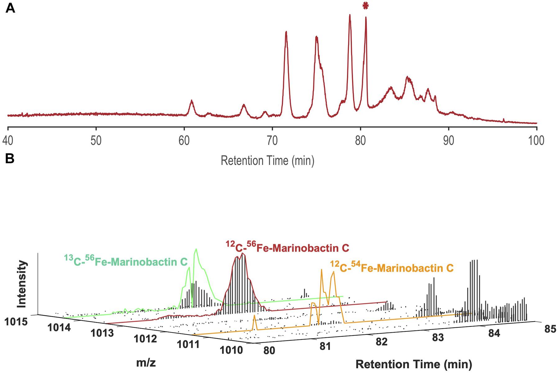
Figure 1. (A) LC-ICPMS ⁵⁶Fe-chromatogram of dissolved organic matter collected by SPE from the North Pacific Ocean. Each discrete peak represents one (or a combination of multiple) Fe-containing organic compounds. The starred peak (*) at 80.6 min was selected as our target for characterization, and (B) LC-ESIMS data between 80–85 min and 1010.00 D-1015.00 D for the same sample. Using the isotope ratio search algorithm with Δm = 1.995 D and R = 15.7 for ⁵⁴Fe and ⁵⁶Fe the peak at 80.6 min was assigned the m/z of 1013.44 D. It is then identified as marinobactin C (EIC outlined in red), by comparison of its exact m/z with a catalog of know siderophores. The scaled plots for ⁵⁴Fe-1011.45 D, and ¹³C-⁵⁶Fe-1014.44 D of marinobactin C are outlined in orange and green respectively. Each vertical black bar represents the ion intensity at each mass in a scan at a given retention time.

We have used LC-ICPMS/ESIMS method to identify and quantify pM concentrations of iron, copper, and nickel ligands in a variety of seawater and laboratory culture samples. However, the coupling of a reverse-phase LC method designed to separate relatively nonpolar mixtures of organic compounds, to ICPMS presented several analytical challenges that were not fully resolved in our original method. First, the ICPMS plasma is sensitive to solvent composition and contamination, which change through the analysis. As the concentration of methanol or acetonitrile increases in the mobile phase, the spectrometer response to iron (for example) decreased by a factor of 2–3, complicating quantitative analysis (Boiteau et al., 2013). Second, the LC eluent delivered to the ICPMS interface led to cooling or quenching of the plasma. Therefore, the method incorporated a post column split which directed a majority of a sample to waste. Finally, the mass search algorithms that combined ICPMS and ESIMS data relied on the exact mass difference (Δm) and crustal relative abundance ratio (R) of an element’s major isotopologues (Δm = 1.995 D and R = 15.7 for ⁵⁴Fe and ⁵⁶Fe, for example). For elements with low abundance isotopologues, the detection and resolution of minor isotopic forms of metabolites that occur at very low concentrations was often difficult to achieve (Figure 1B). Further, many elements of interest (Mn, Co, P, I) do not have stable isotopes pairs, and algorithms that rely on isotopic fine structure analysis are not able to assign masses to a many nutrient metabolites of interest.

Over the past few years we have made a number of improvements to the original method to increase sensitivity and accuracy, and to expand its scope to include monoisotopic elements. The entire sample is now introduced into the mass spectrometer improving sensitivity by four to fivefold. Solvent effects on detector sensitivity have been mitigated and quantified. New mass search algorithms have been coded that allow the molecular ions of metabolites incorporating monoisotopic elements, or isotope pairs for which the isotopic ratio is not known, to be assigned. Here we describe the details of the method, and provide some examples of its application to environmental metabolomics.

Materials and Methods

Reagents and Standards

High purity solvents and reagents were used throughout, including ultrapure water (18.2 MΩ; qH₂O), LCMS grade methanol (MeOH, Optima, Fisher Scientific) redistilled in a Polytetrafluoroethylene still, and LCMS grade ammonium formate (Optima, Fisher Scientific).

For reference standards, desferrichrome (as metal-free (apo) form), ferrioxamine-E and cyanocobalamin (vitamin B12) were purchased from Sigma Aldrich. Amphibactin siderophores were produced by culturing the marine bacterium, Vibrio cyclitrophicus strain 1F-53. The media consisted of 10 g casamino acids, 1 g NH₄Cl, 1.03 g Na₂HPO₄, 3 mL glycerol, and 5 mL vitamin stock solution in 1 L of 0.2 μm filtered Sargasso Sea seawater. The vitamin stock solution consisted of 40 mg biotin, 4 mg niacin, 2 mg thiamin, 4 mg 4-aminobenzoic acid, 2 mg calcium pantothenic acid, 20 mg pyridoxine HCl, 4 mg riboflavin, 4 mg folic acid, and 2 mg cyanocobalamin in 50 mL qH₂O. All vitamins are purchased from Sigma-Aldrich. We induced Fe limitation by adding 10 nM desferrioxmaine B (as desferrioxamine mesylate salt, Sigma Aldrich). The media was sterilized by 0.2 μm filtration (Fisher Scientific), then transferred into an autoclaved glass flask using axenic protocols. An incoulum of V. cyclitrophicus 1F-53 was added, the culture flask wrapped with aluminum foil and shaken at 150 rpm at room temperature until the culture became turbid and foamy (30–40 h). The culture was filtered through 0.2-μm Pall Acropak Supor cartridges, and extracted as discussed below. Equimolar amounts of ferric chloride (FeCl₃^∗6H₂O, Fisher Scientific) were added to apo ferrichrome or amphibactins to synthesize ⁵⁶Fe-siderophore complexes.

Sample Collection and Extraction

Seawater samples were collected from the North Pacific Ocean during the US GEOTRACES Pacific Meridional Transect (GP15, October 2018) expedition, using a trace metal clean GTC rosette/Go-Flo bottle sampler. Each sample was filtered directly from the Go-Flo bottle through a 0.2 μm Pall Acropak-200 Supor cartridge (Cutter et al., 2018) into an acid-cleaned polycarbonate bottle. Trace metal organic complexes were extracted from 4 L of filtered seawater pumped at 20 mL/min through Bond-Elut ENV cartridges (1 g, 6 mL, Agilent Technologies) that had been activated with ∼6 mL each of distilled MeOH, pH 2 (Optima HCl, Fisher Scientific) qH₂O, and qH₂O. SPE columns were frozen (−20^oC) immediately after sample collection and returned to the laboratory for processing. To recover samples from the ENV cartridge, columns were thawed, washed with 6 mL qH₂O, and eluted with 6 mL distilled MeOH into acid-cleaned 10 mL falcon tubes. The eluent was concentrated to 500 μL by vacuum centrifugation (SpeedVac, Thermo Scientific).

High Pressure Liquid Chromatography-Mass Spectrometry

Chromatographic analyses were performed on a bioinert Dionex Ultimate 3000 LC system fitted with a loading pump, a nano pump, and a 10-port switching valve, the schematic of which is shown in Figure 2. During the loading phase, 200 μL of sample were withdrawn into the sample loop, then pushed onto a C18 trap column (3.5 μm, 0.5 mm × 35 mm, Agilent PN 5064-8260) by the loading pump at 25 μL/min for 8 min (95% qH₂O, 5% MeOH, 5 mM ammonium formate). Solvent delivery was then switched to the nanopump, the flow rate reduced to 10 μL/min, and the trap column outflow directed onto two C18 columns (3.5 μm, 0.5 mm × 150 mm, Agilent PN 5064-8262) connected in series. Samples were separated with an 80 min gradient from 95% solvent A (5 mM aqueous ammonium formate) and 5% solvent B (5 mM methanolic ammonium formate) to 95% solvent B, followed by isocratic elution at 95% solvent B for 10 min. Meanwhile, the loading pump solvent was switched to 100% qH₂O, increased to 35 μL/min and directed as a make-up flow (qH₂O), which was infused with the column eluant (10 μL/min) into the ICPMS. Although ICPMS and ESIMS data can be collected in parallel by splitting the outflow of the LC system between the two spectrometers, in practice we found it easier to perform two separate analyses of a sample and align the data using an internal standard.

FIGURE 2

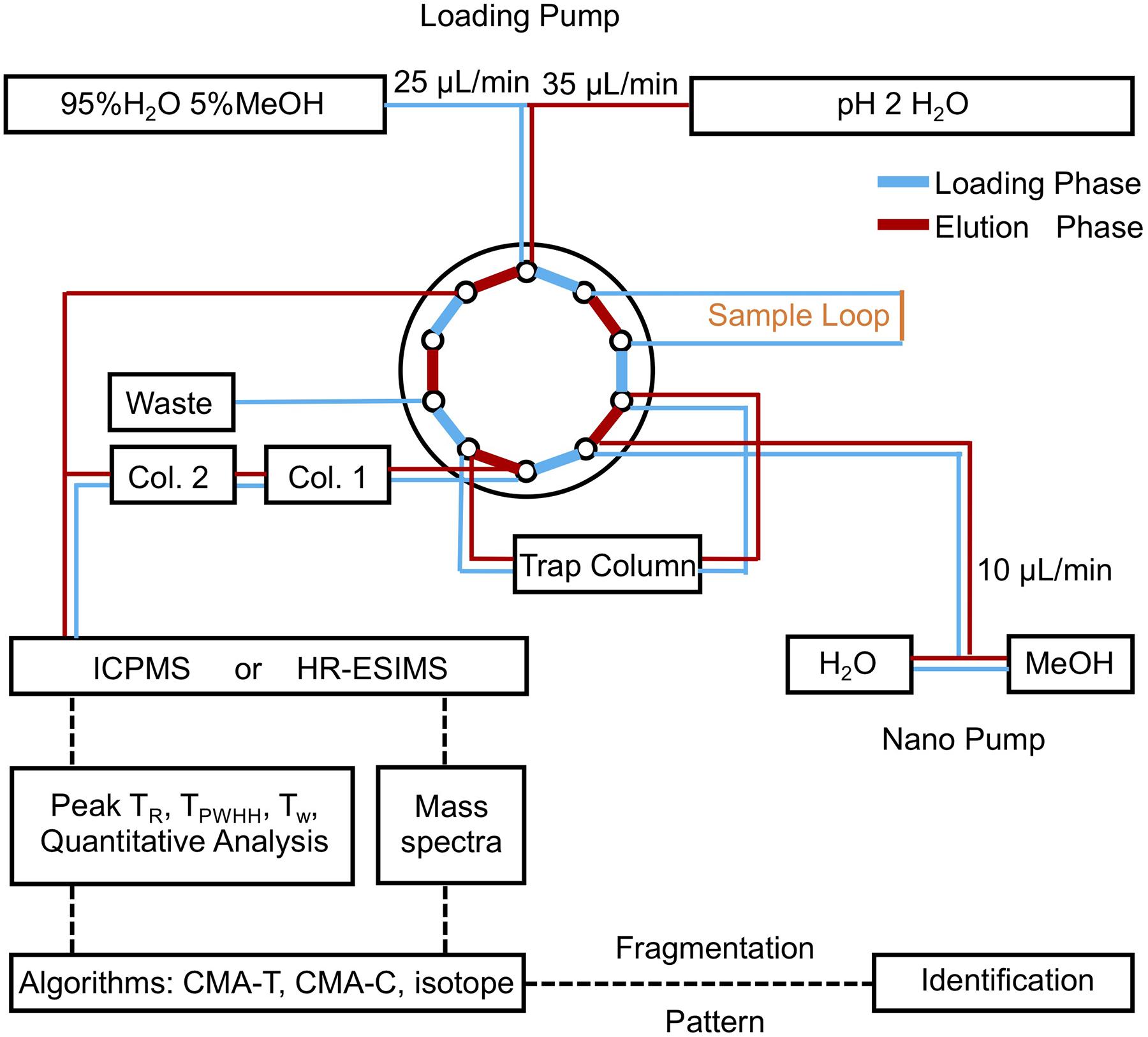
Figure 2. Schematic of the low-flow/make-up flow LC-MS instrumentation. Samples are picked up by the injector and loaded onto the trap column by the loading pump. Once loading is complete, the 10 port-valve switches to the nano-pump, which pushes the sample onto the columns, and elutes it using a gradient of aqueous methanol. During the elution phase, the loading pump flow is redirected to deliver a make-up flow that is post column infused, before entering ICPMS. The LC-ICPMS data are used to target nutrient metabolites by retention time and peak width. Companion ESIMS data are then queried by algorithms to assign masses, elemental formula, and MS² spectra of nutrient metabolites.

As described in the discussion, for the Prochlorococcus sample, the liquid chromatography separation before ICPMS and ESIMS was performed in two modes, resulting in four LC-MS runs for one sample. For the first separation we used a C18 column (3 μm, 2.1 × 150 mm, Hamilton PN 79641), and directed the effluent to ICPMS and ESIMS. Then, for the second separation we used an RP-Amide column (2.7 μm, 2.1 × 150 mm, Supelco PN 53914-U) and directed the effluent to ICPMS and ESIMS. With each column, samples were separated with a 60 min gradient from 95% solvent A (5 mM aqueous ammonium formate) and 5% solvent B (5 mM methanolic ammonium formate) to 95% solvent B, with 120 μL/min flow rate delivered by the loading pump.

Inductively Coupled Plasma Mass Spectrometry

The combined flow from LC was analyzed using a Thermo Scientific iCAP Q quadrupole mass spectrometer fitted with a perfluoroalkoxy micronebulizer (PFA-ST, Elemental Scientific), and a cyclonic spray chamber cooled to 4°C. Measurements were made in kinetic energy discrimination (KED) mode, with a helium collision gas flow of 4–4.5 mL/min to minimize isobaric ⁴⁰Ar¹⁶O+ interferences on ⁵⁶Fe. Oxygen was introduced into the sample carrier gas at 25 mL/min to prevent the formation of reduced organic deposits onto the ICPMS skimmer and sampling cones. Isotopes monitored included ⁵⁶Fe (at an integration time of 0.05 s), ⁵⁷Fe (0.02 s) and ⁵⁹Co (0.02 s).

Electrospray Ionization Mass Spectrometry

For LC-ESIMS analysis, the eluant from the LC, without qH₂O infusion, was coupled to a Thermo Scientific Orbitrap Fusion mass spectrometer equipped with a heated electrospray ionization source. ESI source parameters were set to a capillary voltage of 3500 V, sheath, auxiliary and sweep gas flow rates of 5, 2, and 0 (arbitrary units), and ion transfer tube and vaporizer temperatures of 275°C and 20°C. MS¹ scans were collected in high resolution (450K) positive mode. The MS² scans were collected, but will not be discussed in the present study. LC-ICPMS and LC-ESIMS data are available as a MassIVE dataset¹ (accession MSV000086964). LC-ICPMS and LC-ESIMS data for the process blank of the North Pacific sample are available as a MassIVE dataset MSV000087149).

Data Analysis and Workflow

The LC-ESIMS data was converted from raw file format to mzXML (MSconvert, ProteoWizard). The mzXML is imported to Matlab, where m/z and intensity from each scan are extracted, and ordered by scan number into a scan number/m/z/intensity matrix, which is then interrogated by mass search algorithms. In the first algorithm, the 3D matrix is cut to discard data beyond the time window defined by the retention time of peaks of interest targeted by LC-ICPMS. The matrix is then binned to generate thousands of extracted ion chromatograms (EIC). Each of the EIC is classified as either a target ion that shows a well-shaped peak, or noise with no defined peak. In the second algorithm, the matrix is binned, and pairs of EICs are registered as ¹²C-¹³C isotopologues if their m/z differ by 1.003 D, and their abundances differ by R, where R is defined by their m/z. Collectively, these two algorithms detect features, either as targeted ions, or as pairs of EICs.

Results and Discussion

Improvements in LC-ICPMS Detection of Metabolites

Nutrient metabolites often occur at nano- to femto-molar concentrations in marine samples, making sensitivity and detection limits key concerns in method design. There are several avenues through which analyte detection limits can be increased. First, samples can be concentrated before LC-MS analysis. However, most SPE protocols used to extract metabolites from seawater trap organic matter with a wide range of polarities. This poses a problem for the next step of sample processing in which the volume of the extract is reduced for chromatographic analysis. When SPE extracts (typically ∼ 5–6 mL) are concentrated to <500 μL (≥10× concentration factor), we often observe the formation of precipitates. Further concentration does not yield a homogeneous extract, limiting the extent to which a reduction in sample extract volume can be used to increase sensitivity. A second approach is to increase injection volumes, chromatographic resolution, and signal sensitivity. In our original method, injection volumes were ∼ 20 μL for standards and ∼50 μL (∼10% of total sample extract) for samples, and we used a conventional analytical flow column with a 2.1 mm inner diameter eluted at a flow rate of 200 μL/min. Injection volumes > 50 μL increased dispersion in the column and decreased chromatographic resolution and reproducibility. However, we found 200 μL/min of high organic solvent content flow into the ICPMS destabilized and often quenched the plasma. We investigated the relationship between the flow rate of high organic solvent content and plasma stability and found a stable plasma could be achieved at 40–50 μL/min of 95% aqueous methanol. We provisionally addressed this problem by adding a post-column splitter to our system to direct 80% of the 200 μL/min eluent to waste and 20% to the ICPMS. This gave a reliably stable plasma, but resulted in substantial loss of sample.

When samples are directly injected into the ICPMS, a significant two to threefold decrease in the counts of iron and cobalt (and presumably other elements) was observed, for the same compound dissolved in methanol versus water (Boiteau et al., 2013). For metabolites such as siderophores, which display a wide range of polarities and elute across the entire chromatogram, these solvent effects bias quantitative analyses. In the revised method we therefore reduced the size of our chromatographic system further, incorporated an on-line sample trap column to maintain high injection volumes, and added a post-column make-up flow to reduce solvent effects. We use a loading pump to push ∼100–200 μL of sample onto a trap column. The flow into the trap is then switched to a nano pump that elutes the sample at 10 μL/min onto two 0.5 mm ID × 150 mm analytical columns connected in series. Collectively, these columns provide high separation efficiency and resolution. For example, a suite of closely related marinobactins extracted from seawater were efficiently separated from one another by the trap-column/low-flow method (Figure 1). At 10 μL/min, the entire LC eluant can be directed into the ICPMS. We also introduced a post-column make-up flow of 35 μL/min pH 2 qH₂O delivered by the loading pump (Figure 2). The make-up flow improved plasma stability and reduced the change in the organic solvent content of the flow into the ICPMS from 5–95% to 1–21% across the chromatographic run. This smaller fractional change in organic content reduced solvent effects across the analyses. Figure 3 compares the separation and detection of two siderophores using the high-flow and low-flow methods, demonstrating the five-fold greater ICPMS response, and the significantly reduced solvent effects with the low-flow method. In this example the ratio of ⁵⁶Fe peak areas for a 1:1 solution of ferrichrome and ferrioxamine-E applied to the column changed from 1:0.5 without the make-up flow to 1:0.9 with the make-up flow (Figure 3). Particularly for studies where sample amount is limited, the low-flow method offers clear advantages. For the analysis of siderophores in seawater, we were able to reduce the seawater sample size from 20 L to 4 L by adopting the low-flow method.

FIGURE 3

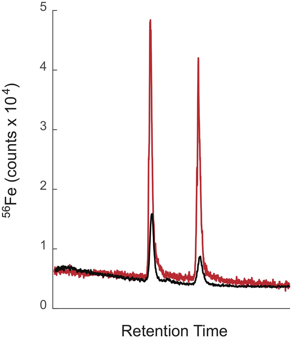
Figure 3. LC-ICPMS Fe chromatograms of ferrichrome and ferrioxamine E (2 nmol each) showing the better sensitivity and decreased solvent effects of the low-flow/make-up flow system (red trace) compared to the high-flow/split system (black trace). The low flow/make-up flow system was eluted with a flow rate of 10 μl/min with a make-up flow of 35 μl/min pH 2 qH2O. The high-flow/split system was eluted with a flow rate of 200 μl/min, which was split post-column with, 20% entering the ICPMS, 80% going to waste.

Nevertheless, even with the low-flow method, we noted a significant drop in the baseline detection of iron with increasing percentage of solvent B (Figure 4). We attributed the decrease in baseline ⁵⁶Fe counts to either: (1) a direct decrease in ICPMS sensitivity due to less efficient atomization and ionization by cooling of the central channel of the ICPMS plasma (Hu et al., 2004) when organic solvents are sprayed into the plasma chamber, or (2) a decrease in the amount of Fe contamination delivered to the ICPMS from either a lower level of contamination in, or a lower level of Fe leaching from the stainless steel LC column jacket by the organic solvent (here LC-MS grade methanol redistilled in Teflon to reduce trace metal contamination) compared to qH₂O (solvent A). In the original method of Boiteau et al. (2013), siderophores were quantified by multiplying the baseline-corrected peak area by an ICPMS response factor for Fe derived from a plot of peak area vs amount for ferrichrome and ferrioxamine-E standards. If the drop in baseline Fe counts results from less Fe contamination in solvent B, it would be fully accounted for by baseline correction, and the quantification of siderophores would be accurate. In contrast, if the sensitivity of the ICPMS for Fe decreases due to direct solvent effects on the plasma, baseline correction alone would underestimate the concentration of siderophores eluting later than the calibration standards. To distinguish and quantify these two effects, we added 10 ppb ⁵⁶Fe in pH 2 qH₂O to the make-up flow. This is 50 times higher than the amount of iron represented in the baseline of a typical analysis, so changes in iron contamination from the LC solvents or from contamination from the LC column were negligible. In this experiment, the ⁵⁶Fe delivered to the ICPMS was effectively constant over the course of the experiment. Changes in baseline ⁵⁶Fe detection were therefore attributed only to change in ⁵⁶Fe detection by the ICPMS. We chose 40 min, which lies between the retention times of ferrichrome and ferrioxamine-E (the siderophores used to calibrate our measurements) as a reference point for our comparison.

FIGURE 4

Figure 4. LC-ICPMS ⁵⁶Fe-chromatogram of ferrichrome and ferrioxamine E (200 fmol each), with a make-up flow of 35 μl/min pH 2 qH2O (red trace). To measure the effect of solvent B on the detection of iron, we performed an identical analysis, but added 10 ppb ⁵⁶Fe to the make-up flow (gray trace). Iron delivered to the ICPMS in this analysis was dominated by the 10 ppb infusion and was effectively constant over time, making the ⁵⁶Fe counts a good proxy of Fe sensitivity by ICPMS. A linear regression of ⁵⁶Fe-counts and time (black solid dashed line) gives a good fit to the data with %Fe = –0.88 (retention time (min))+136.08% with r² = 0.99. For the comparison here, each 56Fe-chromatogram, was normalized to the ⁵⁶Fe counts at 40 min, the average retention time of the two standards.

The results are shown in Figure 4. Even with constant delivery of ⁵⁶Fe to the ICPMS, the normalized baseline counts (%) for ⁵⁶Fe drop from 100% to 55% between 40 and 80 min. We attribute all of this decrease (45%) to the impact of solvent composition (%water to %methanol) on the ICPMS sensitivity for ⁵⁶Fe. In comparison, when the ferrichrome and ferrioxamine mixture was analyzed without iron added to the make-up flow, the baseline between 40 and 80 min drops from 100 to 25% Of the 75% drop in signal, most of the decrease in signal (45%) was attributed to the direct solvent effect, while a lesser amount (30%) was attributed to changes in ⁵⁶Fe contamination delivered to the ICPMS from the LC hardware and solvents. When 10 ppb Fe is delivered by the make-up flow, a linear regression of ICPMS counts with retention time yields a good fit for the 20–100 min time window (Figure 4), allowing accurate correction for direct solvent effects on the ICPMS for most every peak in a typical sample chromatogram. Likewise, we can correct for solvent and LC hardware contamination by baseline subtraction of a sample blank. We note that ⁵⁶Fe contamination by solvents and LC hardware will change with analytical conditions; using solvents direct from the supplier (without distillation in a PTFE still as was used here) may increase contamination while using PEEK lined LC column jackets may decrease it. Finally, we noted that sample matrix effects, the effects of co-eluting organic compounds in the sample, often affect the ionization efficiency of iron (and presumably other elements). These effects are not corrected by baseline subtraction or adjusting the ICPMS response factor for solvent B content. To correct for matrix and solvent effects, we added ¹¹⁵Indium to the make-up flow with the intention of using this rare isotope as an internal calibrant for changes in ICPMS sensitivity in each sample. However, we found small differences in the response of ICPMS sensitivity for ⁵⁶Fe that did not match those measured by ¹¹⁵In, and we set aside any further investigation of this approach. Incorporation of a ⁵⁷Fe in place of ¹¹⁵In could be used to correct the ICPMS response to iron, but internal calibration standards may have to be element specific.

Mass Search Algorithm I: Compound Mass Assignment-Time (CMA-T)

Iron-ligand complexes detected by LC-ICPMS are identified or characterized by analyzing the sample a second time with ESIMS detection. To assign masses to Fe ligand complexes, Boiteau and colleagues (Boiteau et al., 2016, 2019) applied a mass search algorithm that queries the ESIMS dataset for co-eluting isotopologues for iron, copper and nickel. For iron, the algorithm searched for ⁵⁶Fe- and ⁵⁴Fe-containing ion pairs with a mass difference of 1.995 ± 0.002 D and abundance ratio of 15.7 ± 4.7. The approach implicitly assumed that the iron isotopic composition is crustal (15.7). This was a good assumption for some laboratory cultures of siderophore producing microbes (Boiteau and Repeta, 2015) and for seawater (Boiteau et al., 2016; Bundy et al., 2018). However, for some cultures of marine cyanobacteria and for some environmental samples we found a substantial deviation in R from the crustal ⁵⁶Fe:⁵⁴Fe ratio, possibly due to isotopic fractionation during complexation or uptake. In these cases, the algorithm returns false negative results and fails to find masses for Fe-Ls from ESIMS data that are clearly visible in the ICPMS data. Of greater importance, many nutrient metabolites of interest incorporate elements such as cobalt, manganese, iodine, or phosphorus that do not have abundant stable isotope pairs and therefore are not amenable to discovery through our original algorithm.

To address this, we developed two new simple algorithms for feature detection. A feature is a two-dimensional signal (intensity vs. retention time) of a specific m/z that includes one or multiple peaks. Features can be caused by either organic compounds or instrument noise. These two algorithms are collectively named compound mass assignment (CMA) based on time (CMA-T) or carbon (CMA-C) and can be used singularly or in combination.

Annotated code for CMAs (written in Matlab) are available through github². To demonstrate the CMA-T algorithm, we used it to assign peaks in the ICPMS Fe-chromatogram of siderophores extracted from spent media from a laboratory culture of V. cyclitrophicus strain 1F-53. We selected the starred peak in the LC-ICPMS chromatogram shown in Figure 5 as our “unknown” target. We then defined a time window (T_w) centered at the peak’s retention time (T_R; here 5063 s) as T_w = [(T_R-NT_PWHH), (T_R+NT_PWHH)], where T_PWHH represents the peak width in time at half height (code line 62-64). Both T_R and T_PWHH were determined from the LC-ICPMS chromatogram. The positive integer N specifies the overall size of the time window used, and is set by the analyst. The value of T_w is adjustable with peak width (T_PWHH), which may change with retention time, and with N, which is set depending on the complexity of the chromatogram. Here T_PWHH = 30s, and we set N = 3, generating a T_w of 180 s [4973 s, 5153 s]. In practice we found that with the gradient used for our siderophore analyses, setting T_PWHH = 15–30 s, N = 3–6 and therefore T_w = 90–360 s as constants works for most searches.

FIGURE 5

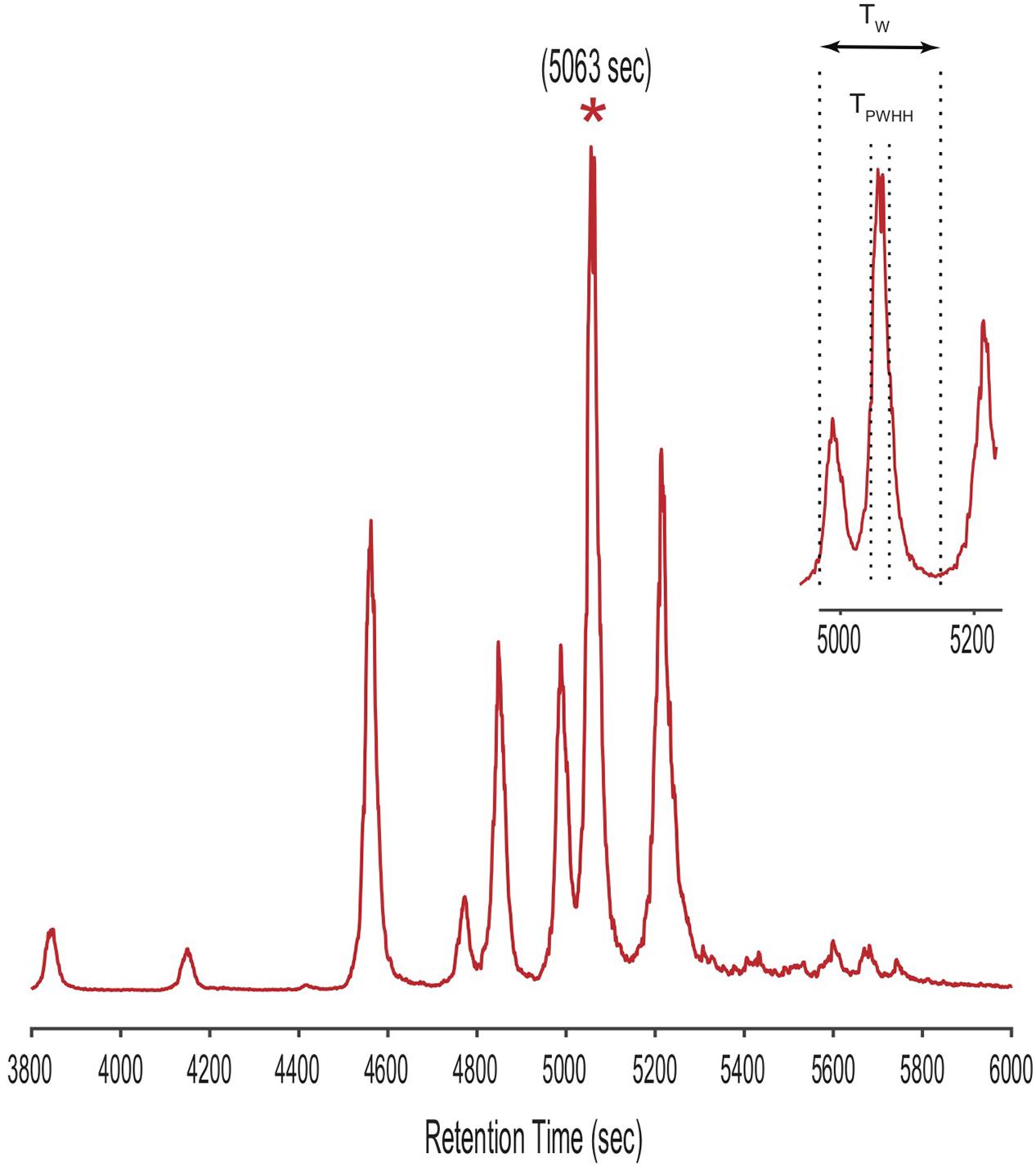
Figure 5. LC-ICPMS Fe-chromatogram of the SPE organic extract of V. cyclitrophicus strain 1F-53 culture media after addition of iron. The starred peak (*) was selected as our unknown target metabolite to illustrate the application of CMAs. The insert shows the definition of the time window (T_w) in the CMAs, as determined by the retention time (T_R = 5063s) and the peak width at half height (T_PWHH).

The sample is analyzed again on LC-ESIMS, the dataset is aligned using the retention time of an internal standard (here Ga-desferrioxamine E, which can be obtained by monitoring m/z of 667.26 on ESIMS and ⁶⁹Ga on ICPMS, code line 31). Next, the LC-ESIMS mass intensities between 500 and 1000 D within this T_w were binned by 0.01 D increments, which is well below the mass resolution of the spectrometer (m/Δm = 450,000 at 200 m/z) for this mass range (code line 72). This mass range encompasses most known siderophores, but can be customized to search for any mass window. It is noteworthy that finer binning size could be used, which would provide greater mass accuracy, but also an increase in processing time.

Binning generated thousands of extracted ion chromatograms (EIC). Each EIC was assigned as either a target ion or as noise (code line 72-117). To distinguish the two we define a function as the square of the intensity (I²) for each ion in the ESIMS data, and integrate the function over time. For compounds that elute from the LC column as Gaussian-shaped peaks, the integral of I² over time increases rapidly, ascending from 5% to 95% of its integral total in < 0.2T_w. In contrast, for ions that appear as noise, the integral of I² has as a slow and stepwise increase, rising from 5 to 95% in > > 0.2T_w. Therefore, we can use 0.2T_w as the threshold to distinguish EICs of target ions from noise (Eq. 1, Figure 6).

FIGURE 6

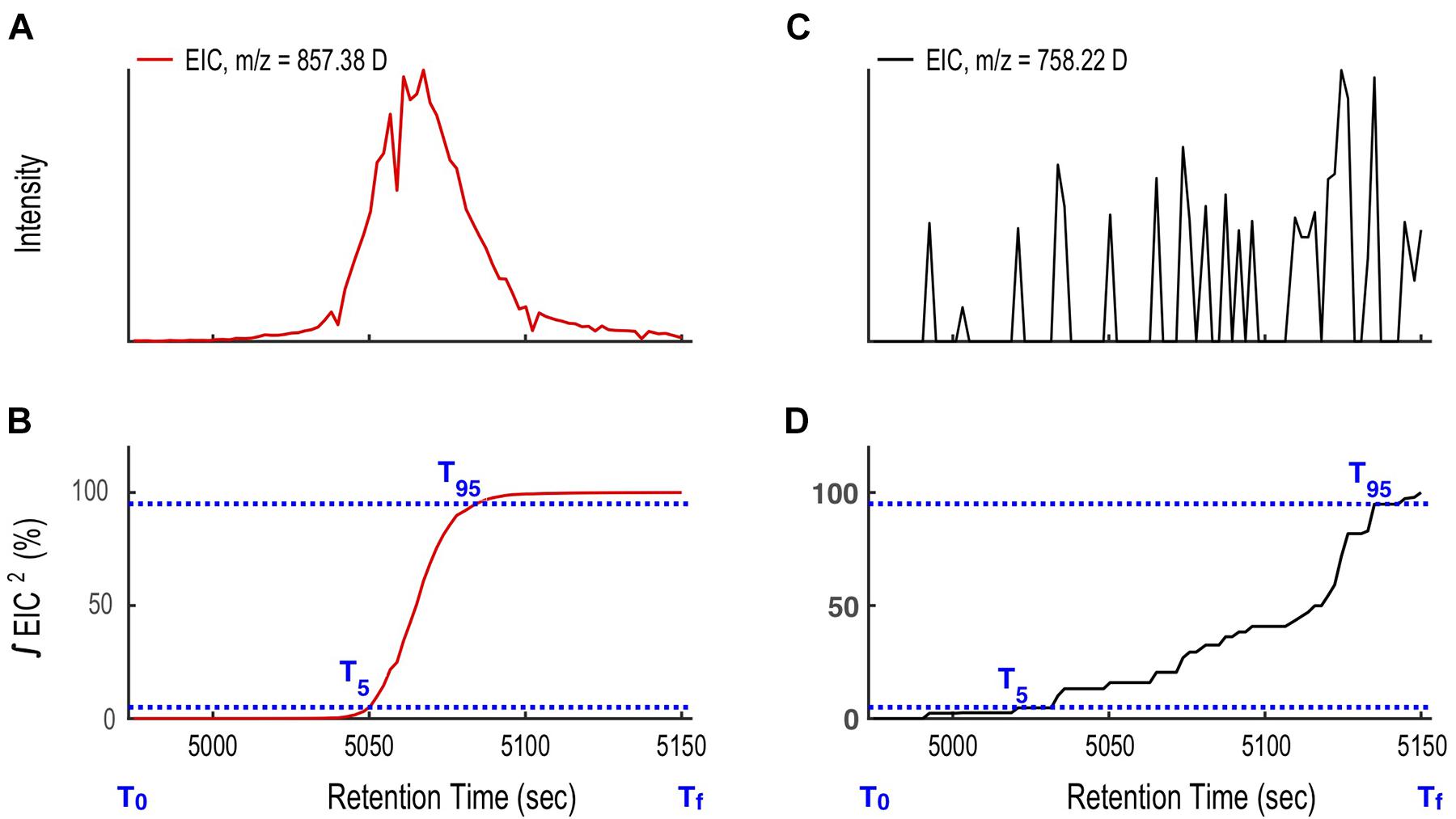
Figure 6. Illustration of the compound mass assignment-time (CMA-T) algorithm. (A) The ion at 857.38 D targeted by CMA-T has the rise and fall in intensity with time expected for a well-shaped peak eluting from the LC. (B) The integral of the square of the 857.38 D ion intensity (I²) over time ΔT (T₉₅-T₅) rises from 0.05% (T₅) to 0.95% (T₉₅) of its total value in ΔT ≤ 0.2T_w. (C) Ions that arise from noise show a more gradual rise and fall in intensity over time, and (D) for the same ΔT, the integral of I² between T₅ to T₉₅ ≥ 0.2 T_w. The comparison between ΔT (T₉₅-T₅) and 20% T_w is used as a filter to differentiate target ions from noise.

$$TargetIon:T95-T5\le 0.2Tw;$$

$$Noise:T95-T5>0.2Tw;$$

$$where\underset{T0}{\overset{T5}{\int }}{I}^{2}dt=0.05\underset{T0}{\overset{Tf}{\int }}{I}^{2}dt;\underset{T0}{\overset{T95}{\int }}{I}^{2}dt=0.95\underset{T0}{\overset{Tf}{\int }}{I}^{2}dt;$$

$$T0=4973sec,;Tf=5153sec;Tw=Tf-T0=180sec$$

After applying CMA-T, two additional filters are applied as a quality control step to remove false positive peaks. First, for each ion, if 50% or more of the ESIMS scans within T_w show zero counts, it is removed from the target list (code line 88-109). This eliminates any well-shaped peaks that are poorly or partially captured by the defined time window (Figure 5). In this example, we collected 80 scans across T_w, so a target ion must include at least 40 non-zero data points. Second, if the peak center (maximum in intensity) of its EIC is > T_PWHH from T_R, it is removed from the target list (code line 104-106). This eliminates peaks that are significantly shifted in retention time between LC-ICPMS and LC-ESIMS analysis, which is not expected after spectra alignment. When we applied CMA-T with T_R = 5063 s, T_PWHM = 30 s, T_w = 180 s and a threshold value of ≥40 data points to the ESIMS data from the Vibrio culture media extract, the algorithm identified 12 EICs as target ions that elute within this time window (Figure 7).

FIGURE 7

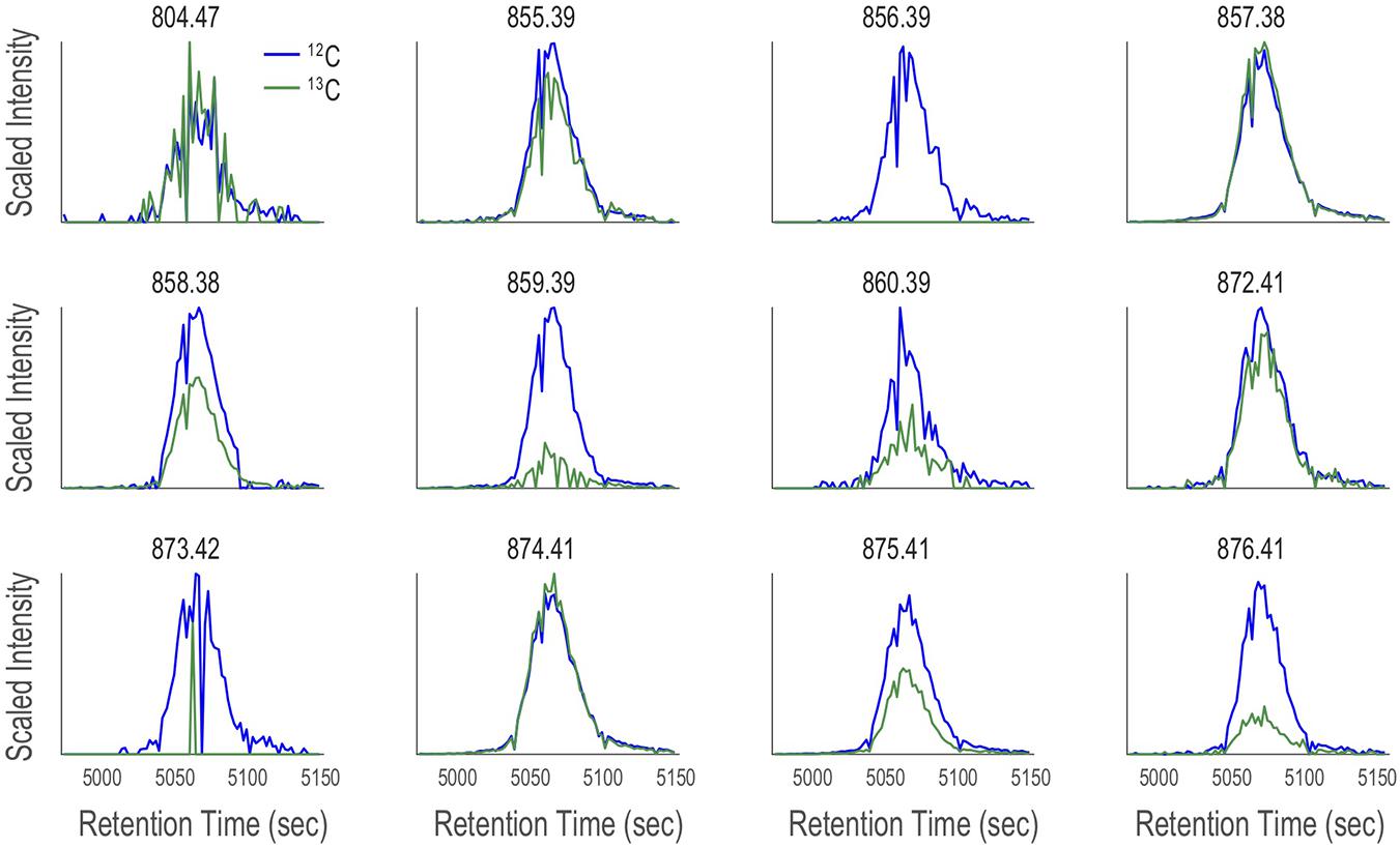
Figure 7. Twelve target ions discovered by CMA-T that elute within T_w = 4973–5153 s in the SPE organic extract of V. cyclitrophicus strain 1F-53 culture media after addition of iron. The EIC of each target ion (M; blue traces) is overlaid with the EIC of (M+1.003; green traces), after scaling the latter by the relative abundance of ¹³C calculated according to Figure 8, under the assumption of a singly charged ion and 50% carbon content.

Mass Search Algorithm II: Compound Mass Assignment-Carbon (CMA-C)

Spurious noise or co-eluting peaks can yield false positive target ions after the CMA-T algorithm filter. These can be removed by processing the ESIMS data with CMA-C. Originally, CMA-C was designed to find all the organic compounds with a defined fraction of carbon within any given time window, by searching for pairs of isotopologues containing exclusively ¹²C (M peak) and one ¹³C (M+1 peak) atoms. This approach is similar to our original mass search algorithm that searches for ⁵⁶Fe-⁵⁴Fe isotopologues (Figure 1). In that algorithm, a pair of EICs are attributed to an Fe-containing compound if their m/z differ by 1.995 D, and their intensities differ by 15.7. In CMA-C, a pair of EICs is attributed to a C-containing compound if their m/z differ by 1.003 D, and their intensities differ by a ratio R. The ratio R in CMA-C is a dynamic parameter, determined by the number of carbon atoms in the compound, which can be estimated by the m/z of the EIC, and the fractional weight of carbon in the compound (code line 43-65). The fractional weight of C in siderophores extracted from a database of 366 known siderophores (Baars et al., 2014), is 48% + 5%, so that for a siderophore of mass m, R = [(0.5)(0.011)(m/z)/(12)], where 0.5, m/z, 0.011 and 12 represent the average carbon content of known siderophores, mass to charge ratio for the target ion, relative abundance of ¹³C (slope in Figure 8), and atomic mass of ¹²C respectively.

FIGURE 8

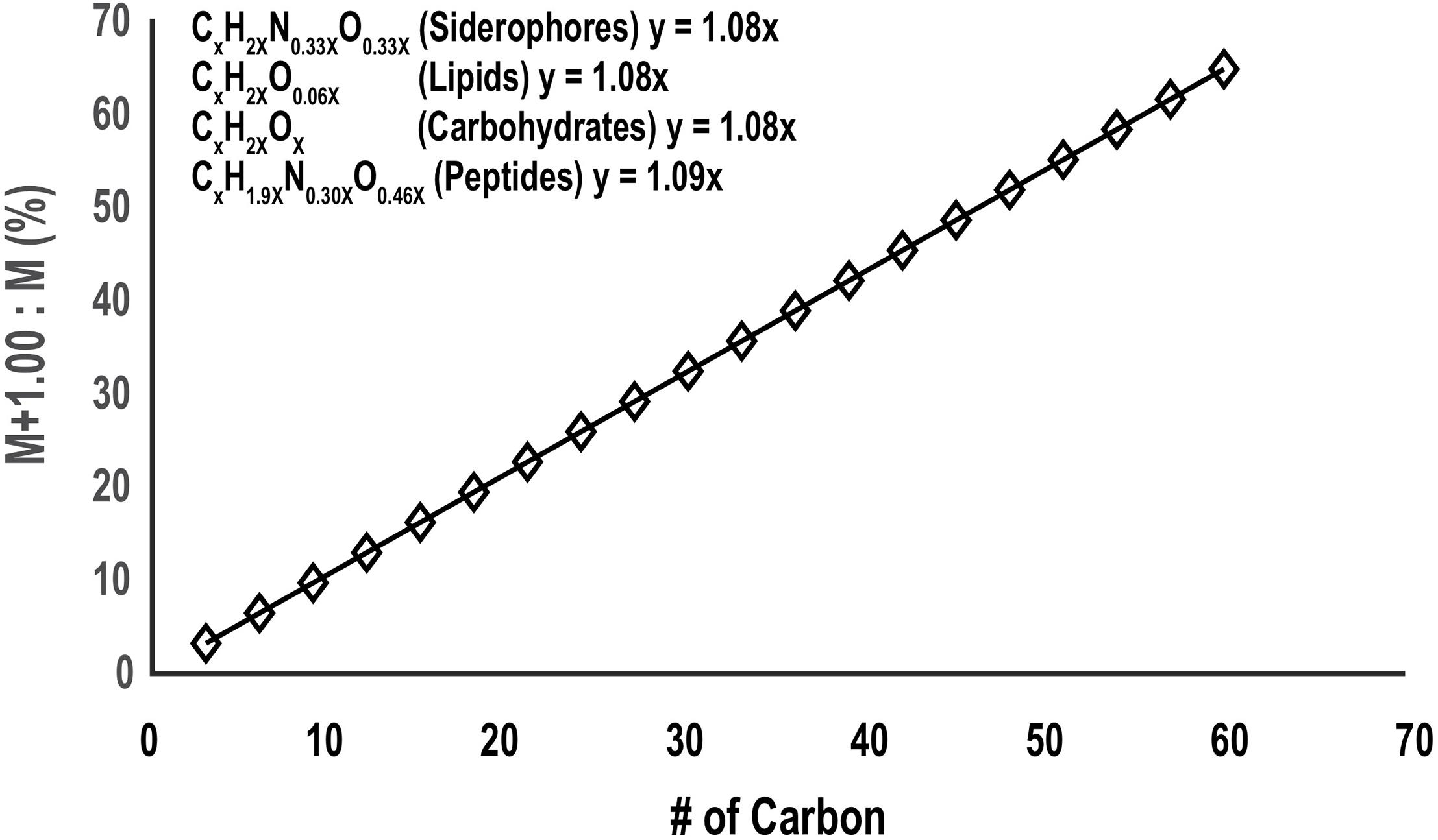
Figure 8. The relative abundance of the ¹³C:¹²C isotopologue molecular ions (M+1.00/M) as a function of carbon number for siderophores, lipids, carbohydrates, and proteins (the molecular formula is extracted from Rivas-Ubach et al., 2018). Although these classes of metabolites are different in the ratio of H, N, and O they incorporate relative to C, the change in carbon isotopic ratio with carbon number between them is very small and for the mass search algorithms the ratio can be approximated by the slope of the plot (1.08).

Although CMA-C can be used independently to generate a list of targeted ions, we here use this algorithm to query the targeted ions by CMA-T. For example, the ¹³C isotopologue for the target ion 857.38 D will have a mass of 858.38 D and an intensity of 39% of the target ion (857.38 D). We overlaid each of the 12 EICs with the plot of EIC+1.003 (the difference in mass between ¹²C and ¹³C), and scaled the plot by the relative abundance of ¹³C calculated as described above. If the target ion is from a singly charged organic compound, the two EIC should overlay each other closely. Here we assume the ion of interest is singly charged, however, other charge states can be assumed as described in Section “Application II: Targeting Monoisotopic-Element Nutrient Metabolites Using Multi-Dimensional Chromatography With Mass Search Algorithms” for cobalt-containing metabolites. If the target ion has a carbon content significantly different from 50%, is multiply charged, or if the target ion itself is the ¹³C isotopologue of a peak captured by CMA-T, the two plots will track each other in time, but will be offset in scaled intensity. Finally, if the two plots do not track each other in time or scaled intensity, the target ion is regarded as a false positive.

We used the CMA-C algorithm to query the 12 target ions assigned by CMA-T to the Fe-chromatogram peak at 5063 s. Five of the 12 target ions passed the CMA-C filter: 804.47 D, 855.39 D, 857.38 D, 872.41 D, and 874.41 D. From the differences in mass between pairs of ions, we can easily assign four of these target ions as the ⁵⁴Fe:⁵⁶Fe isotopologue pairs of the ion with m/z = 855.39 and 857.38 D (⁵⁴Fe m/z_obs = 855.386, m/z_thero = 855.388, ⁵⁶Fe m/z_obs = 857.382, m/z_thero = 857.383 D) and its ammonium adduct at m/z = 872.41 and 874.41 D (⁵⁴Fe m/z_obs = 872.412, m/z_thero = 872.415, ⁵⁶Fe m/z_obs = 874.408, m/z_thero = 874.410 D). A search of our database of known siderophores identified the compound as Amphibactin-T. The ion at 804.47 D has a Δm = 52.912 D less than the Amphibactin-T ion (m/z_obs = 804.470, m/z_thero = 804.472); and arises from nonmetallated (apo-; -Fe+2H) form of the siderophore.

For the seven ions that are rejected by CMA-C, four (856.39 D, 858.38 D, 873.42 D and 875.41 D) represent the ¹³C isotopologue of Amphibactin-T and its ammonium adduct. Similarly, the target ions 859.39 D and 876.41 D may contain either additional ¹³C atoms, or an ¹⁸O atom on top of 857. 38 D and 874.41 D. Furthermore, 860.39 D may contain both a ¹³C atom and an ¹⁸O atom on top of 857. 38 D. These isotopically rare compounds are low in relative abundance, but could be detected when the overall concentration is high, as demonstrated in this example. In summary, the CMA-C returns only the major isotopologue (¹²C-¹H-¹⁶O-¹⁴N-, etc.) of a compound. The combination of CMA-T and CMA-C was able to correctly identify the molecular ions of Amphibactin-T from the ICPMS and ESIMS data without using isotopes of iron in the search algorithms.

Application I: Targeting Monoisotopic-Element Metabolites in Environmental Samples

In the sections above, we treated Fe as a “monoisotopic” nutrient, and successfully assigned masses to siderophores in laboratory culture samples. Here, we use the algorithms to assign the mass of a siderophore complexed to aluminum in an environmental sample. Aluminum is monoisotopic, and in the +3 oxidation state aluminum forms stable complexes with some siderophores. Although siderophore-Al complexes have lower binding constants than siderophores complexed to iron, Al is ∼10× more abundant than iron in surface seawater, therefore, many environmental samples that contain siderophores also contain siderophores complexed to aluminum. For example, the ²⁷Al-chromatogram for the North Pacific seawater sample shown in Figure 1 looks similar to that of ⁵⁶Fe. Specifically, it displays four major peaks eluting between 70 and 82 min. We targeted the ²⁷Al peak at 80.6 min (4837 s) for mass assignment.

When we applied CMA-T to the ESIMS data from the North Pacific Seawater extract with following parameterization: T_R = 4837 s, T_PWHM = 30 s, N = 5, T_w = 300 s, mass window = 500–1100 D, data points in the peak ≥ 20, and T₉₅-T₅ ≤ 0.1 T_w, the algorithm identified 18 EICs as target ions that elute within this time window. We then used the CMA-C algorithm to query these target ions, assuming a carbon fractional weight of 30–70%, which was selected based on the carbon content of siderophores (48% +5%).

Two of the 18 EICs identified by CMA-T passed the CMA-C filter: 984.482 D and 1013.434 D. From the differences in their mass (28.952 D), and the presence of a co-eluting peak in the ²⁷Al and ⁵⁶Fe-chromatograms, we can easily assign the two ions as an ²⁷Al-siderophore and an ⁵⁶Fe-siderophore. A search of our database of known siderophores identified the two compounds as Al-marinobactin-C (m/z_thero = 984.483 D), and Fe-marinobactin-C (m/z_thero = 1013.437 D).

Application II: Targeting Monoisotopic-Element Nutrient Metabolites Using Multi-Dimensional Chromatography With Mass Search Algorithms

For nutrient metabolites that have monoisotopic elements (with respect to stable isotopes), the application of CMA-T and CMA-C filters alone may be insufficient to identify the molecular ion of a compound targeted by ICPMS. This would happen when multiple ions, which could not be easily related to each other or to a known metabolite, are returned by CMAs. To make these assignments we took advantage of changes in compound selectivity under different chromatographic conditions. Changes in either the mobile (solvent) or stationary (column packing material) phases will move compounds into or out of a particular time (T_w) searched by the algorithms. We expect that compounds co-eluting with a compound targeted by LC-ICPMS, and therefore the suite of ions targeted by CMA-T and CMA-C, will change with chromatographic conditions. To demonstrate this approach, we created a “Prochlorococcus sample” by adding cobalamin (vitamin B₁₂) to the SPE extract of spent media from a laboratory culture of the marine cyanobacterium Prochlorococcus MIT9215. We note that the media used for this culture was prepared by amending natural seawater with nutrients, so that the “Prochlorococcus sample” contains the natural suite of organic matter typically extracted from Sargasso seawater along with organic matter produced by Prochlorococcus during growth. Our goal was to determine if the intersection of target ions generated by CMA-T applied to a sample separated using two different chromatographic conditions would identify the correct molecular ion (here m = 1356.58 D) for a metabolite incorporating cobalt, a monoisotopic element.

The Prochlorococcus sample was first analyzed by LC-ICPMS and LC-ESIMS fitted with a C18 column (see Methods). The LC-ICPMS trace shows a cobalt-containing compound at 1832 s (Figure 9A). ESIMS data were collected between 300 and 1800 D and binned in 0.01 D increments. CMA-T was applied to the ESIMS data with T_R = 1832 s, T_PWHH = 15 s and N = 3, identifying 10 target masses (Figure 10 and Table 1) as potential molecular ions for cobalamin. We then repeated the analyses but replaced the C18 columns with an amide column, which we expected to have a different selectivity of compounds eluting within T_w. The LC-ICPMS Co-chromatogram again shows a single peak for Co, but at a retention time of 1461 s (Figure 9B). After generating the complement LC-ESIMS data with the amide column, we applied CMA-T with T_R = 1461 s and T_PWHH = 15 s and N = 3, and found 19 target ions that elute within T_w (Table 1).

FIGURE 9

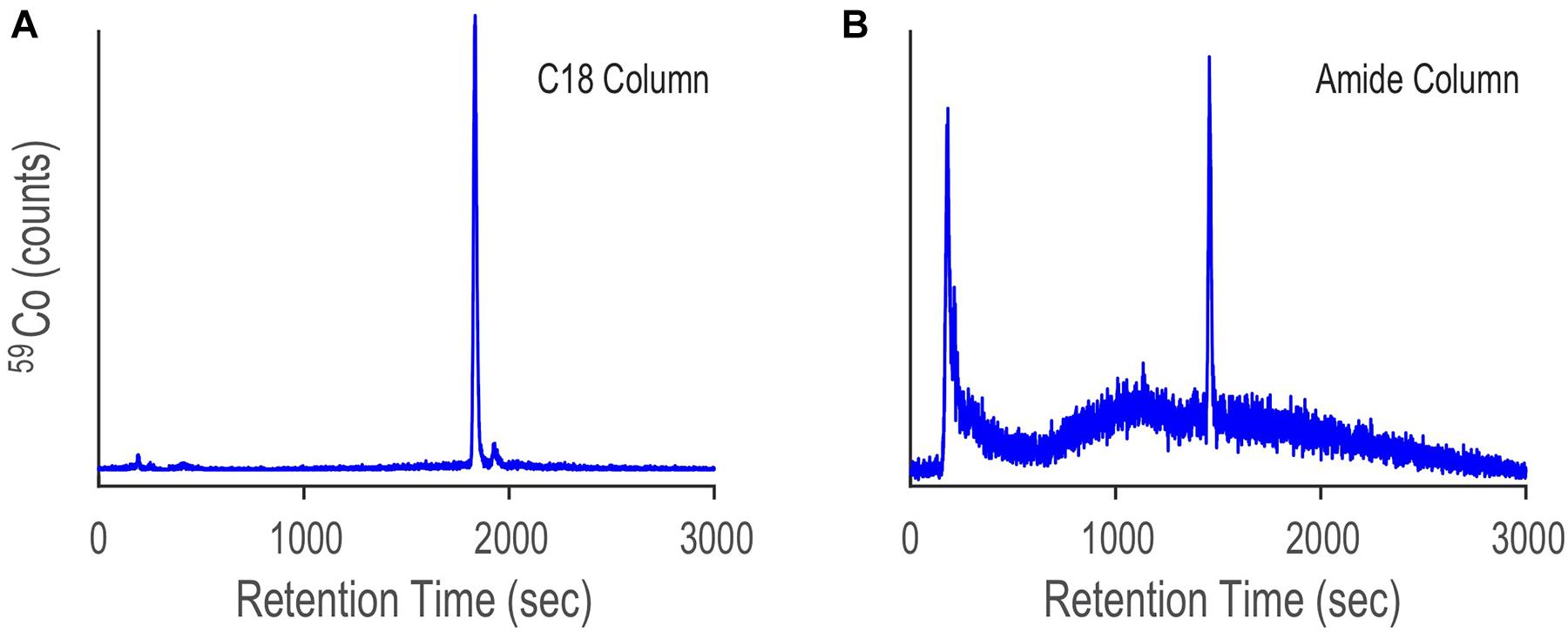
Figure 9. LC-ICPMS Co-chromatograms of the SPE organic extract of Prochlorococcus MIT9215 culture media, separated with a C18 column (A) and an amide column (B). The large peak in both chromatograms is due to the elution of the cobalamin spike. The difference in cobalamin retention time between the two separations is due to the change in selectivity of each column.

FIGURE 10

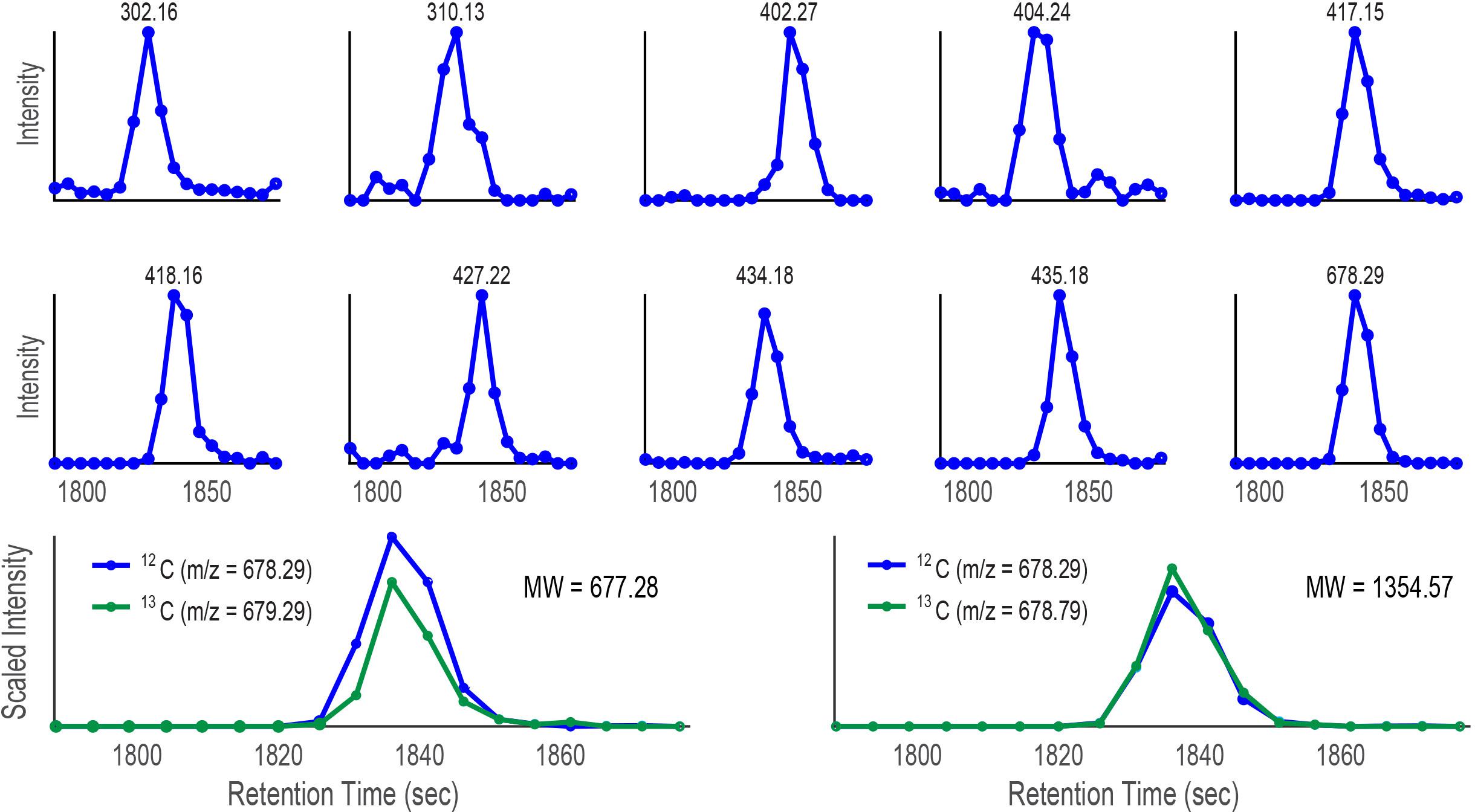
Figure 10. Plots of intensity vs retention time for ten target ions discovered by CMA-T that elute within T_w = 3357–3537 s in the SPE organic extract of Prochlorococcus MIT9215 culture media separated by a C18 column. When the target ion 678.29 D is assumed to be singly charged, CMA-C scales the ion at 679.29 D (green trace; 678.29 D+1.003 D, assumed ¹³C isotopologue) in each scan by a factor of 3.2 which is overlaid with the EIC of 678.29 D (¹²C isotopologue, blue trace) in the lower left of the Figure. When the ion 678.29 D is assumed to be doubly charged, CMA-C scales the ion at 678.79 D (green trace, 678.29 D + (1.003 D)/2 = 678.79 D) in each scan by a factor of 1.6, and overlays the result with the EIC of 678.29 D (lower right). The better fit of 678.79 D plot suggests the ion is doubly charged and that the molecular weight of the ¹²C isotopologue is 1354.57 D.

TABLE 1

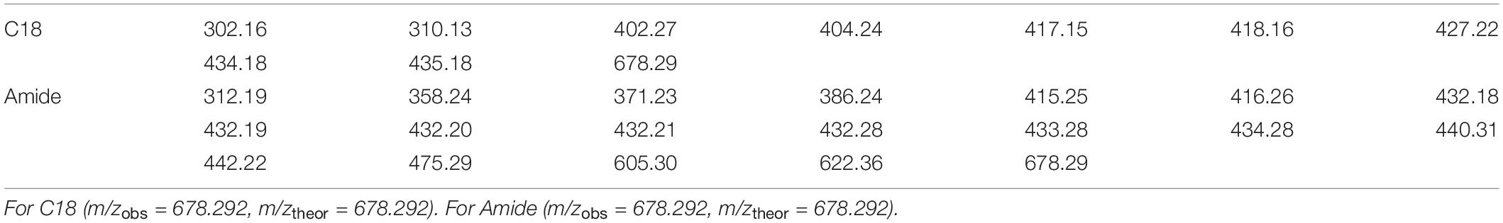
Table 1. Targeted ions (D) found by CMA-T from LC-ESIMS dataset with C18 column and Amide column, with overlapping ion bold in font.

Comparing the CMA-T outputs from the two separations, we found only one common target ion at 678.29 D. We tentatively assigned this mass to the Co-containing compound. Next, we used CMA-C to determine the charge state of the ion. As shown in Figure 10 when the ion 678.29 D is plotted using CMA-C we found the expected carbon isotopic pattern only under the assumption of a +2 charge. Therefore, we conclude that the Co-compound has a molecular weight of 1354.57, which is the mass of the ¹²C isotopologue of cobalamin. CMA-T and CMA-C did not find the singly charged molecular ion for cobalamin because it was not detected by ESIMS; the compound was only ionized as the doubly charged species. In summary, CMA-T and CMA-C, when combined with multi-dimensional chromatography was able to assign the correct molecular ion to a compound (in this case cobalamin) incorporating a monoisotopic element even in a complex mixture of organic matter.

Application III: Characterization of Iodine Metabolites From Prochlorococcus MIT 9215

Marine phytoplankton reduce iodate, the most stable species of iodine in seawater, to iodide (Wong et al., 2002). In doing so they produce a broad suite of organic iodine metabolites that can be detected by LC-ICPMS. Like cobalt, iodine is monoisotopic with respect to stable isotopes, making organic iodine metabolites particularly challenging to characterize.

The Prochlorococcus MIT9215 spent media sample we used to assign the mass of cobalamin in the previous discussion also had a complex suite of iodine metabolites detected as well resolved peaks by LC-ICPMS. The complexity and distribution of iodine metabolites illustrated by the ¹²⁷I chromatogram shown in Figure 11 are characteristic of virtually all seawater and culture media samples we have analyzed to date. Organic iodine metabolites are abundant, diverse, and common in marine samples. The C18- and amide- columns used for our cobalamin analyses show different selectivity for iodine metabolites, as illustrated by the change in iodine distribution across each chromatogram. To investigate iodine metabolites further, we assumed the largest peak in each ICPMS chromatogram was the same metabolite, and targeted this compound for characterization by CMA-T and CMA-C. For the C18 separation, we targeted the ¹²⁷I peak with a retention time of 3447 s, collected ESIMS data between 200 and 1800 D and binned this data in 0.01 D increments. CMA-T was applied to the ESIMS data with T_PWHH = 15 s and N = 6, identifying 29 target masses as potential molecular ions for the iodine metabolite. For the amide column separation, we collected ESIMS data in the same manner, targeted the ¹²⁷I peak at 3630 s and applied CMA-T with T_PWHH = 15 s and N = 6, to find 16 target ions that elute within T_w. Comparing the CMA-T outputs from the two separations, we found only two common target ions at 205.09 D and 279.16 D. These ions were queried by CMA-C and the target ion at 205.09 D was rejected as having insufficient data points in the EIC+1.003 output, leaving the target ion at 279.16 D as the most likely candidate for this metabolite (Figure 11). CMA-C also confirmed this ion was singly charged.

FIGURE 11

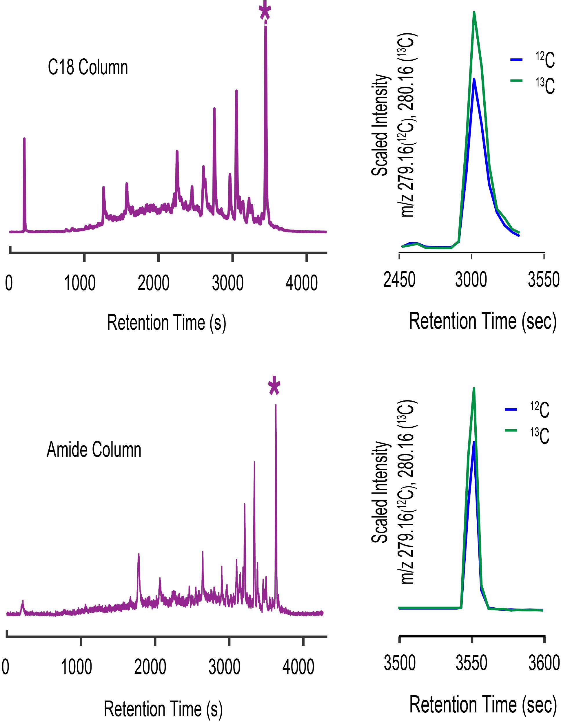
Figure 11. LC-ICPMS ¹²⁷I-chromatogram of organic iodine metabolites in spent media from a culture of Prochlorococcus MIT9215 separated on a C18 column (top, let) and an amide column (bottom, left). The complex mixture of organic iodine metabolites shown in the chromatograms is typical of culture media and seawater samples. When the ESIMS data of the starred (*) peak from each analyses are processed with CMA-T and CMA-C we only find one target ion at 279.16 D (top and bottom, right) that is common to both datasets.

Conclusion

The low abundance of metabolites, and the presence of a complex organic matrix in environmental samples, make the identification and quantitative analyses of metabolites challenging. The element-targeted approach described here offers advantages for characterizing metabolites that incorporate elements other than C, N, H and O. LC-ICPMS allows the analyst to quickly find and quantify these metabolites, while LC-ESIMS allows for their identification or characterization. The approach also assists in defining the elemental composition of a metabolite, which is helpful in applying high resolution mass spectral data to determine elemental formulas. This is particularly useful in targeting metabolites that are involved in biogeochemical cycles of elements such as metals, halogens, and nutrients that have not been previously described due to their low abundance within complex organic samples. In seawater we have detected metabolites that incorporate manganese, copper, nickel, zinc, iodine, and many other elements that, to the best of our knowledge, have not been previously described. Sensitivity is important for enabling the detection of these trace species, and the approach presented here provides a five-fold increase compared to our previous method.

For metabolites that incorporate trace metals, mass search algorithms utilize the mass difference and relative abundance ratio of isotopologues to assign molecular ions (Baars et al., 2014; Boiteau and Repeta, 2015). The CMA-T and CMA-C algorithms described here approach the assignment of molecular ions to ICPMS data somewhat differently. CMA-T only requires that the retention time and peak width of a targeted metabolite are known, and that the peaks are well-shaped. However, metabolites with isomers that have similar retention times might show double peaks on the EIC, which could be classified as noise by CMA-T, resulting in false negatives. CMA-C requires an estimate of the fractional mass of carbon in the class of metabolites of interest, and the algorithm works best for metabolites with > C₁₀, below which the detection of the ¹³C-isotopologue may be compromised, and the carbon content is less predictable. Both CMAs do not require the presence of isotopes (other than for carbon) and can be used with ICPMS, or optical (absorption, fluorescence) detection. For elements with stable isotopes, the combination of an isotope-based mass search algorithm with CMA-T and CMA-C is usually successful in assigning molecular ions to ICPMS data. However, in some cases, particularly for metabolites incorporating monoisotopic elements, the combination of CMA-T and CMA-C alone were often insufficient to assign unique molecular ions. In these instances, we found the most convenient way to make assignments from the suite of target ions identified by the algorithms was to change the separation conditions that determine the masses of co-eluting compounds within T_w until a unique solution is obtained.

Data Availability Statement

The datasets presented in this study can be found in online repositories. The names of the repository/repositories and accession number(s) can be found below: (https://massive.ucsd.edu, accession MSV000086964).

Author Contributions

LB-A and JL revised the LC configuration from the original high flow method to the presented low flow/make-up flow method. JL and ZS designed the algorithms, using mass spectral data provided by LB-A and MA. JL analyzed Vibrio samples. LB-A analyzed Prochlorococcus samples on LC-MS. MM assisted with mass spectral data analyses. JL, RB, and DR wrote the manuscript with assistance from all coauthors. All authors contributed to the article and approved the submitted version.

Funding

This work was generously supported by the National Science Foundation grant OCE-1829761 to RB and OCE-1356747 and -1736280 to DR. DR also received generous support from the Simons Foundation Life Sciences Project Award 49476.

Conflict of Interest

The authors declare that the research was conducted in the absence of any commercial or financial relationships that could be construed as a potential conflict of interest.

Acknowledgments

The authors would like to thank the Captain, crew, and scientific party on the RV Roger Revelle cruise 1814 GEOTRACES GP-15 for sample collection, and Mr. Luis Valentin-Alvarado for providing us with the Prochlorococcus culture. This manuscript is a contribution from the Simons Collaboration on Ocean Processes and Ecology (SCOPE).

Footnotes

1. ^ https://massive.ucsd.edu
2. ^ https://github.com/JingxuanJayLi/RepetaLab

References

Achterberg, E. P., and Van Den Berg, C. M. (1997). Chemical speciation of chromium and nickel in the western Mediterranean. Deep Sea Res. 2 Top. Stud. Oceanogr. 44, 693–720. doi: 10.1016/S0967-0645(96)00086-0

CrossRef Full Text | Google Scholar

Aristilde, L., Xu, Y., and Morel, F. M. (2012). Weak organic ligands enhance zinc uptake in marine phytoplankton. Environ. Sci. Technol. 46, 5438–5445. doi: 10.1021/es300335u

PubMed Abstract | CrossRef Full Text | Google Scholar

Baars, O., Morel, F. M., and Perlman, D. H. (2014). ChelomEx: isotope-assisted discovery of metal chelates in complex media using high-resolution LC-MS. Anal. Chem. 86, 11298–11305. doi: 10.1021/ac503000e

PubMed Abstract | CrossRef Full Text | Google Scholar

Boiteau, R. M., Fitzsimmons, J. N., Repeta, D. J., and Boyle, E. A. (2013). Detection of iron ligands in seawater and marine cyanobacteria cultures by high-performance liquid chromatography–inductively coupled plasma-mass spectrometry. Anal. Chem. 85, 4357–4362. doi: 10.1021/ac3034568

PubMed Abstract | CrossRef Full Text | Google Scholar

Boiteau, R. M., Mende, D. R., Hawco, N. J., McIlvin, M. R., Fitzsimmons, J. N., Saito, M. A., et al. (2016). Siderophore-based microbial adaptations to iron scarcity across the eastern Pacific Ocean. Proc. Natl. Acad. Sci. U.S.A. 113, 14237–14242. doi: 10.1073/pnas.1608594113

PubMed Abstract | CrossRef Full Text | Google Scholar

Boiteau, R. M., and Repeta, D. J. (2015). An extended siderophore suite from Synechococcus sp. PCC 7002 revealed by LC-ICPMS-ESIMS. Metallomics 7, 877–884. doi: 10.1039/C5MT00005J

PubMed Abstract | CrossRef Full Text | Google Scholar

Boiteau, R. M., Till, C. P., Coale, T. H., Fitzsimmons, J. N., Bruland, K. W., and Repeta, D. J. (2019). Patterns of iron and siderophore distributions across the California current system. Limnol. Oceanogr. 64, 376–389. doi: 10.1002/lno.11046

CrossRef Full Text | Google Scholar

Boyd, P. W., Jickells, T., Law, C. S., Blain, S., Boyle, E. A., Buesseler, K. O., et al. (2007). Mesoscale iron enrichment experiments 1993-2005: synthesis and future directions. Science 315, 612–617. doi: 10.1126/science.1131669

PubMed Abstract | CrossRef Full Text | Google Scholar

Bruland, K. W. (1989). Complexation of zinc by natural organic ligands in the central North Pacific. Limnol. Oceanogr. 34, 269–285. doi: 10.4319/lo.1989.34.2.0269

CrossRef Full Text | Google Scholar

Buckley, P. J., and van den Berg, C. M. (1986). Copper complexation profiles in the Atlantic Ocean: A comparative study using electrochemical and ion exchange techniques. Mar. Chem. 19, 281–296. doi: 10.1016/0304-4203(86)90028-9

CrossRef Full Text | Google Scholar

Bundy, R. M., Boiteau, R. M., McLean, C., Turk-Kubo, K. A., McIlvin, M. R., Saito, M. A., et al. (2018). Distinct siderophores contribute to iron cycling in the mesopelagic at station ALOHA. Front. Mar. Sci. 5:61. doi: 10.3389/fmars.2018.00061

CrossRef Full Text | Google Scholar

Cajka, T., and Fiehn, O. (2016). Toward merging untargeted and targeted methods in mass spectrometry-based metabolomics and lipidomics. Anal. Chem. 88, 524–545. doi: 10.1021/acs.analchem.5b04491

PubMed Abstract | CrossRef Full Text | Google Scholar

Coale, K. H., and Bruland, K. W. (1988). Copper complexation in the Northeast Pacific. Limnol. Oceanogr. 33, 1084–1101. doi: 10.4319/lo.1988.33.5.1084

CrossRef Full Text | Google Scholar

Coale, K. H., and Bruland, K. W. (1990). Spatial and temporal variability in copper complexation in the North Pacific. Deep Sea Res. A Oceanogr. Res. Pap. 37, 317–336. doi: 10.1016/0198-0149(90)90130-N

CrossRef Full Text | Google Scholar

Cutter, G. A., Scientists, C. C., Casciotti, K. L., and Lam, P. J. (2018). US GEOTRACES Pacific Meridional Transect–GP15 Cruise Report.

Google Scholar

Gledhill, M., and Buck, K. N. (2012). The organic complexation of iron in the marine environment: a review. Front. Microbiol. 3:69. doi: 10.3389/fmicb.2012.00069

PubMed Abstract | CrossRef Full Text | Google Scholar

Hassler, C. S., Schoemann, V., Nichols, C. M., Butler, E. C., and Boyd, P. W. (2011). Saccharides enhance iron bioavailability to Southern Ocean phytoplankton. Proc. Natl. Acad. Sci. U.S.A. 108, 1076–1081. doi: 10.1073/pnas.1010963108

PubMed Abstract | CrossRef Full Text | Google Scholar

Hider, R. C., and Kong, X. (2010). Chemistry and biology of siderophores. Nat. Prod. Rep. 27, 637–657.

Google Scholar

Hopkinson, B. M., and Barbeau, K. A. (2012). Iron transporters in marine prokaryotic genomes and metagenomes. Environ. Microbiol. 14, 114–128.

Google Scholar

Hu, Z., Hu, S., Gao, S., Liu, Y., and Lin, S. (2004). Volatile organic solvent-induced signal enhancements in inductively coupled plasma-mass spectrometry: a case study of methanol and acetone. Spectrochim. Acta Part B At. Spectrosc. 59, 1463–1470. doi: 10.1016/j.sab.2004.07.007

CrossRef Full Text | Google Scholar

Hutchins, D. A., Witter, A. E., Butler, A., and Luther, G. W. (1999). Competition among marine phytoplankton for different chelated iron species. Nature 400, 858–861. doi: 10.1038/23680

CrossRef Full Text | Google Scholar

Kuma, K., Katsumoto, A., Kawakami, H., Takatori, F., and Matsunaga, K. (1998). Spatial variability of Fe (III) hydroxide solubility in the water column of the northern North Pacific Ocean. Deep Sea Res. 1 Oceanogr. Res. Pap. 45, 91–113. doi: 10.1016/S0967-0637(97)00067-8

CrossRef Full Text | Google Scholar

Lis, H., Shaked, Y., Kranzler, C., Keren, N., and Morel, F. M. (2015). Iron bioavailability to phytoplankton: an empirical approach. ISME J. 9, 1003–1013. doi: 10.1038/ismej.2014.199

PubMed Abstract | CrossRef Full Text | Google Scholar

Martinez, J. S., Haygood, M. G., and Butler, A. (2001). Identification of a natural desferrioxamine siderophore produced by a marine bacterium. Limnol. Oceanogr. 46, 420–424. doi: 10.4319/lo.2001.46.2.0420

CrossRef Full Text | Google Scholar

Martinez, J. S., Zhang, G. P., Holt, P. D., Jung, H. T., Carrano, C. J., Haygood, M. G., et al. (2000). Self-assembling amphiphilic siderophores from marine bacteria. Science 287, 1245–1247. doi: 10.1126/science.287.5456.1245

PubMed Abstract | CrossRef Full Text | Google Scholar

Millero, F. J. (1998). Solubility of Fe (III) in seawater. Earth Planet. Sci. Lett. 154, 323–329. doi: 10.1016/S0012-821X(97)00179-9

CrossRef Full Text | Google Scholar

Moore, C. M., Mills, M. M., Arrigo, K. R., Berman-Frank, I., Bopp, L., Boyd, P. W., et al. (2013). Processes and patterns of oceanic nutrient limitation. Nat. Geosci. 6, 701–710. doi: 10.1038/ngeo1765

CrossRef Full Text | Google Scholar

Patriarca, C., Bergquist, J., Sjöberg, P. J., Tranvik, L., and Hawkes, J. A. (2018). Online HPLC-ESI-HRMS method for the analysis and comparison of different dissolved organic matter samples. Environ. Sci. Technol. 52, 2091–2099. doi: 10.1021/acs.est.7b04508

PubMed Abstract | CrossRef Full Text | Google Scholar

Petras, D., Koester, I., Da Silva, R., Stephens, B. M., Haas, A. F., Nelson, C. E., et al. (2017). High-resolution liquid chromatography tandem mass spectrometry enables large scale molecular characterization of dissolved organic matter. Front. Mar. Sci. 4:405. doi: 10.3389/fmars.2017.00405

CrossRef Full Text | Google Scholar

Reid, R. T., Livet, D. H., Faulkner, D. J., and Butler, A. (1993). A siderophore from a marine bacterium with an exceptional ferric ion affinity constant. Nature 366, 455–458. doi: 10.1038/366455a0

PubMed Abstract | CrossRef Full Text | Google Scholar

Rivas-Ubach, A., Liu, Y., Bianchi, T. S., Tolic, N., Jansson, C., and Pasa-Tolic, L. (2018). Moving beyond the van Krevelen diagram: A new stoichiometric approach for compound classification in organisms. Anal. Chem. 90, 6152–6160. doi: 10.1021/acs.analchem.8b00529

PubMed Abstract | CrossRef Full Text | Google Scholar

Saito, M. A., and Moffett, J. W. (2001). Complexation of cobalt by natural organic ligands in the Sargasso Sea as determined by a new high-sensitivity electrochemical cobalt speciation method suitable for open ocean work. Mar. Chem. 75, 49–68. doi: 10.1016/S0304-4203(01)00025-1

CrossRef Full Text | Google Scholar

Soule, M. C. K., Longnecker, K., Johnson, W. M., and Kujawinski, E. B. (2015). Environmental metabolomics: analytical strategies. Mar. Chem. 177, 374–387. doi: 10.1016/j.marchem.2015.06.029

CrossRef Full Text | Google Scholar

Tang, K., Jiao, N., Liu, K., Zhang, Y., and Li, S. (2012). Distribution and functions of TonB-dependent transporters in marine bacteria and environments: implications for dissolved organic matter utilization. PLoS One 7:e41204. doi: 10.1371/journal.pone.0041204

PubMed Abstract | CrossRef Full Text | Google Scholar

Wells, M. L., and Trick, C. G. (2004). Controlling iron availability to phytoplankton in iron-replete coastal waters. Mar. Chem. 86, 1–13. doi: 10.1016/j.marchem.2003.10.003

CrossRef Full Text | Google Scholar

Wong, G. T., Piumsomboon, A. U., and Dunstan, W. M. (2002). The transformation of iodate to iodide in marine phytoplankton cultures. Mar. Ecol. Prog. Ser. 237, 27–39. doi: 10.3354/meps237027

CrossRef Full Text | Google Scholar