 Lela S. Schlenker1*†
 Robin Faillettaz2†
 John D. Stieglitz3
 Chi Hin Lam4
 Ronald H. Hoenig3Georgina K. Cox1
 Rachael M. Heuer1
 Christina Pasparakis1†
 Daniel D. Benetti3
 Claire B. Paris2
 Martin Grosell1
- 1Department of Marine Biology and Ecology, University of Miami, Rosenstiel School of Marine and Atmospheric Science, Miami, FL, United States
- 2Department of Ocean Sciences, University of Miami, Rosenstiel School of Marine and Atmospheric Science, Miami, FL, United States
- 3Department of Marine Ecosystems and Society, University of Miami, Rosenstiel School of Marine and Atmospheric Science, Miami, FL, United States
- 4Large Pelagics Research Center, School for the Environment, University of Massachusetts Boston, Gloucester, MA, United States
Identifying complex behaviors such as spawning and fine-scale activity is extremely challenging in highly migratory fish species and is becoming increasingly critical knowledge for fisheries management in a warming ocean. Habitat use and migratory pathways have been extensively studied in marine animals using pop-up satellite archival tags (PSATs), but high-frequency data collected on the reproductive and swimming behaviors of marine fishes has been limited by the inability to remotely transmit these large datasets. Here, we present the first application of remotely transmitted acceleration data to predict spawning and discover drivers of high activity in a wild and highly migratory pelagic fish, the mahi-mahi (Coryphaena hippurus). Spawning events were predicted to occur at nighttime, at a depth distinct from non-spawning periods, primarily between 27.5 and 30°C, and chiefly at the new moon phase in the lunar cycle. Moreover, throughout their large-scale migrations, mahi-mahi exhibited behavioral thermoregulation to remain largely between 27 and 28°C and reduced their relative activity at higher temperatures. These results show that unveiling fine-scale activity patterns are necessary to grasp the ecology of highly mobile species. Further, our study demonstrates that critical, and new, ecological information can be extracted from PSATs, greatly expanding their potential to study the reproductive behavior and population connectivity in highly migratory fishes.
Introduction
Temperature is a dominant environmental variable that dictates individual species physiology and resultant behavior (Fry, 1947) and is known to drive migration patterns and distributions of pelagic fishes worldwide (Brill, 1994; Braun et al., 2015; Lynch et al., 2018). Marine species are redistributing to higher latitudes and deeper waters as a result of ocean warming (Perry et al., 2005; Hoegh-Gulberg et al., 2014), and this range shift presents an enormous additional challenge to fisheries management and the global food supply (Cheung et al., 2013). Understanding a species reproductive ecology is a critical component of a well-managed fishery (Rowe and Hutchings, 2003), and is of increasing importance in a dynamic ocean.
Mahi-mahi (Coryphaena hippurus Linnaeus, 1758) is a highly migratory pelagic species distributed globally throughout tropical and subtropical waters (Gibbs and Collette, 1959). The species is highly sought after by recreational and commercial fisheries and is of significant economic importance (Oxenford, 1999). Mahi-mahi are highly fecund batch spawners (Beardsley, 1967; Oxenford, 1999). Collection of larvae and analysis of gonads from mature mahi-mahi suggest that peak spawning occurs in early spring in tropical waters and in the summer and early fall in the subtropics (Gibbs and Collette, 1959; Beardsley, 1967; Oxenford, 1999). These seasonal patterns indicate that spawning is temperature-dependent (Gibbs and Collette, 1959; Beardsley, 1967; Oxenford, 1999). In captivity with a suitable diet, male mahi-mahi spawn daily and females spawn on alternate days throughout the year at an average temperature of 26.7°C, though captive spawns have been documented from 19 to 31°C (Stieglitz et al., 2017). However, despite understanding the role of temperature in spawning success, fine-scale data on reproductive timing, frequency, and habitat in the wild have been unattainable for most marine species, including mahi-mahi (Rowe and Hutchings, 2003).
The pelagic environment is characterized by patchy prey distribution and, in order to sustain high growth rates and find reproductive opportunities, pelagic predators such as mahi-mahi undertake extensive vertical and horizontal migrations within the physiological restrictions of temperature and oxygen requirements (Brill, 1994, 1996). Much of what we know about the movements of pelagic teleosts has been revealed through the use of pop-up satellite archival tags (PSATs) (Block et al., 2011). These tags provide powerful fishery-independent data on temperature, depth, and light levels that can be modeled to assess horizontal migrations (Lam et al., 2010). PSAT data can therefore be used to understand current habitat use for species of interest as well as provide insight into how future environmental changes, such as ocean warming, may affect species may affect species movements and distributions (Stramma et al., 2012).
Traditionally, studies without direct observations of spawning have identified putative spawning events from PSAT data using changes in depth distributions at known spawning grounds (Block et al., 2001; Seitz et al., 2005; Teo et al., 2007; Loher and Seitz, 2008; Aranda et al., 2013; Hazen et al., 2016). In contrast to inference based solely on an understanding of general life history, in some species captive and in situ observations have allowed researchers to assign specific behaviors to data collected from three-dimensional accelerometers, and these calibrated data have been used to predict reproductive behaviors in wild fishes over short deployments where accelerometers were able to be recaptured and the full dataset accessed (Tsuda et al., 2006; Whitney et al., 2010). Accelerometers have recently been integrated into PSATs; however, due to battery limitations, acceleration data must be summarized to allow transmission and delivery via satellites (Nielsen et al., 2018; Skubel et al., 2020). For the first time, we reveal the environmental drivers of activity patterns and predicted spatiotemporal spawning habitat for mahi-mahi using a novel predictive model based on acceleration data summarized and remotely transmitted by PSATs. We further examine migratory routes and environmental drivers of vertical distributions to add information critical to understanding how warming oceans may affect distributions of mahi-mahi.
Materials and Methods
Experimental Animals
To customize acceleration data summarization algorithms and detect in situ spawning events in the wild, mahi-mahi were captured off the coast of Miami, FL, United States [Special Activity License (SAL): SAL-16-0932-ABC and SAL-18-0932-ABC] using hook-and-line angling and transferred to the University of Miami Experimental Hatchery in an oxygenated flow through recovery tank (Stieglitz et al., 2017). Mahi-mahi were occasionally captured on J-style hooks (Mustad sizes 5/0–7/0) using trolled feathers and hard plastic lures (trolling speed ∼5–6 knots), but the majority of fish were captured by sight-casting both live and dead bait on circle hooks (Mustad sizes 3/0–6/0) to schools of mahi-mahi. Once at the experimental hatchery, mahi-mahi were acclimated for a minimum of 2 weeks before use in experiments and all captive experiments were conducted under the University of Miami Institutional Animal Care and Use Committee (IACUC) protocol # 18-052-LF. During acclimation and captive tagging experiments fish were fed a diet of cut squid (Loligo opalescens Berry, 1911) and sardines (Sardinella aurita Valenciennes, 1847) daily and received weekly vitamin and mineral supplements (Stieglitz et al., 2017).
Pop-Up Satellite Archival Tags
MiniPAT type PSATs with integrated accelerometers (Wildlife Computers, Redmond, WA, United States) were used for tagging captive and wild mahi-mahi. Experimentation with different tag attachments identified that the best method for tagging was a small-size Domeier-type dart inserted into the dorsal musculature and through the pterygiophore bones. Tag tethers were made with 130-pound test monofilament (Momoi Fishing, Kobe, Japan) covered in silicon tubing to reduce chafing (Thermo Fisher Scientific, United States) and tag darts were dipped in an 1:10 solution of 200 mg/mL oxytetracycline (Duramycin 72-200, Durvet, Blue Springs, MS, United States) in physiological saline immediately prior to tagging. PSATs were programmed to collect depth and temperature measurements every 5 min, sea surface temperature (SST) and light levels at local sunrise and sunset for geolocation modeling, and raw acceleration data for up to 96 days and transmit raw temperature, depth, and light data and summarized acceleration data. Deployments of 96 days were selected to maximize the resolution of the transmitted data.
Captive Tagging Experiments
Captive fish selected for tagging were handled and spawned using methodology detailed by Stieglitz et al. (2017). In summary, fish were lightly anesthetized with oil of clove bud (eugenol; Spices USA, Inc., Hialeah, FL, United States) and herded into a water-filled vinyl sling where tagging with PSATs occurred. Immediately following tagging, fish were transferred into a 30,000 L outdoor cylindrical tank 2 m in depth and 4.5 m in diameter, equipped with an environmentally controlled recirculating aquaculture system that allowed temperature to be maintained at 27°C, the temperature previously determined to be optimal for captive mahi-mahi spawning (Stieglitz et al., 2017). The tank was covered with a dome lid fitted with shade cloth to reduce exogenous disruptions to the fish and equipped with video recording.
Two captive tagging experiments were completed to investigate the acceleration patterns of tagged mahi-mahi at the time of spawning. The first captive tagging experiment was performed in May and June in 2016 with one tagged male and female (fork length = 59 and 52 cm, respectively) and the second was completed in January 2019 with two females and one male (fork length = 100, 99, and 102 cm, respectively). Though only one tagged male and female were in the tank simultaneously, the first experiment in 2016 included an untagged female in the tank to increase the number of spawns by the tagged male. Fish were selected to represent the range of sizes that would be tagged in the wild. Experiments were terminated if any of the fish showed signs of stress. Spawning times were verified by observing the presence of fertilized embryos in an egg collector device adjacent to the tank (Stieglitz et al., 2017). In addition, videos were reviewed to observe the length of courtship behaviors and identify behaviors associated with spawning. Spawning events in the first day following tagging, the day preceding the termination of the experiment, or when fish showed periods of stress were discarded from the analysis. Overall, acceleration data were collected from five individuals for a total of 74 days and 40 confirmed individual spawning events in captive fish (males = 25 events, females = 15 events). Behavior preceding spawning events was frequently characterized by several hours of rapid chasing of females by males interspersed with periods of males and females swimming in slow tight circles around one another. The summarized acceleration data from these fish were used in an ensemble modeling approach developed to predict spawning likelihood in wild tagged fish.
Accelerometers
To program PSATs with acceleration thresholds on a scale relevant to mahi-mahi baseline activity, and one most likely to separate spawning and non-spawning events, we examined raw acceleration data following our first captive tagging experiment in 2016. Wildlife Computers MiniPATs can be customized to record acceleration at a rate of 1 Hz and count changes in z-axis acceleration in the positive direction. The reference frame of the MiniPATs has the z-axis pointing outward from the nose cone of the tag toward the fish; thus, an upright tag reports a value of −1 g. To count active events, the minimum and maximum acceleration values over a 10 s window were tracked, and if the difference between the minimum and maximum values exceeded a specified threshold acceleration events were counted. Summarized data reports a count up to 126 or ≥127 acceleration events in a 2-h period. The percent time that the threshold was not exceeded in a 2-h period, i.e., the percent time the fish was decelerating or in a low-activity state, was additionally tracked with a resolution of 1%.
Several thresholds for triggering acceleration events and percent time low-activity were examined starting at 0.5 g for acceleration events and −0.5 g for time in a low-activity state and these thresholds were subsequently increased and decreased, respectively, until a threshold of 0.982548 and −0.01745 g was reached. A visual examination of the data suggested that a threshold of 0.65798 g for acceleration events and a threshold of −0.34202 g for tracking percent time in a low-activity state gave the best resolution for separating spawning and non-spawning behavior. PSATs deployed on wild mahi-mahi were programmed using these thresholds. Unlike raw acceleration data, this summarized acceleration data can be transmitted through the Argos system, and therefore physical tag recovery is not necessary.
Pop-Up Satellite Archival Tag Deployment on Wild Mahi-Mahi
Wild mahi-mahi tagging took place in the Florida Straits off the coast of Miami, FL, United States (n = 17) and in the northern Gulf of Mexico off the coast of Venice, LA, United States (n = 2) from September 29, 2016 to December 17, 2018 (IACUC # 15-019, SAL-16-1813-SR; Figure 1 and Table 1). Mahi-mahi were hook-and-line angled as described for captive tagging experiments, directed into a vinyl seawater-filled sling, and the sling was brought onboard the vessel and lowered into an oxygenated seawater-filled container where tagging could take place without exposing the fish to air. Captured mahi-mahi were sexed, fork length was measured to the nearest centimeter, and overall fish condition was assessed (i.e., coloration, eye condition, visible wounds). Mahi-mahi in good condition and at least 65 cm fork length were tagged as described for captive tagging trials.
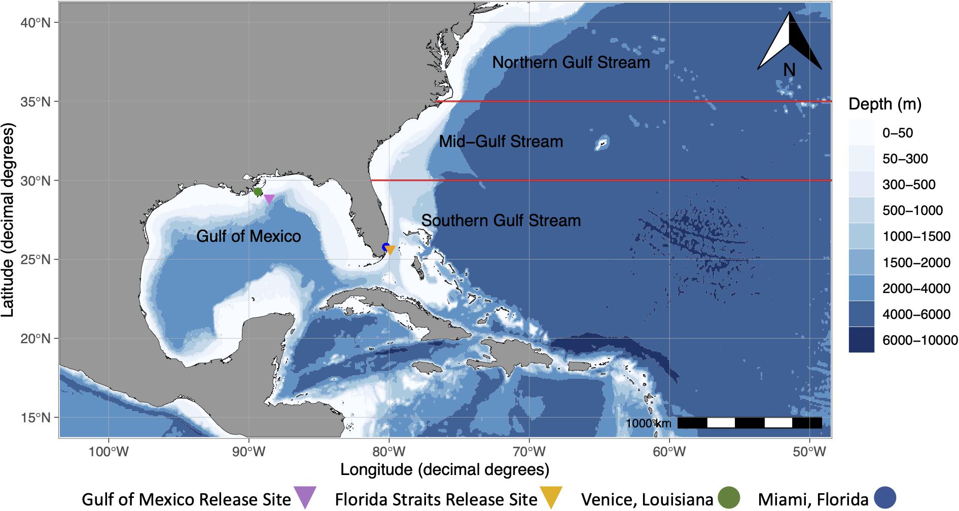
Figure 1. Map showing Venice, Louisiana, Miami, Florida, and generalized release sites for mahi-mahi (Coryphaena hippurus) in the Gulf of Mexico and the Florida Straits. Additionally, four migratory regions (Gulf of Mexico, Southern Gulf Stream, Mid-Gulf Stream, and Northern Gulf Stream), which were determined visually from geolocation tracks and represent four different geographic regions that tagged mahi-mahi inhabited in our study, are shown. The Gulf Stream, a western-boundary current, flows northward from the Florida Straits. The Mid-Atlantic Bight region describes the area originating at the Northern Gulf Stream region north to Massachusetts.
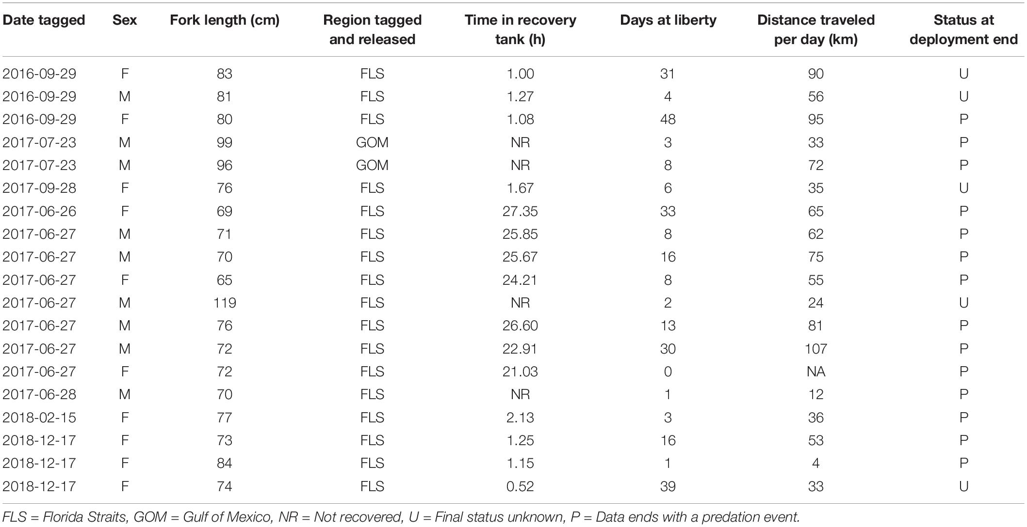
Table 1. Morphometric, release, and migration data from 19 mahi-mahi (Coryphaena hippurus) tagged with pop-up satellite archival tags.
Due to the sensitivity of mahi-mahi to angling and handling we used an onboard recovery tank (Stieglitz et al., 2017) to allow tagged fish to recover without the threat of predation. In most cases, tagging took place on fishing vessels equipped with a small (1,250 L) or large (5,000 L) recovery tank, although four fish were released immediately following tagging when either the size of the vessel did not permit a recovery tank or time constraints did not allow for recovery. Where recovery tanks were used, fish were introduced to the recovery tank immediately following tagging. Following the recovery period, mahi-mahi were again herded into the sling and released boat-side. Where we were unable to use a recovery tank, tagged mahi-mahi were released boat side from the sling immediately following tagging.
The large recovery tank enabled longer recovery times than the small recovery tank. Mahi-mahi were recovered (mean recovery time for small tank = 1 h 15 min ± 28 min, mean recovery time for large tank = 24 h 48 min ± 2 h 14 min) and released in close proximity to where they were captured. The small recovery tank was oxygenated and was constantly flushed with flow-through seawater. The larger recovery tank was oxygenated and was monitored every 30 min for temperature and salinity (WTW 3310 meter connected to a TetraCon 325 probe, Xylem Analytics, Germany), dissolved oxygen (ProODO optical probe, YSI, Inc., Yellow Springs, OH, United States), pH (Hach H160 meter, Loveland, CO, United States, attached to a Radiometer PHM201 electrode, Copenhagen, Denmark), and ammonia (a micromodified colorimetric assay with indophenol blue) and was maintained on an alternating schedule of 4 h static followed by 1 h of flushing with surface water (mean values: temperature = 29.5°C, pH 8.05, dissolved oxygen = 10.4 mgL–1, salinity = 36.5 ppt, ammonia = 19.97 μmolL–1).
Data Analysis
All analyses were conducted using R software v4.0.3 (R Foundation for Statistical Computing, 2020) with the package tidyverse 1.3.0 (Wickham, 2017), for data management and graphics.
Detection of in situ Spawning Events: Classification Algorithms, Cross-Validation, and Model Assessment
In order to predict probabilities of spawning events in wild mahi-mahi, we used known spawning events observed in wild-caught mahi-mahi in the University of Miami Experimental Hatchery (the controlled environment) in combination with summarized acceleration data to build sex-specific predictive spawning models. We applied a model-averaging (or ensemble modeling) approach by combing predictions from Boosted Regression Trees (BRT; Elith et al., 2008; R package gbm 2.1.8, Greenwell et al., 2018) and Random Forest (RF; Breiman, 2001; R package randomForest 4.6.14, Liaw and Wiener, 2002) models.
The prediction of spawning events in the wild from transmitted acceleration data is entirely novel; however, there were two challenges with these predictions. First, the data were highly imbalanced between the spawning events (the minority class) and non-spawning events (the majority class). Second, the dataset from captive fish was derived from a controlled environment and then used in models to predict spawning events in wild fish, in situ. Thus, robustly evaluating model performance was crucial (He and Garcia, 2009). For each classification algorithm (BRT and RF) and sex, we conducted a leave-one-out cross-validation (LOOCV). For each iteration of the LOOCV we randomly selected 70% of both the spawning events and non-spawning events for the training set and kept the remaining 30% of the spawning and non-spawning events for the validation set. We further applied four treatments to the training set (i.e., the 70% of the captive mahi-mahi data randomly selected) to compensate for the imbalanced nature of the dataset: (1) raw: 70% of the data was randomly selected and used to train the submodel; (2) downsampling: the majority class (non-spawning events) was downsampled by 50%; (3) oversampling: the minority class (spawning events) was randomly oversampled by 150%; and (4) synthetic minority over-sampling technique (SMOTE): a 1:3 spawning:non-spawning ratio was generated with the SMOTE method (Chawla et al., 2002, R package DMwR 0.4.1, Torgo, 2016). This ensured sufficient spawning events were selected to train the submodel in each iteration of the cross validation. No treatment was applied to the 30% of the data used for validating the submodels in each iteration.
The classification submodel was then trained to predict spawning events observed in captive mahi-mahi. The BRT submodel was trained with the time fish spent in a low-activity state and the count of acceleration events during the spawning events, the changes in these summarized movement parameters three, two, and one time step(s) before spawning events, and the changes in summarized movement parameters one and two time step(s) after spawning events. Additionally, the anomaly of time spent in a low-activity state compared to the mean for each fish, the anomaly of acceleration events compared to the mean for each fish, the ratio of time in a low-activity state to acceleration events, the ratio of acceleration events to time in a low-activity state, the time since sunset at the time of spawning, and the moon illumination at the time of spawning were included in the BRT submodel.
The number of trees was fixed to 10,000 to allow systematic convergence and, given the high number of variables used as predictors, the interaction depth was set to one. To allow higher variability among algorithms, the RF models were trained with fewer predictors (the time in a low-activity state and the count of acceleration events during the spawning events, the change in percent time in a low-activity state and counts of acceleration events one time step before the spawning events, the change in percent time in a low-activity state and counts of acceleration events one and two time step(s) after the spawning event, the time since sunset and the moon illumination). At the end of each iteration of the LOOCV, the trained submodel was used to predict the validation subset. Then, receiver operating characteristic (ROC) curves (Fawcett, 2006; R package pROC 1.16.2, Robin et al., 2011) were computed and used to objectively estimate the probability threshold above which events should be considered as true (i.e., predicted spawning events) and the standard performance metrics were computed (area under the curve, accuracy (modified for imbalanced datasets), specificity, recall, precision, and F1-score). The submodel was finally used to predict spawning events in the in situ dataset, and the submodel’s performance metrics and predictions were assessed.
The goal of this research was to detect the most-likely spawning events in situ without the necessity of recapturing PSATs. Therefore, once all submodels were trained and used to predict the spawning events in wild fish for each classification method and sex, we selected the iteration that maximized the recall, the proportion of true positives (i.e., the most-likely spawning events) detected by the models. The oversampling + downsampling treatment of the training set had a mean recall of 0.85. We then computed the predicted probability of spawning for each fish for each 2-h time period in the wild as the weighted mean of the predicted probabilities from each iteration, using the recall of the submodels as the weighting function. This approach enabled us to give more weight to the predictions of the submodels that had the highest recall.
Model Averaging to Detect in situ Spawning Events in Male Mahi-Mahi
For male mahi-mahi, there was a strong correlation in the predicted probabilities of spawning from both BRT and RF models (F1–903 = 892.5, R2adj = 0.497, p < 2.2 × 10⁻¹⁶; Figure 2A). Here, the model-averaged spawning probabilities range from min = 0 to max = 0.66, with a mean 0.14, a median of 0.056 and a quantile 75% of 0.14.
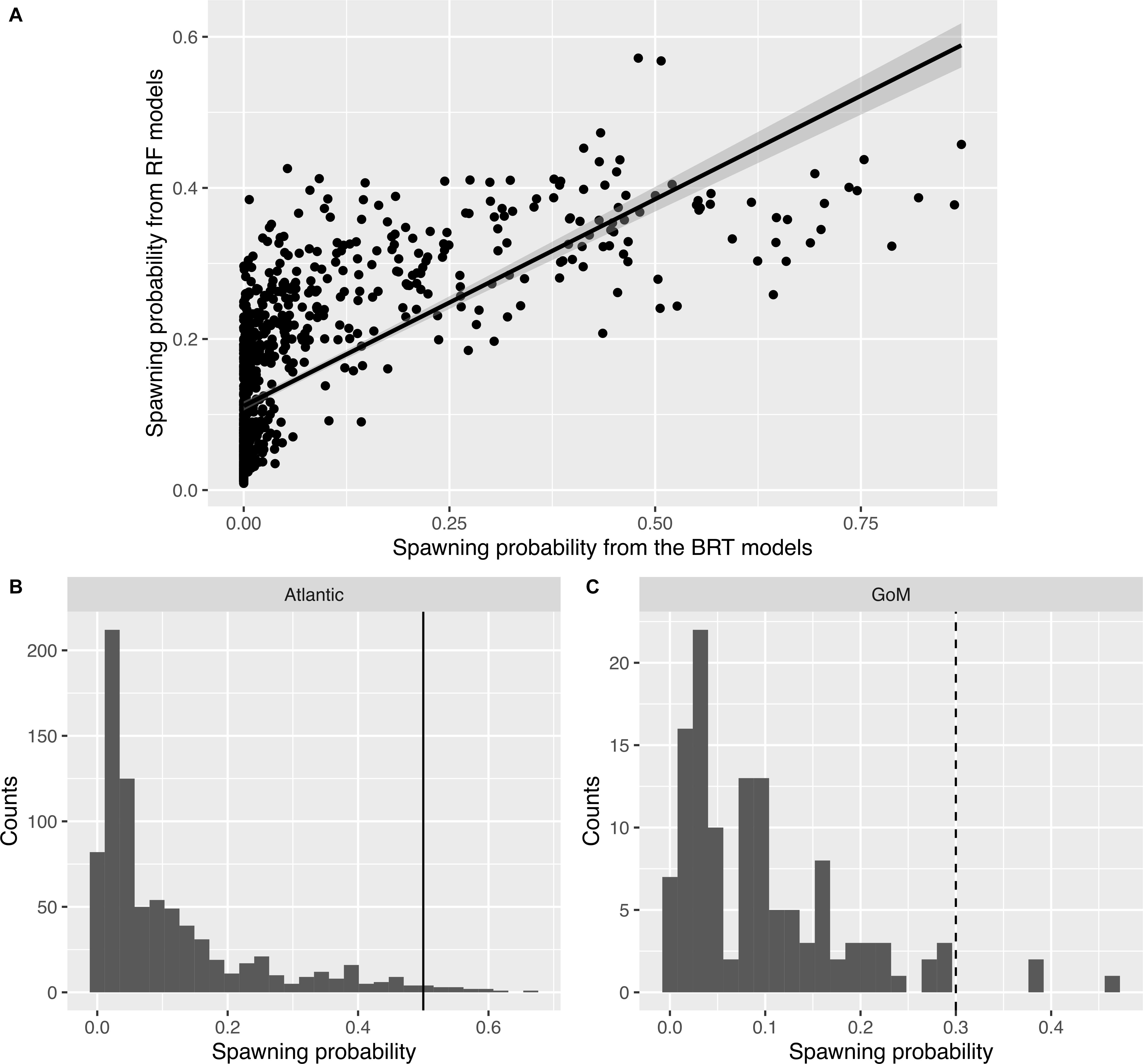
Figure 2. Distributions of predicted spawning probabilities in male mahi-mahi (Coryphaena hippurus). (A) Relationship between the spawning probabilities predicted from the Boosted Regression Tree models (x-axis) and from the Random Forest models (y-axis). (B) Histograms of spawning probability and thresholds used to define predicted spawning events in situ for the Atlantic region (plain line: th = 0.5). (C) Same as panel (B) for the Gulf of Mexico (dashed line: th = 0.3).
The threshold to assign spawning events was set to 0.5 for males in the Atlantic region (Figure 2B). With this approach, events that had an average probability of over 50% from both methods were considered likely spawning events. In the Gulf of Mexico, where only two male fish were tagged, a lower threshold was selected as no event reached a 50% model-averaged probability. We thus chose a threshold of 30% for males in the Gulf of Mexico as that approach selected the few events with the highest probabilities that appear separated from the core of the distribution (Figure 2C), while still remaining higher than the threshold from the submodels (0.023 for BRT and 0.16 for RF).
Model Averaging to Detect in situ Spawning Events in Female Mahi-Mahi
For wild female mahi-mahi, discrepancies in the high probabilities of spawning events from the two classification algorithms (RF and BRT, F1–1780 = 169.8, R2adj = 0.09, p < 2.2 × 10⁻¹⁶; Figure 3A) led to relatively low probabilities of spawning events after model averaging (spawning probabilities ranging from min = 0 to max = 0.32, with a mean of 0.035, a median of 0.023 and a quantile 75% of 0.046).
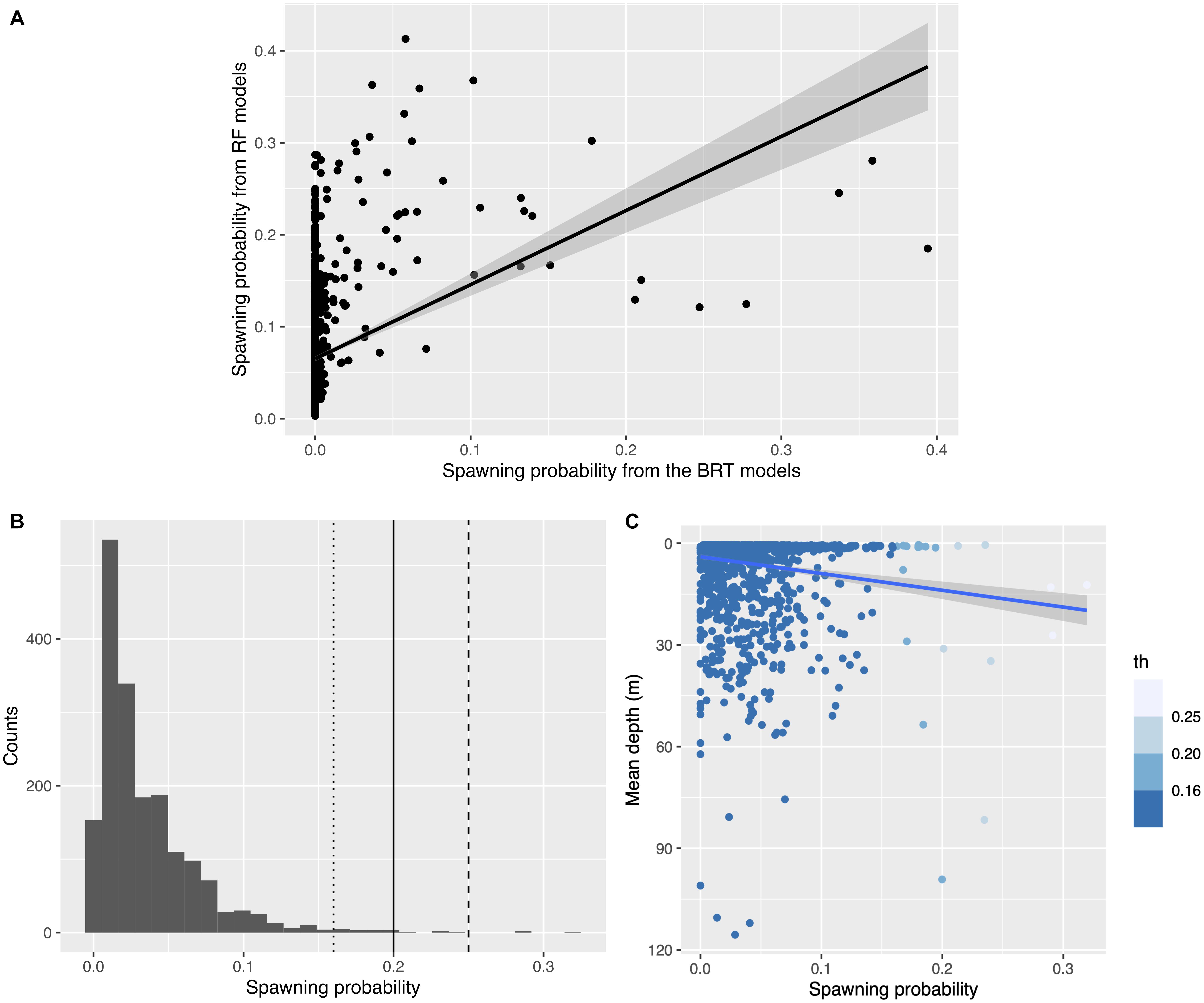
Figure 3. Distributions of the predicted spawning probabilities in wild female mahi-mahi (Coryphaena hippurus). (A) Relationship between the spawning probabilities predicted from the Boosted Regression Tree models (x-axis) and from the Random Forest models (y-axis). (B) The three thresholds of spawning probability used to define predicted spawning events in female mahi-mahi in situ using our model averaging approach (dotted line: th = 0.16, plain line: th = 0.2, dashed line: th = 0.25). (C) Relationship between the mean depth of the predicted in situ spawning probability, colored by the three thresholds selected. The relationship is weak but significant (R2adj = 0.021, F = 40.1, p = 3.04e-10).
To define a threshold above which events would be considered spawning events, we tested three thresholds (th = 0.25, 0.2, and 0.161) and estimated the sensitivity of the results. The highest threshold was chosen to correspond to a spawning probability over 50% in each predictive model, the 0.2 threshold corresponds to a spawning probability over 45% in each model, and the 0.16 threshold represents a spawning probability over 40% in each model (Figure 3B). Each of these thresholds is above the mean cut-point generated by the ROC curve for each method (0.015 for BRT and 0.14 for RF). This allowed a focus on the most-likely events among the predicted spawns, an approach which decreased the rate of false positives. Decreasing the threshold from 0.25 to 0.2 and then to 0.16 increased the number of predicted spawning events to 3, 8, and 21, respectively.
The choice of threshold had little effect on the predicted spawning mean depth of wild female mahi-mahi. With th = 0.25, the mean depth for non-spawning events was 7.95 and 17.5 m for predicted spawning events; at th = 0.2, the mean depth for non-spawning events was 7.77 and was 25.1 m for spawning events; and for th = 0.16, the predicted mean non-spawning depth was 7.67 and 18.7 m for predicted spawning events. Even with the variability among thresholds, each threshold demonstrated a systematically deeper mean depth for predicted spawning events compared to predicted non-spawning events. The relatively deep predicted spawning depth with th = 0.2 is due to two events of high spawning probabilities that occurred between 80 and 100 m depth (Figure 3C). Our data show that mahi-mahi rarely make such deep excursions, making it unlikely that spawning occurred at those depths. Omitting these two predicted events classified with th = 0.2 drives the predicting non-spawning depth to 7.89 m and the predicted spawning depth to 17.1 m which is highly comparable to the other thresholds. This suggests that over this range of th values, the threshold has a limited influence on the predicted spawning depth. In each case, the mean predicted spawning depth was significatively deeper, or approached a significant difference, than the mean nighttime depth (Wilcoxon test, th = 0.25, W = 4812, p = 0.01; th = 0.2, W = 10,543, p = 0.012; th = 0.16, W = 22,198, p = 0.079). For our analysis, we chose the intermediate threshold th = 0.2 because it corresponded to the upper tail of the probability distribution and enabled a reduction in the risk of false positives while not discarding likely spawning events (Figures 3B,C).
Analysis of Activity, Depth, Temperature, and Light Data
Depth and light level data were examined to determine when PSATs detached from mahi-mahi or when predation events occurred. Predation events were identified by continued changes in depth and temperature with concomitant cessation of light data, together indicating the tag had been swallowed. Premature PSAT detachment was identified when no changes in depth were evident for extended periods, indicating that the tag was floating at the surface. TrackIt, a state-space Kalman filter model was used to estimate twice-daily positions for each mahi-mahi using transmitted light data collected at sunrise and sunset and SST measured by the tag at sunrise and sunset and by National Oceanic and Atmospheric Administration satellite data (Lam et al., 2010). To refine tracks from two mahi-mahi that had estimated positions that fell on land, a proprietary software from the tag manufacturer was used for alternate location estimates using the transmitted light-level data (WC-GPE v.201805, Wildlife Computers). Additionally, results from the WC-GPE software were used to calculate minimum travel for each fish’s deployment period as well as the daily minimum travel distance.
To consider whether possible stress effects from tagging and handling were biasing temperature, depth, or activity results we sequentially left out the initial 1, 2, 3, 5, and 7 days of data post-release, and examined model consistency. Each of the most parsimonious models for depth, temperature, and high activity periods were assessed with the full dataset as well as with the various timepoints withheld from the data.
Linear models to predict temperature, depth, and activity used individual fish as a random effect (R package lme4 1.1, Bates et al., 2015). Assignment of diel period (e.g., day or night) for linear models was assigned using each fish’s estimated daily locations and local sunrise and sunset for those locations (R package RchivalTag, Bauer, 2020). Akaike’s Information Criterion (AIC; Akaike, 1973; Burnham and Anderson, 2002) was used to discriminate among competing formulations when multiple linear models were considered. P-values for explanatory variables were calculated using an analysis of variance to compare a model with only an intercept and the random effects to models with each individual explanatory variable as well as the random effects (α = 0.05). Where noted, errors are reported as plus or minus one standard deviation.
A linear model was used to assess the role of PSAT-derived SST, the fraction of moon illumination, and whether it was day or night in predicting depths of wild fish. A second linear model was used to predict temperatures that wild fish inhabited using the current location of each fish and day or night period. PSAT-derived SST was calculated daily for each individual fish from the mean temperature measured by the tag every time that the fish was in the top 2 m of the water column. Migratory regions were determined visually from geolocation tracks and represent four different geographic regions that tagged mahi-mahi inhabited in our study. Regions were designated as the Gulf of Mexico (>81°W and >25°N), the southern Gulf Stream (<30°N), mid-Gulf Stream (30°N–35°N), or northern Gulf Stream (>35°N; Figure 1).
Acceleration events frequently exceeded the maximum value within a 2-h period and maximum values were represented more frequently than other counts. Therefore, we defined an activity index where occurrences of the maximum number of acceleration events were considered a period of high activity, while all other counts of acceleration events were considered periods of reduced activity. We used mixed effect logistic regression models to examine the role of PSAT-derived SST, lunar phase, and day or night period in predicting periods of high activity in wild fish. Additionally, we used the same methodology to examine the role of lunar phase and day and night period in captive-tagged fish.
Results
Predicted Spawning and Migrations
Pop-up satellite archival tag deployments on wild mahi-mahi collected 270 days of data from 19 fish at liberty for up to 48-days (Table 1). No major shifts in parameters were observed in models that dropped the first 1, 2, 3, 5, and 7 days of data to examine potential stress effects and therefore the full dataset was used for all models (Figure 4 and Table 2).
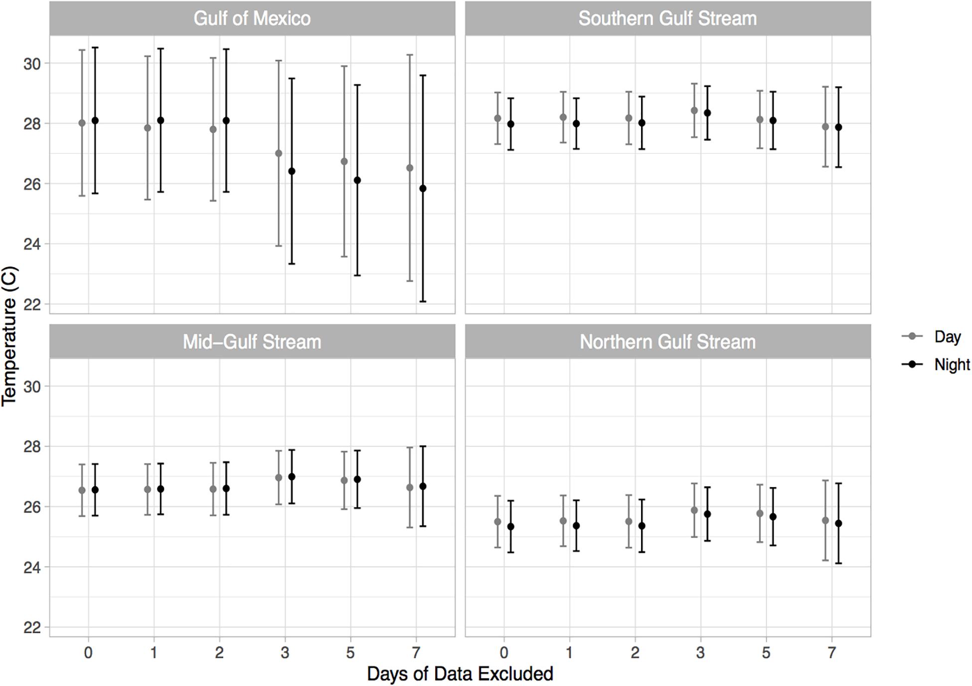
Figure 4. Estimated thermal preference of mahi-mahi (Coryphaena hippurus) from linear mixed effect models predicting temperature from geographical region and diel period. Results from the full model as well as models leaving out the first 1, 2, 3, 5, and 7 days of data are shown. Model runs were performed with an increasingly greater number of days of data withheld to assess whether any altered behaviors that might occur after release were influencing the results.
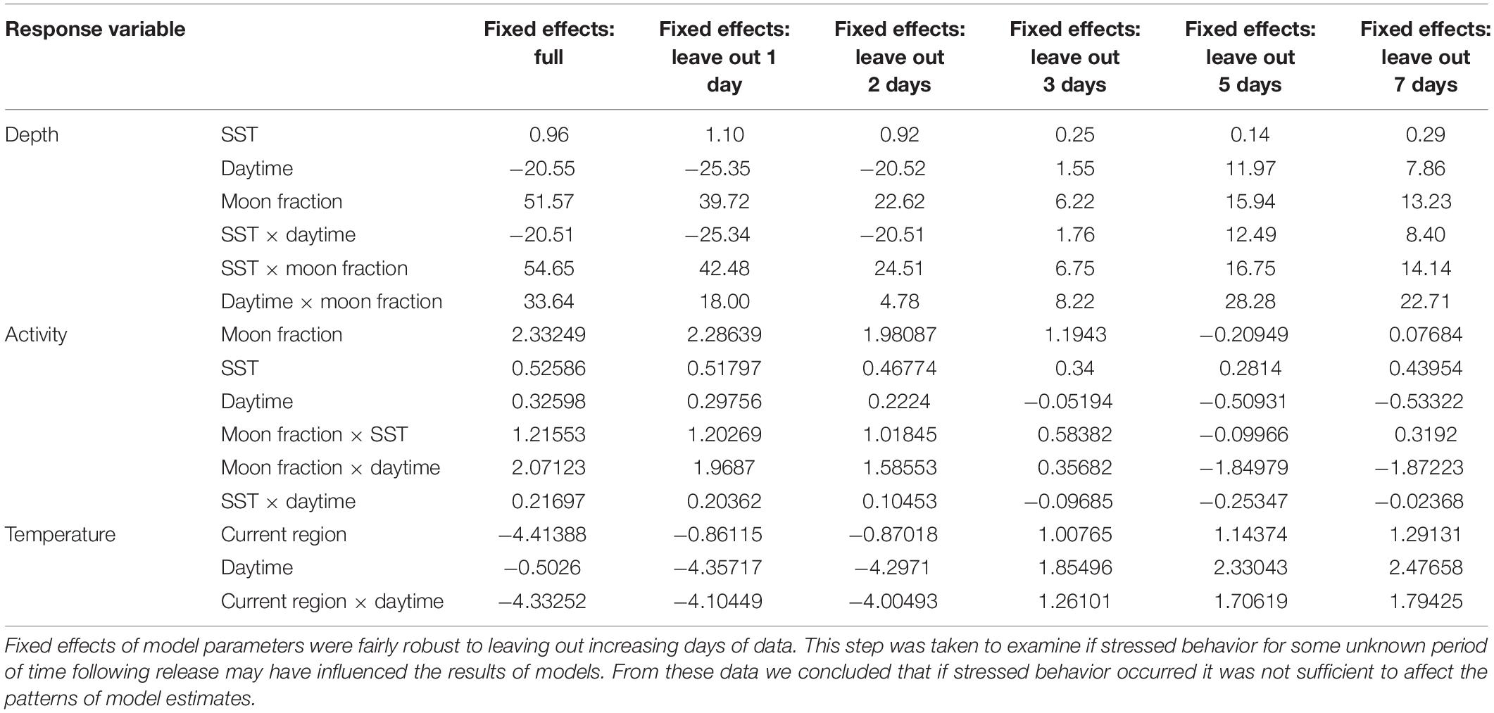
Table 2. Fixed effects of full depth, activity, and temperature models for wild mahi-mahi (Coryphaena hippurus) tagged with pop-up satellite archival tags, and iterations leaving out the first 1, 2, 3, 5, and 7 days of data.
In wild mahi-mahi, predicted spawning occurred at night an average of 7.4 and 6.4 h after local sunset in females and males, respectively (range of 3.0–10.8 h post-sunset in females and 5.2–8.9 h in males). Seven out of nine tagged males and 2 out of 10 female mahi-mahi spawned repeatedly. For all fish that were predicted to have spawned more than once, the period between spawns was highly variable and was between 2 h and 21 days (mean = 2.7 days) in males and between 22 h and 12.5 days (mean = 7.2 days) in females. Overall, predicted spawning occurred most frequently around the new moon phase in the lunar cycle in both males and females.
Mahi-mahi spawning events were predicted at a mean depth of 17.0 ± 19.1 m. In the Atlantic, the probability of spawning increased with depth and spawning events with the highest probabilities occurred at significantly greater depths than the nighttime depths occupied by non-spawning fish (Figure 5). For females, the mean predicted spawning depth (25.1 m) was over 17 m deeper than the mean non-spawning nighttime depth (7.77 m; Wilcoxon, W = 10,543, p = 0.01; Figure 5). For males, the mean expected spawning depth was 13.2 m while their mean expected non-spawning nighttime depth was 5.54 m (Wilcoxon, W = 49, p = 0.03; Figure 5). In contrast, the two male mahi-mahi tagged in the Gulf of Mexico tended to be deeper during predicted non-spawning periods and moved shallower for spawning (mean predicted spawning depth was 14.3 m and mean predicted non-spawning nighttime depth was 32.5 m; Wilcoxon, W = 8636.5, p = 0.003; Figure 5). Although the directional change between expected spawning and non-spawning periods was reversed between males in the Atlantic and Gulf of Mexico, the predicted spawning depths and temperatures were similar between regions.
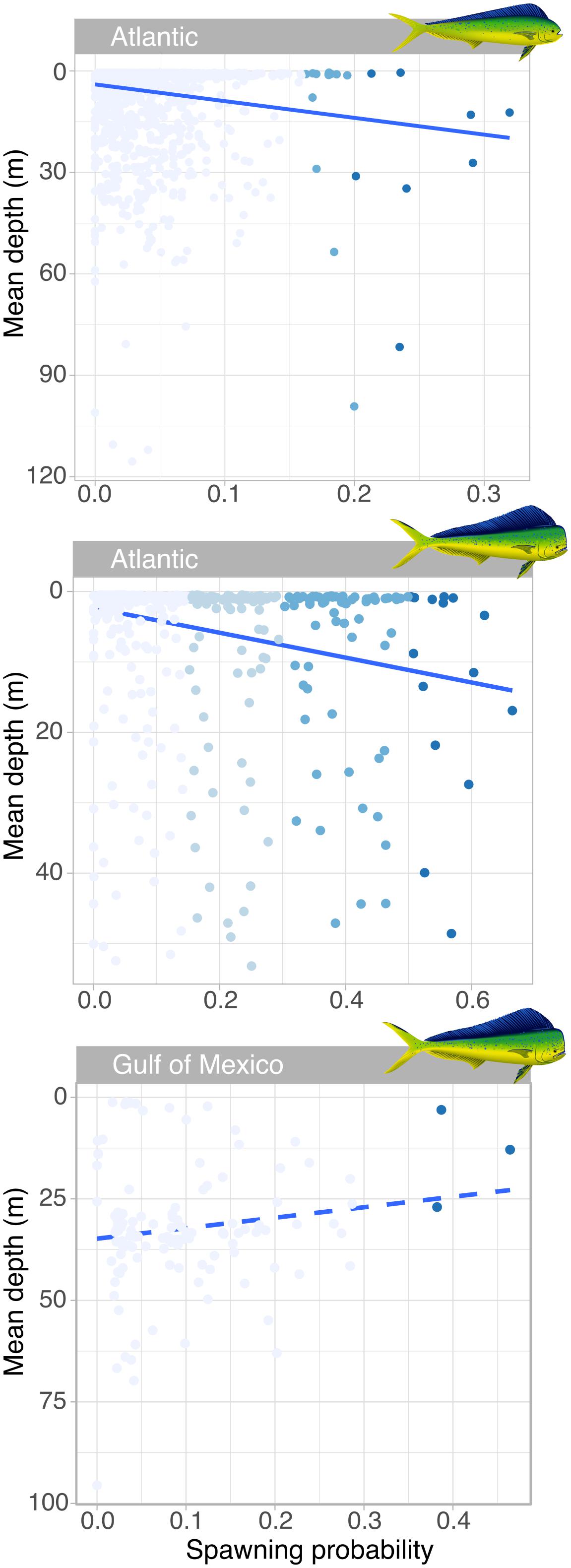
Figure 5. Relationship between probability of spawning events in the wild and mean depth in female (upper panel) and male (lower panels) mahi-mahi (Coryphaena hippurus). Coloration of points show the different thresholds considered for determining predicted spawning events, with the darkest blue dots representing events with the highest threshold and greatest probability of spawning for each sex and region. In the Atlantic, the linear relationship between the spawning probability and mean depth is significant for males (R2adj = 0.057, t = 49.5, p = 4.22 × 10⁻¹²; plain line) and females and shows increased depth at spawning (R2adj = 0.022, t = 40.1, p = 3.05 × 10–1012; plain line), while males in the Gulf of Mexico moved shallower for predicted spawning (R2adj = 0.013, t = 2.62, p = 0.10; dashed line).
Light data collected by PSATs revealed that mahi-mahi tagged in the warmest months (June and September) off the Florida Atlantic coast migrated northwards with the Gulf Stream current traveling a daily minimum distance of up to 107 km d–1 (Table 1). As they reached the Mid-Atlantic Bight and cooler waters, trajectories became more oriented to the east and then the southeast (Figures 1, 6). The majority of predicted spawning events were concentrated off Florida’s Atlantic coast in June, July, and September; however, this also overlaps with the region and time of year that the vast majority of mahi-mahi were at liberty. Nevertheless, mahi-mahi tagged >30 days were predicted to have >60% of their spawning events take place off Florida’s Atlantic coast region despite spending the majority of their time further north. Overall, temperatures between 27.5 and 30°C encompassed all but one predicted spawning event. Three mahi-mahi tagged off Florida’s Atlantic coast in December remained within that region for the duration of tagging and were not predicted to have spawned over a combined 56 days at liberty. The sole predicted spawning event to occur at cooler temperatures took place at the end of February off Florida’s Atlantic coast at 24°C, suggesting that some limited spawning may occur in late winter in the sub-tropics (Figure 6).
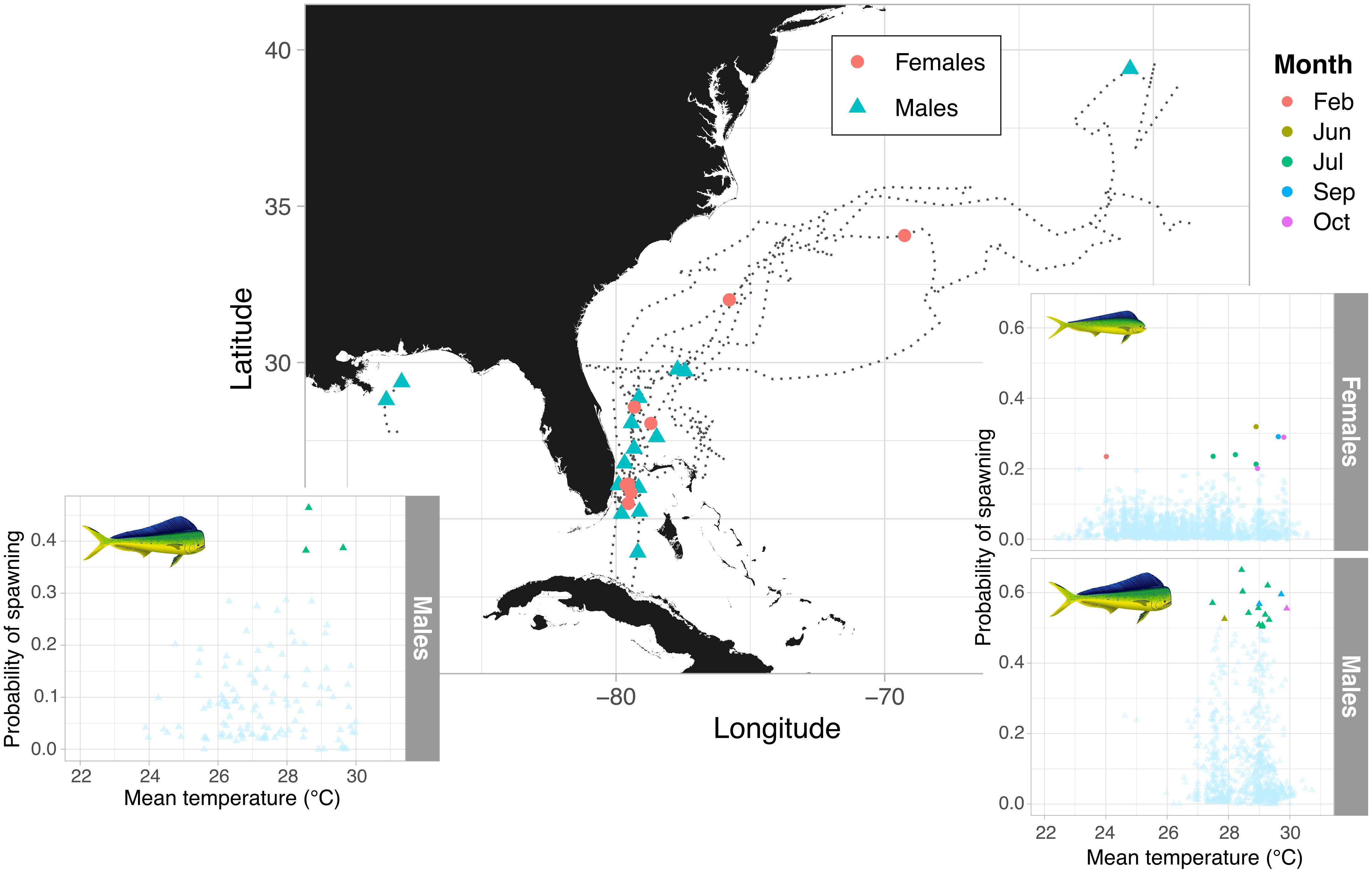
Figure 6. Spatial distribution of predicted spawning events and individual migratory patterns in female and male mahi-mahi (Coryphaena hippurus) tagged with accelerometer equipped PSATs. The distribution of spawning probabilities with temperature and month is shown for the Gulf of Mexico and Atlantic in the subpanels, with the multi-colored points showing the predicted spawning events.
Relative Activity, Depth, and Temperature of Wild Mahi-Mahi
Summarized acceleration data, in addition to predicting spawning, was also used to classify periods of high and reduced activity. SST, diel period (i.e., daytime or nighttime), and lunar phase significantly affected mahi-mahi activity and depth distributions (Table 3). Across their migrations, mahi-mahi occupied temperatures from 17 to 32°C but spent 95% of their time in water between 25 and 29°C and displayed little variation in median temperature between distinct migratory regions (regional median temperature range = 27.0–27.9°C, overall median temperature = 27.5°C, Figures 7A, 8). To maintain this narrow thermal window, mahi-mahi used behavioral thermoregulation and moved deeper in the water column as SST increased (Figures 8, 9B,C and Table 3). Mahi-mahi were generally surface oriented but occasionally descended as deep as 250 m (Figure 7B), and in regions with the warmest SSTs mahi-mahi were consistently deeper during daytime hours than in regions with cooler SSTs (Figure 8). When the effect of SST was held constant, mahi-mahi were consistently deeper and made more frequent excursions to depth at night than during daylight hours. However, our data show that below 25°C SST fish remained very close to the surface regardless of diel period. Additionally, at nighttime mahi-mahi were closest to the surface during the full moon and moved deeper as moon illumination waned (Figures 9A,C). Activity generally declined with increasing SST and was moderate at ∼27°C (Figures 10B,C and Table 3). Above ∼27°C SST, nighttime activity increased with increasing lunar illumination, while conversely, below that temperature the opposite trend occurred (Figures 10A,C). Similarly, our wild-caught captive-tagged mahi-mahi, held at 27°C and used to build spawning models, increased activity as the full moon approached (Figure 11 and Table 3).
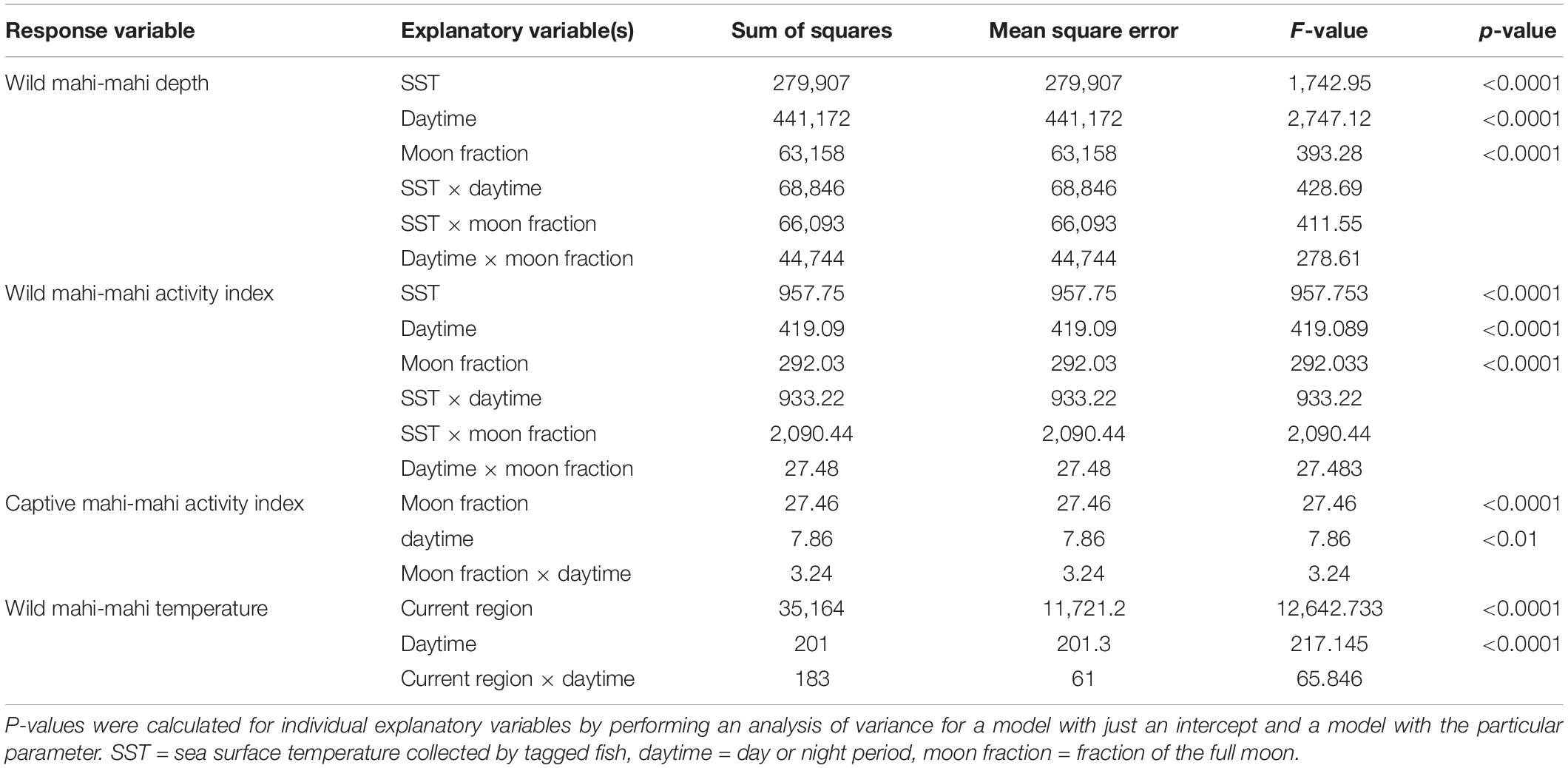
Table 3. Parameters of best linear mixed effect models fitted to depth, summarized acceleration activity index, and temperature data collected from 19 wild mahi-mahi (Coryphaena hippurus) released in the Florida Straits and the Gulf of Mexico and five captive mahi-mahi tagged with pop-up satellite archival tags.
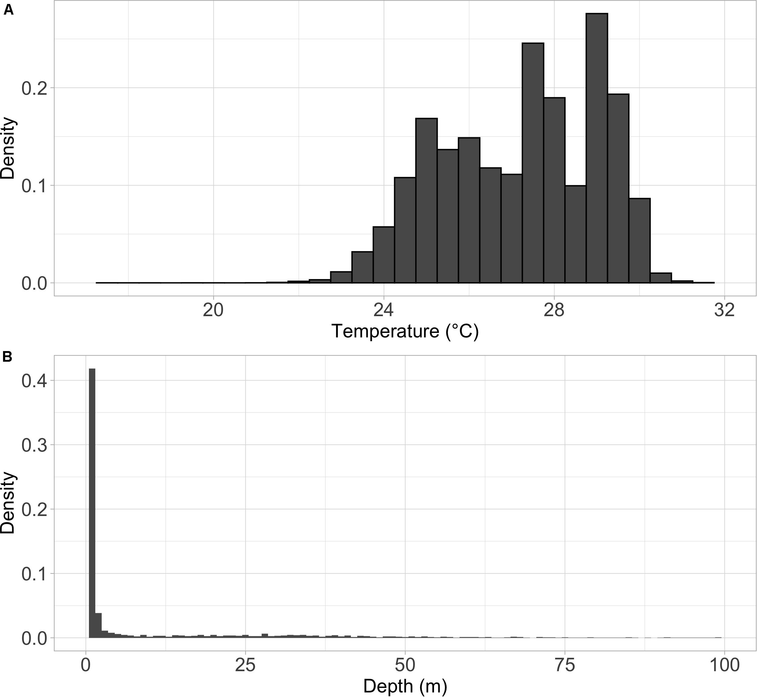
Figure 7. Density histogram of the (A) temperature and (B) depth distributions for mahi-mahi (Coryphaena hippurus) tagged with pop-up satellite archival tags and released in the Florida Straits and the Gulf of Mexico. Depth histogram shows only the top 100 m of the water column. Mahi-mahi spent the vast majority of their time in surface waters but periodically explored depths as deep as 250 m and spent 95% of their time in waters from 25 to 29°C.
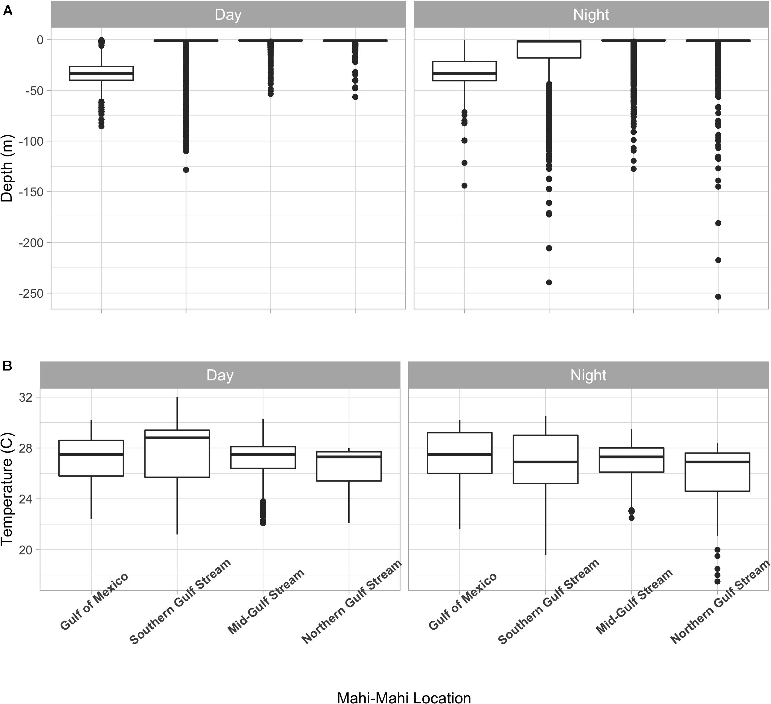
Figure 8. Depth (A) and temperature (B) distributions of tagged mahi-mahi (Coryphaena hippurus) by region. Median values are represented by the horizontal black lines, the white box represents the interquartile range, the black vertical lines represent the smallest and largest values within 1.5 times the interquartile range above the 75th percentile or below the 25th percentile, and the black circles represent values that fall outside of that range.
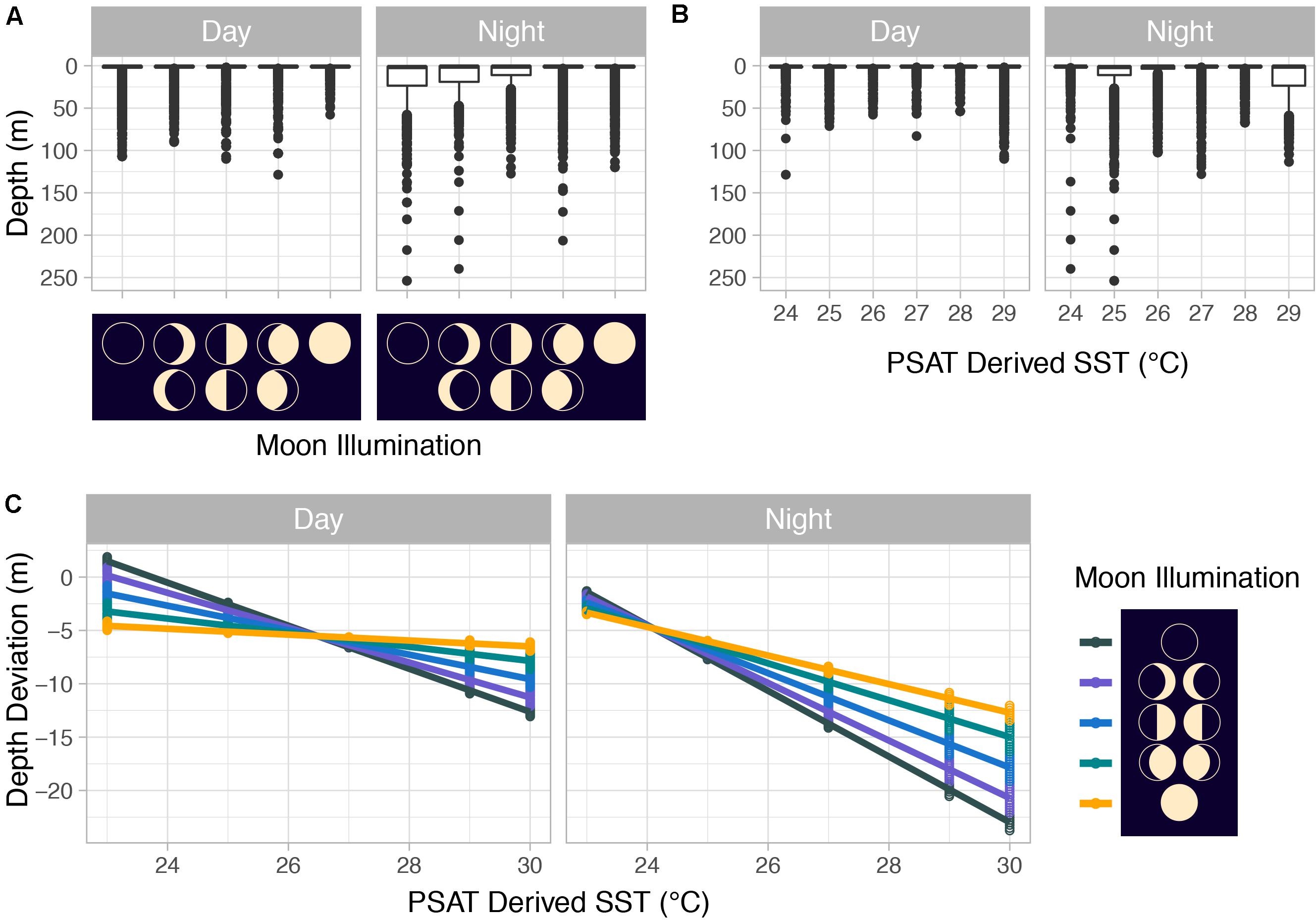
Figure 9. (A) Mahi-mahi (Coryphaena hippurus) depth distributions by moon phase and by (B) PSAT-derived SST as well as (C) depth distributions from linear mixed effect models predicting depth from PSAT-derived SST, moon illumination, and diel period. For panels (A,B), median values are represented by horizontal black lines, white boxes represent the interquartile range, black vertical lines represent the smallest and largest values within 1.5 times the interquartile range above the 75th or below the 25th percentile, and black circles represent values that fall outside of that range.
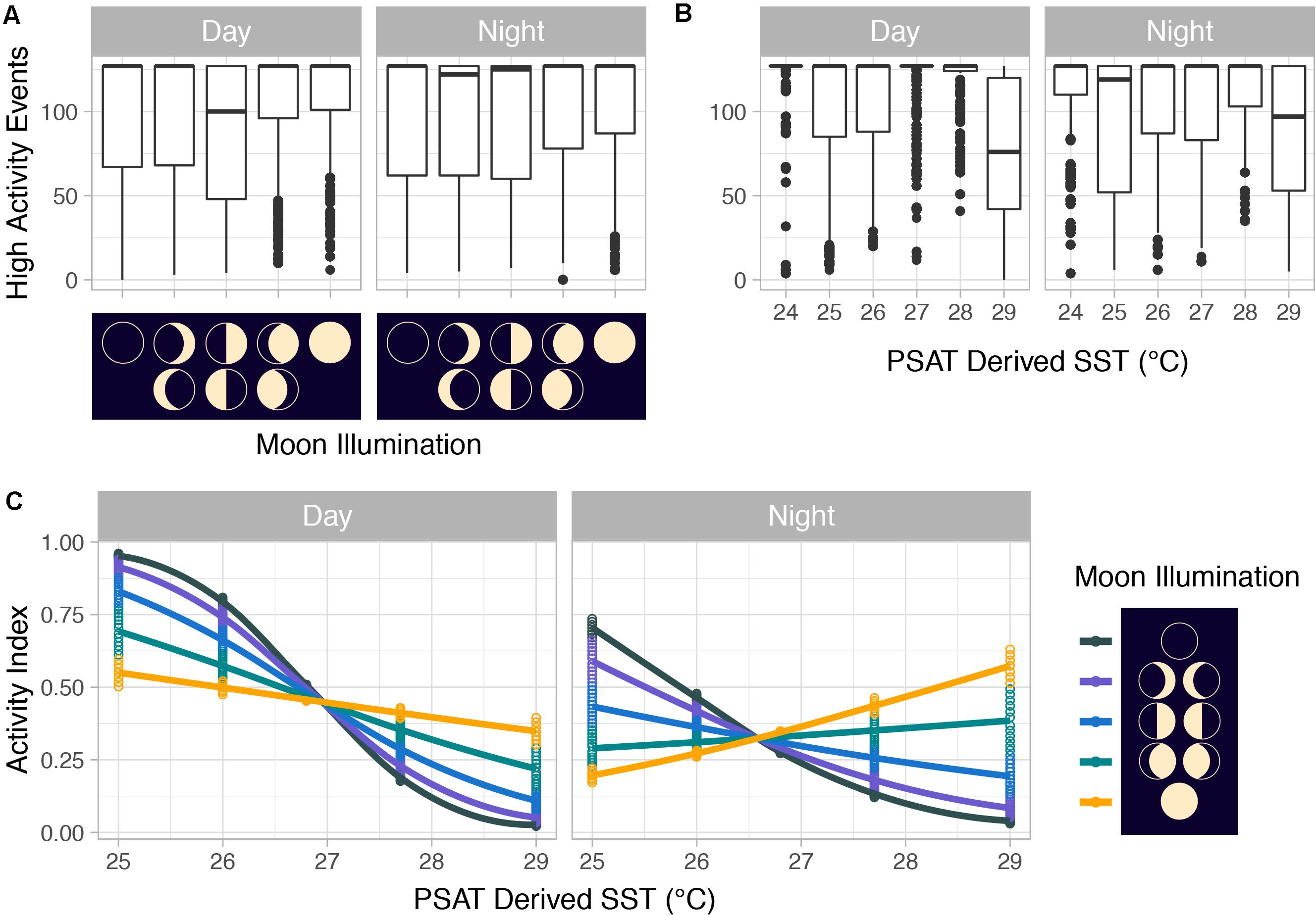
Figure 10. (A) Counts of mahi-mahi (Coryphaena hippurus) high-activity events with moon phase and (B) with PSAT-derived SST as well as (C) activity distributions from mixed effect logistic regression models predicting activity from PSAT-derived SST, moon illumination, and diel period for wild mahi-mahi. For panels (A,B), median values are represented by horizontal black lines, white boxes represent the interquartile range, black vertical lines represent the smallest and largest values within 1.5 times the interquartile range above the 75th or below the 25th percentile, and black circles represent values that fall outside of that range.
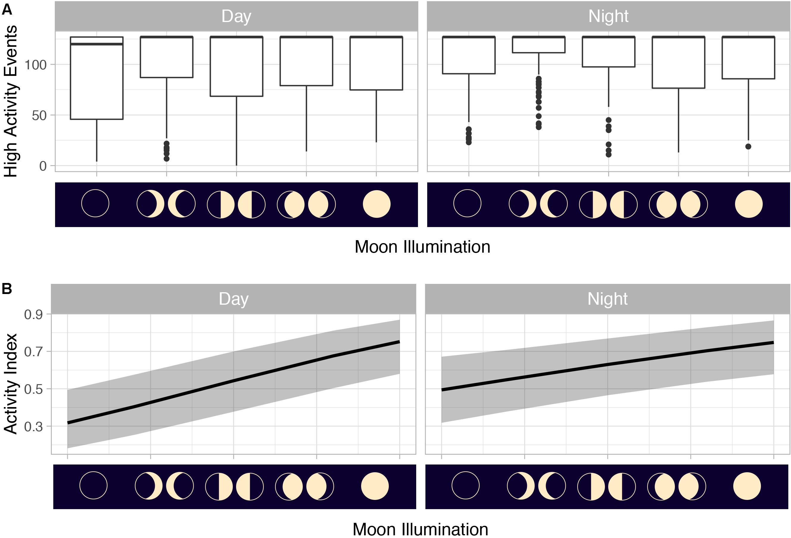
Figure 11. (A) Counts of mahi-mahi (Coryphaena hippurus) high-activity events (>0.65798 g) by moon phase and (B) activity distributions from mixed effect logistic regression models predicting activity from moon illumination and diel period in captive mahi-mahi. For panel (A) median values are represented by the horizontal black lines, the white box represents the interquartile range, the black vertical lines represent the smallest and largest values within 1.5 times the interquartile range above the 75th percentile or below the 25th percentile, and the black circles represent values that fall outside of that range. For panel (B) solid lines represent model predictions and shaded gray area represents the 95% confidence interval.
Discussion
Tags in the present study were programmed to pop-up at 96 days; however, retention ranged from less than 1 day up to 48 days. This is a relatively short tag-retention period compared to other pelagic species tagged with PSATs (Lam et al., 2016), but longer than or similar to other studies on mahi-mahi (Merten et al., 2014, 2016; Lin et al., 2019). It is not always possible to discern why PSAT deployments end prematurely, but for nearly three-quarters of our mahi-mahi, including our longest tagged, deployments ended in predation (Table 1). Periods of stress from the tagging process or carrying a PSAT have been suggested for pelagic fishes for 2–6 h after release (Brill et al., 1993); however, relatively short tag retention may also be explained by the high annual natural mortality rate in mahi-mahi in the western central Atlantic (97–99.9%) (Oxenford, 1999). To assess the possibility of stressed behavior influencing our results, we elected to drop the first 1, 2, 3, 5, and 7 days of data from our temperature, depth, and activity models. We observed consistency in model parameters across these iterations which suggests that any stress effects present in our tagging data did not influence our results. In support of this conclusion, tagged and untagged mahi-mahi swimming freely in a shared tank show no difference in survival, overall distance traveled, acceleration, mean velocity, maximum velocity, or feeding success (McGuigan et al., 2021). These results demonstrate that our data can be interpreted with confidence.
Our predicted spawning events in wild mahi-mahi are built solely with the PSAT-summarized acceleration data and are the first of their kind. Spawning events were predicted to occur at night, primarily off the Florida Atlantic coast, at temperatures largely between 27.5 and 30°C, at a distinct depth from the mean nighttime depth distribution, and primarily at the new moon. Predicted spatiotemporal spawning habitat was similar for tagged males and females in our study and estimates of spawning depth for the sexes had overlapping confidence intervals. The variation we observed in both the timing and the depth distributions of predicted spawning events between males and females is likely due to local variation in oceanographic conditions and may be a factor of our relatively small sample size. Despite mahi-mahi in the Gulf of Mexico occupying a deeper distribution during non-spawning periods than in the Atlantic, spawning depths were similar between basins. Starting on the second day of development, mahi-mahi embryos have dynamic control over their buoyancy, and become negatively buoyant after exposure to ultraviolet radiation – a mechanism thought to be a protective adaptation to avoid exposure to this stressor (Pasparakis et al., 2019). Spawning at depth has also been shown to be an adaptive strategy to protect teleost embryos from ultraviolet radiation (Huff et al., 2004), suggesting that the basin-independent spawning depth selected by mahi-mahi may protect embryos from exposure before they are able to modulate their buoyancy.
Mahi-mahi in our study demonstrated daily minimum travel distances as high as 107 kmd–1 and migrated in a seasonal clockwise pattern that has been previously observed in mahi-mahi in the western Atlantic (Oxenford, 1999; Merten et al., 2016). Spawning predictions from our data additionally suggest a strong seasonal pattern and support temporal observations of mahi-mahi larvae that also agree with gonad development of adult mahi-mahi in the western central Atlantic (Gibbs and Collette, 1959; Beardsley, 1967; Oxenford, 1999). The majority of predicted spawning events took place in the summer months in the Gulf Stream off Florida’s coast where oceanographic features concentrate warm high-salinity waters in a tightly confined channel, which may be beneficial for spawning. Although our captive mahi-mahi, and thus our captive acceleration data set, did not experience the full range of stimuli (e.g., live prey and predators) that wild tagged fish encountered, captive spawning events were not defined simply by periods of greater acceleration, but by the relative change in acceleration patterns and include sustained periods of slower swimming that were not observed at other times. Thus, wild prey capture or predator avoidance alone, are unlikely to have resulted in false positives of predicted spawning events in wild mahi-mahi. While false-positive predictions among our collective predicted spawning events in wild mahi-mahi are probable, we are confident that as a whole, our predictions provide useful information on likely spatiotemporal spawning habitat for the species. Accurate spawning predictions are critical for estimating the productivity of species and understanding population connectivity (Lowerre-Barbieri et al., 2017). Applied to other species this approach may provide greater insight into spawning frequency and habitat than had previously been described from traditional methods and could aid in the discovery of new spawning grounds.
Activity indices defined from summarized acceleration data provide insight into the potential foraging strategies and baseline activity of mahi-mahi over a range of SSTs and lunar phases. At the coldest SSTs, mahi-mahi were the closest to the surface and the most active at the new moon, a pattern that mirrors the lunar depth distribution of the deep scattering layer, a group of mesopelagic fishes and plankton (Benoit-Bird et al., 2009), which may be prey for mahi-mahi who are known to feed at the surface (Oxenford and Hunte, 1999). In contrast, during the full moon above ∼27°C SST, mahi-mahi were consistently shallower and more active than at lower levels of lunar illumination, which could suggest that in warm waters mahi-mahi capitalize on lunar illumination for feeding closer to the surface at nighttime.
Daytime depth and activity distributions were also affected by lunar phase, which may indicate that nighttime feeding success or failure translates into daytime hunting strategies and depth distributions. In support of this hypothesis, catch-per-unit-effort data from gamefish tournaments show a significant relationship between daytime mahi-mahi catches and lunar phase, with decreased catch rates at the full moon (Lowry et al., 2007). Mahi-mahi do not have vision specialized for low light conditions but despite this limitation they are known to feed at night (Oxenford and Hunte, 1999). The greater depths mahi-mahi occupy at nighttime (Merten et al., 2014, 2016; Lin et al., 2019) may also be a strategy to avoid predators such as billfish that are surface-oriented (Braun et al., 2015), have excellent nighttime vision, and are formidable predators of mahi-mahi. Overall, mahi-mahi were at the greatest depths at nighttime, at the new moon, and with the warmest SSTs, all conditions that our models suggest are most favorable to spawning, indicating that some of their nighttime depth excursions are likely the result of courtship behaviors and spawning. Altogether, our results show how summarized acceleration data greatly expands the ecological information researchers can glean from PSATs, a critical tool to adequately manage highly migratory, and often emblematic, marine species.
Our data show that mahi-mahi tightly maintain a thermal window of 27–28°C during long-distance migrations by modulating their depth and by constraining their latitudinal movements. Similarly, around 27°C we observed intermediate levels of activity, while activity of wild mahi-mahi declined as SSTs increased. Previous short accelerometer deployments on wild mahi-mahi in the East China Sea also showed fewer periods of high activity in warmer seasons (Furukawa et al., 2011). While the current tag data show that mahi-mahi most commonly experience temperatures from 27 to 28°C, tag data alone do not demonstrate the physiological underpinnings that may influence the selection of a narrow thermal zone. However, laboratory-based physiological experiments conducted with mahi-mahi support our findings and add credence to the thermal window hypothesis (Heuer et al., 2021). In tightly controlled physiological experiments, mahi-mahi have their greatest aerobic scope and critical swim speed (Ucrit) at 28°C. Additionally, mahi-mahi demonstrated significant reductions in Ucrit at temperatures above and below 28°C and significant reductions in aerobic scope at temperatures below 28°C (Heuer et al., 2021). Our data from wild mahi-mahi closely mirror these results and suggest that wild mahi-mahi modulate their depth to select a temperature in the wild that maximizes their physiological performance and at which they have moderate activity levels. The top 75 m of the ocean, where mahi-mahi spend the vast majority of their time, warmed more than 0.1°C per decade in the period from 1971 to 2010 as a result of anthropogenic climate change and will continue to increase in temperature (Hoegh-Gulberg et al., 2014). Therefore, when faced with warming seas, mahi-mahi are expected to expand their range toward higher latitudes (Salvadeo et al., 2020), may be deeper and less active in regions where they are already close to their thermal maxima, and could experience spatiotemporal shifts in spawning patterns.
Data Availability Statement
The datasets presented in this study can be found in online repositories. The names of the repository/repositories and accession number(s) can be found below: Gulf of Mexico Research Initiative Information and Data Cooperative (GRIIDC) available at https://data.gulfresearchinititative.org, DOIs: 10.7266/N7ZW1JFW, 10.7266/N7RF5SM6, 10.7266/N7MP51WV, 10.7266/N7H130K5, 10.7266/n7-6c0k-zs94, and 10.7266/TSFAMPZG.
Ethics Statement
The animal study was reviewed and approved by the University of Miami IACUC.
Author Contributions
LSS, JDS, and MG designed the experiment. LSS, RF, and CHL performed and interpreted movement and reproductive modeling. JDS, RHH, DDB, CHL, and CBP contributed biological expertise. LSS, JDS, RHH, GKC, RMH, CP, and MG collected the data. LSS, RF, and MG wrote the manuscript. All authors discussed the results and commented on the manuscript.
Funding
This research was supported by a grant from the Gulf of Mexico Research Initiative [Grant No. SA-1520 to the RECOVER consortium (Relationship of Effects of Cardiac Outcomes in Fish for Validation of Ecological Risk)].
Conflict of Interest
The authors declare that the research was conducted in the absence of any commercial or financial relationships that could be construed as a potential conflict of interest.
Acknowledgments
We thank the students, staff, and volunteers at the University of Miami Experimental Hatchery and the Captains and crews of the R/V Walton Smith, the F/V Miss Britt, and the F/V Triple Threat. MG is a Maytag Professor of Ichthyology.
References
Akaike, H. (1973). 2nd International Symposium on Information Theory. Budapest: Akademiai Kiado, 267–281.
Aranda, G., Abascal, F. J., Varela, J. L., and Medina, A. (2013). Spawning behaviour and post-spawning migration patterns of Atlantic bluefin tuna (Thunnus thynnus) ascertained from satellite archival tags. PLoS One 8:e76445. doi: 10.1371/journal.pone.0076445
Bates, D., Maechler, M., Bolker, B., Walker, S. (2015). Fitting linear mixed-effects models using lme4. J. Stat. Softw. 67, 1–48. doi: 10.18637/jss.v067.i0
Bauer, R. (2020). RchivalTag: Analyzing Archival Tagging Data. R package version 0.1.2. Available online at: https://CRAN.R-project.org/package=RchivalTag (accessed June 1, 2019).
Beardsley, G. L. (1967). Age, growth, and reproduction of the dolphin, Coryphaena hippurus, in the Straits of Florida. Copeia 1967, 441–451. doi: 10.2307/1442132
Benoit-Bird, K. J., Au, W. W., and Wisdoma, D. W. (2009). Nocturnal light and lunar cycle effects on diel migration of micronekton. Limnol. Oceanogr. 54, 1789–1800. doi: 10.4319/lo.2009.54.5.1789
Block, B. A., Dewar, H., Blackwell, S. B., Williams, T. D., Prince, E. D., Farwell, C. J., et al. (2001). Migratory movements, depth preferences, and thermal biology of Atlantic bluefin tuna. Science 293, 1310–1314. doi: 10.1126/science.1061197
Block, B. A., Jonsen, I. D., Jorgensen, S. J., Winship, A. J., Shaffer, S. A., and Bograd, S. J. (2011). Tracking apex marine predator movements in a dynamic ocean. Nature 475, 86–90. doi: 10.1038/nature10082
Braun, C. D., Kaplan, M. B., Horodysky, A. Z., and Llopiz, J. K. (2015). Satellite telemetry reveals physical processes driving billfish behavior. Anim. Biotelemetry 3:2. doi: 10.1186/s40317-014-0020-9
Brill, R. W. (1994). A review of temperature and oxygen tolerance studies of tunas pertinent to fisheries oceanography, movement models and stock assessments. Fish. Oceanogr. 3, 204–216. doi: 10.1111/j.1365-2419.1994.tb00098.x
Brill, R. W. (1996). Selective advantages conferred by the high performance physiology of tunas, billfishes, and dolphin fish. Comp. Biochem. Physiol. Part A Physiol. 113, 3–15. doi: 10.1016/0300-9629(95)02064-0
Brill, R. W., Holts, D., Chang, R., Sullivan, S., Dewar, H., and Carey, F. (1993). Vertical and horizontal movements of striped marlin (Tetrapturus audax) near the Hawaiian Islands, determined by ultrasonic telemetry, with simultaneous measurement of oceanic currents. Mar. Biol. 117, 567–574. doi: 10.1007/bf00349767
Burnham, K. P., and Anderson, D. R. (2002). Model Selection and multimodel Inference: A Practical Information-Theoretic Approach. Berlin: Springer-Verlag, 6–20.
Chawla, N. V., Bowyer, K. W., Hall, L. O., and Kegelmeyer, W. P. (2002). SMOTE: synthetic minority over-sampling technique. J. Artif. Intell. Res. 16, 321–357. doi: 10.1613/jair.953
Cheung, W. W. L., Watson, R., and Pauly, D. (2013). Signature of ocean warming in global fisheries catch. Nature 497, 365–368. doi: 10.1038/nature12156
Elith, J., Leathwick, J. R., and Hastie, T. (2008). A working guide to boosted regression trees. J. Anim. Ecol. 77, 802–813. doi: 10.1111/j.1365-2656.2008.01390.x
Fry, F. E. J. (1947). Effects of the environment on animal activity. Univ. Tor. Stud. Biol. Ser. 55, 5–60.
Furukawa, S., Kawabe, R., Ohshimo, S., Fujioka, K., Nishihara, G. N., Tsuda, Y., et al. (2011). Vertical movement of dolphinfish Coryphaena hippurus as recorded by acceleration data-loggers in the northern East China Sea. Environ. Biol. Fishes 92:89. doi: 10.1007/s10641-011-9818-y
Gibbs, R. H. Jr., and Collette, B. B. (1959). On the identification, distribution, and biology of the dolphins, Coryphaena hippurus and C. equiselis. Bull. Mar. Sci. 9, 117–152.
Greenwell, B., Boehmke, B., Cunningham, J., and Gbm Developers (2018). gbm: Generalized Boosted Regression Models. R Package Version 2.1. 5. Available online at: https://CRAN.R-Project.Org/Package=Gbm (accessed June 16, 2018).
Hazen, E. L., Carlisle, A. B., Wilson, S. G., Ganong, J. E., Castleton, M. R., Schallert, R. J., et al. (2016). Quantifying overlap between the deepwater horizon oil spill and predicted bluefin tuna spawning habitat in the Gulf of Mexico. Sci. Rep. 6:33824.
He, H., and Garcia, E. A. (2009). Learning from imbalanced data. IEEE Trans. Knowl. Data Eng. 21, 1263–1284. doi: 10.1109/tkde.2008.239
Heuer, R. M., Stieglitz, J. D., Pasparakis, C., Enochs, I. C., Benetti, D. D., Grosell, M. (2021). The effects of temperature acclimation on swimming performance in the pelagic Mahi-mahi (Coryphaena hippurus). arXivLabs [Preprint]. Available online at: https://arxiv.org/abs/2102.07743 (accessed February 15, 2021).
Hoegh-Gulberg, O., Cai, R., Poloczanska, E. S., Brewer, P. G., Sunby, S., Hilmi, K., et al. (2014). “The ocean,” in Climate Change 2014: Impacts, Adaptation, And Vulnerability. Part B: Regional Aspects. Contribution Of Working Group Ii To The Fifth Assessment Report Of The Intergovermental Panel On Climate Chage, eds V. R. Barros, C. B. Field, D. J. Dokken, M. D. Mastrandrea, K. J. Mach, T. E. Bilir, et al. (Cambridge: Cambridge University Press).
Huff, D. D., Grad, G., and Williamson, C. E. (2004). Environmental constraints on spawning depth of yellow perch: the roles of low temperature and high solar ultraviolet radiation. Trans. Am. Fish. Soc. 133, 718–726. doi: 10.1577/t03-048.1
Lam, C. H., Galuardi, B., Mendillo, A., Chandler, E., and Lutcavage, M. E. (2016). Sailfish migrations connect productive coastal areas in the west Atlantic ocean. Sci. Rep. 6:38163.
Lam, C. H., Nielsen, A., and Sibert, J. R. (2010). Incorporating sea-surface temperature to the light-based geolocation model Trackit. Mar. Ecol. Prog. Ser. 419, 71–84. doi: 10.3354/meps08862
Lin, S.-J., Musyl, M. K., Wang, S.-P., Su, N.-J., Chiang, W.-C., Lu, C.-P., et al. (2019). Movement behaviour of released wild and farm-raised dolphinfish Coryphaena hippurus tracked by pop-up satellite archival tags. Fish. Sci. 85, 779–790. doi: 10.1007/s12562-019-01334-y
Loher, T., and Seitz, A. C. (2008). Characterization of active spawning season and depth for eastern Pacific halibut (Hippoglossus stenolepis), and evidence of probable skipped spawning. J. Northw. Atl. Fish. Sci 41, 23–36. doi: 10.2960/j.v41.m617
Lowerre-Barbieri, S., Decelles, G., Pepin, P., Catalán, I. A., Muhling, B., Erisman, B., et al. (2017). Reproductive resilience: a paradigm shift in understanding spawner-recruit systems in exploited marine fish. Fish Fish. 18, 285–312. doi: 10.1111/faf.12180
Lowry, M., Williams, D., and Metti, Y. (2007). Lunar landings—relationship between lunar phase and catch rates for an Australian gamefish-tournament fishery. Fish. Res. 88, 15–23. doi: 10.1016/j.fishres.2007.07.011
Lynch, P. D., Shertzer, K. W., Cortés, E., Latour, R. J., and Hidalgo, H. E. M. (2018). Abundance trends of highly migratory species in the Atlantic Ocean: accounting for water temperature profiles. ICES J. Mar. Sci. 75, 1427–1438. doi: 10.1093/icesjms/fsy008
McGuigan, C. J., Schlenker, L. S., Stieglitz, J. D., Benetti, D. D., and Grosell, M. (2021). Quantifying the effects of pop-up satellite archival tags on the swimming performance and behavior of young-adult mahi-mahi (Coryphaena hippurus). Can. J. Fish. Aquat. Sci. 78, 32–39. doi: 10.1139/cjfas-2020-0030
Merten, W., Appeldoorn, R., and Hammond, D. (2016). Movement dynamics of dolphinfish (Coryphaena hippurus) in the northeastern Caribbean Sea: evidence of seasonal re-entry into domestic and international fisheries throughout the western central Atlantic. Fish. Res. 175, 24–34. doi: 10.1016/j.fishres.2015.10.021
Merten, W., Appeldoorn, R., Rivera, R., and Hammond, D. (2014). Diel vertical movements of adult male dolphinfish (Coryphaena hippurus) in the western central Atlantic as determined by use of pop-up satellite archival transmitters. Mar. Biol. 161, 1823–1834. doi: 10.1007/s00227-014-2464-0
Nielsen, J. K., Rose, C. S., Loher, T., Drobny, P., Seitz, A. C., Courtney, M. B., et al. (2018). Characterizing activity and assessing bycatch survival of Pacific halibut with accelerometer pop-up satellite archival tags. Anim. Biotelemetry 6:10.
Oxenford, H. A. (1999). Biology of the dolphinfish (Coryphaena hippurus) in the western central Atlantic: a review. Sci. Mar. 63, 277–301. doi: 10.3989/scimar.1999.63n3-4303
Oxenford, H. A., and Hunte, W. (1999). Feeding habits of the dolphinfish (Coryphaena hippurus) in the eastern Caribbean. Sci. Mar. 63, 303–315. doi: 10.3989/scimar.1999.63n3-4317
Pasparakis, C., Wang, Y., Stieglitz, J. D., Benetti, D. D., and Grosell, M. (2019). Embryonic buoyancy control as a mechanism of ultraviolet radiation avoidance. Sci. Total Environ. 651, 3070–3078. doi: 10.1016/j.scitotenv.2018.10.093
Perry, A. L., Low, P. J., Ellis, J. R., and Reynolds, J. D. (2005). Climate change and distribution shifts in marine fishes. Science 308, 1912–1915. doi: 10.1126/science.1111322
R Foundation for Statistical Computing (2020). R: A Language and Environment for Statistical Computing v. 3.5.3. Vienna: R Foundation for Statistical Computing.
Robin, X., Turck, N., Hainard, A., Tiberti, N., Lisacek, F., Sanchez, J. C., et al. (2011). pROC: an open-source package for R and S+ to analyze and compare ROC curves. BMC Bioinformatics 12:77. doi: 10.1186/1471-2105-12-77
Rowe, S., and Hutchings, J. A. (2003). Mating systems and the conservation of commercially exploited marine fish. Trends Ecol. Evol. 18, 567–572. doi: 10.1016/j.tree.2003.09.004
Salvadeo, C., Auliz-Ortiz, D. M., Petatán-Ramírez, D., Reyes-Bonilla, H., Ivanova-Bonchera, A., and Juárez-León, E. (2020). Potential poleward distribution shift of dolphinfish (Coryphaena hippurus) along the southern California current system. Environ. Biol. Fishes. 103, 973–984. doi: 10.1007/s10641-020-00999-0
Seitz, A. C., Norcross, B. L., Wilson, D., and Nielsen, J. L. (2005). Identifying spawning behavior in Pacific halibut, Hippoglossus stenolepis, using electronic tags. Environ. Biol. Fishes 73, 445–451. doi: 10.1007/s10641-005-3216-2
Skubel, R. A., Wilson, K., Papastamatiou, Y. P., Verkamp, H. J., Sulikowski, J. A., Benetti, D. D., et al. (2020). A scalable, satellite-transmitted data product for monitoring high-activity events in mobile aquatic animals. Anim. Biotelemetry 8:34. doi: 10.1186/s40317-020-00220-0
Stieglitz, J. D., Hoenig, R. H., Kloeblen, S., Tudela, C. E., Grosell, M., and Benetti, D. D. (2017). Capture, transport, prophylaxis, acclimation, and continuous spawning of mahi-mahi (Coryphaena hippurus) in captivity. Aquaculture 479, 1–6. doi: 10.1016/j.aquaculture.2017.05.006
Stramma, L., Prince, E. D., Schmidtko, S., Luo, J., Hoolihan, J. P., and Visbeck, M. (2012). Expansion of oxygen minimum zones may reduce available habitat for tropical pelagic fishes. Nat. Clim. Chang. 2, 33–37. doi: 10.1038/nclimate1304
Teo, S. L. H., Boustany, A., Dewar, H., Stokesbury, M. J. W., Weng, K. C., Beemer, S., et al. (2007). Annual migrations, diving behavior, and thermal biology of Atlantic bluefin tuna, Thunnus thynnus, on their Gulf of Mexico breeding grounds. Mar. Biol. 151, 1–18. doi: 10.1007/s00227-006-0447-5
Tsuda, Y., Kawabe, R., Tanaka, H., Mitsunaga, Y., Hiraishi, T., Yamamoto, K., et al. (2006). Monitoring the spawning behaviour of chum salmon with an acceleration data logger. Ecol. Freshw. Fish 15, 264–274. doi: 10.1111/j.1600-0633.2006.00147.x
Whitney, N. M., Pratt, H. L. Jr., Pratt, T. C., and Carrier, J. C. (2010). Identifying shark mating behaviour using three-dimensional acceleration loggers. Endanger. Species Res. 10, 71–82. doi: 10.3354/esr00247
Keywords: reproductive ecology, pop-up satellite archival tag (PSAT), pelagic, spawning, migration
Citation: Schlenker LS, Faillettaz R, Stieglitz JD, Lam CH, Hoenig RH, Cox GK, Heuer RM, Pasparakis C, Benetti DD, Paris CB and Grosell M (2021) Remote Predictions of Mahi-Mahi (Coryphaena hippurus) Spawning in the Open Ocean Using Summarized Accelerometry Data. Front. Mar. Sci. 8:626082. doi: 10.3389/fmars.2021.626082
Received: 05 November 2020; Accepted: 02 February 2021;
Published: 09 March 2021.
Edited by:
Xavier Pochon, The University of Auckland, New ZealandReviewed by:
Shun Watanabe, Kindai University, JapanTimothy Loher, International Pacific Halibut Commission, United States
Wei-Chuan Chiang, Council of Agriculture, Taiwan
Copyright © 2021 Schlenker, Faillettaz, Stieglitz, Lam, Hoenig, Cox, Heuer, Pasparakis, Benetti, Paris and Grosell. This is an open-access article distributed under the terms of the Creative Commons Attribution License (CC BY). The use, distribution or reproduction in other forums is permitted, provided the original author(s) and the copyright owner(s) are credited and that the original publication in this journal is cited, in accordance with accepted academic practice. No use, distribution or reproduction is permitted which does not comply with these terms.
*Correspondence: Lela S. Schlenker, bHNjaGxlbmtlckByc21hcy5taWFtaS5lZHU=
†Present address: Lela S. Schlenker, Department of Biology, East Carolina University, Coastal Studies Institute, Wanchese, NC, United States; Robin Faillettaz, Ifremer, STH, Lorient, France; Christina Pasparakis, Department of Wildlife, Fish, and Conservation Biology, University of California, Davis, Davis, CA, United States