Global-Local-Comparison Approach: Understanding Marine Mammal Spatial Behavior by Applying Spatial Statistics and Hypothesis Testing to Passive Acoustic Data

Technological innovation in underwater acoustics has progressed research in marine mammal behavior by providing the ability to collect data on various marine mammal biological and behavioral attributes across time and space. But with this comes the need for an approach to distill the large amounts of data collected. Though disparate general statistical and modeling approaches exist, here, a holistic quantitative approach specifically motivated by the need to analyze different aspects of marine mammal behavior within a Before-After Control-Impact framework using spatial observations is introduced: the Global-Local-Comparison (GLC) approach. This approach capitalizes on the use of data sets from large-scale, hydrophone arrays and combines established spatial autocorrelation statistics of (Global) Moran’s I and (Local) Getis-Ord Gi^∗ (Gi^∗) with (Comparison) statistical hypothesis testing to provide a detailed understanding of array-wide, local, and order-of-magnitude changes in spatial observations. This approach was demonstrated using beaked whale foraging behavior (using foraging-specific clicks as a proxy) during acoustic exposure events as an exemplar. The demonstration revealed that the Moran’s I analysis was effective at showing whether an array-wide change in behavior had occurred, i.e., clustered to random distribution, or vice-versa. The Gi^∗ analysis identified where hot or cold spots of foraging activity occurred and how those spots varied spatially from one analysis period to the next. Since neither spatial statistic could be used to directly compare the magnitude of change between analysis periods, a statistical hypothesis test, using the Kruskal-Wallis test, was used to directly compare the number of foraging events among analysis periods. When all three components of the GLC approach were used together, a comprehensive assessment of group level spatial foraging activity was obtained. This spatial approach is demonstrated on marine mammal behavior, but it can be applied to a broad range of spatial observations over a wide variety of species.

Introduction

Studies investigating marine mammals in the wild have historically relied on human observers (Mann, 1999; Acevedo-Gutierrez and Parker, 2000). Visual surveys are often conducted from land (Piwetz et al., 2018), or boats which limits the types of animals (e.g., coastal, amphibious) and/or behavioral states (e.g., hauled-out, surface-feeding, migrating, surface-swimming, etc.) that can be studied due to the limited range in which an observer can see an animal (e.g., distance from shore, at or near the surface of the water, etc.).

Over the past few decades, technological advancements have led to the ability to track animals further at or near the water’s surface, at a wider range of depths and distances, in remote locations, and over longer periods of time than previously possible (Costa, 1993). Technological developments have been used to enhance the study of marine mammals, including drones (Torres et al., 2018; Landeo-Yauri et al., 2020; Frouin-Mouy et al., 2020), telemetry devices and other biologgers (Fedak et al., 2002; Hart and Hyrenbach, 2009; Bograd et al., 2010; McIntyre, 2014; Joyce et al., 2020; Barlow et al., 2020), and gliders fitted with acoustic receivers (Johnson et al., 2009; Baumgartner et al., 2013; Kowarski et al., 2020). Passive acoustic technology has also exploded with innovation (e.g., acoustics tags, autonomous acoustic receivers, towed hydrophone arrays) providing information at a range of scales on acoustically active marine mammals (Miller and Tyack, 1998; Wahlberg, 2002; Carstensen et al., 2006; Giraudet and Glotin, 2006; Madsen et al., 2006; Wiggins and Hildebrand, 2007; Miller et al., 2008; Barlow et al., 2008; Tyack et al., 2011; Southall et al., 2012; Gassmann et al., 2013; Rettig et al., 2013; Sousa-Lima et al., 2013; Mate et al., 2016; DiMarzio et al., 2018, 2019; Giorli and Goetz, 2019; Caruso et al., 2020a,b; Kates Varghese et al., 2020; Malinka et al., 2020, and countless more). Consequently, the potential to assess more challenging and complex questions related to marine mammal behavior and population level impacts has also increased. For example, several U.S. Navy range hydrophone receiver arrays exist for tracking underwater vehicles (Moretti et al., 2016; DiMarzio et al., 2019) that house 10’s of hydrophone receivers spread over a couple thousand square kilometers. These large arrays have been used to study the foraging behavior of groups of beaked whales during naval training exercises with mid-frequency active sonar (MFAS) and other noise-generating activities (McCarthy et al., 2011; Henderson et al., 2014, 2019; Manzano-Roth et al., 2016; Moretti et al., 2016; DiMarzio et al., 2019; Jacobson et al., 2019; Kates Varghese et al., 2020).

With the ability to ask new and more complex questions related to marine mammal acoustic behavior comes the need to be able to analyze data collected to answer previously intractable questions. The goal of this work was to demonstrate a quantitative and comprehensive approach for examining and comparing group level marine mammal spatial behavior, the Global-Local-Comparison (GLC) approach. This approach was specifically developed for utilizing the spatial information derived from large-scale hydrophone receiver arrays and passive acoustic monitoring systems that receive, detect, and classify sounds emitted by marine mammals (e.g., Ward et al., 2000; Jarvis et al., 2014). This is not the introduction of a novel statistical method. Rather it is a novel bundling of existing and established statistical methods for an assessment of group level marine mammal spatial behavior. This approach includes a global (e.g., array-wide) and local (e.g., hydrophone) assessment, as well as an order-of-magnitude comparison of spatial observations across distinct analysis periods through the use of spatial-autocorrelation statistics (Moran’s I, Getis-Ord Gi^∗) and hypothesis testing (Kruskal-Wallis).

The GLC approach was applied to 10 simulated pattern data sets to provide examples of the utility, limitations, and benefits of the approach. Datasets from large spatial arrays, like those from navy ranges, set within a Before-After Control-Impact (BACI) framework, provided ideal empirical examples upon which to demonstrate this multi-faceted approach for assessing spatial change across analysis periods. Thus two BACI studies, McCarthy et al. (2011) and Manzano-Roth et al. (2016) assessing beaked whale foraging with respect to MFAS on U.S. Navy hydrophone ranges were used. Spatio-temporal data from these studies were visually extracted from heat map images produced in the original studies and the GLC approach applied.

While the aforementioned BACI studies incorporated coarse spatial modeling (i.e., edge vs. inner hydrophone comparison), the focus of the original studies was on the temporal analysis of beaked whale foraging behavior. The GLC approach fills a need for a more comprehensive and quantitative approach for assessing the spatial aspects of group level marine mammal behavior. Other quantitative spatial methods have been used to examine specific study population attributes—e.g., local decrease/increase of populations (McCarthy et al., 2011; Manzano-Roth et al., 2016), or spatial re-distribution assuming no change in population numbers (Scott-Hayward et al., 2014)—but the three analyses combined in the GLC approach bring a comprehensive perspective to assessing spatial change in group level marine mammal observations.

Materials

This spatial analysis approach to assessing changes in marine mammal behavior capitalizes on the spatial detections representing a specific behavioral state of the study population –referred to here as group level behavior—across distinct time periods. Group, here, refers to a number of animals (typically 10 s of animals as opposed to a few individuals) of one species that occupy a local area. Group is used rather than population (Hammond, 2002), as sufficient knowledge of what portion of a larger population a group of marine mammals represents is often lacking. However, the use of group level does not exclude the study of an entire population, where that knowledge exists.

To demonstrate the GLC approach, spatial detections of acoustic signals consistent with foraging, or Group Vocal Periods (GVPs), were used as a proxy to assess beaked whale foraging behavior. A GVP is a vocal event of at least one, up to several, animals foraging together in close proximity to one another. During a GVP, beaked whales echolocate to find prey, producing several hundred species-specific echolocation clicks. If the animals are foraging within a sufficiently spaced hydrophone array, such as the U.S. Navy hydrophone arrays, there is a high probability that at least some of the thousands of highly directional echolocation clicks will be received on at least one hydrophone. Using detection and classification algorithms (e.g., Ward et al., 2000; Jarvis et al., 2014; DiMarzio et al., 2018) these clicks can be grouped into GVPs and assigned to a central hydrophone (e.g., the hydrophone that received the most clicks for a given timestamp) for the event, providing the basis of a GVP time series with associated spatial location information (McCarthy et al., 2011; Manzano-Roth et al., 2016; DiMarzio et al., 2019). The GLC approach does not provide detail for how to process hydrophone data but instead assumes the availability of such a data set prior to undertaking this protocol. In addition, some level of uncertainty exists with regards to the automated detection of species-specific GVPs and their corresponding assignment to a central hydrophone. It was assumed that the probability of detection of a GVP was constant over time and equal for all hydrophones.

Two types of data were examined: (1) simulated GVP data representing specific spatial patterns, and (2) extracted GVP data from two previously published exemplar marine mammal behavior studies (McCarthy et al., 2011; Manzano-Roth et al., 2016). For each data type, the total number of GVPs were summed by hydrophone for each analysis period. The total number of GVPs per hydrophone served as the feature of interest for the spatial analysis, and the hydrophone location served as the spatial data of the feature. This information provided the necessary input for the spatial analysis.

GVPs were analyzed here, but the approach is not limited to the study of marine mammal foraging behavior. Any spatial feature could be studied assuming both a feature value and its spatial location information are available. In addition, the spatial layout of the observation array must be conducive to an examination of that feature. For example, a specific array with fixed and coarsely spaced acoustic recorders may be appropriate for studying certain features over others, i.e., high frequency acoustic signals vs. lower, or vice-versa.

Methods

The GLC approach entails calculating two spatial statistics, Moran’s I and Getis-Ord Gi^∗ for each analysis period, along with a data appropriate hypothesis test for comparing all analysis periods. The Moran’s I statistic provides a global view of the spatial behavior over the entire region under study, i.e., the hydrophone receiver array, while the Getis-Ord Gi^∗ statistic provides a more localized view of spatial behavior and spatial use, i.e., hot spots and cold spots of activity, within the array that would not otherwise be captured through the global statistic. Due to inherent differences in distributions and variances of observations across analysis periods, the spatial statistics cannot be directly compared across analysis periods. Thus, the statistical hypothesis test is required to provide insight about order-of-magnitude differences across analysis periods in the feature of interest.

Global Behavior/Spatial Autocorrelation

The Moran’s I statistic is used to assess the global spatial pattern of the feature of interest, i.e., number of GVPs, over the entire array. The Moran’s I statistic (Equation 1) characterizes spatial patterns by measuring the overall spatial autocorrelation of a data set, producing a single value. The spatial correlation coefficient is normalized by the sum of the variance of the data so that the values of I range between (–1, 1) (Goodchild, 1986; Odland, 1988). A value of negative one corresponds to perfect dispersion, where very different values are found next to one another (Figure 1, left). A value of positive one corresponds to perfect clustering, where similar values are found next to one another (Figure 1, right). A value of zero represents no spatial autocorrelation and describes a perfectly spatially random distribution of values (Figure 1, middle). The variance of the expected value of Moran’s I, under an assumption of a random spatial distribution (Goodchild, 1986; Odland, 1988), is calculated to test for statistically significant clustering or dispersion.

FIGURE 1

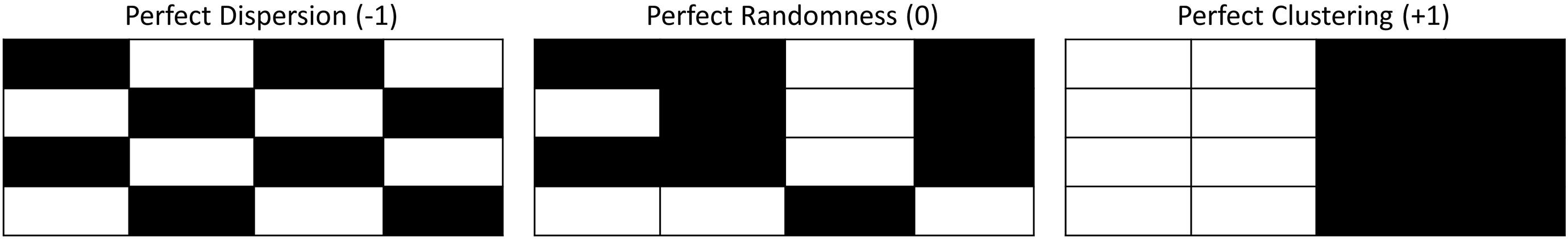
Figure 1. Spatial depiction of ideal Moran’s I values: left- perfect dispersion, Moran’s I value = –1; middle- perfect randomness, Moran’s I value = 0; right- perfect clustering, Moran’s I value = +1.

The Moran’s I statistic is given by the formula (Goodchild, 1986; Odland, 1988):

$$I=\frac{N}{W}\frac{{\sum }_i{\sum }_j{w}_{i,j}(x_i-\overline{x})(x_j-\overline{x})}{{\sum }_i{(x_i-\overline{x})}^2}(1)$$

where $W={\sum }_{i=1}^n{\sum }_{j=1}^n{w}_{i,j}$, w_i,j is the weighting between the ith and jth spatial units, and w represents the weighting matrix with i rows and j columns. x_i refers to the ith feature value, [e.g., the total number of GVP of the ith spatial unit (e.g., hydrophone)], and $\overline{x}$ is the mean of all of a feature’s values (e.g., the mean number of GVP across all hydrophones).

The weighting matrix (w) is a contiguity matrix representing the relationship between each pair of spatial units, e.g., hydrophones (the ith row and jth column). The weighting (w_i,j) determines the contribution that each set of hydrophones (the ith and jth) makes to the final spatial autocorrelation value. For example, a “Queen’s case” (Figure 2) contiguity weighting scheme considers all hydrophones (j) that are directly perpendicular, horizontal, and diagonal to a particular hydrophone (i) to be adjacent neighbors to that hydrophone, while the other hydrophones are not, i.e., $w_{i,j} = \left\{\begin{array}{c}1,ifjadjacenti\\ 0,ifjnotadjacenti\end{array}\right.$. Those hydrophones that are not adjacent neighbors therefore do not contribute (w_i,j= 0) to the Moran’s I statistic. The “Bishop’s case” (Figure 2) only considers hydrophones that are directly diagonal to be adjacent neighbors, while the “Rook’s case” (Figure 2) only considers hydrophones directly perpendicular or horizontal to be adjacent neighbors. In open ocean beaked whale habitat, it was not expected that there would be any restrictions in how a whale would move so the “Queen’s case” was determined to be the most realistic representation of hydrophone adjacency and was employed when testing both the simulated pattern and exemplar data sets. The use of this specific criterion also assumes that the hydrophones are omnidirectional and therefore able to fully capture this expectation. To ensure the Moran’s I values fall within the (–1, +1) scale, the weighting matrix is row-standardized by dividing each row value by the row sum so that the sum of values in each row totals to one.

FIGURE 2

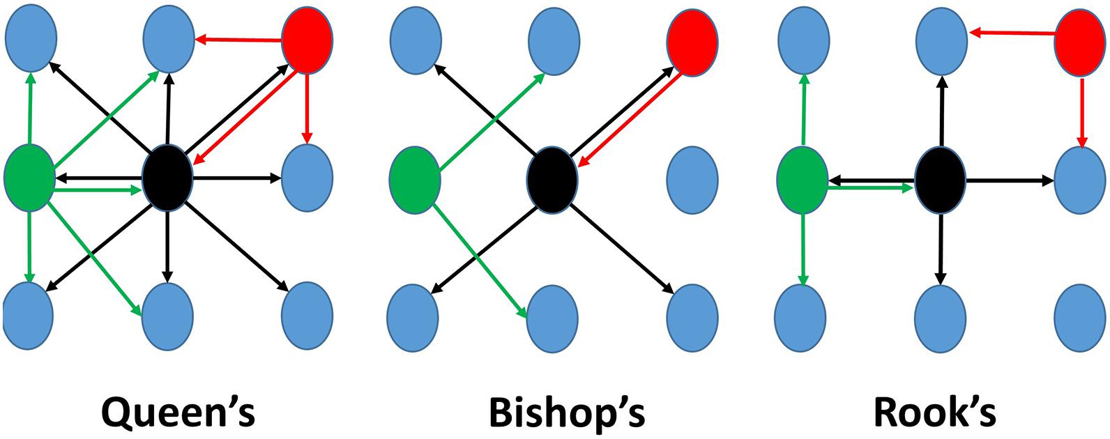
Figure 2. Three examples of contiguity weighting schemes for generating weighting matrices. “Queen’s case” (left) was used in this study, while “Bishop’s case” is in the middle, and “Rook’s case” is on the right. Colored arrows indicate which hydrophones would be considered an adjacent neighbor to the same colored hydrophone. Notice: not all hydrophones will have the same number of neighbors.

To determine if the observed spatial pattern deviates significantly from random (i.e., I = 0) the Moran’s I statistic is converted to a z-statistic (z_I)(Equation 2)with a standard normal distribution upon which significance is determined. The formula for this is given by:

$$z_I=\frac{I-E[I]}{\sqrt{V[I]}}(2)$$

where $E\left[I\right]=\frac{-1}{(n-1)}$ is the expected value for a spatially random distribution and $V\left[I\right]=\frac{A-B}{C}$is the variance of the expected value. Note that the variance of Moran’s I can be calculated based on an assumption of normality, or randomization (Goodchild, 1986; Odland, 1988). The former is appropriate when data follows a normal distribution, but in cases where the distribution is not normal or is unknown, the less restrictive randomization assumption can be used. For skewed data—as is often the case with marine mammal detections and was true in this study—the randomization assumption is more appropriate. This should be reconsidered for the specific application of this statistic. The formula for variance when normality is assumed can be found in Odland (1988). The variance under the randomization assumption is calculated by the following set of equations (Goodchild, 1986; Odland, 1988) (Equations 3–8):

$$A=n[S_1(n^2-3n+3)-n{S}_2+3W^2](3)$$

$$B=D[S_1(n^2-n)-2n{S}_2+6W^2](4)$$

$$C=W^2(n-1)(n-2)(n-3)(5)$$

$$D=\frac{{\sum }_{i=1}^n{(x_i-\overline{x})}^4}{{({\sum }_{i=1}^n{(x_i-\overline{x})}^2)}^2}(6)$$

$$S_1=\frac{1}{2}\sum _{i=1}^n\sum _{j=1}^n{(w_{i,j}+w_{j,i})}^2(7)$$

$$S_2=\sum _{i=1}^n{(\sum _{j=1}^n{w}_{i,j}+\sum _{j=1}^n{w}_{j,i})}^2(8)$$

A p-value is obtained by matching the z-statistic to a standard normal distribution look-up table for the designated level of significance. A 5% significance level (95% confidence level) was used here. The analysis conducted with the Moran’s I statistic is a hypothesis test, where the test hypothesis is that the spatial distribution of the observations is no different from “perfectly” random (I = 0). If the p-value associated with the Moran’s I statistic is less than 0.05, then the distribution is interpreted as statistically different from random: either significantly clustered (I = +1) (Figure 1, right), or significantly dispersed (I = –1) (Figure 1, left).

In the demonstration of the GLC approach, a change in significance of the Moran’s I z-statistic from one analysis period to another is interpreted as a change in mammal behavior globally—e.g., from spatially random to spatially clustered. However, no change would be detected if, for example, all mammals were on the east side of the array as in Figure 1 (right) at time t₁ and moved to the west side at time t₂. Hence, a coupled analysis of behavior at a local scale is necessary.

Local Behavior/Spatial Autocorrelation

The Getis-Ord Gi^∗ statistic (Getis and Ord, 1992) is used to identify pockets of high spatial association, e.g., clustering of similar feature values, or in this demonstration, the number of GVPs. For the remainder of the paper this analysis will be referred to as Gi^∗. The Gi^∗ z-statistic is computed for each spatial unit, or hydrophone, using the following formula (Getis and Ord, 1992):

$$G_i^{*}=\frac{{\sum }_{j=1}^n{w}_{i,j}{x}_j-\overline{X}{\sum }_{j=1}^n{w}_{i,j}}{S\sqrt{\frac{n{\sum }_{j=1}^n{w}_{i,j}^2-{({\sum }_{j=1}^n{w}_{i,j})}^2}{(n-1)}}}(10)$$

where $S=\sqrt{\frac{{\sum }_{j=1}^n{x}_j^2}{n}-{(\overline{X})}^2}$ and $\overline{X}=\frac{{\sum }_{j=1}^n{x}_j}{n}$ and all other variables are as described for the Moran’s I statistic. Note that the use of the Gi^∗ statistic assumes that the data examined are asymptotically normal (i.e., as the number of observations increases the distribution approaches normality) (Getis and Ord, 1992). When using a binary adjacency weighting, such as the queen’s criterion used here, “as long as the distance is not too small and the weights are not too uneven, approximate normality is a reasonable assumption” (Ord and Getis, 1995). Thus in using a contiguity weighting scheme, it is recommended that the number of adjacent sites per feature location be eight or more (Ord and Getis, 1995). This was achieved for interior hydrophones in the array.

Using a two-tailed test, a p-value is determined and used to identify and interpret areas of either high and/or low feature values, e.g., number of GVPs. In particular, a significant hot spot—a non-random cluster of high feature values–will be identified if any hydrophone has a very high z-statistic (> +1.96, or 2 standard deviations) and associated p-value ≤ 0.025, while a significant cold spot –a non-random cluster of low values–will be identified if any hydrophone has a very low z-statistic (< –1.96, or 2 standard deviations) and associated p-value ≥ 0.975. Clusters of high and low feature values are used to track how spatial behavior changes on the array through subsequent analysis periods.

Examining locational changes of areas of clustering from one analysis period to the next, provides insight into spatial behavior not captured by the global Moran’s I result. In the exemplars, if all mammals move from the east to the west from one period to the next, as described earlier, a clear change in the location of hot and cold spots would be observed which would not have been detected by using only the global Moran’s I statistic.

Comparison Analysis

Each spatial statistic takes into account the distribution and variance of only a single set of observations from one unit of time, or analysis period. Since the distribution and variance of a feature (e.g., number of GVPs) can change across analysis periods, it is not appropriate to compare the spatial statistic (i.e., Moran’s I or Gi^∗) values across analysis periods (i.e., a comparison of a Moran’s I value of 0.2 for one period to a Moran’s I value of 1.2 in another period is meaningless if the distribution and variance of each period is different). In addition, the Gi^∗ z-statistic is scale-invariant (Ord and Getis, 1995), meaning the same results may occur for a similar pattern despite a different range of feature values for two or more analysis periods. For example with beaked whale foraging behavior, neither Moran’s I nor Gi^∗ will detect that there has been a substantial change if there are two analysis periods where the hot spot cluster remains in the western corner of the array. But if one cluster has 30 GVPs, while in the next analysis period the cluster only has one GVP, a substantial change has occurred. This would be detected by comparing the order-of-magnitude across analysis periods. A comparison test is necessary for determining if the number of observations across analysis periods has changed (i.e., do the two samples come from a similar population or not). It is recommended that statistical test-specific assumptions be evaluated to decide the most appropriate statistical hypothesis comparison test to use for a specific data set.

Here, the non-parametric Kruskal-Wallis test (Kruskal and Wallis, 1952) was used to compare the data sets of spatial observations (i.e., the number of GVPs per hydrophone) in the different analysis periods. The test hypothesis in the Kruskal-Wallis test is that the samples come from similarly shaped distributions (Kruskal and Wallis, 1952). However, the test does not assume that the data are normally distributed, which is the primary driver for its use here. The distribution of the number of GVPs per hydrophone was skewed, with many hydrophones having zero observations. One other assumption of the Kruskal-Wallis test is that the samples compared are independent (i.e., both in and across analysis periods). The exemplar data sets were assumed to be independent as both temporal and spatial autocorrelation were tested and found to be low or non-existent in the original studies (McCarthy et al., 2011; Manzano-Roth et al., 2016).

The Kruskal-Wallis test works by ranking the observations in each analysis period and comparing the mean ranks of each (Kruskal and Wallis, 1952). A significance level is used to statistically identify the compatibility between the observed data and what is expected under the test model and its assumptions (Greenland et al., 2016). For ease in interpretation, a 5% significance level (α = 0.05) was used here. A p-value smaller than 0.05 suggests that the data are rare under the model, in other words, that the samples come from different distributions, while a p-value larger than 0.05 suggests the data are not unusual under the model, or that the samples come from similar distributions. If differences in the number of spatial observations (i.e., number of GVPs) across analysis periods are detected, a post-hoc multiple comparison test is used to determine which analysis periods are different from one another. Here, Tukey’s honest significant difference criterion was used due to its effectiveness with data of equal sample sizes (i.e., there were 89 observations, one for each hydrophone, per analysis period) (The MathWorks Inc, 2020). A significance level of 5% was used again to interpret which analysis periods differed from one another.

Finally, difference plots are generated to show the relative change (e.g., increase, decrease, or no change) in the number of observations on a per hydrophone basis between consecutive analysis periods. It is worth noting that the difference plots are based on binary rather than continuous values; a hydrophone that has a change of positive 1 between two periods will be represented the same as a hydrophone that has a change of positive 0.1 from one period to the next. Thus, these plots, as well as visualizing the original data, are only used to aid in the interpretation of the spatial statistics.

Note that the choice of statistical hypothesis test and post-hoc test may vary depending on the nature of the data. For example, if the data follow a normal distribution and satisfy the other assumptions of a parametric test, a test such as the analysis of variance (ANOVA) can be more powerful, although Andrews (1954) found the Kruskal-Wallis test to have a power efficiency of 0.955 relative to the parametric ANOVA’s F-test.

Data

Simulated Data Sets

Several patterned GVP data sets were created and tested to reveal how this approach would perform on known types of spatial distributions. The types of spatial distributions tested were chosen because they represent simple but realistic patterns of what might be expected of marine mammal foraging. This was conducted on a mock 50 “hydrophone” (10 row by 5 column) equi-spaced array. The simulated GVP data sets included seven patterned data sets (Alternate, Diagonal, Striped, Steep Grade, Graded, Cluster, and Graded Cluster) and three randomly generated data sets (Random 1–3). The ten simulated data sets tested are shown in Figures 3, 4, column 1. These figures will be introduced in full in the Results section. The Alternate, Diagonal, Striped, and Cluster pattern data were all generated using hydrophone values of zero (to represent a low value) or ten (to represent a high value) only to ensure the pattern was clear and not confounded by varying degrees of low and high values. For the Alternate pattern, every other hydrophone was either a zero or a ten so that no two hydrophones next to one another in the horizontal or vertical direction would have the same number, though they would diagonally. The Diagonal pattern consisted of three diagonal rows of zeros while the values of the remaining hydrophones were ten. The Striped pattern consisted of five alternating columns of ten hydrophones with a value of either zero or ten. The Steep Grade pattern consisted of five columns with values of ten, seven, four, zero, five, moving from left to right, while the Graded pattern consisted of five columns with values of ten, nine, eight, seven, eight, from left to right. The Cluster pattern consisted of a set of three by three hydrophones each with a value of ten in the center of the array and zeros for the remaining hydrophones. The Graded Cluster pattern included the same cluster pattern in the center of the array with a surrounding ring of hydrophones around this cluster with value of five and the remaining hydrophones with value zero. The three random data sets were randomly generated integer values between zero and ten for each of the 50 hydrophones.

FIGURE 3

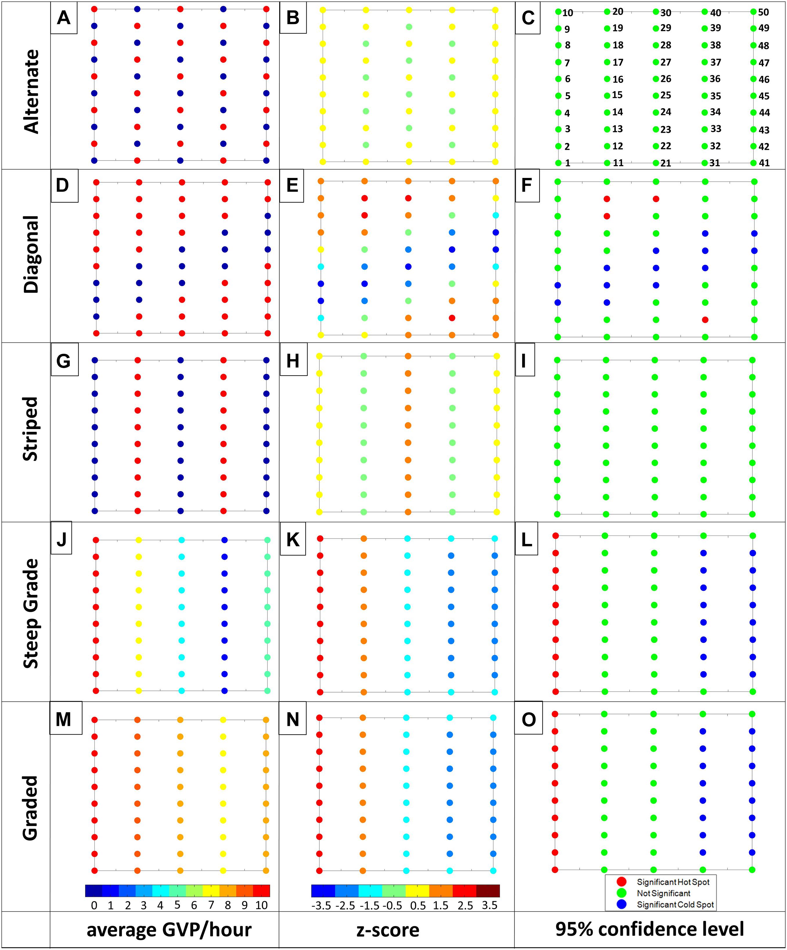
Figure 3. Visualization of the Gi* results for the Alternate, Diagonal, Striped, Steep Grade, and Graded Patterns (top to bottom). From left to right: first column: average GVP per hour with color bar ranging from 0 (dark blue) to 10 (red); second column: Gi* z-statistic with color bar ranging from –3.5 (dark blue) to 3.5 (dark red); third column: 95% confidence level, where red indicates a significant hot spot and blue indicates a significant cold spot, while green is not significant. For ease in displaying, individual hydrophone values were rounded to the closest number on the color bar for columns one and two. The numbers provided on Figure 3C correspond to hydrophones discussed in the Results. Letters associated with each plot are used for ease in referencing individual plots in the text.

FIGURE 4

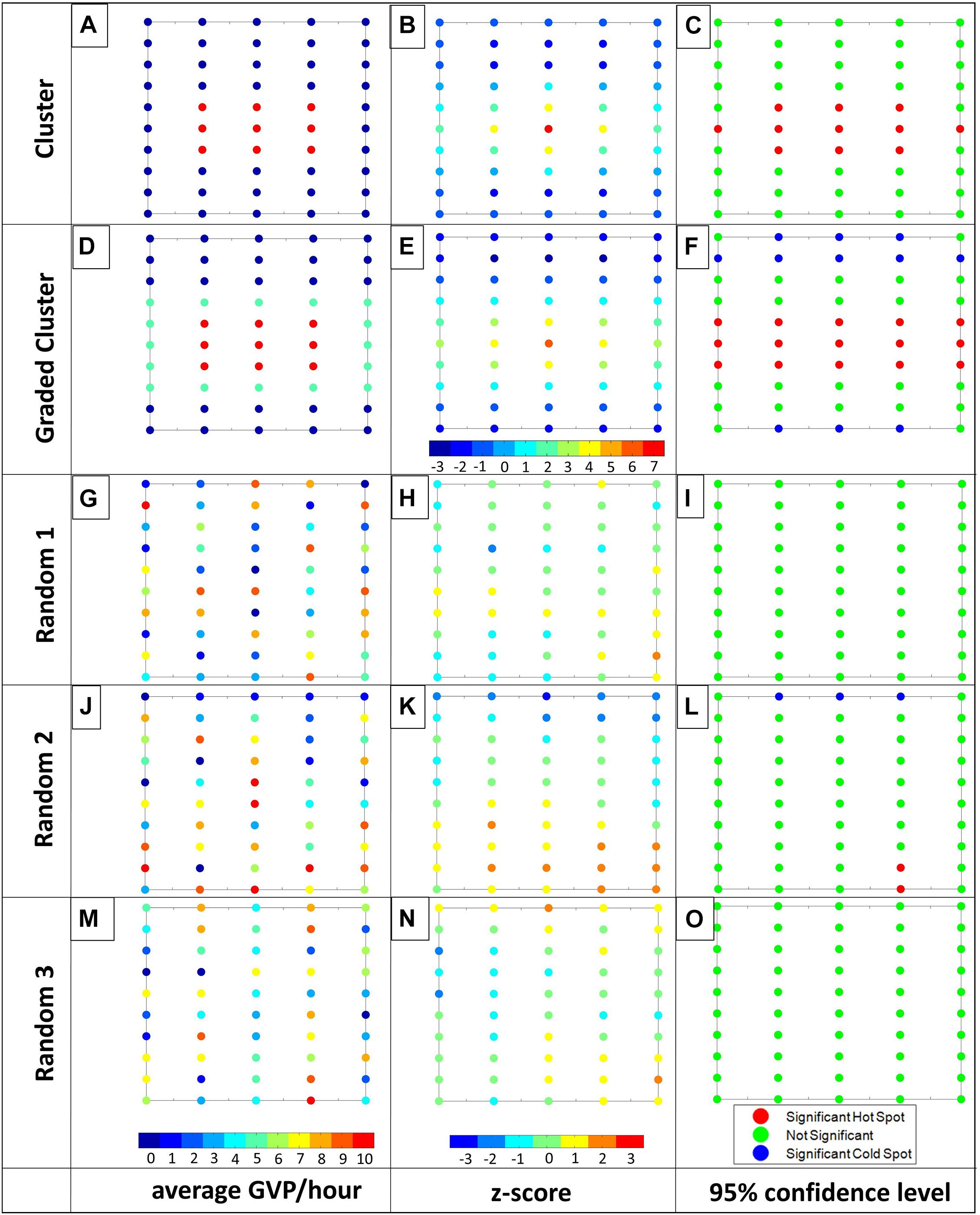
Figure 4. Visualization of the Gi* results for the Cluster, Graded Cluster, Random 1, Random 2, and Random 3 patterns (top to bottom). From left to right: first column: average GVPs per hour with color bar ranging from 0 (dark blue) to 10 (red); second column: Gi* z-statistic with color bar ranging from –3 (dark blue) to 7 (red) for the Cluster and Graded Cluster patterns and from –3 (dark blue) to 3 (red) for the random arrangements; third column: 95% confidence level, where red indicates a significant hot spot and blue indicates a significant cold spot, while green is not significant. For ease in displaying, individual hydrophone values were rounded to the closest number on the color bar for columns one and two. Letters associated with each plot are used for ease in referencing individual plots in the text.

Specific to the Moran’s I statistic, the Alternate design was hypothesized to represent a scenario of dispersed foraging (i.e., I < 0), while the remaining simulated patterns were hypothesized to represent different configurations of clustered foraging (i.e., I > 0). The random data sets were hypothesized to show spatial patterning no different from random (i.e., I = 0). The Gi^∗ results were hypothesized to statistically identify the areas of high and low GVP activity (hot and cold spots, respectively) intentionally designed into each of the simulated spatial patterns. For example, it was expected that the Diagonal pattern, consisting of low values in a diagonal pattern across the array would lead to a diagonal pattern of cold spot hydrophones in the same location as the low GVP values. It was expected that the cluster of high values in the center of the Cluster and Graded Cluster patterns would be identified as a cluster of hot spots in the Gi^∗ analysis. It was also hypothesized that there would be a noticeable difference in the resulting Gi^∗ values and significance, for the Steep Grade vs. the Graded patterns, as well as the Cluster vs. Graded Cluster patterns due to differences in grading, despite the similar overall pattern within these two sets of patterns. The random patterns were expected to show no significant hot or cold spots.

Exemplar Studies

The data from two previously published marine mammal behavior studies were extracted and tested to demonstrate how the GLC approach performed on empirical spatial behavior data. One study assessed Blainville’s beaked whale foraging behavior during mid-frequency active sonar (MFAS) Naval exercises in 2007 on the Atlantic Undersea Test and Evaluation Center (AUTEC) in the Bahamas (McCarthy et al., 2011). The AUTEC study compared foraging intensity Before, During, and After MFAS activity on an 82 hydrophone array. The second study involved the same species and MFAS exposure between 2011 and 2013 on the Pacific Missile Range Facility (PMRF) off of Hawaii (Manzano-Roth et al., 2016). The PMRF study compared foraging intensity Before, During Phase A, During Phase B, and After Navy sonar activity on a 62 hydrophone array. The difference between the two During phases of the PMRF study was that Phase A only included submarine-on-submarine activity without MFAS, while Phase B used surface ship MFAS, sonobuoys, and dipping sonars (Manzano-Roth et al., 2016). The length of and timing between analysis periods of the two studies was on the order of hours to days. For more specific details on the activities and characteristics of the analysis periods in these studies, see the respective publications (McCarthy et al., 2011; Manzano-Roth et al., 2016). In both studies, the authors performed a visually quantitative spatial assessment generating the heat maps of GVP activity reproduced in Figure 5. The intention in using the McCarthy et al. (2011) and Manzano-Roth et al. (2016) data was not to serve as a reanalysis of those efforts, but rather specifically to demonstrate the GLC approach on an empirical data set. If one is explicitly interested in the effect of MFAS on beaked whale behavior, the McCarthy et al. (2011) and Manzano-Roth et al. (2016) papers should be reviewed.

FIGURE 5

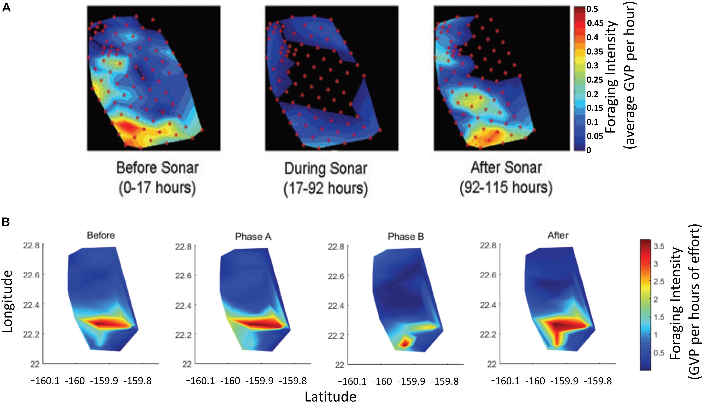
Figure 5. (A) Reproduced from Figure 6 in McCarthy et al., 2011, which shows the foraging intensity, as the average GVP per hour, of Blainville’s beaked whales on the AUTEC hydrophone array Before, During, and After MFAS activity. Red circles indicate positions of the hydrophones in the McCarthy et al., 2011 study. Colorbar values and label have been rewritten for legibility from original figure. (B) Reproduced from Figure 3 in Manzano-Roth et al., 2016, which shows the foraging intensity in GVP per hours of effort of Blainville’s beaked whales on the PMRF array Before, during Phase A, during Phase B, and After Naval sonar activity. Color bar label has been added and was not present in original figure.

Since the original data from the McCarthy et al. (2011) and Manzano-Roth et al. (2016) studies were not available for use in this study due to military data access, foraging intensity values were visually extracted from the heat maps (Figure 5). Note that both studies display the foraging intensity, but the AUTEC metric units (McCarthy et al., 2011) were GVPs per hour, whereas the PMRF metric units were GVPs normalized by the total hours of effort (Manzano-Roth et al., 2016). Thus, there was an order of magnitude difference between the data values of the two studies. In this study, white grid lines were overlaid on the AUTEC and PMRF data images (Figure 6), and the value at each grid intersection was visually extracted. Values at the white grid locations indicated by a yellow “x” were ignored to achieve a similar number of hydrophone observations as the original studies (Figure 6). These grid patterns were designed to provide a representative sampling of the original study area. However, the heat maps in the original studies were generated using interpolation between hydrophones, so the extracted values do not necessarily align with the hydrophone data values of the original studies. The extracted values were then associated with a mock hydrophone array with 84 hydrophones for the AUTEC exemplar (Figure 6, top) and 62 for the PMRF exemplar (Figure 6, bottom). The mock arrays were designed to mimic the original array designs, with staggered rows and a similar number of rows and columns to the original hydrophone arrays. The actual layouts of the AUTEC and PMRF hydrophone arrays deviate from this simplified design. Rather than matching the precise layouts of the AUTEC and PMRF arrays, the simplified designs were chosen because the purpose of this study was a proof-of-concept and demonstration of the GLC approach rather than definitively quantifying the spatial behavior of beaked whales on AUTEC and PMRF during those studies. The extracted data and neighbor-weighting matrices generated for both the AUTEC and PMRF exemplars can be found in the Supplementary Material. It was hypothesized that for the AUTEC exemplar, the Moran’s I analysis would show spatial clustering for all three periods (Before, During, After), but that the Gi^∗ analysis would reveal a cluster of hot spot hydrophones in the southwest corner of the array Before, a cluster of cold spot hydrophones in the middle of the array During, and a hot spot cluster again in the southwest corner of the array After Navy MFAS activity. For the PMRF exemplar, it was hypothesized that the Moran’s I analysis would show spatial clustering for all four analysis periods (Before, Phase A, Phase B, After), but that the Gi^∗ analysis would reveal a change in where the clustering took place on the array. In particular, During Phase B and After the hot spot of activity would shift southward on the array, and a cold spot of activity would be located in the center of the array During Phase B.

FIGURE 6

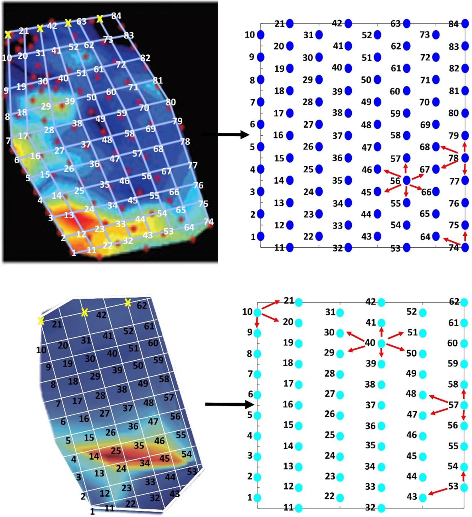
Figure 6. Schematic of how the data were extracted from the heat maps in the original studies (left figures) –AUTEC (top) and PMRF (bottom)—and mapped onto the mock hydrophone arrays (right figures). For this study the white grid lines were added to each of the analysis period data images in Figure 5. The values at the grid intersections were extracted to create the exemplar data sets. Gridlines marked by a yellow “x” indicate values that were not extracted. Each circle on the right represents the location of a hydrophone on the mock arrays. The numbers in the left figures correspond to the same number in the right figures and show where the value on the heat map was extracted from and to. In addition, the right figures provide examples of adjacent neighbor assignments for each of the hydrophone array layouts. Red arrows point to hydrophones that would be considered an adjacent neighbor to the respective hydrophone centered within the arrows.

Results

Simulated Data Sets

The Moran’s I analysis results including the Moran’s I value, z-statistic, and p-value are shown for the seven patterns and three randomly generated data sets in Table 1. The Diagonal, Steep Grade, Graded, Cluster, Graded Cluster, all exhibited significant spatial clustering as expected. In addition Random 2 was also significantly clustered, contrary to expectation, while Random 1 and Random 3, as expected, could not be statistically differentiated from a random spatial distribution. The Alternate and Striped patterns were statistically no different from random, which was also not expected.

TABLE 1

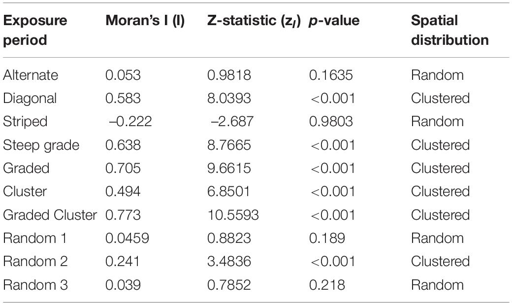
Table 1. Moran’s I analysis results by exposure period for the patterns and random data sets, including Moran’s I value (I), the z-statistic (z_I), and the associated p-value.

Despite some of the unexpected Moran’s I results, with all ten simulated data sets the Gi^∗ analysis corroborated the findings of the Moran’s I analysis (Table 1) and provided further insight into the results. The spatial pattern of the Gi^∗ z-statistics and significance results (Figures 3, 4, columns 2 and 3) matched intuitively to the values in the original pattern. For every clustered pattern, clusters (i.e., several hydrophones next to one another) of hot spots and/or cold spots were identified, while for every random pattern only a few or no hot/cold spot hydrophones were detected. As an example, in the graded patterns (i.e., Steep Grade and Graded) the highest number of GVPs were on the western hydrophones and lowest were on the eastern hydrophones of the array. The Gi^∗ analysis identified a column of hot spots in the western-most column and cold spot hydrophones in the eastern-most two columns.

The results of the Gi^∗ analysis of the Alternate and Striped patterns provided further insight into the unexpected result of the Moran’s I analysis that showed these patterns had a random distribution. These patterns had low z-statistic variability with values that deviated little from the mean (Figures 3B,H, respectively). Because of the narrow range of z-statistic values, both patterns were non-significant and no hot or cold spots were identified (Figures 3C,I). The lack of z-statistic variability can be explained by the fact that each hydrophone was surrounded by roughly the same number of high and low value neighbors and there was no variability in what those high and low values were (either ten or zero). The exception to this was the middle column in the Striped pattern that was surrounded by high values on either side thereby producing a larger z-statistic for the middle hydrophones of the pattern. A random result for Moran’s I and non-significant result for the Gi^∗ analysis suggest that the observable patterns in these examples were not sufficiently pronounced to be detected statistically with this analysis.

The spatial distribution of the hot/cold spot hydrophones in the simulated patterns that were identified by the spatial analysis as clustered (i.e., Diagonal, Cluster, Graded Cluster, Steep Grade, and Graded) generally overlapped the designed observable pattern (e.g., a diagonal pattern of cold spot hydrophones was indeed present on the hydrophone array in the Diagonal example). However, with each pattern there were a few exceptions. For example in the Diagonal pattern, there was a cold spot cluster of hydrophones almost entirely overlapping the area of the zero-valued diagonal pattern (Figure 3F), with the exception of two perimeter hydrophones (hydrophones 3 and 48) which were not identified as cold spots, despite being a part of the original diagonal pattern. As another example, the entire cluster plus the two middle hydrophones on the lateral edges of the cluster (hydrophones 5 and 45) were identified as significant hot spots in the Cluster pattern (Figure 4C). There were similar cases of this in the other clustered patterns where some hydrophones were or were not identified as being significant hot/cold spots, despite what one may expect based on visual expectation. This was an effect of the neighbor-weighting aspect of the Gi^∗ z-statistic calculation. Edge hydrophones generally have fewer neighbors, meaning the value of those neighbors has a greater weight in comparison to the neighbors of hydrophones in the center of the range and therefore a different contribution to the z-statistic calculation.

The matching Gi^∗ spatial distribution of hot and cold spots for the Steep Grade and Graded patterns (Figures 3L,O) exemplified the scale-invariant nature of the Gi^∗ analysis. There were no obvious differences between the two patterns upon which the magnitude difference between the two patterns could be differentiated, supporting the need for the comparison analysis when comparing two data sets or analysis periods.

For the three random patterns the spatial distribution of the Gi^∗ z-statistic values appeared random, except for Random 2 which had a more graded pattern with high Gi^∗ z-statistic values toward the south and southeast corner and a row of low values along the northern perimeter of the hydrophone array (Figure 4K). As a result, two hot spot hydrophones were identified in Random 2 near the southeast corner of the array and three cold spot hydrophones were identified along the northern perimeter of the array (Figure 4L). There were no hot or cold spot hydrophones identified in Random 1 or 3 (Figures 4I,O, respectively), matching the Moran’s I result that these patterns were random.

To further explore the likelihood of the Random 2 results, an ad hoc simulation test was run to compute the Moran’s I analysis on 1,000 randomly generated data sets. On average, the Moran’s I value was 0.1283, the z-statistic was 2.0583 (SD = ± 0.88), and the p-value was 0.0587 (SD = ± 0.09). Based on a 5% significance level, a random data set would, on average, not result in statistical significance and therefore would be interpreted as no different from random. However, implicit in the use of a significance level to detect statistical significance, is the acceptance that there may be times when the data do not match the underlying model. Thus on an array of 50 hydrophones and a 5% significance level, it is acceptable that 5%, or 2.5 hydrophones, may be identified as hot or cold spots despite an underlying random distribution, which the Random 2 pattern demonstrates.

Exemplar Studies

Atlantic Undersea Test and Evaluation Center Exemplar

Visual interpretation of the GVP data (Figure 7, column 1) indicated that Before MFAS activity the most GVPs occurred on hydrophones in the southwest corner of the array. During MFAS activity there were very few GVPs on the array compared to the Before period and the few GVPs that were present appeared highest along the edges of the array. After MFAS activity the level of activity appeared to match the Before period, with a shift toward the south-center of the array.

FIGURE 7

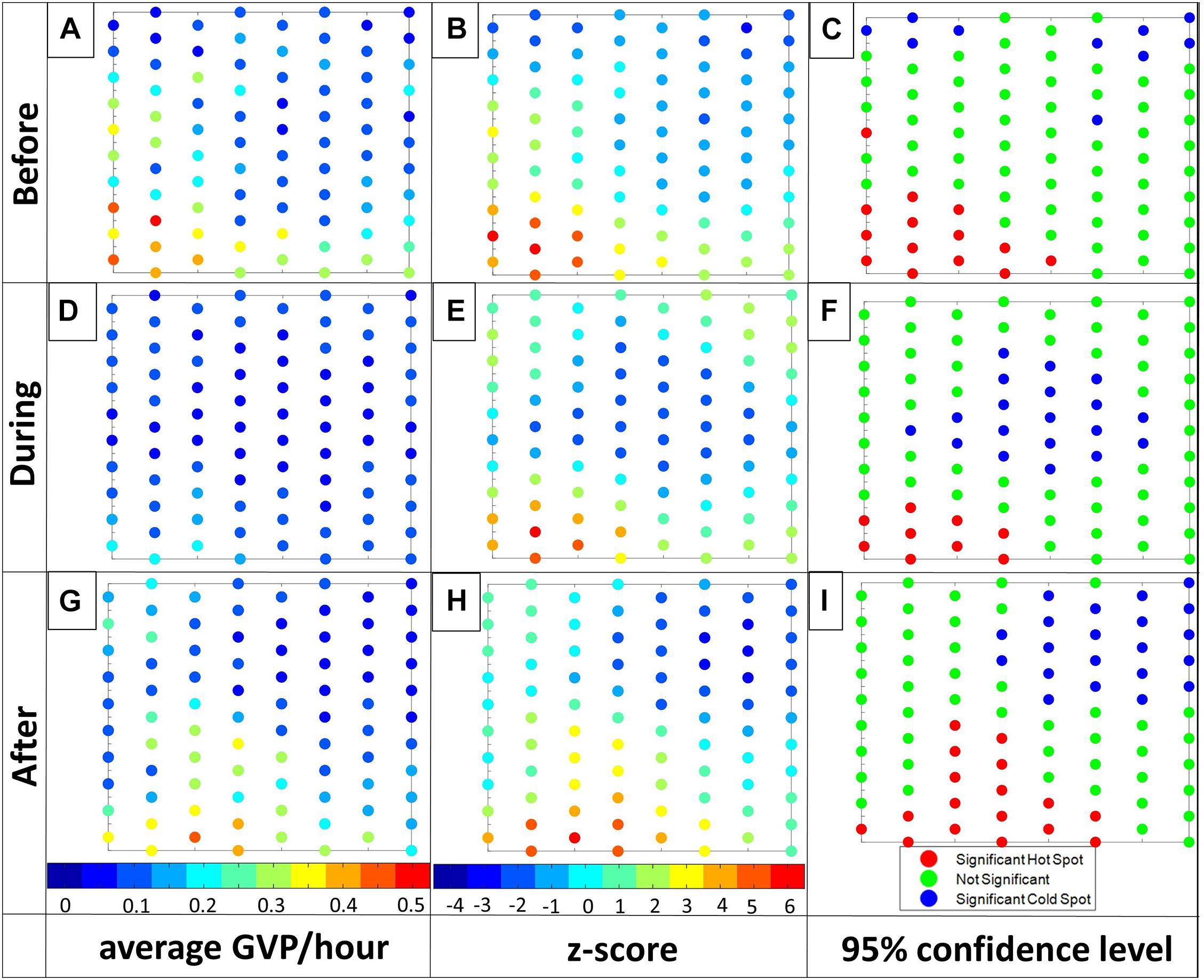
Figure 7. Visualization of the Gi* results for the AUTEC exemplar: Before, During, and After, from top row to bottom row, respectively. From left column to right: 1) the average GVP/hour with colorbar ranging from 0 (dark blue) to 0.5 (red) GVP/hour, 2) the Gi* z-value with colorbar ranging from –4 (dark blue) to 6 (red), and 3) hot (red) and cold spots (blue) at a 95% confidence level. Note: For ease in displaying, individual hydrophone values were rounded to the closest number on the color bar for columns one and two. Letters associated with each plot are used for ease in referencing individual plots in the text.

The Moran’s I, z-statistic, and p-value component of the GLC approach for Before, During, and After in the AUTEC study are listed in Table 2 below. The Moran’s I values all suggest clustering of GVP activity on the array in each analysis period. From an array-wide perspective, there was no clear change in global foraging behavior.

TABLE 2

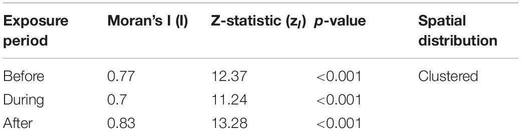
Table 2. Moran’s I analysis results by analysis period for the AUTEC exemplar, including Moran’s I value (I), the z-statistic (z_I), and the associated p-value.

The Gi^∗ portion of the GLC analysis corroborated the results of the Moran’s I test since both hot and cold spot hydrophone clusters were found in all analysis periods. In particular, a cluster of hot spot hydrophones were identified by the Gi^∗ analysis in the southwest of the array for each analysis period (Figures 7C,F,I). The exact location and number of hot spot hydrophones did vary from period to period, but drawing upon the results of the simulated patterns, some variation is expected due to the neighbor-weighting component of the analysis. The GLC approach consistently identified a cluster of hot spot hydrophones in the southwest of the array that accords with a visual assessment, suggesting that the animals continued to forage predominantly in the same area throughout all analysis periods. The significance test of the Gi^∗ analysis also revealed a cluster of cold spots in each of the analysis periods, which clearly changed location on the array from one analysis period to the next. Before, there were only a few cold spot hydrophones along the northern perimeter of the array; During, there was a large cluster of cold spot hydrophones in the center of the array; After there was a large cold spot cluster in the northeastern corner of the array (Figures 7C,F,I). In both the During and After periods there were roughly double the number of cold spot hydrophones compared to the Before period. These cold spots were also all clustered together, unlike in the Before period where they were more spaced out along the northern perimeter (Figure 7C). The results of the Gi^∗ portion of the GLC approach suggest there was a change in where GVP activity was absent on the array During MFAS activity. It also shows that there was an increase in the number of hydrophones upon which no GVP activity took place.

As discussed, the Moran’s I and Gi^∗ statistics alone do not confirm the change in overall activity. Hence the ability to detect changes in the global level of activity through the comparison test is an integral part of the GLC. The Kruskal-Wallis test showed that there was a difference across the mean ranks of the analysis periods [H(2) = 48.48, p = 2.97 × 10^–11]. The post-hoc test showed that there were fewer (p < 0.001) GVPs on the array During MFAS activity than Before or After. So although the location on the array with the highest foraging activity (i.e., hot spot cluster) relative to a particular analysis period did not change, the absolute number of foraging events within a period did change. The difference plots supported this finding; there was a decrease in the number of GVPs on most of the hydrophones from Before to During and an increase or no change in the number of GVP from during to After (Figure 8). Due to the scale-invariant nature of the Gi^∗ statistic and the global nature of the Moran’s I analysis, this overall understanding about the spatial behavior and magnitude of change was not completely realizable through the spatial statistics alone. This emphasizes the importance of considering each of the three parts to the GLC approach in interpreting and understanding spatial behavior change.

FIGURE 8

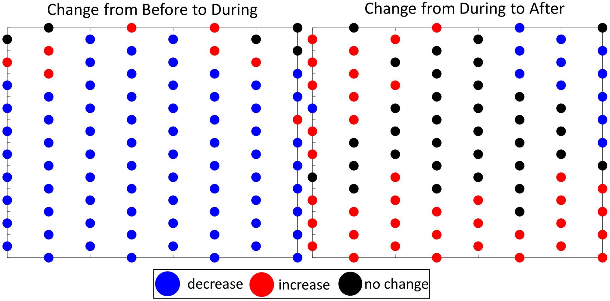
Figure 8. Spatial layout of mock AUTEC hydrophone array, where the circles represent the hydrophones of the array, and the color represents the change in the number of GVP on each hydrophone from one analysis period to the next: blue = decrease, red = increase, black = no change. Left- the change from Before to During MFAS activity, and Right- the change from During to After MFAS activity.

Pacific Missile Range Facility Exemplar

A visual analysis of the PMRF exemplar revealed that the most GVP activity appeared in the top part of the southern half of the array. During Phase B and After, there was a shift southward in where the most activity occurred in comparison to the earlier periods (i.e., there was also high GVP activity along the bottom southwest edge of the array). The least amount of GVP activity appeared to be along the southern edge of the array Before, but then shifted to the northern edge of the array during Phase A, and then to the center of the array during Phase B and After (Figure 9, column 1).

FIGURE 9

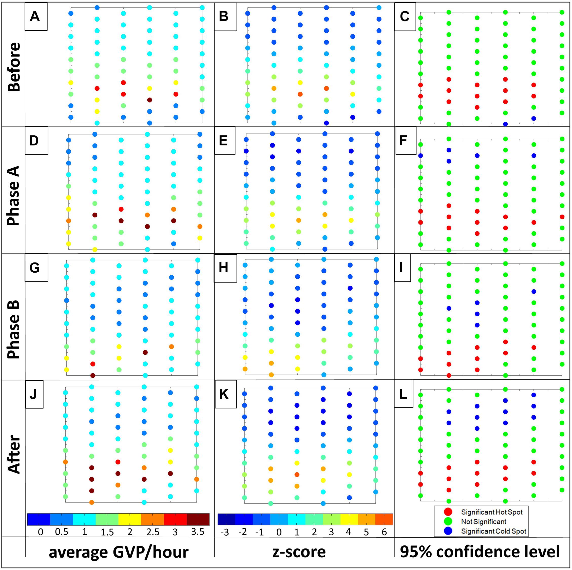
Figure 9. Visualization of the Gi* results for the PMRF exemplar: Before, Phase A, Phase B, and After, from top row to bottom row, respectively. From left column to right: (1) the average GVP/hour standardized to total time where the colorbar ranges from 0 (dark blue) to 3.5 (red) GVP/hour the Gi* z-value with colorbar ranging from –3 (dark blue) to 6 (red), and 3) hot (red) and cold spots (blue) at a 95% confidence level. For ease in displaying, individual hydrophone values were rounded to the closest number on the color bar for columns one and two. Letters associated with each plot are used for ease in referencing individual plots in the text.

The Moran’s I values, associated z-statistics, and p-values for Before, Phase A, Phase B, and After are listed in Table 3. For all analysis periods of the PMRF study, the Moran’s I results suggested significant spatial clustering of GVP activity, or lack of activity, on the array. From the Moran’s I analysis alone there was no indication that the beaked whales changed their global foraging behavior on the array.

TABLE 3

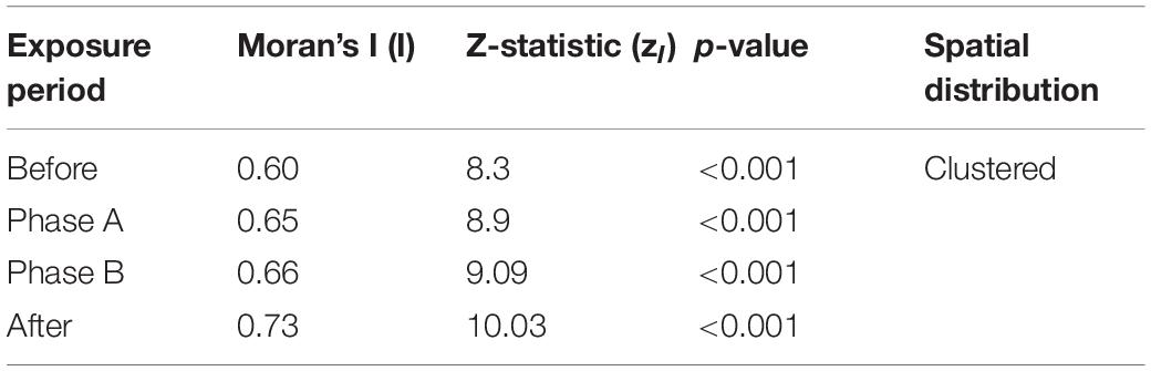
Table 3. Moran’s I analysis results by analysis period for the PMRF exemplar, including Moran’s I value (I), the z-statistic (z_I), and the associated p-value.

The Gi^∗ analysis provided further insight about the clustering result of the Moran’s I portion of the GLC approach analysis. There were clusters of hot and cold spot hydrophones identified in each of the analysis periods. In all four periods there was a large cluster of hot spot hydrophones that spanned across nearly all columns in the southern half of the array (Figure 9, column 3). However, the Phase B period was the only period in which hot spots were identified on some of the southern perimeter hydrophones. Though there were differences in the exact hydrophones that were identified through the GLC analysis as hot spots, based on this information alone, there was no compelling reason to suggest these differences were outside of the variation expected due to natural variation in behavior, or due to the sensitivity in the GLC analysis, discussed previously.

Overall the Gi^∗ z-statistic plot for each period had a similar appearance: lower values dominated the northern half of the array (Figure 9, column 2), suggesting this area was consistently not used for foraging. There were subtle differences in how far this low-value space extended. In particular, it was confined mostly to the northern half of the array Before (Figure 9B), but extended further south in Phase B (Figure 9H). In terms of significance, the GLC approach identified five or fewer hydrophones as cold spots in the first three analysis periods, while in the After period a more substantial cluster of 11 cold spot hydrophones was identified. In addition, the cold spots moved from the southern perimeter of the array Before to a more northern location during Phase A, and a more central location of the array during Phase B and After. These results closely matched the visual assessment and suggest that the animals may not have used the middle of the array as widely during these periods as they did Before.

Using the spatial statistics of the GLC approach alone, it was difficult to tell whether the small changes in location of hot spots were an actual change in spatial behavior over the array or within the natural variation to be expected in marine mammal behavior. It is also possible that the resolution of the hydrophone spacing was not fine enough to fully capture the potential spatial behavior change—a danger present in all spatial studies. However, the comparison analysis provided further insight. The Kruskal-Wallis test revealed that there was a difference in the mean ranks of the four analysis periods [H(3) = 9.53, p = 0.0231]. The post-hoc test showed that there were fewer GVPs on the array overall during Phase B compared to Phase A (p = 0.043) and After (p = 0.035). This finding was also corroborated visually in the difference plots which showed the center of the array had an overall decrease in GVP activity from Phase A to Phase B, but had an increase again from Phase B to After (Figure 10). The results of the comparison portion of the GLC approach provided support that a change in spatial behavior did occur. There were fewer animals foraging and the location of foraging shifted southward during Phase B. This exemplar of the GLC approach further highlights the value of using all three analyses of the GLC approach together to fully understand group level spatial behavior change. It also draws attention to the importance of having the correct spatial resolution to be able to identify spatial behavior patterns.

FIGURE 10

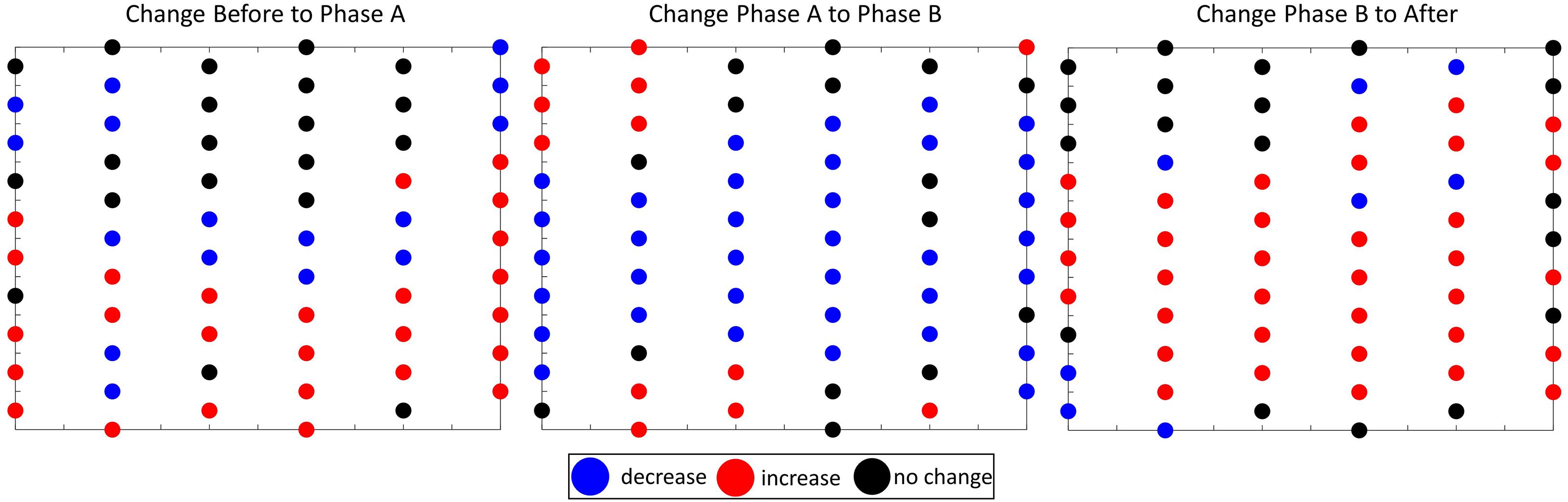
Figure 10. Spatial layout of PMRF hydrophone array, where the circles represent the hydrophones of the array, and the color represents the change in the number of GVP on each hydrophone from one analysis period to the next: blue = decrease, red = increase, black = no change. Left- the change from Before to Phase A, Middle-the change from Phase A to Phase B, and Right- the change from Phase B to After.

Discussion

The results of the spatial analysis for the simulated data sets offered unique insight into how the GLC approach performed and provided guidance on how to interpret the more complex results of the empirical exemplars of group level marine mammal spatial detections representing foraging behavior. The results of the exemplar data sets conveyed the importance and necessity of using all components of the GLC approach together to achieve a comprehensive understanding of spatial behavior patterns. Moreover, the weakness of examining individual statistics in isolation of the others was demonstrated. When the underlying mechanism of the spatial pattern is not known, the insight gained in this three-pronged approach, along with knowledge of the context, can help support or refute potential hypotheses explaining the observations.

Several instances arose within the simulated data sets where edge hydrophones were either non-intuitively identified or not identified as being significant by the Gi^∗ analysis of the GLC approach in comparison to the visual assessment of the original data. For example, the Gi^∗ analysis of the Diagonal pattern did not identify some perimeter hydrophones that made up the diagonal pattern as significant, while in the Cluster pattern some hydrophones outside of the cluster pattern were significant. This is because edge hydrophones have fewer neighbors than center hydrophones, so the contribution of each neighbor in the edge hydrophone case, has a larger weight in the Gi^∗ statistic calculation than in the case of a center hydrophone (Ord and Getis, 1995). This has important implications in analyzing hydrophone arrays that are long and narrow rather than square or circular. This is also an important aspect to keep in mind when choosing the number of hydrophones in the array. For example, in a square array of only four hydrophones the weighting contribution of all neighbor hydrophones would be the same, but in a square of 16 hydrophones, all but the center four would be considered “edge” hydrophones. The edge hydrophone effect will occur with any of the contiguity weighting schemes shown in Figure 2. However, if the weighting scheme is more constrained (i.e., choosing “Rook’s” over “Queen’s”), the edge hydrophone calculation will be different (i.e., a more constrained neighbor scheme means less neighbors and less neighbors equates to a higher weight for each neighbor in the overall calculation) in comparison to a center hydrophone, than if the weighting is less constrained (i.e., “Queen’s” over “Rook’s”) (Ord and Getis, 1995). This is an important aspect of the calculation to consider when interpreting the outcome of the GLC Gi^∗ significance test using an adjacent neighbor weighting scheme. When using a similar weighting scheme it is recommended that the general area of hot/cold spot hydrophone clusters be compared rather than scrutinizing differences between individual hydrophones. Alternatively, a distance weighting scheme can be used, where every pair of hydrophones within some distance of the hydrophone of interest is represented in the Gi^∗ calculation for that hydrophone. As the distance from the hydrophone of interest increases, the contribution of other hydrophones (i.e., the weighting coefficient) toward the Gi^∗ value decreases. It is therefore possible to minimize the edge effect (i.e., ensure all hydrophones have the same number of neighbors) using this scheme, since the number of weights is no longer a function of edge vs. non-edge hydrophone, but rather a function of distance. Whether this is realized would depend on the exact parameter (i.e., distance threshold) and array layout used. A distance weighting scheme is especially appropriate for observations that change on a gradient. This was not assumed to be the case for beaked whale foraging behavior, which is strongly linked to–often patchy and heterogeneous–prey distributions (Benoit-Bird et al., 2013; Southall et al., 2018).

The type of neighbor-weighting rule can also have significant implications on the overall outcome of the Moran’s I statistic. The Moran’s I analysis of the simulated pattern data sets revealed that it was difficult to attain a perfectly dispersed pattern (i.e., I = –1). The only pattern for which a negative Moran’s I value was achieved was the Striped pattern, though it was not statistically different from random. This is understandable given the “Queen’s case” neighbor-weighting rule, which takes into account all adjacent hydrophone values. The more hydrophones that are considered a neighbor to a particular hydrophone, the more dependence the result for that particular hydrophone will have on surrounding values. To achieve a truly dispersed pattern a particular hydrophone either has to have less dependence on neighboring values, which can be achieved with a more constrained neighbor-weighting rule (i.e. “Rook’s” or “Bishop’s”), or the array needs to be larger so that similar values are more separated. The array sizes used in the exemplars were already quite large, rare in reality, and resource intensive. Given these challenges, the ability to detect perfect dispersion (I = –1) may not be possible without modifying certain parameters of the GLC approach, such as the neighbor-weighting rule. However, the neighbor –weighting rule should be chosen based on the specific assumptions of the research question. In the exemplars, the “Queen’s case” most accurately described hydrophone adjacency with respect to beaked whale foraging. If, for example, the more restrictive “Rook’s case” neighbor-weighting rule was used for the Alternate pattern it would have likely elicited a dispersed Moran’s I result. The hydrophones in only the perpendicular directions would have been considered adjacent neighbors to a particular hydrophone. This would have resulted in adjacent neighbors with a value that was always opposite to the center hydrophone, characteristic of a dispersed pattern.

In the case of beaked whale foraging, these animals have been shown to consistently forage in the same areas where aggregations of their prey exist (Henderson et al., 2016; Southall et al., 2018; Baird, 2019). Hence a clustered distribution for beaked whale foraging was expected, and any change from this was seen as a deviation from typical behavior. When looking for a spatial change using the Moran’s I analysis with the parameters described here, one is primarily testing to see whether the distribution shifts from clustered to random between analysis periods, or vice-versa. Despite the limitation in detecting dispersion, it would have been possible to detect a change in global (i.e., array-wide) behavior, should there have been any.

Many marine mammals forage on organisms, such as fish and plankton, that tend to aggregate either based on favorable environmental conditions (Quetin et al., 1996; Davis et al., 1999), or as a survival mechanism (Castro et al., 2002). Marine mammal foraging behavior is often closely associated with the distribution of these aggregations (Piatt and Methven, 1992; Bowen et al., 2002; Maxwell et al., 2011; Benoit-Bird et al., 2013), so a clustered distribution to describe foraging behavior seems probable. However, marine mammals employ diverse foraging strategies (e.g., in groups vs. individually) and/or social strategies (e.g., may demonstrate site fidelity) that regardless of prey distribution may lead to different patterns in global spatial behavior than as seen in these examples with foraging beaked whales. Hence a critical part of extending the GLC approach to other species, and/or other behaviors is a thorough understanding of the behavioral strategies employed by the species under study, research-specific assumptions, and an appropriate choice of a contiguity rule based on those assumptions.

For hydrophone arrays that are regularly spaced, the binary neighbor-weighting rules (e.g., Queen’s, Bishop’s and Rook’s), which do not require a distance measure, is appropriate. However, a neighbor-weighting rule that takes distance into account may be more fitting for other applications, such as irregularly spaced data where the spatial distribution between hydrophones is not uniform. Different neighbor-weighting rules and irregular hydrophone spatial arrangements were not addressed in this study. Scott-Hayward et al. (2014) address this type of data by using spatial interpolation to convert irregularly spaced tracks to persistent grid locations. Nonetheless, because the GLC approach is not constrained to grids, it can be applied to other hydrophone patterns with minor modification. Future work should investigate the use of other neighbor-weighting rules, e.g., distance-weighting, other binary weighting schemes, etc., along with various hydrophone arrangements for studying spatial behavior with the GLC approach.

The observed significance of a few of the hydrophones in the Gi^∗ analysis of the Random 2 data recalls the need to understand the assumptions made in the hypothesis test. One way to interpret the use of a 95% confidence level is that if the study were repeated over and over again, the results may match the underlying model 95% of the time (Greenland et al., 2016). It is therefore important not to strictly use the statistical results, rather use them to guide the interpretation of the underlying data within the full context of the study. As a consequence, it is most appropriate to interpret the statistical designation of hot and cold spots more holistically than on an individual hydrophone level. The precise hydrophones that are identified as significant should be emphasized less compared to the general pattern or area of significance, such as a cluster of several hydrophones. The number of hydrophones, their spatial resolution, and the expected scale of change one might expect to find are all important considerations when determining the appropriate design for this type of spatial analysis.

Synthesizing these findings from the simulated patterned and random data sets, the exemplars of marine mammal spatial behavior were more easily understood. For example, the issue of scale-invariance with the Gi^∗ analysis (Ord and Getis, 1995) was evident when the same spatial significance pattern resulted for the Steep Grade and Graded patterns, despite their differing values. This highlighted the need for the additional comparison analysis to identify order-of-magnitude differences undetectable by the spatial analyses. In the AUTEC exemplar, a hot spot cluster was found in the same general area in all three analysis periods, suggesting no spatial change in foraging activity. But after applying the comparison analysis it became clear that there were statistically fewer GVPs During MFAS activity. Thus an overall change had occurred, which would have been missed if the comparison analysis had not been applied.

Though this approach provides a way to view group level behavior over a large spatial scale, the ability of the test to identify spatial patterns is constrained to the resolution and layout in which the data are sampled. If a hypothesis test leads to the conclusion that no spatial autocorrelation exists, this only means that a spatial pattern does not exist at the resolution the data were sampled, but it does not mean spatial patterns at a smaller scale do not exist. The PMRF exemplar serves as a good case to this point. Though a spatial change was detected, it might have been more obvious with a finer spatial sampling resolution. Tagging efforts and other approaches (Houser, 2004; Gallagher et al., 2021) that focus on individual behavior can provide vital information about disturbance at finer scales that can complement these larger-scale efforts. Not detecting spatial autocorrelation may also mean that the sample size is too small, either not enough observations on individual hydrophones (i.e., too many zeros) or not enough hydrophones in the area where the spatial change is occurring to provide adequate resolution. These design constraints should be considered when drawing conclusions about whether spatial behavior has been affected or not.

Observations of marine mammals can be limited, which raises the question of whether a statistical test applied to such data has enough power to detect an effect (Hawkins et al., 2017). The exemplar data sets were chosen in part because the original analyses demonstrated there was an effect. Thus, the simulated data sets and mock arrays were designed to represent array sizes and observation numbers with a similar magnitude to the exemplars to be confident that there were a sufficient number of degrees of freedom to provide enough statistical power to detect meaningful differences without a formal analysis. However, tools exist (e.g., G^∗Power and MRSeaPower) for determining effect size and statistical power (Faul et al., 2007; MacKenzie et al., 2017, respectively) and should be used when relevant for a particular research question.

It is worth reiterating that the purpose of this paper was strictly to introduce and demonstrate the GLC approach on empirical data, and not to reassess the spatial effect of the MFAS activities on beaked whale foraging behavior in the McCarthy et al. (2011) and Manzano-Roth et al. (2016) studies. Though the intention of visual extraction of the data from the original studies was to obtain as similar a data set as possible, it is not the same data set. The use of similar but not identical data would lead to unknown differences, which would make a comparison misleading. As such, a comparison of the results presented here was not made to the original results of the exemplar studies.

Inherent in any analysis is the need to interpret the results. The spatial analyses of previous studies assessing marine mammal spatial behavior using hydrophone arrays during noise-generating activities heavily relied on heat maps to visually assess differences in the spatial distribution of animals across analysis periods (McCarthy et al., 2011; Manzano-Roth et al., 2016). This has been a powerful tool for easily communicating the results of the research. However, visual results can be very subjective. A certain color bar theme may make the results appear more stark than the value of the color bar implies, or vice-versa. Spatial modeling has also been used to assess marine mammal spatial behavior, sometimes in conjunction with heat maps (McCarthy et al., 2011; Manzano-Roth et al., 2016) or as a stand-alone (Thompson et al., 2013). Generalized linear models, generalized additive models, and mixed models are commonly used (McCarthy et al., 2011; Thompson et al., 2013; Manzano-Roth et al., 2016; Henderson et al., 2019; Jacobson et al., 2019). These models consider factors such as spatial site (e.g., hydrophone location), distance to the activity of interest, received sound level, and identifying differences with respect to perimeter vs. center hydrophones in an array to assess and characterize spatial change. But the results of statistical models by themselves can be non-intuitive to interpret.

Henderson et al. (2019) and Jacobson et al. (2019) have made parallel efforts to those presented here to assess local spatial changes in marine mammal behavior with respect to noise-generating events. A multi-stage generalized additive model was used to quantify the spatial response of beaked whales to various periods related to naval mid-frequency active sonar. The modeled results were also visualized by using tessellation of a non-uniform hydrophone array. Scott-Hayward et al. (2013) designed an approach for marine mammal detection data collected along a line transect, which was used in an environmental impact assessment in wind-farm construction (Scott-Hayward et al., 2014). Their approach used a spatial smoothing model (CReSS) to identify spatial differences in animal densities from one period to another. This approach is especially fitting for data that is not tied to a geographically fixed position, whereas the GLC approach was designed for data that is geographically fixed. Data in either form could easily be modified to fit either approach. If an interpolation approach is adopted, however, it is imperative that the observations of the study species are spatially continuous within the resolution upon which the data were collected (e.g., this may be more difficult for animals that move in pods or are aggregated heterogeneously across space). One of the benefits of establishing a spatial model instead of testing empirical data (like that of the GLC approach) is that, if well-supported by empirical evidence, it can be used to predict or forecast changes (Redfern et al., 2013; Scott-Hayward et al., 2014). With any approach there are advantages and disadvantages, depending on the specific research question. As such, several approaches should be considered when deciding the optimal way to answer a given research question.

The significance of establishing the GLC approach is that it combines many of the strengths of existing methods (visual and statistical, global and local) in an organized manner, providing a comprehensive assessment of empirical spatial observations of marine mammals and objective descriptions of different group level animal behaviors. It builds off approaches that use visual representations of quantitative data by statistically quantifying patterns that can be illustrated through visual representations. The Gi^∗ analysis essentially performs the same job as our eyes when looking at a heat map: it identifies spatial patterns and changes to those patterns, but without subjectivity. In evaluating the effects of anthropogenic noise on marine mammal behavior, visuals can be extremely intuitive, providing a powerful tool for communicating the statistics to policy makers and other stakeholders. Thus the GLC approach incorporates visualizations of the local results. Other efforts largely focus on the local scale. But the global analysis provides a quick way to assess whether a broad-scale change has occurred, which is one way of assessing whether animal behavior in the system under study was disturbed. Finally, the comparison analysis brings another dimension to the spatial question providing insight about the degree of change identified, or standalone knowledge when spatial change is not identified. Together, the three-prongs of the GLC approach provide a reliable, objective, and standardized approach to assessing spatial change in marine mammal behavior. It ensures a robust statistically backed analysis without compromising on the ability to effectively communicate the findings.

Not only is this approach applicable to a BACI data set—for which it was originally designed and demonstrated here—but a final strength of the GLC approach is that it is not limited to the study of marine mammal behavior, or the assessment of anthropogenic noise impact. For example, the value of spatial autocorrelation analyses has been demonstrated in other applications, such as marine spatial planning (Redfern et al., 2013; Jossart et al., 2020). Within a large-scale hydrophone receiver array framework, some examples of ways the GLC approach can be extended could include spatially analyzing sound levels over different periods of time in a changing soundscape, or assessing changes in marine mammal vocalizations that are not directly linked to behavior. In addition, there are many ways in which this three-pronged approach of established statistical methods can be extended or modified to answer other spatially driven research questions by using different observation types and observation platforms.

Conclusion

The GLC approach serves as a tool to quantitatively measure spatial patterns, or lack thereof, allowing for the identification of changes in group level spatial behavior on large observational arrays. Within the approach are two scales of spatial assessment: global and local. The global statistic, Moran’s I, provides a coarse overview of the type of spatial distribution of a set of features which can be used to quickly evaluate whether an array-wide change in behavior has occurred when comparing two or more analysis periods. The local statistic, Getis-Ord Gi^∗, provides the visual and spatial detail about change within an array by identifying local hot and cold spots of activity. An additional statistical hypothesis test (e.g., Kruskal-Wallis test) and difference plots, are used to detect potential differences in the overall level of activity on the array not identified by the spatial statistics alone.

The GLC approach was demonstrated using simulated patterned data sets that revealed the global analysis, utilizing a Queen’s case neighbor-weighting, would be most effective at detecting a shift from clustered to random distributions, or vice-versa. The exemplar data sets provided two empirical examples of how to use this spatial analysis approach to evaluate spatial change in group level marine mammal behavior before, during, and after anthropogenic noise events. Overall the GLC approach provides a quantitative and intuitive way to assess group level spatial behavior change, but with careful consideration of the assumptions discussed herein, its use can be much broader than just this application.

Data Availability Statement

The original contributions presented in the study are included in the article/Supplementary Material, further inquiries can be directed to the corresponding author/s.

Author Contributions

HK through the guidance of KL conceived of the presented idea and performed the reported analyses. JM-O provided guidance on the interpretation and communication of the findings of this work. All authors discussed the results and contributed to the final manuscript.

Funding

This material was based upon work supported by the NOAA Grant NA15NOS4000200 provided to the Center for Coastal and Ocean Mapping at the University of New Hampshire.

Conflict of Interest

The authors declare that the research was conducted in the absence of any commercial or financial relationships that could be construed as a potential conflict of interest.

Publisher’s Note

All claims expressed in this article are solely those of the authors and do not necessarily represent those of their affiliated organizations, or those of the publisher, the editors and the reviewers. Any product that may be evaluated in this article, or claim that may be made by its manufacturer, is not guaranteed or endorsed by the publisher.

Acknowledgments

We thank E. McCarthy, D. Moretti, L. Thomas, N. DiMarzio, R. Morrissey, S. Jarvis, J. Ward, A. Izzi, and A. Dilley, the authors of “Changes in spatial and temporal distribution and vocal behavior of Blainville’s beaked whales (Mesoplodon densirostris) during multiship exercises with mid-frequency sonar” and to the journal this article was published in, Marine Mammal Science, and its publisher, John Wiley and Sons, for permission to reproduce Figure 4 from the aforementioned article in this publication. We thank Aquatic Mammals, and to the authors of “Impacts of U.S. Navy Training Events on Blainville’s Beaked Whale (Mesoplodon densirostris) Foraging Dives in Hawaiian Waters,” R. Manzano-Roth, E. Henderson, S. Martin, C, Martin, and B. Matsuyama, for permission to reproduce Figure 5 from the aforementioned article in this publication. We thank the reviewers of this manuscript, who through their constructive feedback and discussion greatly improved this manuscript.

Supplementary Material

The Supplementary Material for this article can be found online at: https://www.frontiersin.org/articles/10.3389/fmars.2021.625322/full#supplementary-material

References

Acevedo-Gutierrez, A., and Parker, N. (2000). Surface behavior of bottlenose dolphins is related to spatial arrangement of prey. Mar. Mam. Sci. 16, 287–298.

Google Scholar

Andrews, F. (1954). Asymptotic behavior of some rank tests for analysis of variance. Ann. Math. Stat. 25, 724–736.

Google Scholar

Baird, R. W. (2019). “Behavior and ecology of not-so-social odontocetes: Cuvier’s and Blainville’s Beaked Whales,” in Ethology and Behavioral Ecology of Odontocetes, ed. B. Wursig (Berlin: Springer International Publishing), 305–329. doi: 10.1007/978-3-030-16663-2_14

CrossRef Full Text | Google Scholar

Barlow, J., Rankin, S., and Dawson, S. (2008). A guide to Constructing Hydrophones and Hydrophone Arrays for Monitoring Marine Mammal Vocalizations. NOAA Technical Memorandum. NOAA-TM-NMFS-SWFSC-417. La Jolla, CA: National Oceanic and Atmospheric Administration, Southwest Fisheries Science Center.

Google Scholar

Barlow, J., Schorr, G. S., Falcone, E. A., and Moretti, D. (2020). Variation in dive behavior of Cuvier’s beaked whales with seafloor depth, time-of-day, and lunar illumination. Mar. Ecol. Prog. Ser. 644, 199–214. doi: 10.3354/meps13350

CrossRef Full Text | Google Scholar

Baumgartner, M. F., Fratantoni, D. M., Hurst, T. P., Brown, M. W., Cole, T. V. N., van Parijs, S. M., et al. (2013). Real-time reporting of baleen whale passive acoustic detections from ocean gliders. J. Acoust. Soc. Am. 134, 1814–1823. doi: 10.1121/1.4816406

CrossRef Full Text | Google Scholar

Benoit-Bird, K. J., Battaile, B. C., Heppell, S. A., Hoover, B., Irons, D., Jones, N., et al. (2013). Prey patch patterns predict habitat use by top marine predators with diverse foraging strategies. PLoS One 8:1. doi: 10.1371/journal.pone.0053348

PubMed Abstract | CrossRef Full Text | Google Scholar

Bograd, S. J., Block, B. A., Costa, D. P., and Godley, B. J. (2010). Biologging technologies: new tools for conservation. Endang. Species Res. 10, 1–7. doi: 10.3354/esr00269

CrossRef Full Text | Google Scholar

Bowen, W. D., Tully, D., Boness, D. J., Bulheier, B. M., and Marshall, G. J. (2002). Prey-dependent foraging tactics and prey profitability in a marine mammal. Mar. Ecol. Pro. Ser. 244, 235–245. doi: 10.3354/meps244235

CrossRef Full Text | Google Scholar

Carstensen, J., Henriksen, O. D., and Teilmann, J. (2006). Impacts of offshore wind farm construction on harbor porpoises: acoustic monitoring of echo-location activity using porpoise detectors (T-PODs). Mar. Ecol. Prog. Ser. 321, 295–308.

Google Scholar

Caruso, F., Dong, L., Lin, M., Liu, M., Gong, Z., Xu, W., et al. (2020a). Monitoring of a nearshore small dolphin species using passive acoustic platforms and supervised machine learning techniques. Front. Mar. Sci. 7:267. doi: 10.3389/fmars.2020.00267

CrossRef Full Text | Google Scholar

Caruso, F., Dong, L., Lin, M., Liu, M., Xu, W., and Li, S. (2020b). Influence of acoustic habitat variation on Indo-Pacific humpback dolphin (Sousa chinensis) in shallow water of Hainan Island, China. J. Acoust. Soc. Am. 147, 3871–3882.

Google Scholar

Castro, J. J., Santiago, J. A., and Santana-Ortega, A. T. (2002). A general theory on fish aggregation to floating objects: an alternative to the meeting point hypothesis. Rev. Fish Bio. Fish. 11, 255–277. doi: 10.1023/A:1020302414472

CrossRef Full Text | Google Scholar

Costa, D. P. (1993). The secret life of marine mammals novel tools for studying their behavior and biology at sea. Ocean 6, 120–128.

Google Scholar

Davis, R. W., Fuiman, L. A., Williams, T. M., Collier, S. O., Hagey, W. P., Kanatous, S. B., et al. (1999). Hunting behavior of a marine mammal beneath the Antarctic fast ice. Science 283, 993–996. doi: 10.1126/science.283.5404.993

PubMed Abstract | CrossRef Full Text | Google Scholar

DiMarzio, N., Jones, B., Moretti, D., Thomas, L., and Oedekoven, C. (2018). Marine Mammal Monitoring on Navy Ranges (M3R) on the Southern California Offshore Range (SOAR) and the Pacific Missile Range Facility (PMRF)− 2017. Newport, RI: Naval Undersea Warfare Center, 34.

Google Scholar

DiMarzio, N., Watwood, S., Fetherston, T., and Moretti, D. (2019). Marine Mammal Monitoring on Navy Ranges (M3R) on the Southern California Anti-Submarine Warfare Range (SOAR) and the Pacific Missile Range Facility (PMRF) 2018. Newport, RI: Naval Undersea Warfare Center Newport, 52.

Google Scholar

Faul, F., Erdfelder, E., Lang, A.-G., and Buchner, A. (2007). G^∗Power3: a flexible statistical power analysis program for the social, behavioral, and biomedical sciences. Behav. Res. Methods 30, 175–191.

Google Scholar

Fedak, M., Lovell, P., McConnell, B., and Hunter, C. (2002). Overcoming the constraints of long range radio telemetry from animals: getting more useful data from smaller packages. Integr. Comp. Biol. 42, 3–10.

Google Scholar

Frouin-Mouy, H., Tenoirio-Halle, L., Thode, A., Swartz, S., and Urban, J. (2020). Using two drones to simultaneously monitor visual and acoustic behavior of gray whales (Eschrichtius robustus) in Baja California, Mexico. J. Exp. Mar. Bio Eco. 525:151321. doi: 10.1016/j.jembe.2020.151321

CrossRef Full Text | Google Scholar

Gallagher, C. A., Grimm, V., Kyhn, L. A., Kinze, C. C., and Nabe-Nielsen, J. (2021). Movement and seasonal energetics mediate vulnerability to disturbance in marine mammal populations. Am. Nat. 197:3. doi: 10.1086/712798

PubMed Abstract | CrossRef Full Text | Google Scholar

Gassmann, M., Henderson, E. E., Wiggins, S. M., Roch, M. A., and Hildebrand, J. A. (2013). Offshore killer whale tracking using multiple hydrophone arrays. J. Acoust. Soc. Am. 134, 3513–3521. doi: 10.1121/1.4824162

CrossRef Full Text | Google Scholar

Getis, A., and Ord, J. K. (1992). The analysis of spatial association by use of distance statistics. Geogr. Anal. 24, 189–206.

Google Scholar

Giorli, G., and Goetz, K. T. (2019). Foraging activity of sperm whales (Physeter microcephalus) off the east coast of New Zealand. Sci. Rep. 9:12182.

Google Scholar

Giraudet, P., and Glotin, H. (2006). Real-time 3D tracking of whales by echo-robust precise TDOA estimates with a widely-spaced hydrophone array. Appl. Acoust. 67, 1106–1117.

Google Scholar

Goodchild, M. F. (1986). Spatial Autocorrelation (Concepts and techniques in Modern Geography). Ontario, CA: Geo Books, 13–28.

Google Scholar

Greenland, S., Senn, S. J., Rothman, K. J., Carlin, J. B., Poole, C., Goodman, S. N., et al. (2016). Statistical tests, P values, confidence intervals, and power: a guide to misinterpretations. Eur. J. Epidemiol. 31, 337–350. doi: 10.1007/s10654-016-0149-3

PubMed Abstract | CrossRef Full Text | Google Scholar

Hammond, P. S. (2002). “Assessment of marine mammal population size and status,” in Marine Mammals, eds P. G. H. Evans and J. A. Raga (Boston, MA: Springer), doi: 10.1007/978-1-4615-0529-7_7

CrossRef Full Text | Google Scholar

Hart, K. M., and Hyrenbach, K. D. (2009). Satellite telemetry of marine megavertebrates: the coming of age of an experimental science. Endanger. Species Res. 10, 9–20. doi: 10.3354/esr00238

CrossRef Full Text | Google Scholar

Hawkins, E. R., Harcourt, R., Bejder, L., Brooks, L. O., Grech, A., Christiansen, F., et al. (2017). Best practice framework and principles for monitoring the effect of coastal development on marine mammals. Front. Mar. Sci. 4:59. doi: 10.3389/fmars.2017.00059

CrossRef Full Text | Google Scholar

Henderson, E. E., Aschettino, J., Deakos, M., Alongi, G., and Leota, T. (2019). “Blainville’s beaked whales reduced foraging dives prior to the onset of hull-mounted MFAS sonar during Navy training events,” in Proceedings of the 5th International Conference on Effects of Aquatic Noise on Marine Life, Den Haag.

Google Scholar

Henderson, E. E., Martin, S. W., Manzano-Roth, R., and Matsuyama, B. M. (2016). Occurrence and habitat use of foraging Blainville’s beaked whales (Mesoplodon densirostris) on a U.S. Navy Range in Hawaii. Aquat. Mamm. 42, 549–562. doi: 10.1578/AM/42/4/2016.549

CrossRef Full Text | Google Scholar

Henderson, E. E., Smith, M. H., Gassmann, M., Wiggins, S. M., Douglas, A. B., and Hildebrand, J. A. (2014). Delphinid behavioral responses to incidental mid-frequency active sonar. J. Acoust. Soc. Am. 136, 2003–2014. doi: 10.1121/1.4895681

CrossRef Full Text | Google Scholar

Houser, D. S. (2004). A method for modeling marine mammal movement and behavior for environmental impact assessment. IEEE J. Ocean. Eng. 31, 76–81.

Google Scholar

Jacobson, E. K., Henderson, E. E., Oedekoven, C. S., Miller, D. L., Watwood, S. L., Moretti, D. J., et al. (2019). “Quantifying the response of Blainville’s beaked whales to Naval sonar exercises in Hawaii,” in World Marine Mammal Conference, Barcelona.

Google Scholar

Jarvis, S. M., Morrissey, R. P., Moretti, D. J., DiMarzio, N. A., and Shaffer, J. A. (2014). Marine mammal monitoring on Navy ranges (M3R): a toolset for automated detection, localization, and monitoring of marine mammals in open ocean environments. Mar. Technol. Soc. J. 48, 5–20.

Google Scholar

Johnson, M., Aguilar de Soto, N., and Madsen, P. T. (2009). Studying the behavior and sensory ecology of marine mammals using acoustic recording tags: a review. Mar. Ecol. Prog. Ser. 395, 55–73. doi: 10.3354/meps08255

CrossRef Full Text | Google Scholar

Jossart, J., Theuerkauf, S. J., Wickliffe, L. C., and Morris, J. A. Jr. (2020). Applications of spatial autocorrelation analyses for marine aquaculture siting. Front. Mar. Sci. 6:806. doi: 10.3389/fmars.2019.00806

CrossRef Full Text | Google Scholar

Joyce, T. W., Durban, J. W., Claridge, D. E., Dunn, C. A., Hickmott, L. S., Fearnback, H., et al. (2020). Behavioral responses of satellite tracked Blainville’s beaked whales (Mesoplodon densirostris) to mid-frequency active sonar. Mar. Mamm. Sci. 36, 29–46. doi: 10.1111/mms.12624

CrossRef Full Text | Google Scholar

Kates Varghese, H., Miksis-Olds, J., DiMarzio, N., Lowell, K., Linder, E., Mayer, L. A., et al. (2020). The effect of two 12 kHz Multibeam mapping surveys on the foraging behavior of Cuvier’s beaked whales off of southern California. J. Acoust. Soc. Am. 147, 3849–3858. doi: 10.1121/10.0001385

CrossRef Full Text | Google Scholar

Kowarski, K., Gaudet, B. J., Cole, A. J., Maxner, E. E., Turner, S. P., Martin, S. B., et al. (2020). Near real-time marine mammal monitoring from gliders: practical challenges, system development, and management implications. J. Acoust. Soc. Am. 148:1215. doi: 10.1121/10.0001811

CrossRef Full Text | Google Scholar

Kruskal, W. H., and Wallis, W. A. (1952). Use of ranks in one-criterion variance analysis. J. Am. Stat. Assoc. 47, 583–621.

Google Scholar

Landeo-Yauri, S. S., Ramos, E. A., Castelblanco-Martínez, D. N., Niño-Torres, C. A., and Searle, L. (2020). Using small drones to photo-identify Antillean manatees: a novel method for monitoring an endangered marine mammal in the Caribbean Sea. Endanger. Species Res. 41, 79–90. doi: 10.3354/esr01007

CrossRef Full Text | Google Scholar

MacKenzie, M. L., Scott-Hayward, L. A. S., Paxton, C. G. M., and Burt, M. L. (2017). “Quantifying the power to detect change: methodological development and implementation using the R package MRSeaPower,” in Quantifying the Power to Detect Change: methodological development and implementation using the R package MRSeaPower, 1. Available online at: https://risweb.st-andrews.ac.uk/portal/en/researchoutput/quantifying-the-power-to-detect-change-methodological-development-and-implementation-using-the-r-package-mrseapower(c0a7b1dc-9c65-446d-9062-ac48ba33ae42).html (accessed September 18, 2021).

Google Scholar

Madsen, P. T., Johnson, M., Miller, P. J. O., Aguilar Soto, N., Lynch, J., and Tyack, P. (2006). Quantitative measures of air-gun pulses recorded on sperm whales (Physeter microcephalus) using acoustic tags during controlled exposure experiments. J. Acoust. Soc. Am. 120, 2366–2379. doi: 10.1121/1.2229287

CrossRef Full Text | Google Scholar

Malinka, C. E., Atkins, J., Johnson, M. P., Tonnesen, P., Dunn, C. A., Claridge, D. E., et al. (2020). An autonomous hydrophone array to study the acoustic ecology of deep-water toothed whales. Deep Sea Res. I 158:103233.

Google Scholar

Mann, J. (1999). Behavioral sampling methods for cetaceans: a review and critique. Mar. Mamm Sci. 15, 102–122.

Google Scholar

Manzano-Roth, R., Henderson, E., Martin, S., Martin, C., and Matsuyama, B. (2016). Impacts of U.S. Navy training events on Blainville’s beaked whale (Mesoplodon densirostris) foraging dives in Hawaiian Waters. Aquat. Mamm. 42, 507–528. doi: 10.1578/AM.42.4.2016.507

CrossRef Full Text | Google Scholar

Mate, B. R., Irvine, L. M., and Palacios, D. M. (2016). The development of an intermediate-duration tag to characterize the diving behavior of large whales. Ecol. Evol. 7, 585–595. doi: 10.1002/ece3.2649

PubMed Abstract | CrossRef Full Text | Google Scholar

Maxwell, S. M., Frank, J. J., Breed, G. A., Robinson, P. W., Simmons, S. E., Crocker, D. E., et al. (2011). Benthic foraging on seamounts: a specialized foraging behavior in a deep-diving pinniped. Mar. Mamm. Sci. 28, E333–E344. doi: 10.1111/j.1748-7692.2011.00527.x

CrossRef Full Text | Google Scholar

McCarthy, E., Moretti, D., Thomas, L., DiMarzio, N., Morrissey, R., Jarvis, S., et al. (2011). Changes in spatial and temporal distribution and vocal behavior of Blainville’s beaked whales (Mesoplodon densirostris) during multiship exercises with mid-frequency sonar. Mar. Mamm. Sci. 27, E206–E226. doi: 10.1111/j.1748-7692.2010.00457.x

CrossRef Full Text | Google Scholar

McIntyre, T. (2014). Trends in tagging of marine mammals: a review of marine mammal biologging studies. Afr. J. Mar. Sci. 36, 409–422.

Google Scholar

Miller, P. J., and Tyack, P. L. (1998). A small towed beamforming array to identify vocalizing resident killer whales (Orcinus orca) concurrent with focal behavioral observations. Deep Sea Res. Part II Top. Stud. Oceanogr. 45, 1389–1405.

Google Scholar

Miller, P. J. O., Johnson, M. P., Madsen, P. T., Biassoni, N., Quero, M., and Tyack, P. L. (2008). Using at-sea experiments to study the effects of airguns on the foraging behavior of sperm whales in the Gulf of Mexico. Deep Sea Res. I 56, 1168–1181. doi: 10.1016/j.dsr.2009.02.008

CrossRef Full Text | Google Scholar

Moretti, D., Morrissey, R., Jarvis, S., and Shaffer, J. (2016). “Findings from U.S. Navy hydrophone ranges,” in Listening in the Ocean, eds W. W. L. Au and M. O. Landers (New York, NY: Springer), 239–256.

Google Scholar

Odland, J. (1988). “Spatial autocorrelation,” in Scientific Geography Series, ed. G. I. Thrall (Beverly Hills, CA: Sage Publications, Inc), 9.

Google Scholar

Ord, J. K., and Getis, A. (1995). Local spatial autocorrelation statistics: distributional issues and an application. Geogr. Anal. 27, 286–306.

Google Scholar

Piatt, J. F., and Methven, D. A. (1992). Threshold foraging behavior of baleen whales. Mar. Ecol. Prog. Ser. 84, 205–210.

Google Scholar

Piwetz, S., Gailey, G., Munger, L., Lammers, M. O., Jefferson, T. A., and Wursig, B. (2018). Theodolite tracking in marine mammal research: from roger payne to the present. Aquat. Mamm. 44, 683–693. doi: 10.1578/AM.44.6.2018.683

CrossRef Full Text | Google Scholar

Quetin, L. B., Ross, R. M., Frazer, T. K., and Haberman, K. L. (1996). Factors affecting distribution and abundance of zooplankton, with an emphasis on Antarctic krill, Euphausia superba. Found. Ecol. Res. West Antarct. Penins. Antarct. Res. Ser. 70, 357–371.

Google Scholar

Redfern, J. V., McKenna, M. F., Moore, T. J., Calambokidis, J., Deangelis, M. L., Becker, E. A., et al. (2013). Assessing the risk of ships striking large whales in marine spatial planning. Conserv. Bio. 27, 292–302. doi: 10.1111/cobi.12029

PubMed Abstract | CrossRef Full Text | Google Scholar

Rettig, S., Boebel, O., Menze, S., Kindermann, I., Thomisch, K., and van Opzeeland, I. (2013). “Local to basin scale arrays for passive acoustic monitoring in the Atlantic sector of the Southern Ocean,” in Proceedings of the 1st International Conference and Exhibition on Underwater Acoustics, Corfu Island.

Google Scholar

Scott-Hayward, L., Mackenzie, M., and Oedekoven, C. (2014). “Modelling impact assessment in renewables development areas using the new R package,” in Proceedings of the 2nd International Conference on Environment Interactions of Marine Renewable Energy Technologies (EIMR2014), Stornoway, 3.

Google Scholar

Scott-Hayward, L., Oedekoven, C., Mackenzie, M., and Rexstad, E. (2013). MRSea Package (version 0.0.1): Statistical Modelling of Bird and Cetacean Distributions in Offshore Renewables Development Areas (Report No. CR/2012/05). St Andrews: University of St Andrews.

Google Scholar

Sousa-Lima, R., Fernandes, D. P., Norris, T., and Oswald, J. (2013). “A review and inventory of fixed autonomous recorders for passive acoustic monitoring of marine mammals: 2013 state-of-the-industry,” in Proceedings of the 2013 IEEE/OES Acoustics in Underwater Geosciences Symposium, Rio de Janeiro. doi: 10.1109/RIOAcoustics.2013.6683984

CrossRef Full Text | Google Scholar

Southall, B., Boyd, I., Tyack, P., and Wartzok, D. (2012). Deep-diving odontocetes behavioral response study (BRS). Bioacoustics 17, 186–188. doi: 10.1080/09524622.2008.9753811

CrossRef Full Text | Google Scholar

Southall, B. L., Benoit-Bird, K. J., Moline, M. A., and Moretti, D. (2018). Quantifying deep-sea predator-prey dynamics: implications of biological heterogeneity for beaked whale conservation. J. Appl. Ecol. 56, 1040–1049. doi: 10.1111/1365-2664.13334

CrossRef Full Text | Google Scholar

The MathWorks Inc (2020). Multiple Comparisons (R2020a). Available online at: https://www.mathworks.com/help/stats/multiple-comparisons.html?s_tid=srchtitle (accessed July 6, 2021).

Google Scholar

Thompson, P. M., Brookes, K. L., Graham, I. M., Barton, T. R., Needham, K., Bradbury, G., et al. (2013). Short-term disturbance by a commercial two-dimensional seismic survey does not lead to long-term displacement of harbor porpoises. Proc. Biol. Sci. 280:20132001. doi: 10.1098/rspb.2013.2001

PubMed Abstract | CrossRef Full Text | Google Scholar

Torres, L. G., Nieukirk, S. L., Lemos, L., and Chandler, T. E. (2018). Drone Up! Quantifying whale behavior from a new perspective improves observational capacity. Front. Mar. Sci. 5:319. doi: 10.3389/fmars.2018.00319

CrossRef Full Text | Google Scholar

Tyack, P. L., Zimmer, W. M. X., Moretti, D., Southall, B. L., Claridge, D. E., Durban, J. W., et al. (2011). Beaked whales respond to simulated and actual navy sonar. PLoS One 6:e17009. doi: 10.1371/journalpone.0017009

CrossRef Full Text | Google Scholar

Wahlberg, M. (2002). The acoustic behavior of diving sperm whales observed with a hydrophone array. J. Exp. Mar. Biol. and Ecol. 281, 53–62.

Google Scholar

Ward, J., Fitzpatrick, M., DiMarzio, N., Moretti, D., and Morrissey, R. (2000). “New algorithms for open ocean marine mammal monitoring,” in Proceedings of the OCEANS 2000 MTS/IEEE Conference and Exhibition, Providence, RI. doi: 10.1109/OCEANS.2000.882193

CrossRef Full Text | Google Scholar

Wiggins, S. M., and Hildebrand, J. A. (2007). “High-frequency Acoustic Recording Package (HARP) for broad-band, long-term marine mammal monitoring,” in Proceedings of the Symposium on Underwater Technology and Workshop on Scientific Use of Submarine Cables and Related Technologies, Tokyo. doi: 10.1109/UT.2007.370760

CrossRef Full Text | Google Scholar