 Johannes Pein1*
 Annika Eisele2
 Tina Sanders2
 Ute Daewel1
 Emil V. Stanev1
 Justus E. E. van Beusekom2
 Joanna Staneva1
 Corinna Schrum1,3
- 1Institute of Coastal System Analysis and Modelling, Helmholtz-Zentrum Hereon, Geesthacht, Germany
- 2Institute of Carbon Cycles, Helmholtz-Zentrum Hereon, Geesthacht, Germany
- 3Institute of Oceanography, University of Hamburg, Hamburg, Germany
The Elbe estuary is a substantially engineered tidal water body that receives high loads of organic matter from the eutrophied Elbe river. The organic matter entering the estuary at the tidal weir is dominated by diatom populations that collapse in the deepened freshwater reach. Although the estuary’s freshwater reach is considered to manifest vertically homogenous density distribution (i.e., to be well-mixed), several indicators like trapping of particulate organic matter, near-bottom oxygen depletion and ammonium accumulation suggest that the vertical exchange of organic particles and dissolved oxygen is weakened at least temporarily. To better understand the causal links between the hydrodynamics and the oxygen and nutrient cycling in the deepened freshwater reach of the Elbe estuary, we establish a three-dimensional coupled hydrodynamical-biogeochemical model. The model demonstrates good skill in simulating the variability of the physical and biogeochemical parameters in the focal area. Coupled simulations reveal that this region is a hotspot of the degradation of diatoms and organic matter transported from the shallow productive upper estuary and the tidal weir. In summer, the water column weakly stratifies when at the bathymetric jump warmer water from the shallow upper estuary spreads over the colder water of the deepened mid reaches. Enhanced thermal stratification also occurs also in the narrow port basins and channels. Model results show intensification of the particle trapping due to the thermal gradients. The stratification also reduces the oxygenation of the near-bottom region and sedimentary layer inducing oxygen depletion and accumulation of ammonium. The study highlights that the vertical resolution is important for the understanding and simulation of estuarine ecological processes, because even weak stratification impacts the cycling of nutrients via modulation of the vertical mixing of oxygen, particularly in deepened navigation channels and port areas.
Introduction
Estuaries and coasts are transition areas between land and ocean that have been fundamentally reshaped by human intervention (Vos and Knol, 2015; Cobos et al., 2020). Naturally, these regions receive fresh water, nutrient and organic loads from the landside by river inflow and groundwater sources. Particularly with the advent of industrial agriculture in catchment areas, nutrient loads have drastically increased, leading to widespread eutrophication in coastal systems and estuaries around the globe (Rabalais, 2002). Locally, the atmospheric deposition of nutrients due to ship traffic or dense populations can further contribute to accumulation of nutrients (Matthias et al., 2011). River discharge drives the transport of inorganic and organic loads toward the ocean shaping the conditions for horizontal dispersion and vertical mixing of nutrients in the coastal water bodies. The oscillatory tidal motion increases freshwater residence time, and thus the probability that river-borne nutrients and organic matter will settle or be transformed and leave the estuary by outgassing (Middelburg and Herman, 2007; Regnier et al., 2013). The ability of estuaries to change the oceanic fate of tracers is a classic topic in estuarine ecological research that remains on the societal and scientific agenda (Robins et al., 2016). The estuarine filtering capacity depends on many parameters, such as geometry, riverine forcing and local biota, making it an individual characteristic of the specific estuary (Regnier et al., 2013). For the management of the coastal zone, the estuarine filtering capacity regarding nutrients is of specific importance. The understanding of estuarine nutrient transformation requires significant observational efforts and process studies, since process rates are often heterogeneous even within a single estuary (Damashek et al., 2016). Therefore, numerical transport-reaction models have become a popular tool used to complement stationary measurements and ship- and helicopter-based surveys (Arndt et al., 2011; Azevedo et al., 2014; Camacho et al., 2015).
Both the physical and the biogeochemical classification of estuaries depend dominantly on the depth of the system. Literature distinguishes stratified from well-mixed estuaries with partially mixed estuaries as an intermediate class. In praxis, the categorisation is related to the effectiveness of tidal mixing and to the riverine Froude number (Geyer and MacCready, 2014). Apart from the dynamical boundary conditions like the oceanic forcing, both measures depend on the depth of the water body. According to these measures, deeper systems feature stratification, whereas shallower ones are more likely well-mixed. The competition between mixing and stratification in the water column has important implications for the horizontal exchange, both between the estuary and the ocean as well as within the estuary. Stratified estuaries exhibit systematic exchange flows, while well-mixed estuaries have no or very small baroclinic sub-tidal flows (Geyer and MacCready, 2014). On the other hand, stratification occurs even in geometrically shallow estuaries given large horizontal density gradients that get vertically strained by river flow or weak tidal forcing. Such systems are considered dynamically deep (Cheng et al., 2013).
Similar considerations govern the biogeochemical classification. Shallow water bodies with depth smaller than the aphotic depth manifest a positive balance between production and respiration, i.e., they are autotrophic (Caffrey, 2004). Estuaries usually comprise one or more relatively deep channels and they are mostly heterotrophic (Nidzieko, 2018). In order for such systems to maintain a healthy ecological status (with respect to hypoxia or anoxia), they critically depend on the import of oxygen either from the atmosphere or by lateral exchange. Both are regulated by the vertical exchange in the water column. In stratified environments, vertical exchange is reduced and the risk of hypoxia or anoxia increases with depth and is particularly high in the sediment. Lack of oxygen positively feeds back on recycling of nutrients contributing to eutrophication and its consequences (Howarth et al., 2011). Previously ecologically healthy water bodies face critical regime shifts once they develop hypoxia (Conley et al., 2009). For this reason, stratified estuaries critically depend on lateral exchange with the forcing system to prevent hypoxia (Caffrey, 2004; Liu et al., 2018b). The higher the nutrient loading, the more sensitive the estuarine ecology responds to stratification and lateral exchange. In shallow estuaries that are subject to high organic matter and nutrient loads, a reduction in vertical mixing may impair the oxygenation of the bottom and sedimentary layer. Amongst the possible reasons for permanently reduced vertical mixing are typical forms of human intervention like channel deepening and reduction of the channel curvature (rectification).
Like many alluvial estuaries around the globe, the Elbe estuary is relatively shallow. It shares the common fate with most of the estuaries discharging into the southern North Sea. These estuaries have undergone substantial human intervention with respect to geometry, while being located in a region with high risk for eutrophication (Kerner, 2007; Howarth et al., 2011). The Elbe estuary is a drastic example, because of two reasons. First, it hosts one of the major ports of Europe approximately 100 km from the sea far up the freshwater-dominated reach. Second, it receives high organic loads originating from the Elbe river, which manifests the strongest growth of diatoms amongst the German federal waterways (Hillebrand et al., 2018). Although research has addressed major aspects of the along-channel distribution of nutrients, plankton and oxygen (Goosen et al., 1999; Dähnke et al., 2008; Sanders et al., 2018), little is known regarding the vertical and three-dimensional structure of biogeochemical dynamics and its response to the estuarine physics. Recent studies reveal sensitivity of the organic matter decomposition, carbon, and nutrient cycling to bottom oxygen availability (Zander et al., 2020). The organs of certain fish species caught near the port of Hamburg indicate that the animals experienced moderate hypoxia (Tiedke et al., 2014). Previous studies have illustrated the importance of a bathymetric jump, separating the shallow upper reach from the deepened port and mid reaches, for the collapse of primary producers and transition to the heterotrophic regime and associated oxygen depletion (Schroeder, 1997; Holzwarth and Wirtz, 2018). The same bathymetric feature seems to control the position of the estuarine oxygen minimum zone as well as the region of high ammonium remineralisation rates (Sanders et al., 2018). Kerner (2007) reported increased siltation in the port after a 1999 deepening campaign, which was associated with enhanced oxygen demands and decreasing summer oxygen levels. The same author suspected “slight changes in the hydrodynamics” due to the dredging to cause a regime shift toward particle trapping and increasing risk of hypoxia. These reported changes and ecological issues in the port area motivate a closer investigation of the interaction of the estuarine physics and ecological dynamics in this hotspot region.
In this case study, we argue that the prevalent picture of the Elbe as a well-mixed estuary (Muylaert and Sabbe, 1996; Amann et al., 2012) deserves to be revised. Hydrodynamic modelling studies have shown that buoyancy-driven density gradients induce periodic stratification in the brackish reaches (Burchard et al., 2004; Stanev et al., 2019). Here, we extend the focus of the 3D modelling to the freshwater-dominated reach using a coupled hydrodynamical-biogeochemical model. Earlier coupled modelling made use of Lagrangian (Schroeder, 1997) and idealised depth-averaged models (Holzwarth and Wirtz, 2018) to simulate the dynamics of primary production and oxygen along the estuarine freshwater reach. While these works explained well the transition from autotrophy to heterotrophy in the port region, they did not elucidate why the zones of the oxygen minimum, biogenic particle sedimentation and ammonium accumulation linger close to the bathymetric jump (instead of being flushed downstream by river flow). In this study, we establish a coupled hydrodynamical-biogeochemical model validated for the freshwater and low-saline reaches of the Elbe estuary, aiming to:
• Identify spatio-temporal pattern of stratification in the deepened freshwater reach including the port region.
• Assess the linkages between the dynamics of stratification, response of the local currents and the estuarine circulation.
• Quantify the response of local oxygen and nutrient levels to the physics associated with stratification of the water column.
• Better understand the causality between hydrodynamics and biogeochemical dynamics in this highly engineered tidal freshwater reach to facilitate further research, development of management strategies and inter-system comparison.
In order to address the above aims, the manuscript is organised as follows: section “Materials and Methods” contains descriptions of the hydrodynamical and biogeochemical models and set-up, section “Results” contains the model validation and interpretation of the relevant physics, biogeochemistry and coupled dynamics. Finally, in section “Discussion” we discuss the results in the light of previous research in the Elbe estuary and similar systems and give our conclusions.
Materials and Methods
The investigation of the above physical-biological interactions requires a modelling framework that is capable of the coupled dynamics and covers horizontal scales from the estuarine border with the coastal ocean to the upper tidal river in the horizontal direction. The model coupling needs to be at every time step (“online”) to provide the immediate responses of biology to physics, which are highly dynamic in the estuarine environment. Additionally, a vertically resolved water column and dynamic coupling between the water column and sediments are required. The modelling framework that is used here builds on an unstructured mesh hydrodynamic core (Zhang et al., 2016), which is coupled online to an ecosystem module for the lower trophic levels (Schrum et al., 2006; Daewel and Schrum, 2013).
Hydrodynamical Model
The hydrodynamic model employed in this study is the Semi-implicit Cross-scale Hydroscience Integrated System Model (SCHISM, Zhang et al., 2016). Using this model, both idealised and realistic estuarine domains were successfully simulated to address research questions in the areas of hydrodynamics, sediment dynamics and ecology (Ye et al., 2016; Liu et al., 2018a,b; Pein et al., 2018; Stanev et al., 2019). SCHISM solves the Reynolds-averaged Navier-Stokes equations on unstructured meshes assuming hydrostatic conditions. The hydrodynamical model of the Elbe estuary has been nested one-way into an unstructured model of the German Bight (Stanev et al., 2019). The mesh of the Elbe model is largely identical to the mesh covering the same area in Stanev et al. (2019), except for minor changes that were used to speed up model integration. The Elbe setup has 32k nodes compared to the 450k nodes of the forcing model. In the vertical direction, SCHISM resolves the model domain using terrain following coordinates. Here we make use of the LSC2 technique (Zhang et al., 2016) for the vertical grid, allowing for the maximum number of 20 levels only in areas deeper than 5 m. The number of vertical layers decreases stepwise toward smaller depths. Regions with depths less than 2 m are resolved by just one vertical layer. The advantages of this approach include increased stability regarding the transport of sinking tracers over shallows and a faster integration of the model (Ye et al., 2016).
The model time step is 60 s. The bottom drag coefficient in the estuarine main channel has been calibrated against observations of sea surface elevation, such that the dominant M2 tide is reproduced. The bottom drag coefficient (CD) varies stepwise along the channel axis with CD = 1.53 e-3 between the mouth and km 700, CD = 1.98e-3 between km 700 and km 610 and CD = 1.35e-3 upstream from km 610 (see referencing of km in Figure 1). Over the shallows, i.e., at depths smaller than 2 m, the drag coefficient is CD = 5.e-3 accounting for sub-scale friction. For tracer transport, SCHISM employs a robust and accurate implicit TVD scheme (Zhang et al., 2016). The turbulence closure follows the generic length scale model (Umlauf and Burchard, 2003). Here we specified the k-kl closure scheme with a stability function (Zhang and Baptista, 2008). SCHISM calculates the transport and diffusion of ecosystem state variables and provides salinity, water temperature and bottom stresses to the ecosystem module.
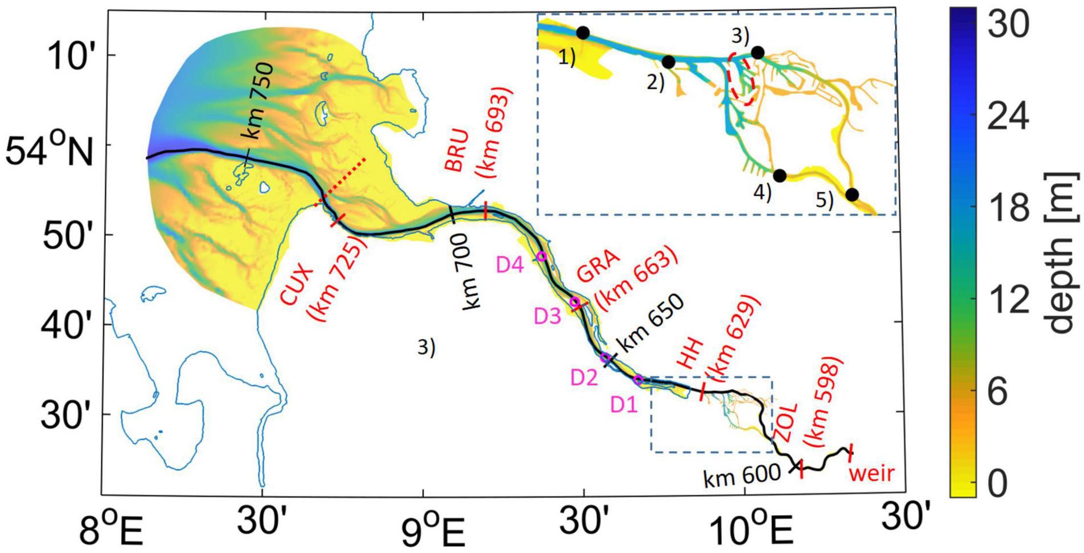
Figure 1. Model domain with depth [m] given as a background. The black transect line indicates the Elbe navigational channel, with black labels identifying the official Elbe-km. Red labels and associated ticks mark the locations of observation stations for (but not only) water quality parameters, with respective official Elbe-km given as additional information. Purple circles mark the locations of permanent moorings where horizontal currents, salinity, and temperature are measured, with purple labels D1–D4 identifying the individual stations. The inset in the upper right corner indicates the locations of gauges in the region of the port of Hamburg used for model validation: (1) Blankenese, (2) Seemannshöft (labeled “HH”), (3) Sankt Pauli, (4) Harburg, and (5) Bunthaus. The red dashed line marks a port basin subject to analysis in Figure 11.
Ecosystem Model
The ecosystem model is inherited from the ECOSystem MOdel (ECOSMO, Schrum et al., 2006; Daewel and Schrum, 2013), which originally had a hydrodynamic core of its own (Schrum and Backhaus, 1999). For this study, the ecological module of ECOSMO has been one-way coupled to the SCHISM via a messaging interface, the Framework for Aquatic Biogeochemical Models (Bruggeman and Bolding, 2014). ECOSMO has been developed to predict the lower trophic level ecosystem dynamics of the North Sea (Schrum et al., 2006) and the Baltic Sea (Daewel and Schrum, 2013). In the following we shortly describe the parts of the model that are either very relevant in the specific area of the study or that have been changed in comparison with Daewel and Schrum (2013).
For this study of a heterotrophic estuary, the organic matter decay, the coupled nitrogen and oxygen cycles and the exchange between the water column and the sedimentary layer are key processes for simulating the ecosystem dynamics. Organic decay starts when biological production has reached its final particulate stage, detritus. The source terms for detritus comprise faecal production by zooplankton, zooplankton mortality and phytoplankton mortality (see Figure 2 for the linkages between the ecosystem state variables). The sink terms comprise feeding by zooplankton and mineralisation. Particulate organic matter has a settling velocity w_d. At the bottom, it is deposited to the sedimentary layer given the bottom shear stress (τb) is below a value (τc = 0.3 N m–2). For τb≥τc, the sediment is re-suspended with the rate λs2d is estimated as:
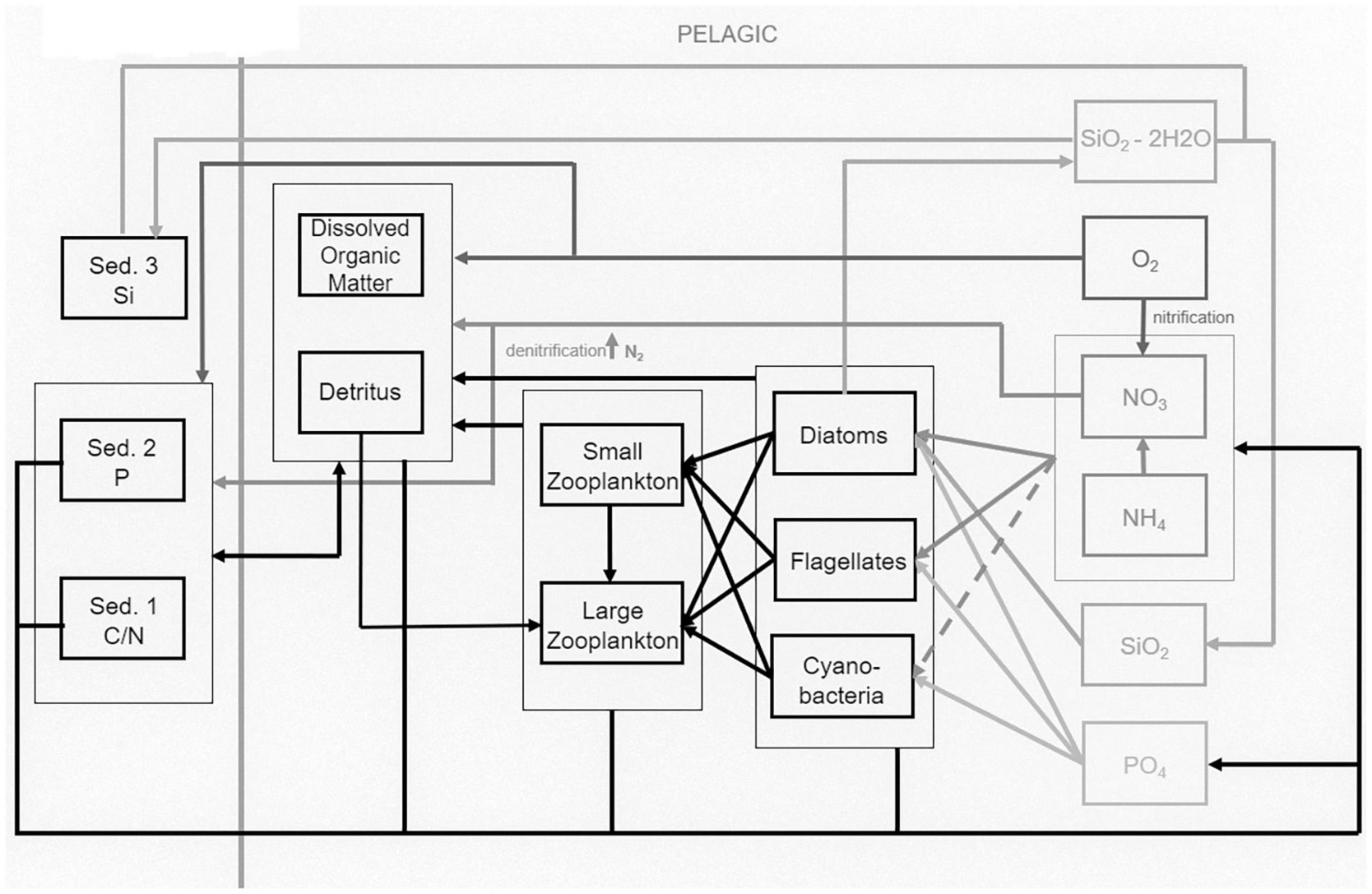
Figure 2. Links between the pelagic and benthic state variables in ECOSMO2 [figure adapted from Benkort et al. (2020)].
with constant M = 5 m d–1 herein. In the shallow coastal ocean and estuary dominated by tidal motion, organic matter (C, N) is regularly resuspended from the sedimentary layer to the water column. The mineralisation of organic matter depletes oxygen, while regenerating inorganic nitrogen (NH4) and phosphorus (PO4). The remineralisation rate is controlled by temperature and equals:
where Tref = 13°C is a reference temperature and k is a constant with k = 0.005d–1 in the water column and k = 0.003d–1 in the sediment layer.
Nitrification of ammonium to nitrate depends on the ambient water temperature and dissolved oxygen concentration (Stigebrandt and Wulff, 1987). The sources of ammonium include excretion by zooplankton and remineralisation of organic matter in the water column and in the sedimentary layer. Nitrification is the only autochthonous source of nitrate, while external sources are river loads and atmospheric deposition. Nitrate is taken up by primary producers and decreases due to denitrification under anoxic conditions. During denitrification nitrate is used as an oxidant in the remineralisation process and the remaining nitrogen leaves the system by outgassing. Denitrification depends on the local oxygen concentration and water temperature and occurs both in the water column and at the sediment interface.
Oxygen is an important indicator of estuarine water quality, reflecting the local relationship between production and respiration. The oxygen concentration increases due to the assimilation of nitrogen by phytoplankton and by air-sea exchange at the sea surface. The latter process is controlled by the saturation concentration of oxygen and the piston velocity vp (Liss and Merlivat, 1986). Respiration includes nitrification, grazing and mineralisation of organic matter. The latter depletes oxygen following the Redfield ratio of O:N = 6.25. Remineralisation, nitrification and denitrification occur in the water column and the sedimentary layer, whereas the sediment oxygen demand affects the lowermost pelagic grid cell (for details, see Daewel and Schrum, 2013). The list of the model state variables and the parameter table are given in Supplementary Tables 1, 2, respectively.
Model Forcing
At the open boundary, boundary conditions for the Elbe model are provided by the previously published German Bight model (Stanev et al., 2019). In turn, the latter receives sea surface elevation, horizontal currents, salinity and temperature at its boundary from the AMM7-based CMEMS reanalysis of the North-Western European shelf (O’Dea et al., 2017). For the marine biogeochemical forcing time series of nutrients, oxygen and organic matter from observations in the southern North Sea1 were prescribed at the open boundary. The available observations were averaged over the ICES area IVb excluding samples with salinities smaller than 34 psu to obtain a forcing representing marine variability. Those time series force the model in the area of a sponge layer extending from the open boundary into the model area. The thickness of the sponge layer is 15 km, and the relaxation constant decreases linearly from the outer boundary to the inner edge of the sponge layer.
At the landward end, river discharge enters the estuary, driving the downstream flow. The daily discharges are derived from observations at the tide-free gauge station at Neu Darchau, approximately 50 km upstream from the weir at Geesthacht. At this station the long-term average discharge is 710 m3 s–1, while standard deviation is 471 m3 s–1. During the period of model integration the yearly average discharges were 636 m3 s–1 in 2012 and 1012 m3 s–1 in 2013, and respective standard deviations were 373 m3 s–1 and 641 m3 s–1. Here, we calibrated the rating-curve-based discharge estimates to obtain permanent limnic conditions at measurement station D2 (Figure 1), adding 30% of the volume to the original time series. This correction seems necessary because the upstream gauge station does not account additional freshwater input from small tributaries and groundwater sources up to the tidal weir. For the inflowing volume, concentrations of nutrients, oxygen and organic matter are specified. The time series of concentrations were compiled from weekly to monthly measurements accomplished by the FGG Elbe and available via www.fgg-elbe.de/elbe-datenportal.html. The smaller tributaries, with an average discharge less than 20 m3 s–1, are represented as point sources at the location of the tributary mouth. These point sources contribute fresh water with ambient temperature and ambient nutrient concentrations at a rate equal to the long-term mean of the tributary’s discharge. A single exception is given by a point source representing the Hamburg sewage plant, which discharges 4.8 m3 s–1 with concentrations of organic and inorganic nitrogen derived from the annual environmental report of the plant in 2012. The atmospheric forcing includes wind, air temperature, precipitation, shortwave and longwave radiation and is based on reanalysis data generated by the COSMO-EU model of the German Weather Service (DWD). More details regarding the forcing at the air-sea interface are given in Stanev et al. (2019).
Observational Data
Elbe estuary data sources include observations from tide gauge stations and stationary long-term measurements of salinity, water temperature, horizontal currents, nutrients, oxygen, and chlorophyll concentrations. The tide gauge data and observations of surface and bottom currents, salinity and temperature are available via the data portal www.tide-elbe.de. For the period considered in this study (2012-2013), these data have a high temporal resolution between 1 min and 5 min and serve for calibration and validation purposes of the hydrodynamic simulation. Five out of six tide gauges considered herein are situated in the focal area of this study (see inset in the upper right corner of Figure 1), and one tide gauge represents the lower estuarine reaches (see label “BRU” in Figure 1). Temperature, salinity and current data were obtained from four permanent measuring stations (“Dauermessstationen,” see labels “D1,” “D2,” “D3,” and “D4” in Figure 1) located in the mid-estuarine reaches.
The long-term stationary observations of nutrients, oxygen concentrations and chlorophyll-a were collected at six locations along the Elbe estuary: at the weir at Geesthacht (km 585.9), Zollenspieker (km 598.7), Seemannshöft (km 628.8), Grauerort (km 660.5), Brunsbüttel (km 693.0) and Cuxhaven (km 725.2). In this study, the data from Geesthacht (see label “WGE” in Figure 1) are used for the riverine forcing. Observations from Seemannshöft and Grauerort (see labels “HH” and “GRA” in Figure 1) were used for model validation of the biogeochemical dynamics in the focal area. The measurements were taken by FGG Elbe as horizontal profile mixing probes or individual samples 1 h before low tide. Samples were taken, without lateral position information, approximately 1 m below the surface. Station data from 1979 – 2014 are available on a daily basis measured at weekly to monthly intervals, but there are different levels of data gaps depending on measurement station, parameter, season and year. For further model validation, stationary data were used comprising long-term nutrients and chlorophyll-a measurements taken by several local authorities and available through the websites www.gateway.hamburg.de and https://wiki.cen.uni-hamburg.de/ifm/ECOHAM/DATA_RIVER.
Statistical Evaluation Methods
For model validation, we use standard statistical measures and presentation methods, including the root mean square error (rmse), the Pearson correlation coefficient (R) and the Willmott skill score (WSS, Willmott, 1981). The rmse is given by the mean of the squared differences between predicted and observed realisations of a variable. This measure is useful as a straightforward quantitative assessment of the model simulation. Other than the rmse, R reflects how much the deviations of two signals from their respective means are alike during an interval in time. R is thus appropriate to quantify phase differences of oscillatory quantities in model and observations for example on tidal or seasonal time scales. High correlations between model and observations demonstrate good model representation of the underlying physical or biogeochemical processes. The WSS assesses the deviation of the simulated or predicted variability from the observed time series and reads as follows:
where n is the number of observations, O_i and P_i refer to a corresponding pair of observed and simulated values with index i and overbars denote the time average. The WSS offers a skill assessment that considers both the bias and the correlation between model predictions and observations. The value ranges between 1 (perfect agreement) and zero (no agreement).
For the graphical presentation of the agreement between model and observations regarding a single variable along the estuarine gradient or several variables at a single location, we use a Taylor diagram (Taylor, 2001). This measure locates the model performance regarding a specific variable in a specific location in a space spanned by the normalised standard deviation, normalised rmse, and the correlation coefficient, R. We use the Taylor diagram to illustrate the model performance either i) with respect to one (physical) variable along the estuarine density gradient or ii) regarding several different but interlinked (biogeochemical) variables at one position of the estuary. In this diagram, a perfect model simulation is indicated by a marker at the intersection of the X-axis and the circle with a radius of one standard deviation. Model deficiencies lead to scattering of the markers toward the regions of increased root mean squared error and reduced correlation coefficient, that is toward the tip of the Y-axis.
Results
Hydrodynamical Simulation Validation and Interpretation
The validation of the hydrodynamical model focuses on the freshwater-dominated reach of the Elbe estuary addressing vertical and horizontal tidal currents, salinity, water temperature, and stratification. In the following we show the essential aspects of the validation, while additional information are given in the Supplementary Material.
The tidal currents in the navigational channel are monitored by four moorings between km 677 and km 641 (Figure 3, for stations locations see Figure 1). At the surface, at station D3 (km 665), both flood and ebb currents attain approximately 1.5 m s–1 during peak flows demonstrating roughly symmetry (Figure 3A). The bottom currents reach 2/3 of the magnitude of surface currents, thereby demonstrating a pronounced vertical shear of the horizontal flows in the estuarine main channel (Figure 3B). At the upstream station D1 (km 643) flood-directed surface peak currents have magnitudes similar to the ones at D1 (Figure 3C), while maximum ebb currents reach 1 m s–1 only. The observed bottom currents are again weaker with peak flood currents twice as strong as ebb currents (Figure 3D). At D1, about 20 km downstream of the central port region, horizontal tides are thus clearly flood-dominant. This implies that in this area suspended particulates are subject to tidal pumping toward the port due to correlations between horizontal currents and suspended particle concentrations. The model replicates above characteristics of the tidal currents at D3 and D1, as well as the change between D3 and D1 (Figure 3). Simulated flood currents also quantitatively match well with the observations with the rmse calculating to 0.23 m s–1 (surface) and 0.17 m s–1 (bottom) at D3, and 0.28 m s–1 (surface) and 0.21 m s–1 (bottom) at D1. The model tends to underestimate currents at low water slack at D3 and late ebb currents at D1. Further, the model reproduces the propagation of the tidal wave from the lower reaches into the port area. For the period of 2012, the rmse calculates to 0.28 m at Brunsbüttel station and between 0.31 m to 0.35 m at the gauges located in the port area (Table 1, for gauge positions see Figure 1). The correlation coefficient, R, and the WSS are above 0.96 and 0.98, respectively. A comparison of the observed and simulated tidal water level variations is given in the Supplementary Material.
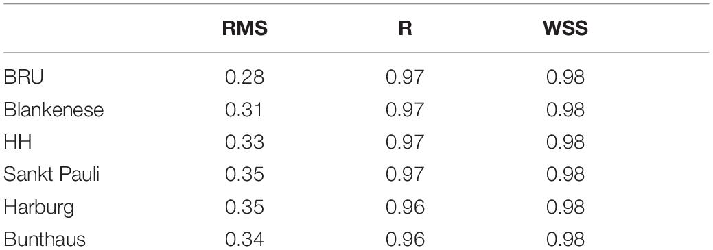
Table 1. Error statics of simulated sea level elevation compared against observations at six gauges in the Elbe estuary.
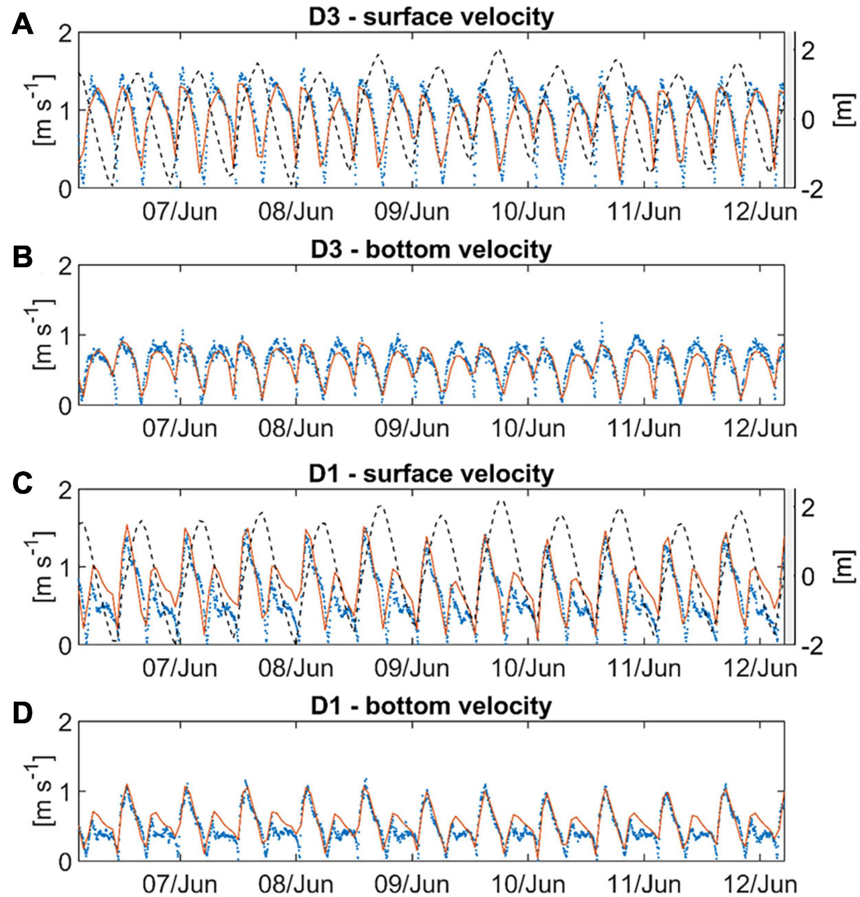
Figure 3. Comparison of the simulated (red solid lines) against the observed (blue dots) (A,C) surface velocity magnitude and (B,D) bottom velocity magnitude at the measurement stations (A,B) D3 and (C,D) D1 during the period from 6 June to 12 June 2012. The dashed line in (A,C) shows the local water elevation.
Simulated surface salinity is also in good agreement with observations along the main channel and Supplementary Figure 2 illustrates the model performance by means of a Taylor diagram. For realistic simulation of density gradients and ecosystem dynamics in the freshwater-dominated reach good model performance of simulated temperature is important. A Taylor diagram of the model error statics compared to observations for the surface temperature reveals high correlations of approximately 0.99 and small relative errors of approximately 0.2°C (Figure 4A). The stations used for model-data comparison cover the main channel between the deep lower estuary and the shallow area upstream from the port (Figure 4B). The average (for the period of May to September 2012) surface temperatures at these stations are instructive because they show a mild gradient over the mid reaches but a steepening gradient toward the shallow upper estuary. Given these horizontal temperature gradients, the vertically sheared horizontal currents induce vertical density gradients if i) temperature controls the equation of state, and ii) turbulent mixing does not cancel out the vertical gradients.
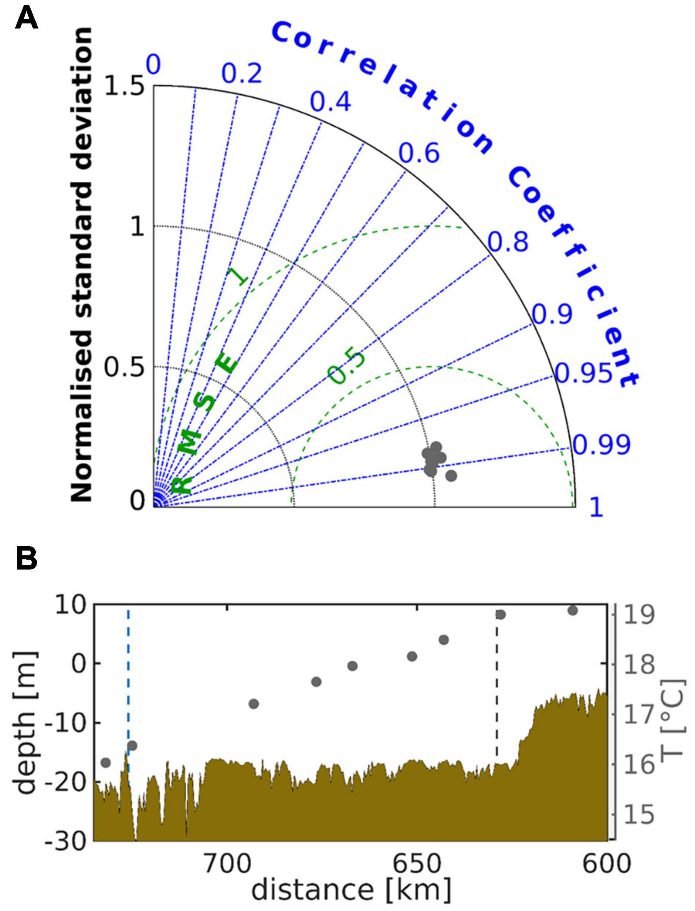
Figure 4. Taylor diagram representing the normalised standard deviation, the correlation coefficient, and the root mean squared error of (A) simulated surface temperature against respective observations at several stations along the main estuarine channel. In (A), the grey dots represent locations between km 725 and km 609. In (B) the shaded area illustrates the along-channel depth distribution and the grey dots represent the observed near-shore surface water temperature between May and September 2012. The black and blue dashed lines mark the stations Seemannshöft and Cuxhaven, respectively; see labels “HH” and “CUX” in Figure 1.
A comparison of observed and simulated density variability for the time of model integration (2012–2013) at the stations D1-D4 (Figure 1) is given in the Supplementary Figure 3. Both model and observations reveal permanently fresh (limnic) conditions at D1 (km 643) and D2 (km 651), oligohaline conditions at D4 (km 677). At D3 (km 665), observations indicate a permanent freshwater dominance, while the model shows an oligohaline regime in summer. Observations from stations D1-D4 also allow for the estimation of the bulk stratification in this part of the estuary. A bulk Richardson number is commonly used to characterise the stability of a stratified flow (for example, Tedford et al., 2009):
where g is the gravitational acceleration, H is the total water depth, Δρ is the density difference between the bottom and surface, Δu is the velocity difference between the surface and bottom and ρ0 is a reference density. The resulting estimated time averages (median values) of Ri_B at stations D1-D4 are D1: 6.10 (0.23), D2: 3.67 (0.09), D3: 2.63 (0.09), and D4: 3.52 (0.09). The median values provide an idea of the distribution of local mixing conditions in time. At the lower stations D2, D3, and D4, half of the observations manifest well-mixed conditions, with RiB = 0.09, which is well below Ricrit = 0.25. At station D1, the median value represents mixing conditions near the critical condition, implying periodic stratification of the water column. Given the flood-dominant conditions at D1 the water column stratifies on ebb whereas the strong flood currents lead to complete vertical mixing.
For a spatially better-resolved assessment of the stratification, we use simulated horizontal currents and density to calculate the gradient Richardson number (Ri):
where z is the vertical coordinate. Similar to the bulk estimates derived from the observations, model-derived Ri above the well-mixed bottom layer is low near D2 (km 665, left-hand end of Figure 5A) and increases in upstream direction. At D1 Ri has a local maximum beyond which the measure remains elevated, while falling to background levels over the shallow upper estuary (Figure 5A). Particularly the area of the bathymetric jump between km 623 (green dashed line) and km 618 (channel depth ∼ 5 m) indicates stable flow conditions. The dynamical picture is further clarified by comparing the ratio of the turbulent diffusivity during flood and ebb (Figure 5B). In this figure, warm colours identify flood-dominated mixing and cold colours represent ebb-dominated mixing, while times of flood (ebb) are defined as times of locally rising (falling) tide. In agreement with the above shown dominance of the flood currents (Figure 3), the ratio is greater than unity in the deepened part of the channel (until km 620, Figure 5B). Upstream from the bathymetric jump the ratio is smaller than unity. This indicates that turbulent exchange (mixing) is flood-dominated in the deepened part and ebb-dominated over the shallow part. Dissolved properties and particulates are thus mixed up high in the water column differentially and the zone of convergence is exactly the bathymetric jump. This is an important result of the hydrodynamic simulation because it explains the accumulation of particulates (sediment and biogenic particles) in the port area (see Kerner, 2007). The flood-dominance of the turbulent diffusivity over the deep channel also implicates that the elevated values of Ri (Figure 5A) are due to stratification of the water column during ebb. Figure 5B represents the conditions along the transect line passing through the northern branch of Elbe river in the port area (Figure 1). Ri and the ratio of flood to ebb mixing are also given for a transect following the southern branch in the Supplementary Figure 4 emphasising the robustness of the results. The time-averaged vertical temperature anomalies reveal systematic surface-bottom difference downstream from the bathymetric jump (Figure 5C). In the freshwater-dominated reach temperature-induced density differences account for stratification of the water column during ebb (Figures 5A,C). The mixing asymmetry finally leads to systematic vertical shears of the average longitudinal currents with enhanced seaward flow near surface and recirculation near the bottom (see black arrows in Figure 5C). Given the overall consistency of the hydrodynamic simulation with the available observations and derived measures of stratification, the hydrodynamic simulation of the Elbe presented herein is approved as a credible tool to explore the 3D coupled physical-biological dynamics.
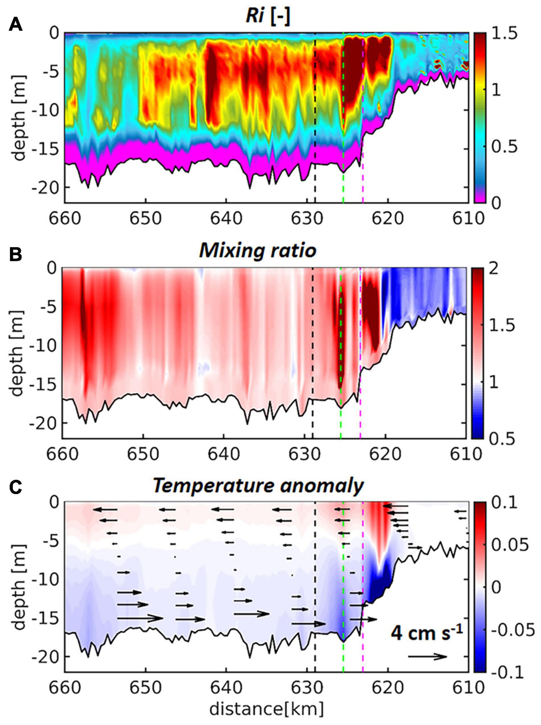
Figure 5. Time-averaged along-channel profiles of simulated (A) Gradient Richardson Number, (B) ratio of flood diffusivity to ebb diffusivity (mixing asymmetry), (C) vertical temperature anomaly, are given for the period May to September 2012. In (C) black arrows represent the local deviation of the along-channel velocity from the barotropic along-channel velocity. The black dashed line marks the Seemannshöft station (see label “HH” in Figure 1), whereas green and purple dashed lines indicate the positions of the confluence of northern and southern channel branches and Sankt Pauli gauge station, respectively (see inset in Figure 1).
Validation of Biogeochemistry
The validation of the ecosystem model focuses on the port area. The locally most relevant measuring station is located at km 629 (see location labelled “HH” in Figure 1), approximately 3.5 km downstream from the convergence of the northern and southern channel branches. At this station nitrate, silicate and oxygen concentrations are characterised by a clear seasonal signal with high winter and low summer levels (Figures 6A,C,D), whereas chlorophyll demonstrates the opposite pattern particularly with respect to the silicate dynamics (Figure 6E). Ammonium levels reach maxima during summer and autumn, whereas winter concentrations mostly fall between 5 and 10 mmol m–3 (Figure 6B). The time series is somewhat scattered, with fluctuations in the range of the seasonal variability occurring within a time span of a month, for example, in June 2012. The simulated time series at the same location convey a smoother picture of the nutrient and oxygen variability, emphasising the seasonality of respective signals with the exception of ammonium (Figure 6). The simulated nitrate, silicate and oxygen levels match the seasonal extremes very well (Figures 6A,C,D) with the WSS calculating to 0.95, 0.98 and 0.93, respectively. In the case of ammonium, the model predicts a short-term variability similar to that of the observations, which manifest higher amplitudes of the small-scale variability and imminent scatter (Figure 6B). In addition, the observed levels rarely fall below 5 mmol m–3, while the simulated ammonium concentrations approach zero over a period of up to several weeks, particularly during the cold season. The resulting systematic bias between the observed and simulated signals is more pronounced in 2012 than in 2013. The second run year manifests 54% higher average river discharge (not shown) and consequently enhanced flushing rates that tend to reduce the influence of local processes or sources. The peak ammonium concentrations and low oxygen levels during the summer months are manifested in both observations and simulations. The along-channel transition from production to consumption is reflected by the comparison of chlorophyll observations at the upstream station Zollenspieker (Figure 6E, see label “ZOL” in Figure 1 for the location) with those at the downstream station Seemannshöft (Figure 6F, see label “HH” in Figure 1 for the location). The upstream station is situated at the channel bifurcation and captures a clear seasonality with summer chlorophyll levels between 100 and 250 mg m–3 in 2012 (Figure 6E). At a distance of 31 km further downstream, the summer levels decrease considerably, reaching approximately 50 mg m–3 (Figure 6F). The model simulation captures the seasonal dynamics in and the systematic difference between both stations (Figures 6E,F). The model tends to underestimate the spring bloom at the upstream station and overestimate the spring bloom at the downstream station. In general, the model simulations reproduce the fundamental aspects of the Elbe ecosystem associated with the remineralisation processes in the port area. A Taylor diagram based on the time series shown in Figure 6 provides a condensed assessment of the model performance in the port area (Figure 7A). In this figure, the state variables with strong seasonality are associated with high correlation between model and data and low normalised model error. This applies to silicate, nitrate and oxygen. The simulation attains significant correlation with observations regarding chlorophyll-a and ammonium. At the downstream station Grauerort (see label “GRA” in Figure 1 for the location), the model adequately simulates oxygen and the macronutrients of nitrate and silicate with a high correlation and small relative error (Figure 7B). The correlation of ammonium is weak, but the relative error is small. Additional statistics of the model performance regarding nitrate, oxygen and silicate emphasise the quality of the ecosystem model simulation (Supplementary Table 3 given for five stations along the estuarine main stem).
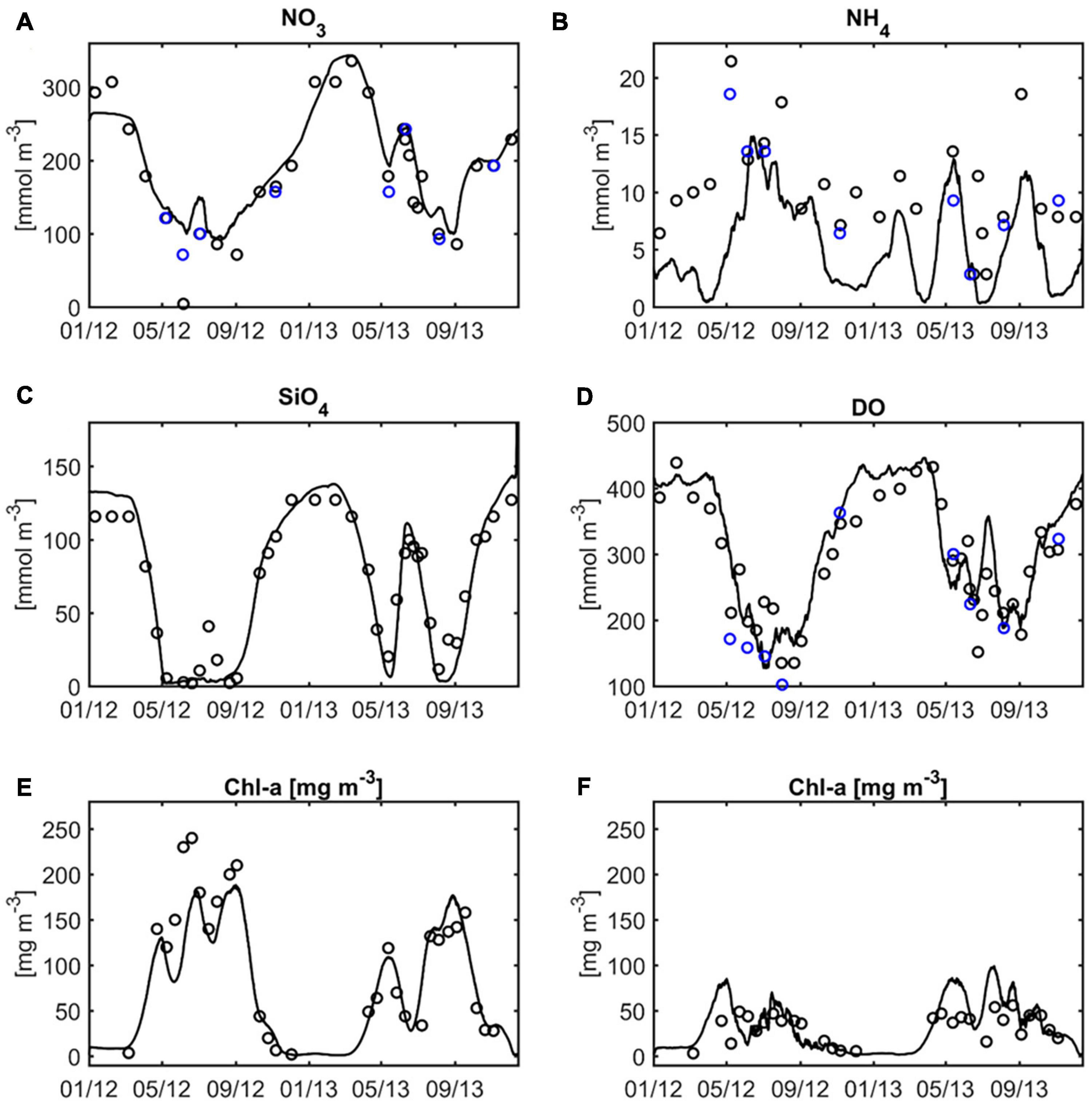
Figure 6. Comparison of simulated and observed surface concentrations of (A) nitrate, (B) ammonium, (C) silicate, and (D) dissolved oxygen Seemannshöft station (see label “HH” in Figure 1). The bottom panels show the simulated and observed surface concentrations of chlorophyll-a at (E) Zollenspieker station (see label “ZOL” in Figure 1) and (F) Seemannshöft station. Blue circles in (A,B,E) represent additional observations provided by the Institute of Oceanography (IFM), University of Hamburg.
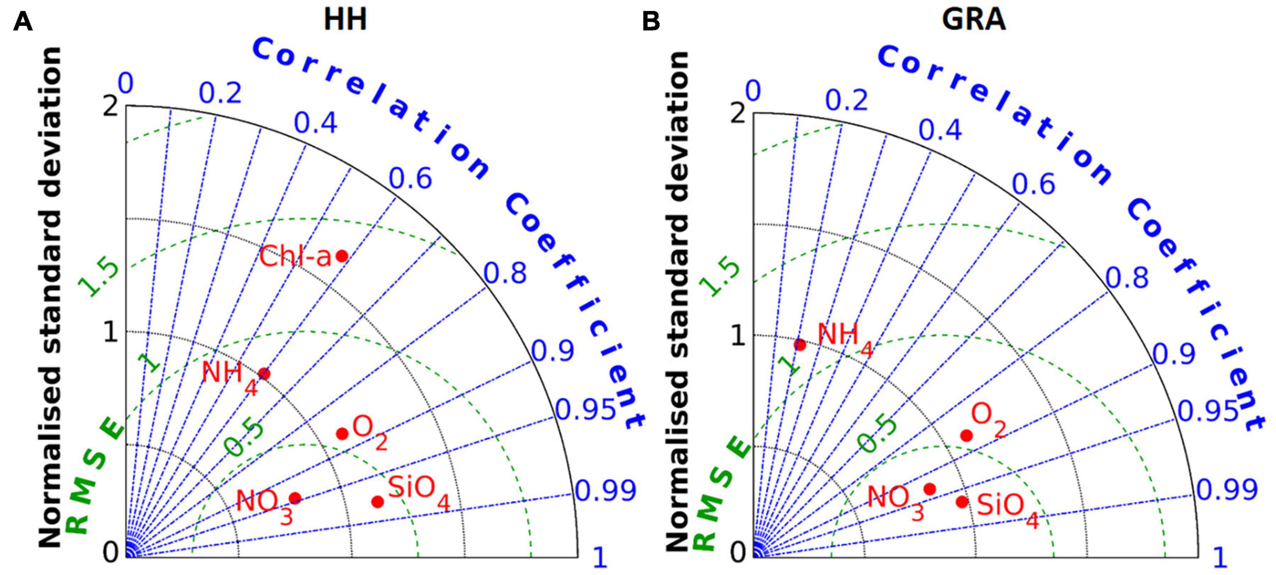
Figure 7. (A,B) Taylor diagrams illustrate the model performance regarding nutrients and oxygen at the stations of Seemannshöft (HH) and Grauerort (GRA). Chlorophyll measurements were available only for Seemanshöft and are represented in (A).
Biogeochemical Gradients in the Main Channel
The estuarine ecosystem dynamics are dominated by inputs of allochthonous phytoplankton and nutrient loads at the tidal weir (km 585). The variability of these inputs determines the pace of the processes inside the estuary. A detailed description of the seasonal variability of the dominant primary producers, grazers, oxygen and nutrients between the weir and the lower end of the port area is provided in the Supplementary Material. In the following, we present the longitudinal structure of the main channel ecosystem dynamics during the productive period that frame the physical-ecological interactions in the port area. The along-channel summer average profiles of the state variables primarily involved in the organic to inorganic transformation and respiration illustrate the along-channel vertical structure of the estuarine reactor (Figure 8). The longitudinal sequence of the transition of organic matter to the inorganic pool is evident from the order of estuarine maxima of chlorophyll, with its maximum at the tidal weir (Figure 8A), followed by particulate organic matter (detritus) peaking in the port area (Figure 8B) and ammonium peaking in the port area with levels gradually decreasing downstream (Figure 8D). Downstream from the detritus and ammonium maxima, oxygen reaches its estuarine minimum, developing a clearly delineated OMZ between km 650 and the port area (black dashed line in Figure 8C indicating the location of station Seemannshöft). The silicate concentration levels have an estuarine minimum at the downstream end of the shallow upper estuary (Figure 8E). The decrease in silicate reflects the growth of diatoms in the shallow reach, suggesting that the silicate levels exert a certain control on the oxygen and, consequently, on the nitrogen cycle in this area. Both silicate and nitrate are regenerated downstream from the port area (Figures 8E,F). The nitrate concentration levels reveal clear along-channel gradients around their estuarine maximum at km 670. The longitudinal gradients develop into vertical gradients due to differential advection in the near-surface region. Specific mechanisms contribute to the stratification of detritus and dissolved oxygen (Figures 8B,C). The former is a sinking tracer accumulating, per definition, near the bottom (see the area near the port measurement station marked by the black dashed line in Figure 8B). Oxygen shows depletion toward the bottom, particularly in the area of the OMZ, due to the demands from detritus and deposited sediments, whereas reoxygenation at the air-water interface increases oxygen concentration in the upper water column.
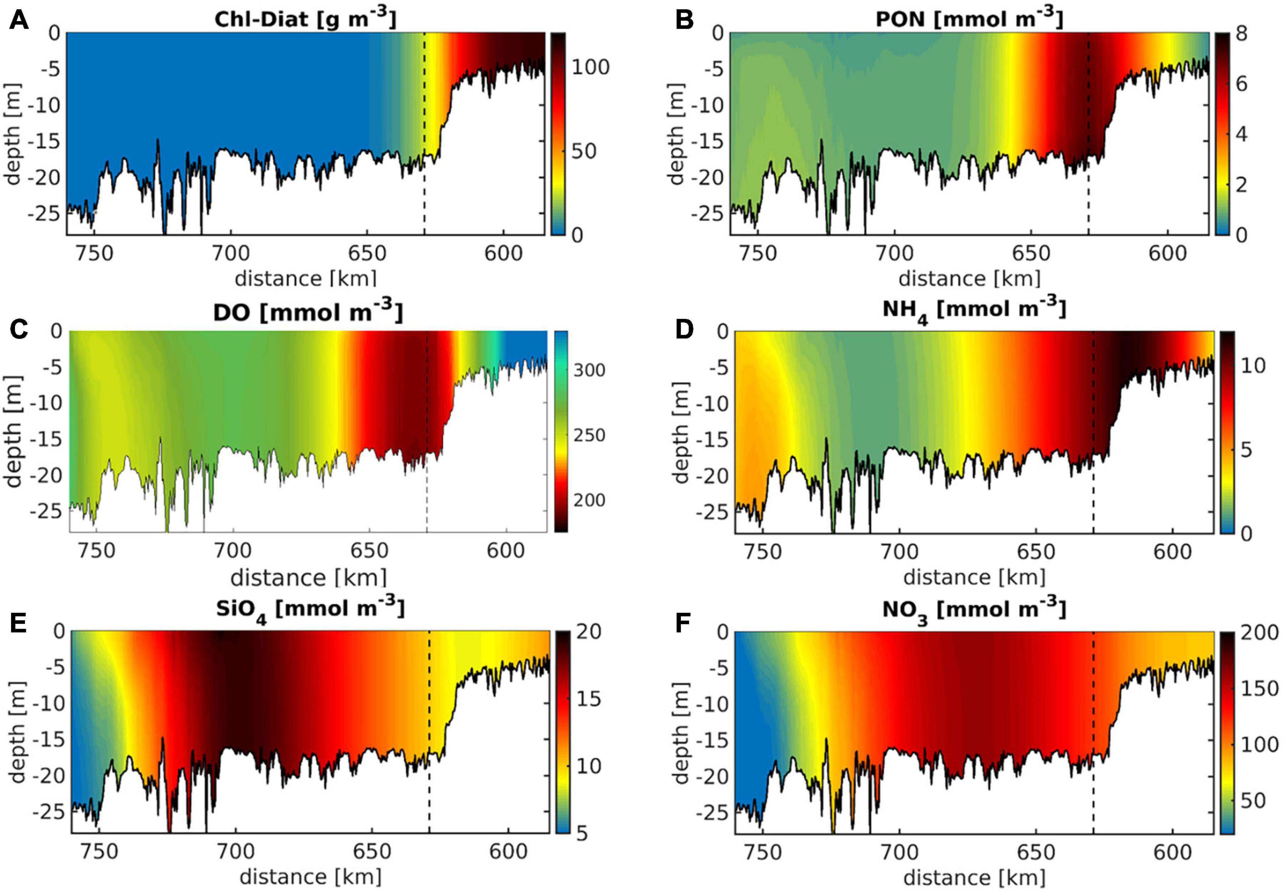
Figure 8. Time-averaged vertical anomalies of (A) chlorophyll, (B) detritus, (C) dissolved oxygen, (D) ammonium, (E) silicate, and (F) nitrate concentrations are given for the main channel between km 610 and km 640 of the Elbe estuary. The time averages represent the simulation during the period of May to September 2012. Note different colour bar in (C) with warm colours representing low oxygen levels.
Biogeochemical Dynamics and Stratification in the Port Area
Zooming into the port area, most of the state variables shown in Figure 8 reveal surface-to-bottom differences in the area of the bathymetric jump and downstream in an illustration of the along-channel vertical anomalies (Figure 9). Chlorophyll, silicate and nitrate demonstrate vertical anomaly pattern very similar to the one of water temperature (Figures 9A,E,F vs. Figure 5C) with silicate and nitrate increasing toward the bottom. Detritus and dissolved oxygen show significant vertical gradients with a surface-bottom difference in the range of 5–10 % of the local absolute concentrations (Figures 9B,C vs. Figures 8B,C). The vertical anomalies of ammonium (Figure 9D) are relatively small and the associated patterns appear less systematic in comparison with the other state variable. This illustration of the vertical gradients of some key ecosystem state variables highlights the tendency of the ecological compartment to amplify even subtle physical gradients. These along-channel and vertical gradients emerging at the interface between the shallow upper estuary and the deepened freshwater reach are intensified by the manifold side channels and basins of the port area (see inset zooming into the port area in Figure 1).
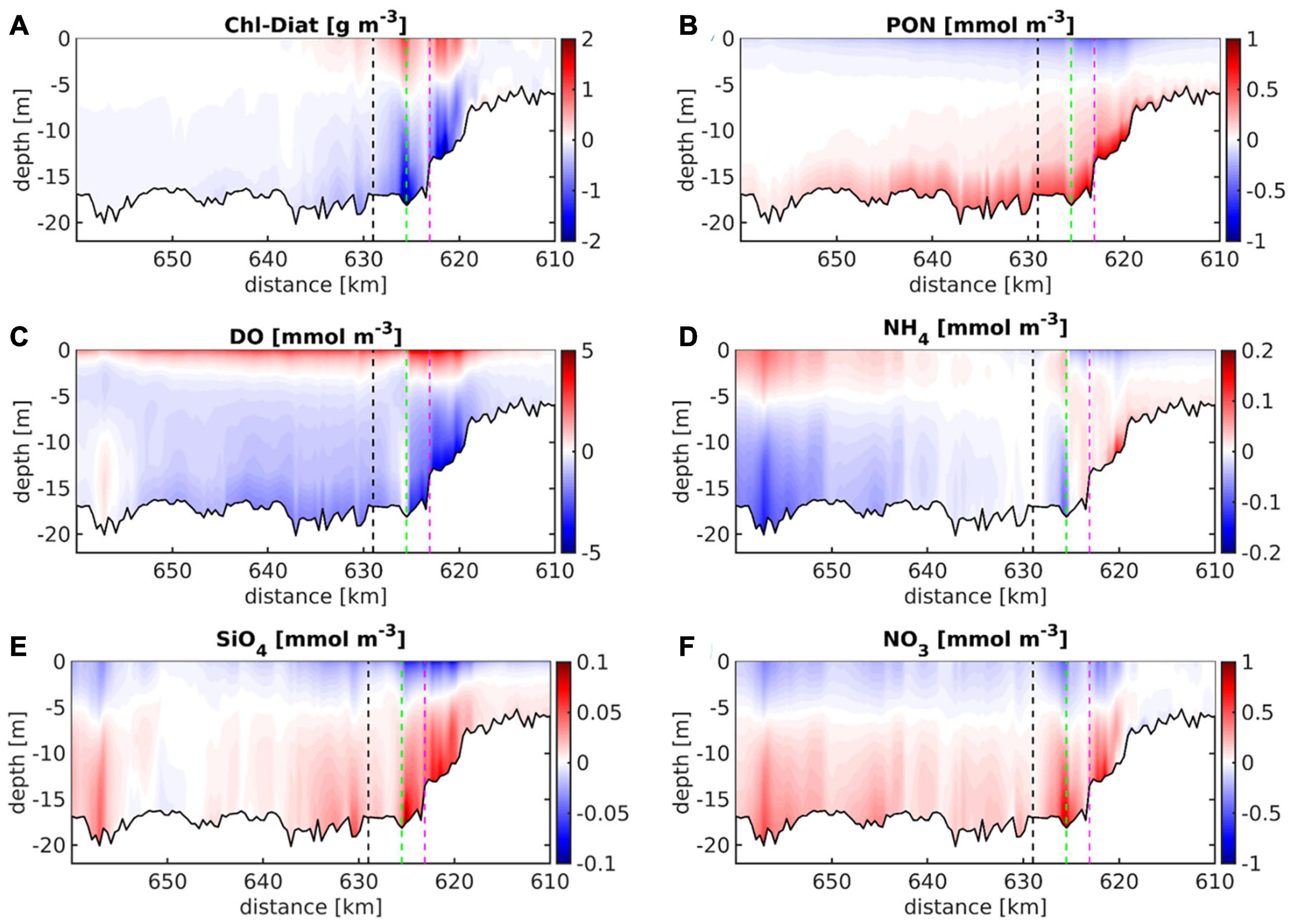
Figure 9. Time-averaged vertical anomalies of (A) chlorophyll, (B) detritus, (C) dissolved oxygen, (D) ammonium, (E) silicate, and (F) nitrate concentrations are given for the main channel between km 610 and km 640 of the Elbe estuary. The time averages represent the simulation during the period of May to September 2012. The dashed black, green, and purple lines mark the positions of station Seemannshöft (“HH,” see Figure 1), the confluence of the northern and southern channel branches, and station Sankt Pauli (see inset in Figure 1), respectively.
In the port basins, primary producer concentrations generally decrease toward the inside of the basins (Figure 10A), whereas the grazer concentrations increase in the same direction. In the port basins, enhanced secondary production leads to locally high accumulation of organic sediment (Figure 10D), whereas in the adjacent main channel biogenic particles remain suspended as detritus (Figure 10C). The port basins function as hotspots of the remineralisation processes, displaying increased ammonium concentration levels and local bottom oxygen depletion (Figures 10E,F). The resuspension of bottom sediments and dispersion of detritus along the deepened limnic reach leads to the formation of an “organic” high turbidity zone between station D1 and the port area (Figure 10C). The dispersion of the dead organic material and subsequent remineralisation to ammonium is reflected by the elevated ammonium concentration levels in the same region and, in particular, that over the shoals (Figure 10E).
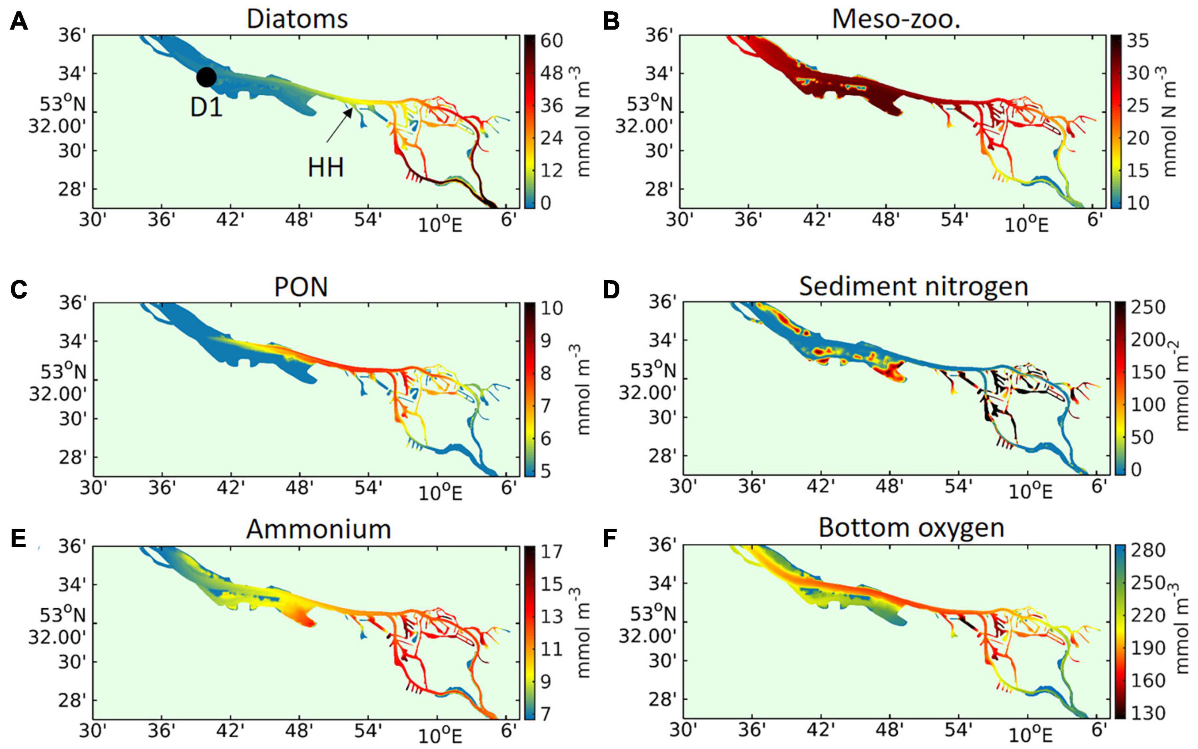
Figure 10. Model-simulated vertically averaged and time-averaged concentrations of (A) diatom biomass nitrogen, (B) meso-zooplankton biomass nitrogen, (C) particulate organic matter, and (E) ammonium in the area of the port of Hamburg. In (D,F) the model-simulated time-averaged (D) mass per square meter of sediment nitrogen and (F) near-bottom dissolved oxygen concentration are given for the same area and period of May to September 2012. In (A) the locations of two measuring stations are marked by a black dot (station “D1,” see Figure 1) and by a black arrow (stations Seemannshöft, see label “HH” in Figure 1).
The time series of ammonium, nitrate, diatom, and zooplankton biomass and oxygen concentration illustrate the seasonal variability of the coupled nitrogen and oxygen cycles in a major port basin (Figures 11A,B). The location marks a pronounced spring bloom that is followed by the growth of grazers and an increase in the ammonium concentration levels (Figure 11B vs. Figure 11A). During summer, diatom biomass remains below the spring bloom level. The similarity of the port basin time series of diatom biomass nitrogen with the time series of diatom chlorophyll recorded in the main channel (Figure 11B vs. Supplementary Figure 5A) and the spatial diatom distribution of diatom nitrogen given in Figure 10A suggest that during summer, diatoms are advected from the main channel into the port basins. Zooplankton, on the other hand, appear to be of autochthonous origin (not primarily advected) because the spatial maxima in the port basins and that in the main channel are separated (Figure 10B). The advection between the port basin and the main channel, the average Richardson number and concentrations of major ecological variables are shown in the Supplementary Figure 6. In the port basins, grazer biomass attains comparable levels as that of the diatoms (Figures 10A,B, 11B), indicating that they take up most of the biomass contained in the primary producers plus additional biomass advected to the basin (see also Supplementary Figure 6). Zooplankton mortality and grazing then lead to the production of detritus that functions as labile particulate organic matter. Accordingly, detritus (brownish solid line in Figure 11A) loosely follows the temporal development of diatoms, suggesting a rather indirect relationship between the two variables. In Figure 10C, the dead organic material reveals a homogeneous zone of elevated concentrations in the area of the central port basins and the confluence of the river branches, suggesting that the port basins receive detritus from the major channels.
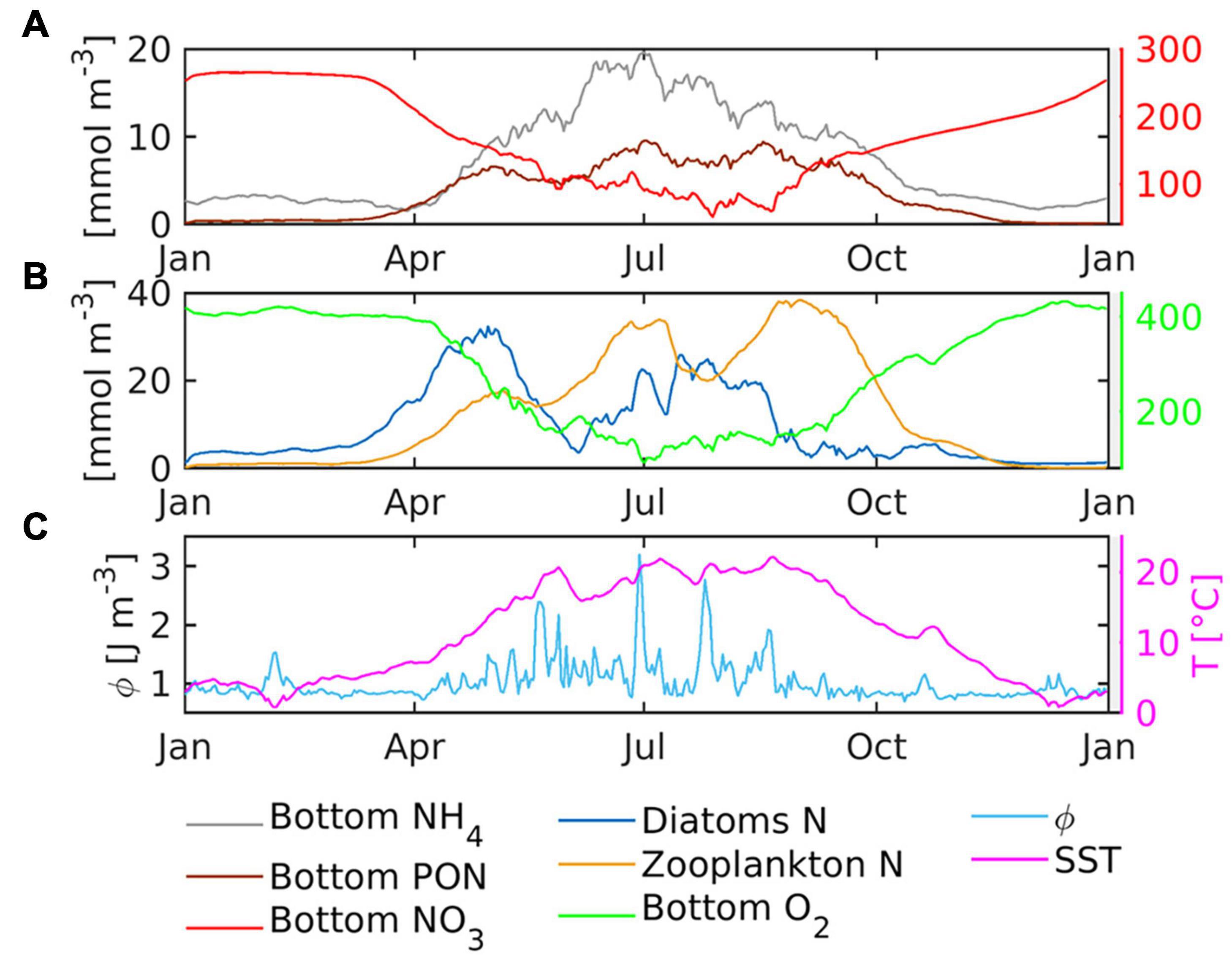
Figure 11. Time series of daily near-bottom (A) ammonium, detritus (PON) and nitrate concentrations, (B) vertically averaged diatoms and zooplankton concentrations and near-bottom concentration of oxygen, (C) daily potential energy anomaly (Φ) and sea surface temperature in a major port basin where all time-series represent the spatial average for local depth h > 10m. The location of the port basin is marked by the red dashed line in the top inset in Figure 1.
Impact of Stratification on Biogeochemistry
The accumulation of organic matter in the port area due to tidal pumping could be further intensified by baroclinic processes associated with the relatively weak ebb currents and steepening longitudinal temperature (density) gradients at the interface between the shallow upper estuary and the deepened freshwater reach. The environment created by the bathymetric jump is similar to the sloping region between the shelf and the deep ocean or the river mouth and the shelf sea where often plume-effects occur. In shallow, tidally dominated systems periodic stratification is typically generated by tidal straining. An appropriate measure to estimate the straining-induced stratification is given by the potential energy anomaly (Simpson, 1981):
where η is the local water elevation and D = H + η. Figure 12A illustrates the average distribution of Φ in the limnic reaches of the Elbe estuary, including the port basins, during the period of May to September 2012. In the shallow tidal river and over the shoals, stratification Φ is (near) zero, demonstrating locally well-mixed conditions (Figure 12A, inset showing port bathymetry in Figure 1). In deepened channel parts, Φ clearly exceeds zero (Figures 12A, 11C), approaching unity in the western part of the port area, the southern branch of the bifurcated channel and downstream from the port toward station D1. The deepened limnic reaches of the Elbe estuary thus demonstrate average conditions indicative of stable stratification, supporting the hypothesis of strain-induced stratification and associated two-layer flow.
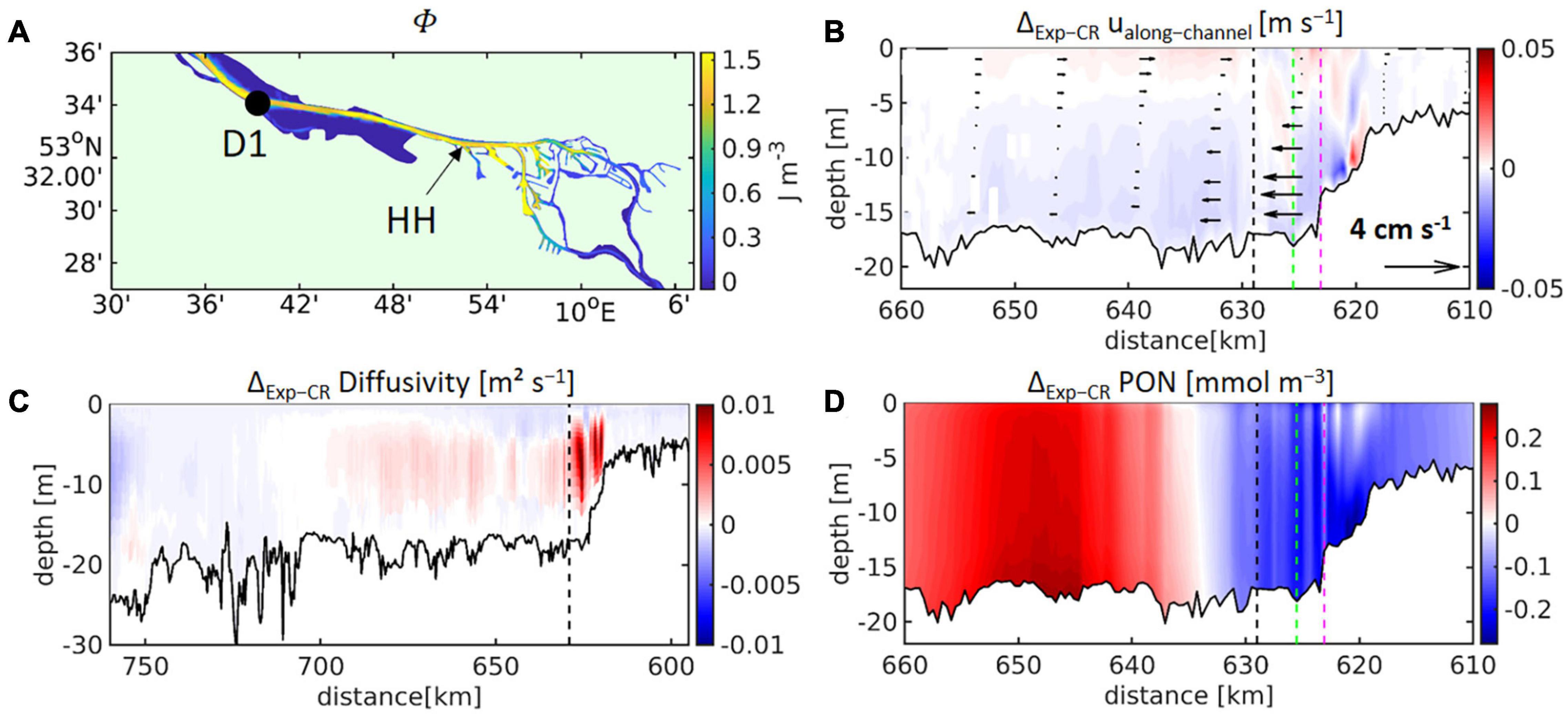
Figure 12. (A) The vertically averaged and time-averaged potential energy anomaly (Φ) is given for the focal region of the study, whereas (B) represents the along-channel profile of time-averaged differences experiment-control run (Exp–CR) of the vertical eddy diffusivity. Zooming into the deepened freshwater reach, (C) illustrates the time-averaged differences experiment-control run of the along-channel velocity and (D) represents the time-averaged differences of the detritus/particulate organic nitrogen (PON) concentration. The time-averages cover the period May to September, 2012. The black dashed line in (B–D) marks the station “HH” (see Figure 1), whereas green and purple dashed line in (B,D) indicate the confluence of northern and southern channel branches and gauge St. Pauli, respectively.
In the freshwater regime, density gradients are necessarily temperature-driven. Therefore, to test our hypothesis, an additional model experiment excluding temperature-induced density stratification is added to the study. For this purpose, the temperature was set constant in the equation of state in the model code (i.e., ρ=ρ(S,Tconstant,p) instead of=ρ(S,T,p), where T and p refer to temperature and pressure, respectively, and Tconstant = 14°C) and the model simulation was repeated. This additional model experiment with constant water temperature in the term stipulating water density (from now on “Exp-T14”) was compared to the control run (CR) (Figures 12, 13). Figure 12C shows the time-averaged differences in vertical eddy diffusivity for the period of May to September 2012. Red colours in Figure 12C represent increased eddy diffusivity in Exp-T14 in relation to that in CR. This figure demonstrates that eliminating the influence of temperature on water density leads to increased mixing over the bathymetric jump and the deepened limnic reaches (km 620 to km 690 in Figure 12C). The increase in mixing is higher for the ebb phase of the tidal cycle (for a tidally resolved representation of changes to near-bottom turbulent kinetic energy, see Supplementary Figure 7), thereby reducing the flood-positive asymmetry of the tidal mixing. Consequently, the along-channel residual flows are slightly changed in the opposite direction of the estuarine circulation (Figure 12B). The modifications to the tidal mixing asymmetry and the residual circulation impact directly on the along-channel distribution of the particulate organic material (Figure 12D). The detritus concentrations decrease in the area of the bathymetric jump and increase about 30 km downstream at the lower end of the OMZ (Figures 12D, 13A).
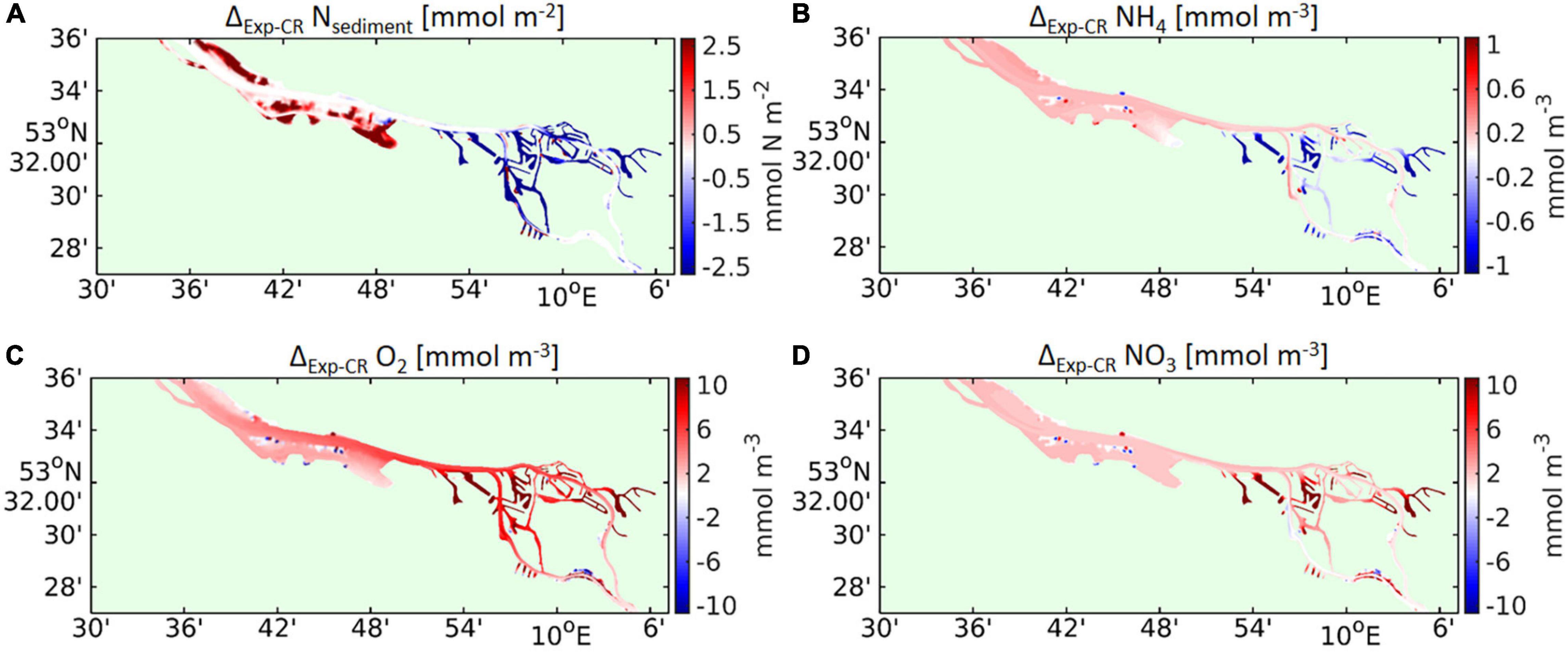
Figure 13. Spatial maps represent the time-averaged differences between the experiment and the control run (Exp–CR) of (A) mass per square meter of sediment nitrogen and concentrations of (B) near-bottom ammonium, (C) near-bottom oxygen, (D) near-bottom nitrate whereas near-bottom refers to the lowermost pelagic cell and time-averages represent the period May to September 2012.
The numerical experiment also manifests systematic impacts of the temperature-induced stratification on the non-sinking biogeochemical variables (but that are linked to detritus via kinetic reactions, Figure 2). Time-averaged differences in the organic sediment mass have a negative sign throughout the port area, while the organic sediment increases in the downstream main channel (Figure 13A). The elimination of temperature-induced density gradients thus shifts organic sediments from the port area toward the mid-estuarine reach, implying that in realistic cases, temperature gradients reduce the chances of particulate material leaving the port region. The displacement of bottom sediment in the numerical experiment reduces the near-bottom ammonium concentrations in those areas where resuspension of sediment is unlikely and ammonium is replenished primarily from sediment remineralisation (Figure 13B). This pattern clearly applies to the port basins (regions in blue colours in Figure 13B), which are protected from strong tidal currents. The main channel shows elevated ammonium concentrations in the Exp-T14 simulation in comparison with the CR, suggesting that the increased turbulence (Figure 12C) keeps the dead organic material suspended, allowing for a higher remineralisation rate. The improved vertical exchange has the strongest impact on the near-bottom oxygen concentrations, which increase by as much as 10 mmol m–3 in the port basins and by approximately 7 mmol m–3 in the main channel downstream of the port region (Figure 13C). Increased oxygen levels allow for accelerated nitrification and reduce denitrification, leading to enhanced nitrate levels, particularly in the areas with improved oxygen availability (Figure 13D). Similar to the case of oxygen, nitrate levels increase by approximately 10% in comparison to those in the CR. The experiment highlights the coupling of physics and biochemistry in the freshwater reach of the Elbe estuary and, in particular, the coupling between the oxygen and nitrogen cycles in the port area. Alternatively, the relationship of temperature-induced stratification and biogeochemistry can be tracked by correlating the temporal change in stratification and the temporal change in biological state variables. Although this approach might fail due to a time lag between the causal signal (stratification) and the response (biogeochemistry), Supplementary Figure 8 demonstrates systematic patterns of the correlation coefficients of stratification-diatoms, stratification-mesozooplankton, stratification-ammonium, stratification-nitrate, stratification-oxygen, and stratification-sediment. An increase in the potential energy anomaly is associated with an increase in the sediment and ammonium concentrations, while oxygen tends to be depleted. This pattern applies clearly to the port region, while in the downstream limnic main channel (around station “D1”), increasing stratification correlates with increasing oxygen levels and decreasing ammonium concentrations. In this area, stratification promotes estuarine circulation such that enhanced near-bottom upstream flows tend to shift high-oxygen and low-ammonium water from the mid-estuarine reaches toward the port region.
Discussion
Comparison of the Results With Other Studies
The 3D coupled model simulations reproduced the along-channel patterns of ecosystem dynamics known from idealised modelling studies of the Elbe estuary (Schroeder, 1997; Geerts et al., 2017; Holzwarth and Wirtz, 2018). The previous studies did not address the vertical variability of hydrodynamics and biogeochemical dynamics. In contrast with 1D and 2D depth-averaged modelling studies, observational studies revealed steeper along-channel gradients of ammonium downstream of the port (Schlarbaum et al., 2010; Sanders et al., 2018). With the help of the numerical model we developed the following dynamical picture:
• Tidal current asymmetry and tidal mixing asymmetry, that are flood-dominated in the deepened freshwater reach and ebb-dominated in the shallow upper estuary, lead to particle accumulation and enhanced horizontal temperature gradients at the interface between the ebb-dominated and the flood-dominated region.
• Over the deepened channel ebb flows advect the warmer upstream waters over the colder downstream waters.
• Ebb currents are too weak to completely remove the density stratification in the deepened main channel – the shielded from the tidal currents port basin is characterised by even stronger stratification.
• The periodic weak stratification reduces oxygenation of the near-bottom region and the sedimentary layer where labile organic material accumulates due to the tidal pumping, which is enhanced for the actively sinking detritus by the positive mixing asymmetry.
• The organic matter is remineralised to ammonium but the subsequent nitrification is slowed down due to low oxygen levels.
The simulated pattern of subtidal flow in the deepened limnic reach is well-known from idealised modelling studies (for example Cheng et al., 2013). These authors showed that, in weakly stratified systems, asymmetrical mixing on flood and ebb induces a two-layer residual flow similar to the estuarine circulation. They isolated this effect using the buoyancy differences between seawater and freshwater. In another simplified modelling study, Pringle and Franks (2001) have demonstrated that buoyancy gradients over steep topography (in analogy to the bathymetric jump in Elbe estuary) intensify particle trapping in the region of the slope. In our study, the buoyancy forcing is due to the differential heating between land (warm) and ocean (cold) during summer. In the artificially deepened channel, vertical space gets large enough such that the differential advection by tidal straining induces (small) vertical gradients that cannot be completely cancelled out by vertical mixing. The crucial role of dynamical stratification for the oxygen budget of a semi-closed embayment has been addressed regarding other tidal and relatively shallow systems, like lagoons (Gale et al., 2006) and estuaries (Kuo et al., 1991; Kim et al., 2010). These studies revealed that stratification or mixing exert a major control on the near-bottom oxygen levels even when the average depth of the embayment was less than 5 m (Gale et al., 2006; Kim et al., 2010). Although density stratification has previously been recognised in the area of the salinity intrusion of the Elbe estuary (Burchard et al., 2004; Stanev et al., 2019), it has not yet been systematically addressed in the freshwater reach. From the viewpoint of physics, the subtle temperature stratification in the deepened limnic reaches of the Elbe estuary might appear negligible because the physical frontal regime is the salinity front. From a biogeochemical viewpoint, the frontal system is represented by the transition from high to low primary producer or oxygen concentrations. We suggest that large biogeochemical gradients respond sensitively to small physical gradients. Rising global temperatures and mean sea level likely promote dynamic stratification and potentially aggravate the water quality issues projected by means of simplified (1D) modelling frameworks (Quiel et al., 2011). Vertical stratification and mixing are relevant aspects of the interaction between climate change and human interventions in the limnic reaches of heavily modified estuaries and appear to be a potentially important element of estuarine management.
Issues Requiring Further Clarification (Model Limitations)
A source of uncertainty in the present simulation is related to the riverine freshwater forcing. Since the official discharge estimate refers to a position far (50 km) from the landward end of the estuary, we calibrated the freshwater discharge to obtain a realistic position of the salinity front and extent of the limnic regime. This calibration is consistent with H-ADCP measurements at Bunthaus station, 25 km downstream from the tidal weir (see location marked in the inset of Figure 1). Discharge estimates based on this data demonstrate comparable to the calibrated time series magnitudes for a period of relatively constant flows during Febuary to June 2014 (see Supplementary Figure 9). A new H-ADCP station is currently planned by the Helmholtz-Zentrum Hereon in Geesthacht for a location close to the tidal weir allowing for more reliable and accurate estimates of the freshwater discharge into the Elbe estuary in the future (personal communication Jana Friedrich, Helmholtz-Zenrum Hereon). Such data are also important, because they offer a better time resolution of the landward flow boundary conditions. The daily discharge estimates represent a potentially significant simplification impairing a more accurate simulation of tidal currents and water levels in the freshwater reach. Underrepresentation of small-scale topographical features and discharge fluctuations are the most likely reasons for the quantitative differences between model and simulations on the intra-tidal scale (see Figure 3 and Supplementary Figure 1). Simplification of the runoff variability can also affect the biogeochemical simulation. Azevedo et al. (2014) have shown that small-scale variability of river flow has significant impacts on primary production and nutrient cycling on the Douro estuary. In the shallow upper Elbe estuary and the narrow port basins, such flow variations might increase the temporal variability of physical processes and coupled ecosystem dynamics. Similar considerations apply to the local atmospheric forcing, which is also rather coarse (7 km) to account for small-scale variability of wind direction and magnitude, precipitation and evaporation in a metropolitan area. To further consolidate the link between the various drivers and hydrodynamic processes in the Elbe estuary, we advocate for dedicated surveys to measure the variability of currents, vertical density stratification, and physical and biogeochemical scalars in the deepened limnic reaches and port basins. Such surveys could help to identify drivers of physics or biogeochemistry currently not covered by modelling, e.g., ship traffic affecting the stability of the stratification in the water column, dredging campaigns and dumping of dredged material.
Further, model limitations are potentially due to the 2D resolution of the sediment layer or the omission of flocculation of biogenic particles with inorganic sediments (also omitted). The three-dimensional resolution of the sedimentary layer would allow for simulation of vertical profiles of oxygen in the sediment and thus a higher spatial diversity of zones of nitrification or denitrification. Implementing a biogeochemical sediment module might thus result in better reproducing the peak ammonium levels observed in the low-oxygen zones of the port area where sediment pore water reveals ammonium concentrations greater than 330 mmol m–3 locally (Zander et al., 2020). The second point has physical and biogeochemical implications. Flocculation typically leads to increased sinking speed, bringing the organic material quickly to the channel bottom. The faster sinking particles will likely be even more affected by the tidal mixing asymmetry and particle trapping might increase. On the other hand, flocculation can lead to oxygen deficiency even inside the aggregates creating hypoxic or anoxic zones in the water column. This is another possible explanation for the high ammonium levels in the port of Hamburg and worth consideration for the coupled modelling. Resolving floc generation would also necessitate the representation of inorganic sediments to form hybrid inorganic-organic aggregates and account for associated processes such as hindered settling and formation of fluid mud layers.
Implications and Outlook
The findings of our model experiments might have potential implications for the estuarine management and, in particular, the construction of fairways or likewise forms of human intervention. At the site where today particle trapping and oxygen depletion occur, the Elbe channel depth was about 5 m at the onset of industrialisation. Without the deepening, the hydrodynamics and ecosystem dynamics in the present hotspot area presumably would have been similar to the conditions to be found about 30 km upstream today (ebb-dominated peak flows, downstream export of particles, and high oxygen levels). Geerts et al. (2017) presented a “back of the envelop” calculation estimating that up to 4000 ha of additional flood plains would be necessary to raise summertime oxygen levels in the OMZ by 31 mmol m–3. In this study, we demonstrated that reducing the weak thermal stratification in the water column would increase oxygen concentrations in the low-oxygen regions of the port area by up to 10 mmol m–3 at the channel bottom. This is an interesting result motivating to dedicated studies into the possibilities of channel construction to support turbulence production, in particular for the ebb-directed flows. The simulations presented herein revealed a possible starting point for such considerations – the southern estuarine channel branch in the port area. Unlike the northern branch, the southern branch manifests a narrow stretch of ebb-dominated mixing (bluish area upstream from the green dashed line, at km 625 in Supplementary Figure 4B). This anomaly is likely induced by the curvature of the southern Elbe branch just upstream from the confluence. Pein et al. (2018) demonstrated that channel curvature supports secondary circulations in stratified flows in particular ebb. The helical flows enhance the vertical exchange between surface and bottom, pushing the salinity front (in case of salinity-driven density gradients) seaward. An analogous mechanism (driven by temperature gradients) could enhance ebb flows and vertical mixing in the curved southern channel in the port reducing the surface-bottom oxygen difference (downstream of the green dashed line in Figure 9C). The potential of channel meanders of improving ecosystem dynamics via enhanced helical circulation and associated vertical mixing is the topic of a parallel study using idealised topography.
Conclusion
A nested modelling system for the prediction of the coupled physical-biogeochemical in the Elbe estuary is presented. The model uses a 3D unstructured mesh covering the outer estuary and part of the German Bight, the deepened mid-estuarine reaches and the shallow upper estuary. The validation of the model against observational data demonstrated the realistic performance of the hydrodynamic simulations. The model reproduced the tidal current magnitudes, phases and tidal current asymmetry of surface and bottom flows at permanent stations in the navigational channel with high accuracy. Using the validated numerical model, the study revealed temperature stratification to occur during summertime in the deepened main channel and in the port basins. The water column stratified in a region of pronounced flood dominance of the tidal currents and mixing, namely in the transition area between the shallow upper estuary and the deepened fairway and approximately 30 km down the deepened main channel. In this region of relatively weak ebb flows, the vertical anomalies of the longitudinal residual circulation headed landward near the channel bottom and seaward at the surface. Enhanced thermal stratification also occurs in the deep port basins connecting to the main channel.
A sensitivity experiment, in which the temperature was set constant in the density equation, revealed that density stratification is a mechanism that promotes the retention of the biogenic particles in the port area. In addition, the thermal stratification controlled the local oxygen budget and coupled nitrogen cycling. In the modelling experiment stratification reduced and mixing increased, thereby improving the near-bottom oxygen concentration by up to 10% in several port basins in comparison with the control run. The enhanced oxygen levels positively fed back onto the nitrate concentrations. In the port region, nitrate levels increased by more than 10 mmol m–3 locally, implying enhanced (reduced) nitrification (denitrification) rates. This exercise demonstrated that the specific geometry of the deepened tidal river favors the formation of density stratification associated with rather unexpected feedbacks onto the local oxygen and nutrient levels. The correlations between temperature and stratification, on the one hand, and stratification and oxygen depletion, on the other hand, emphasise the increased vulnerability of the human-shaped system to meteorological and climate forcing. Further model development shall consider the origin and specific characteristics of organic matter as well as specific interactions between organic and inorganic particles, such as flocculation. The current model is a useful new tool for regional studies and for exploring management options regarding channel construction and channel deepening. Such a tool is of particular relevance for further scenario studies that are planned for assessing the impacts of global warming, sea level rise and human intervention on the catchment scale. The model is able to quantify the impact of tailored management activities on a local scale. The mechanisms addressed herein are potentially crucial for solving future issues of ecological health and use conflicts in the area of the Elbe estuary and the Elbe River catchment.
Data Availability Statement
The raw data supporting the conclusions of this article will be made available by the authors, without undue reservation.
Author Contributions
JP, JB, and CS contributed to conception and design of the study. AE, TS, and JB organized the observational database. ES, JS, and JP developed the physical model set-up. CS and UD developed the biological model. JP performed the model simulations, post-processing, and visualisation. JP, AE, TS, UD, JB, JS, ES, and CS wrote the first draft of the manuscript. All authors contributed to manuscript revision, read, and approved the submitted version.
Funding
This project is a contribution to theme “C3: Sustainable Adaption Scenarios for Coastal Systems” of the Cluster of Excellence EXC 2037 ‘CLICCS – Climate, Climatic Change, and Society’ – Project Number: 390683824 funded by the Deutsche Forschungsgemeinschaft (DFG, German Research Foundation) under Germany‘s Excellence Strategy. This contribution was funded by the Helmholtz-Gemeinschaft Deutscher Forschungszentren (HGF) in the framework of the CLICCS-HGF networking project.
Conflict of Interest
The authors declare that the research was conducted in the absence of any commercial or financial relationships that could be construed as a potential conflict of interest.
Acknowledgments
Prof. Joseph Zhang (VIMS, United States) was acknowledged for his support with the model development. We are grateful to Dr. Deborah Benkort for her input to Figure 2 of this article. We thank Dr. Ingo Entelmann and Zbigniew Gellus (both WSA Hamburg) for providing detailed information regarding the permanent measuring stations. This is a contribution to the GCOAST-Geesthacht Coupled cOAstal model SysTem framework.
Supplementary Material
The Supplementary Material for this article can be found online at: https://www.frontiersin.org/articles/10.3389/fmars.2021.623714/full#supplementary-material
Footnotes
References
Amann, T., Weiss, A., and Hartmann, J. (2012). Carbon dynamics in the freshwater part of the Elbe estuary, Germany: Implications of improving water quality. Estuarine, Coastal and Shelf Science 107, 112–121. doi: 10.1016/j.ecss.2012.05.012
Arndt, S., Lacroix, G., Gypens, N., Regnier, P., and Lancelot, C. (2011). Nutrient dynamics and phytoplankton development along an estuary–coastal zone continuum: A model study. Journal of Marine Systems 84, 49–66. doi: 10.1016/j.jmarsys.2010.08.005
Azevedo, I. C., Bordalo, A. A., and Duarte, P. (2014). Influence of freshwater inflow variability on the Douro estuary primary productivity: a modelling study. Ecological modelling 272, 1–15. doi: 10.1016/j.ecolmodel.2013.09.010
Benkort, D., Daewel, U., Heath, M., and Schrum, C. (2020). On the role of biogeochemical coupling between sympagic and pelagic ecosystem compartments for primary and secondary production in the Barents Sea. Frontiers in Environmental Science 8:217. doi: 10.3389/fenvs.2020.548013
Bruggeman, J., and Bolding, K. (2014). A general framework for aquatic biogeochemical models. Environmental Modelling and Software 61, 249–265. doi: 10.1016/j.envsoft.2014.04.002
Burchard, H., Bolding, K., and Villarreal, M. R. (2004). Three-dimensional modelling of estuarine turbidity maxima in a tidal estuary. Ocean Dynamics 54, 250–265. doi: 10.1007/s10236-003-0073-4
Caffrey, J. M. (2004). Factors controlling net ecosystem metabolism in US estuaries. Estuaries 27, 90–101. doi: 10.1007/BF02803563
Camacho, R. A., Martin, J. L., Watson, B., Paul, M. J., Zheng, L., and Stribling, J. B. (2015). Modeling the factors controlling phytoplankton in the St. Louis Bay Estuary, Mississippi and evaluating estuarine responses to nutrient load modifications. Journal of Environmental Engineering 141:04014067. doi: 10.1061/(ASCE)EE.1943-7870.0000892
Cheng, P., de Swart, H. E., and Valle-Levinson, A. (2013). Role of asymmetric tidal mixing in the subtidal dynamics of narrow estuaries. Journal of Geophysical Research: Oceans 118, 2623–2639. doi: 10.1002/jgrc.20189
Cobos, M., Baquerizo, A., Díez-Minguito, M., and Losada, M. A. (2020). A Subtidal Box Model Based on the Longitudinal Anomaly of Potential Energy for Narrow Estuaries. An application to the Guadalquivir River Estuary (SW Spain). Journal of Geophysical Research: Oceans 125, e2019JC015242. doi: 10.1029/2019JC015242
Conley, D. J., Carstensen, J., Vaquer-Sunyer, R., and Duarte, C. M. (2009). “Ecosystem thresholds with hypoxia,” in Eutrophication in Coastal Ecosystems. Developments in Hydrobiology, Vol. 207, eds J. H. Andersen and D. J. Conley (Dordrecht: Springer), 21–29. doi: 10.1007/978-90-481-3385-7_3
Daewel, U., and Schrum, C. (2013). Simulating long-term dynamics of the coupled North Sea and Baltic Sea ecosystem with ECOSMO II: Model description and validation. Journal of Marine Systems 119, 30–49. doi: 10.1016/j.jmarsys.2013.03.008
Dähnke, K., Bahlmann, E., and Emeis, K. (2008). A nitrate sink in estuaries? An assessment by means of stable nitrate isotopes in the Elbe estuary. Limnology and Oceanography 53, 1504–1511. doi: 10.4319/lo.2008.53.4.1504
Damashek, J., Casciotti, K. L., and Francis, C. A. (2016). Variable nitrification rates across environmental gradients in turbid, nutrient-rich estuary waters of San Francisco Bay. Estuaries and Coasts 39, 1050–1071. doi: 10.1007/s12237-016-0071-7
Gale, E., Pattiaratchi, C., and Ranasinghe, R. (2006). Vertical mixing processes in intermittently closed and open lakes and lagoons, and the dissolved oxygen response. Estuarine, Coastal and Shelf Science 69, 205–216. doi: 10.1016/j.ecss.2006.04.013
Geerts, L., Cox, T. J. S., Maris, T., Wolfstein, K., Meire, P., and Soetaert, K. (2017). Substrate origin and morphology differentially determine oxygen dynamics in two major European estuaries, the Elbe and the Schelde. Estuarine, Coastal and Shelf Science 191, 157–170. doi: 10.1016/j.ecss.2017.04.009
Geyer, W. R., and MacCready, P. (2014). The estuarine circulation. Annual Review of Fluid Mechanics 46, 175–197. doi: 10.1146/annurev-fluid-010313-141302
Goosen, N. K., Kromkamp, J., Peene, J., van Rijswijk, P., and van Breugel, P. (1999). Bacterial and phytoplankton production in the maximum turbidity zone of three European estuaries: the Elbe, Westerschelde and Gironde. Journal of Marine Systems 22, 151–171. doi: 10.1016/S0924-7963(99)00038-X
Hillebrand, G., Hardenbicker, P., Fischer, H., Otto, W., and Vollmer, S. (2018). Dynamics of total suspended matter and phytoplankton loads in the river Elbe. Journal of Soils and Sediments 18, 3104–3113. doi: 10.1007/s11368-018-1943-1
Holzwarth, I., and Wirtz, K. (2018). Anthropogenic impacts on estuarine oxygen dynamics: A model based evaluation. Estuarine, Coastal and Shelf Science 211, 45–61. doi: 10.1016/j.ecss.2018.01.020
Howarth, R., Chan, F., Conley, D. J., Garnier, J., Doney, S. C., Marino, R., et al. (2011). Coupled biogeochemical cycles: eutrophication and hypoxia in temperate estuaries and coastal marine ecosystems. Frontiers in Ecology and the Environment 9:18–26. doi: 10.1890/100008
Kerner, M. (2007). Effects of deepening the Elbe Estuary on sediment regime and water quality. Estuarine Coastal and Shelf Science 75, 492–500. doi: 10.1016/j.ecss.2007.05.033
Kim, T., Sheng, Y. P., and Park, K. (2010). Modeling water quality and hypoxia dynamics in Upper Charlotte Harbor, Florida, USA during 2000. Estuarine, Coastal and Shelf Science 90, 250–263. doi: 10.1016/j.ecss.2010.09.006
Kuo, A. Y., Park, K., and Moustafa, M. Z. (1991). Spatial and temporal variabilities of hypoxia in the Rappahannock River, Virginia. Estuaries 14, 113–121. doi: 10.2307/1351684
Liss, P. S., and Merlivat, L. (1986). “Air-Sea Gas Exchange Rates: Introduction and Synthesis,” in The Role of Air-Sea Exchange in Geochemical Cycling. NATO ASI Series (Series C: Mathematical and Physical Sciences), Vol. 185, ed. P. Buat-Ménard (Dordrecht: Springer), 113–127. doi: 10.1007/978-94-009-4738-2_5
Liu, Q., Anderson, E. J., Zhang, Y., Weinke, A. D., Knapp, K. L., and Biddanda, B. A. (2018b). Modeling reveals the role of coastal upwelling and hydrologic inputs on biologically distinct water exchanges in a Great Lakes estuary. Estuarine, Coastal and Shelf Science 209, 41–55. doi: 10.1016/j.ecss.2018.05.014
Liu, Q., Chai, F., Dugdale, R., Chao, Y., Xue, H., Rao, S., et al. (2018a). San Francisco Bay nutrients and plankton dynamics as simulated by a coupled hydrodynamic-ecosystem model. Continental Shelf Research 161, 29–48. doi: 10.1016/j.csr.2018.03.008
Matthias, V., Bewersdorff, I., Aulinger, A., and Quante, M. (2011). “Enhanced Aerosol Formation and Nutrient Deposition by Ship Emissions in North Sea Coastal Regions,” in Air Pollution Modeling and its Application XXI. NATO Science for Peace and Security Series C: Environmental Security, eds D. Steyn and S. Trini Castelli (Dordrecht: Springer), 699–703. doi: 10.1007/978-94-007-1359-8_114
Middelburg, J. J., and Herman, P. M. (2007). Organic matter processing in tidal estuaries. Marine Chemistry 106, 127–147. doi: 10.1016/j.marchem.2006.02.007
Muylaert, K., and Sabbe, K. (1996). The diatom genus Thalassiosira (Bacillariophyta) in the estuaries of the Schelde (Belgium/The Netherlands) and the Elbe (Germany). Botanica Marina 39, 103–115. doi: 10.1515/botm.1996.39.1-6.103
Nidzieko, N. J. (2018). Allometric scaling of estuarine ecosystem metabolism. Proceedings of the National Academy of Sciences 115, 6733–6738. doi: 10.1073/pnas.1719963115
O’Dea, E., Furner, R., Wakelin, S., Siddorn, J., While, J., Sykes, P., et al. (2017). The CO5 configuration of the 7km Atlantic Margin Model: large-scale biases and sensitivity to forcing, physics options and vertical resolution. Geoscientific Model Development 10, 2947–2969. doi: 10.5194/gmd-10-2947-2017
Partheniades, E. (1986). “A Fundamental Framework for Cohesive Sediment Dynamics,” in Estuarine Cohesive Sediment Dynamics. Lecture Notes on Coastal and Estuarine Studies, Vol. 14, ed. A. J. Mehta (New York, NY: Springer), doi: 10.1007/978-1-4612-4936-8_12
Pein, J., Valle-Levinson, A., and Stanev, E. V. (2018). Secondary circulation asymmetry in a meandering, partially stratified estuary. Journal of Geophysical Research: Oceans 123, 1670–1683. doi: 10.1002/2016JC012623
Pringle, J. M., and Franks, P. J. (2001). Asymmetric mixing transport: A horizontal transport mechanism for sinking plankton and sediment in tidal flows. Limnology and Oceanography 46, 381–391. doi: 10.4319/lo.2001.46.2.0381
Quiel, K., Becker, A., Kirchesch, V., Schöl, A., and Fischer, H. (2011). Influence of global change on phytoplankton and nutrient cycling in the Elbe River. Regional Environmental Change 11, 405–421. doi: 10.1007/s10113-010-0152-2
Rabalais, N. N. (2002). Nitrogen in aquatic ecosystems. AMBIO: A Journal of the Human Environment 31, 102–112. doi: 10.1579/0044-7447-31.2.102
Regnier, P., Arndt, S., Goossens, N., Volta, C., Laruelle, G. G., Lauerwald, R., et al. (2013). Modelling estuarine biogeochemical dynamics: from the local to the global scale. Aquatic Geochemistry 19, 591–626. doi: 10.1007/s10498-013-9218-3
Robins, P. E., Skov, M. W., Lewis, M. J., Giménez, L., Davies, A. G., Malham, S. K., et al. (2016). Impact of climate change on UK estuaries: A review of past trends and potential projections. Estuarine, Coastal and Shelf Science 169, 119–135. doi: 10.1016/j.ecss.2015.12.016
Sanders, T., Schöl, A., and Dähnke, K. (2018). Hot spots of nitrification in the Elbe estuary and their impact on nitrate regeneration. Estuaries and coasts 41, 128–138. doi: 10.1007/s12237-017-0264-8
Schlarbaum, T., Daehnke, K., and Emeis, K. (2010). Turnover of combined dissolved organic nitrogen and ammonium in the Elbe estuary/NW Europe: results of nitrogen isotope investigations. Marine Chemistry 119, 91–107. doi: 10.1016/j.marchem.2009.12.007
Schroeder, F. (1997). Water quality in the Elbe estuary: Significance of different processes for the oxygen deficit at Hamburg. Environmental Modeling and Assessment 2, 73–82. doi: 10.1023/A:1019032504922
Schrum, C., and Backhaus, J. O. (1999). Sensitivity of atmosphere–ocean heat exchange and heat content in the North Sea and the Baltic Sea. Tellus A 51, 526–549. doi: 10.1034/j.1600-0870.1992.00006.x
Schrum, C., John, M. S., and Alekseeva, I. (2006). ECOSMO, a coupled ecosystem model of the North Sea and Baltic Sea: Part II. Spatial-seasonal characteristics in the North Sea as revealed by EOF analysis. Journal of Marine Systems 61, 100–113. doi: 10.1016/j.jmarsys.2006.01.004
Simpson, J. H. (1981). The shelf-sea fronts: implications of their existence and behaviour. Philosophical Transactions of the Royal Society of London. Series A, Mathematical and Physical Sciences 302, 531–546. doi: 10.1098/rsta.1981.0181
Stanev, E. V., Jacob, B., and Pein, J. (2019). German Bight estuaries: An inter-comparison on the basis of numerical modeling. Continental Shelf Research 174, 48–65. doi: 10.1016/j.csr.2019.01.001
Stigebrandt, A., and Wulff, F. (1987). A model for the dynamics of nutrients and oxygen in the Baltic proper. Journal of Marine Research 45, 729–759. doi: 10.1357/002224087788326812
Taylor, K. E. (2001). Summarizing multiple aspects of model performance in a single diagram. J. Geophys. Res. Atmosp. 106, 7183–7192. doi: 10.1029/2000JD900719
Tedford, E. W., Carpenter, J. R., Pawlowicz, R., Pieters, R., and Lawrence, G. A. (2009). Observation and analysis of shear instability in the Fraser River estuary. J. Geophys. Res. Oceans 114, C11006. doi: 10.1029/2009JC005313
Tiedke, J., Thiel, R., and Burmester, T. (2014). Molecular response of estuarine fish to hypoxia: a comparative study with ruffe and flounder from field and laboratory. PLoS One 9:e90778. doi: 10.1371/journal.pone.0090778
Umlauf, L., and Burchard, H. (2003). A generic length-scale equation for geophysical turbulence models. Journal of Marine Research 61, 235–265. doi: 10.1357/002224003322005087
Vos, P. C., and Knol, E. (2015). Holocene landscape reconstruction of the Wadden Sea area between Marsdiep and Weser: Explanation of the coastal evolution and visualisation of the landscape development of the northern Netherlands and Niedersachsen in five palaeogeographical maps from 500 BC to present. Netherlands Journal of Geosciences - Geologie en Mijnbouw 94, 157–183. doi: 10.1017/njg.2015.4
Willmott, C. J. (1981). On the validation of models. Physical Geography 2, 184–194. doi: 10.1080/02723646.1981.10642213
Ye, F., Zhang, Y. J., Friedrichs, M. A., Wang, H. V., Irby, I. D., Shen, J., et al. (2016). A 3D, cross-scale, baroclinic model with implicit vertical transport for the Upper Chesapeake Bay and its tributaries. Ocean Modelling 107, 82–96. doi: 10.1016/j.ocemod.2016.10.004
Zander, F., Heimovaara, T., and Gebert, J. (2020). Spatial variability of organic matter degradability in tidal Elbe sediments. Journal of Soils and Sediments 20, 2573–2587. doi: 10.1007/s11368-020-02569-4
Zhang, Y., and Baptista, A. M. (2008). SELFE: a semi-implicit Eulerian–Lagrangian finite-element model for cross-scale ocean circulation. Ocean Modelling 21, 71–96. doi: 10.1016/j.ocemod.2007.11.005
Keywords: oxygen depletion, eutrophication, tidal pumping, stratification, estuarine management
Citation: Pein J, Eisele A, Sanders T, Daewel U, Stanev EV, van Beusekom JEE, Staneva J and Schrum C (2021) Seasonal Stratification and Biogeochemical Turnover in the Freshwater Reach of a Partially Mixed Dredged Estuary. Front. Mar. Sci. 8:623714. doi: 10.3389/fmars.2021.623714
Received: 30 October 2020; Accepted: 04 May 2021;
Published: 04 June 2021.
Edited by:
Alejandro Jose Souza, Center for Research and Advanced Studies - Mérida Unit, MexicoReviewed by:
José Pinho, University of Minho, PortugalHuib De Swart, Utrecht University, Netherlands
Copyright © 2021 Pein, Eisele, Sanders, Daewel, Stanev, van Beusekom, Staneva and Schrum. This is an open-access article distributed under the terms of the Creative Commons Attribution License (CC BY). The use, distribution or reproduction in other forums is permitted, provided the original author(s) and the copyright owner(s) are credited and that the original publication in this journal is cited, in accordance with accepted academic practice. No use, distribution or reproduction is permitted which does not comply with these terms.
*Correspondence: Johannes Pein, johannes.pein@hereon.de