Submesoscale Mixing Across the Mixed Layer in the Gulf of Mexico

Liu, Guangpeng; Bracco, Annalisa; Sitar, Alexandra

doi:10.3389/fmars.2021.615066

ORIGINAL RESEARCH article

Front. Mar. Sci., 12 March 2021

Sec. Physical Oceanography

Volume 8 - 2021 | https://doi.org/10.3389/fmars.2021.615066

Submesoscale Mixing Across the Mixed Layer in the Gulf of Mexico

$\r\nGuangpeng Liu*$ Guangpeng Liu^*

Annalisa Bracco $Alexandra Sitar\r\n$ Alexandra Sitar

School of Earth and Atmospheric Sciences, Georgia Institute of Technology, Atlanta, GA, United States

Submesoscale circulations influence momentum, buoyancy and transport of biological tracers and pollutants within the upper turbulent layer. How much and how far into the water column this influence extends remain open questions in most of the global ocean. This work evaluates the behavior of neutrally buoyant particles advected in simulations of the northern Gulf of Mexico by analyzing the trajectories of Lagrangian particles released multiple times at the ocean surface and below the mixed layer. The relative role of meso- and submesoscale dynamics is quantified by comparing results in submesoscale permitting and mesoscale resolving simulations. Submesoscale circulations are responsible for greater vertical transport across fixed depth ranges and also across the mixed layer, both into it and away from it, in all seasons. The significance of the submesoscale-induced transport, however, is far greater in winter. In this season, a kernel density estimation and a detailed vertical mixing analysis are performed. It is found that in the large mesoscale Loop Current eddy, upwelling into the mixed layer is the major contributor to the vertical fluxes, despite its clockwise circulation. This is opposite to the behavior simulated in the mesoscale resolving case. In the “submesoscale soup,” away from the large mesoscale structures such as the Loop Current and its detached eddies, upwelling into the mixed layer is distributed more uniformly than downwelling motions from the surface across the base of the mixed layer. Maps of vertical diffusivity indicate that there is an order of magnitude difference among simulations. In the submesoscale permitting case values are distributed around 10^–3 m² s^–1 in the upper water column in winter, in agreement with recent indirect estimates off the Chilean coast. Diffusivities are greater in the eastern portion of the Gulf, where the submesoscale circulations are more intense due to sustained density gradients supplied by the warmer and saltier Loop Current.

Introduction

In the ocean, mesoscale eddies with horizontal scales of ∼20–300 km and life spans of weeks to months are major contributors to horizontal and vertical transport in regions that are not subjected to large scale upwelling. Eddies are major contributors to the supply of nutrients to and across the sunlit euphotic zone and they play a central role in controlling the functioning of the planktonic ecosystem, influencing, in turn, the overall carbon budget (see McGillicuddy, 2016 for a recent review). In the past two decades numerical simulations and field observations have shown that vertical transport to and across the mixed layer, and therefore the injection of nutrients into the upper ocean and subduction of organic matters away from it, are also influenced by circulations at smaller scales, the so-called submesoscales (Klein and Lapeyre, 2009; Lévy et al., 2012, 2018; Mahadevan, 2016).

Submesoscale circulations are commonly found in the form of small (smaller than 10 km in diameter) eddies and rapidly changing vorticity filaments and fronts (Capet et al., 2008; Thomas and Ferrari, 2008; McWilliams, 2016; Sun et al., 2020). They form preferentially in the upper and bottom turbulent boundary layers (Lévy et al., 2012) and are characterized by O(1) Richardson and Rossby numbers, with horizontal scales between 100 m and a few kilometers, and characteristic time scales from hours to days (Thomas et al., 2008). The vertical velocity field induced by submesoscale circulations is ephemeral but can exceed 10^–3 m s^–1 and may extend to several hundred meters of depth, bringing nutrient-rich waters into or out of the euphotic layer, and exporting organic carbon out of the surface layer (e.g., Omand et al., 2015; Uchida et al., 2020). The rapid physical exchange between surface and deep waters may affect the structure and functions of the local marine ecosystem by stimulating near-surface or sub-surface phytoplankton blooms or by changing the properties of water masses (Mahadevan and Archer, 2000; Lévy et al., 2001; Pidcock et al., 2010; Clayton et al., 2014; Lévy et al., 2018). How submesoscale circulations impact the upper ocean stratification depends on the region and the time of the year considered (Brannigan et al., 2015; Callies et al., 2015; Buckingham et al., 2016). For example, Couvelard et al. (2015) used idealized simulations of a mesoscale front to show that submesoscale eddy fluxes associated with mixed layer instabilities (MLI, Boccaletti et al., 2007) can intensify the upper ocean stratification in winter, which in turn limits tracer mixing in the upper ocean. This study supported results from realistic runs of the Gulf Stream region by Mensa et al. (2013). On the other hand, Capet et al. (2008) and Luo et al. (2016) did not find any submesoscale-induced restratification in the Argentinian shelf and in the Gulf of Mexico, respectively.

In this work, we focus once more on the Gulf of Mexico (GoM, Figure 1) (Joye et al., 2016). The GoM is an excellent target for an evaluation of mesoscale and submesoscale impacts in relation to vertical mixing because ubiquitous and energetic mesoscale and submesoscale circulations exist all the year round. The intense submesoscale features are fueled by the mesoscale field and can be found in and around the Loop Current (LC) and its detached anticyclonic Loop Eddies, known as Rings, and by the density gradients associated with the Mississippi-Atchafalaya river system. As a result, region of elevated submesoscale activity can be found independently of the presence of large eddies. Mesoscale and submesoscale circulations in the GoM have been shown to contribute to nutrient transport (Cardona et al., 2016a), to the sinking of organic particles (Liu et al., 2018) and to the connectivity of deep-water coral larvae (Cardona et al., 2016b; Bracco et al., 2019).

FIGURE 1

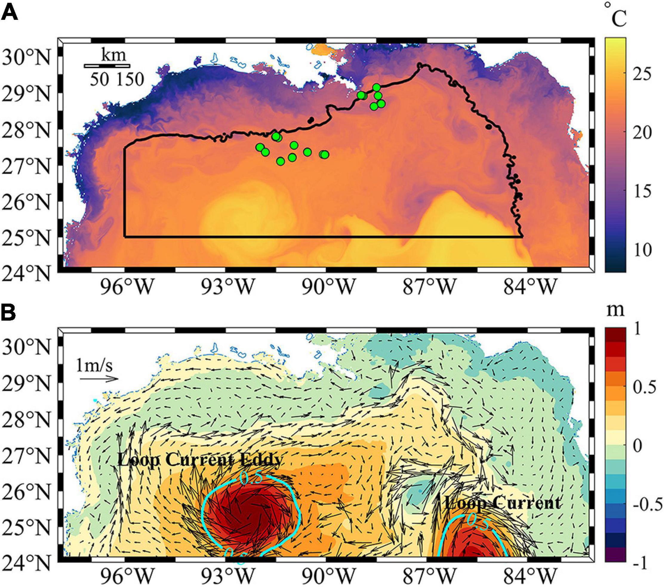
Figure 1. (A) Instantaneous surface temperature of the Gulf of Mexico at 00:30 GMT February 4, 2015. The black curve highlights the region where passive Lagrangian particles are released. Green dots indicate sampling locations for a 2015 summer cruise used to evaluate the model’s performance (see Supplementary Figure 1). (B) Corresponding instantaneous modeled sea surface height (SSH) field with superimposed surface flow velocities. Contours indicate 0.5 m SSH isobaths. In all snapshots throughout the paper, the time is 00:30 GMT.

Here, we use a regional ocean model to simulate the 3-dimensional transport of Lagrangian particles in the northern portion of the GoM, adopting a configuration similar to that in Luo et al. (2016). We consider a submesoscale permitting simulation at 1 km horizontal resolution and a mesoscale resolving 5 km horizontal resolution run, and release more than 20,000 neutrally buoyant particles multiple times over one year at different depths and in different seasons. Numerous previous works have focused on the impact of submesoscale circulations on transport and mixing on the horizontal component. Submesoscale circulations are responsible for increased horizontal mixing (Poje et al., 2014; Choi et al., 2017), while horizontal particle transport is mostly controlled by the mesoscale non-local dynamics (Taylor, 1921), and is nearly invariant whenever those are properly captured (e.g., Zhong and Bracco, 2013). Vertical transport, on the other hand, varies strongly with resolution (Thomas et al., 2008; Koszalka et al., 2009; Lévy et al., 2012; Zhong and Bracco, 2013). Although the submesoscale contribution to upwelling and downwelling motions have been previously discussed based on idealized numerical scenarios combined with theory (Mahadevan and Tandon, 2006; Mahadevan, 2016), a realistic quantification at regional scale is lacking. Our goal here is to explore the submesoscale contributions to upwelling and subduction within a modeling framework over a large portion of the Gulf of Mexico, whose dynamics are representative of tropical systems with an energetic mesoscale field. More specifically, we aim at identifying patterns and quantifying statistics of downwelling from the mixed-layer into the deeper ocean and of upwelling into the mixed layer from layers below.

Overview of the Gulf of Mexico Mesoscale and Submesoscale Circulations

In the GoM, the mesoscale circulation within the main thermocline is dominated by the Loop Current (LC) that enters the semi-enclosed basin through the Yucatan Channel and exits it through the Florida Straits (Figure 1B). The LC transports approximately 25 Sv (1 Sv = 1 × 10⁶ m³ s^–1) of warmer and saltier water from the equatorial Atlantic (Hamilton et al., 2005; Cardona and Bracco, 2014). At irregular intervals, but on average every 11 months (Vukovich, 1995; Sturges and Kenyon, 2008), mesoscale anticyclonic eddies up to 200–300 km in diameter detach from the LC. Their formation is only partially understood (e.g., Sturges and Lugo-Fernandez, 2005; Cardona and Bracco, 2014; Weisberg and Liu, 2017) and is influenced by the GoM bathymetry, the LC strength and the wind field. LC eddies extend to approximately 1,000 m in depth (Cooper et al., 1990; Forristall et al., 1992), propagate westward across the basin, and have a lifespan of many months, losing coherency through interactions with the continental shelf. The evolution of large mesoscale circulations controls to a great extent the exchange of biochemical tracers including nutrients and sinking organic particles in the GoM from the surface to depth and from the continental shelf to offshore waters (Schiller et al., 2011; Schiller and Kourafalou, 2014; Liu et al., 2018).

Seasonally varying river discharge strongly influences salinity and nutrient distributions, and the submesoscale circulations in the GoM (Luo et al., 2016; Barkan et al., 2017). In late spring and summer, the freshwater from the Mississippi-Atchafalaya River system reaches the LC and its eddies, transporting nutrients and sediments. Conversely, in winter the freshwater flow is generally weaker and remains more confined along the coastline due to the seasonal variation of wind stress. El Niño winters constitute an exception, due to the large precipitation increase usually occurring over the Mississippi watershed between December and April.

Submesoscale circulations extract available potential energy from the density gradients in the mixed layer (Molemaker et al., 2005; McWilliams, 2008). Previous studies have shown that in the open ocean the submesoscale seasonality follows therefore the variation of the mixed layer depth (MLD) (e.g., Mensa et al., 2013; Qiu et al., 2014; Callies et al., 2015). In the GoM, however, density gradients are contributed by not only the mesoscale circulations but also by the riverine outflow from the Mississippi-Atchafalaya River system (Luo et al., 2016). The riverine discharge both enhances submesoscale currents by providing lateral buoyancy gradients through the discharge of low salinity waters, and suppresses them by increasing stratification near the surface. Barkan et al. (2017) found that suppression is predominant in winter: the strength and number of baroclinic instabilities is slightly reduced compared to what would occur in the absence of freshwater forcing due to the increased near-surface stratification from riverine input. In late spring and early summer, when the freshwater discharge is usually greatest, the opposite is verified: submesoscale enhancement prevails despite the shallow mixed layer, with the generation of submesoscale fronts. Drifter experiments have confirmed the presence of these fronts (Poje et al., 2014) and numerical simulations have shown that if the river discharge is small or null, the formation of submesoscale circulations is indeed greater in winter and inhibited in summer (Luo et al., 2016).

Data and Method

We adopt the Coastal and Regional Ocean Community model (CROCO). CROCO is an oceanic modeling system built upon the Regional Ocean Modeling System (ROMS) in its Adaptive Grid Refinement in Fortran (AGRIF) version designed for simulating high-resolution offshore and nearshore dynamics (Shchepetkin and McWilliams, 2005; Debreu et al., 2012). This split-explicit, free-surface, and terrain-following vertical coordinate oceanic model is used to simulate the circulation in the GoM with horizontal resolution of 1 km (SP, for submesoscale permitting) and 5 km (MR, for mesoscale resolving) and 50 sigma layers in the vertical. Rotated mixing tensors for horizontal diffusion and the K-Profile Parameterization (KPP) vertical mixing scheme (Large et al., 1994) are applied as mixing parameterizations. Horizontal tracer advection is discretized with split and rotated 3rd-order upstream-biased advection scheme. The model bathymetry is derived from the 2-min Gridded Global Relief Data (ETOPO2) topography (Sandwell and Smith, 1997) interpolated to the model grid and modified to reduce horizontal pressure gradient errors using the Sikiric et al. (2009) method, with maximum slope factor (rx0) of 0.25 and maximum hydrostatic inconsistency number (rx1) of 15. The model domain covers the region between 98^o–82^o W and 24^o–31^o N (Figure 1) with open boundaries to the east and south sides that were nudged to the 6-hourly Hybrid Coordinate Ocean Model – Navy Coupled Ocean Data Assimilation (HYCOM-NCODA) Analysis system (GOMI0.04/expt_31.0)¹. The model is forced by six-hourly wind stresses and heat fluxes, as well as daily precipitation from the European Centre for Medium-Range Weather Forecast ERA-Interim reanalysis (Poli et al., 2010). No bulk formulas are used.

For the riverine forcing, the daily discharge by the five major rivers, Mississippi, Atchafalaya, Colorado, Brazos, and Apalachicola, is considered (Figure 2, blue line). These rivers consistently bring continental freshwater into the GoM with a flux rate of about 2.5 × 10⁴ m³ s^–1 from mid-March to mid-August of 2015, and a mean value of 1.2 × 10⁴ m³ s^–1 in other months. Discharge records from the United States Geological Survey (USGS)² are downloaded and converted to an equivalent surface freshwater flux that decays away from the river mouths with a length scale of 100 km at a constant rate as in Barkan et al. (2017). River momentum flux is therefore neglected. As shown in Barkan et al. (2017), their Figure 4, this treatment reproduces the observed surface salinity distribution offshore and in the narrow shelf regions surrounding the main Mississippi outflow reasonably well, but underestimates the freshwater content in the wide and shallow shelf to the west of the Atchafalaya River mouth.

FIGURE 2

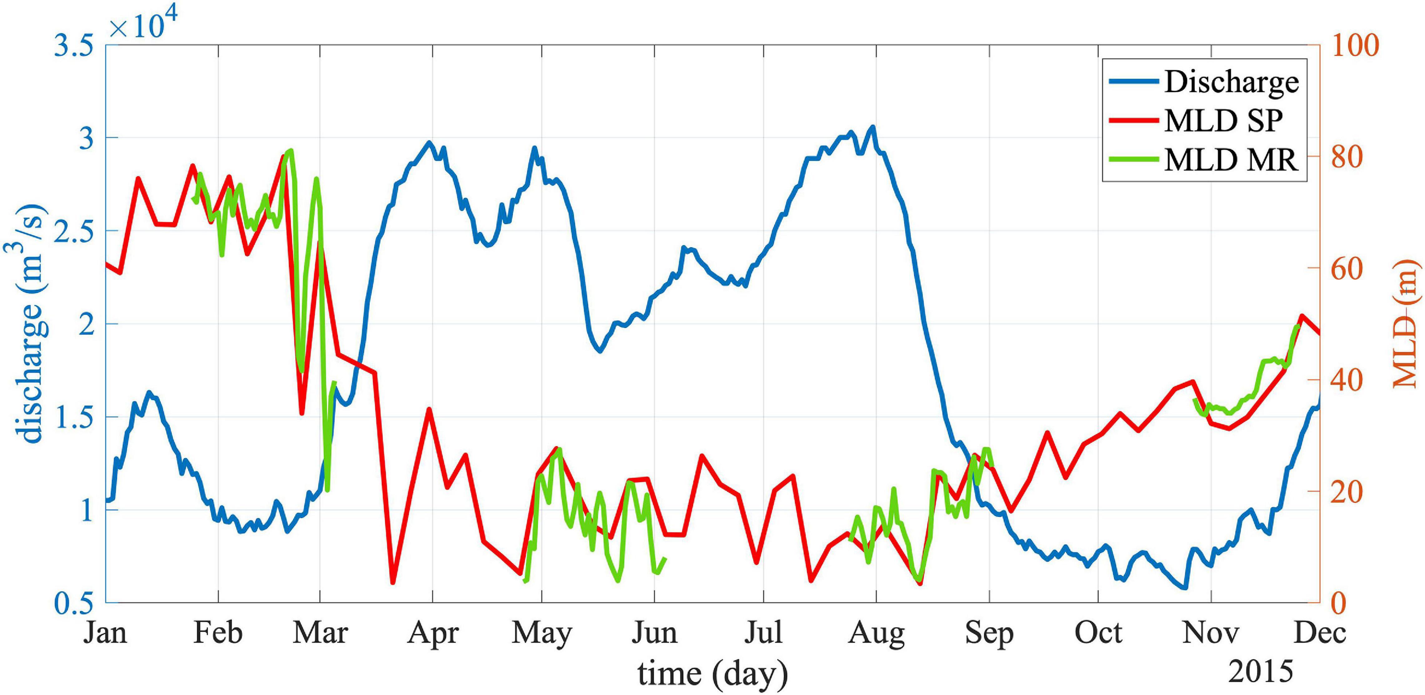
Figure 2. Mississippi River discharge (blue), 5-day averaged SP model MLD (red) in 2015 and daily averaged MR MLD (green) in our 4 periods during which Lagrangian tracers are released. Regions with ocean bottom depth shallower than 200 m are excluded from the MLD calculation.

A brief validation of the model representation of temperature and salinity in the upper 300 m of the water column is provided in the Supplementary Material (Supplementary Figure 1) against CTD profiles collected in 2015. The configuration further improves that in previous works and the validation of other fields or periods can be found in Luo et al. (2016); Cardona and Bracco (2014), Cardona et al. (2016b), and Sun et al. (2020).

We note that these solutions, while quite realistic in the representation of the mesoscale circulation and stratification of the basin, underestimate the internal wave field, due to the limited time and space resolution of the momentum forcing, the use of the hydrostatic approximation, and the lack of tidal forcing. The underestimation is comparable to that found by Beron-Vera and LaCasce (2016) in the HYCOM–NCODA solutions used here as boundary conditions.

The simulations cover the period September 31, 2014 to December 31, 2015 and our Lagrangian analysis focuses on February, May, August, and November in 2015, with more attention paid in the winter season when the submesoscale circulations are most intense. For the release periods we output 1-h averaged fields and used them to perform off-line Lagrangian integrations. In all cases, the particles are released north of 25^o N and east of 96^o W, limited by the 200 m isobaths to the north and east (Figure 1). They are tracked for at least 20 days using the advection module of the Larval Transport Lagrangian model version 2b (LTRANSv2b, Schlag and North, 2012) and their advection is determined by the Eulerian velocity field with no further diffusion added. Four releases are conducted in each period, with the same number of particles (21,874) deployed on different days. January 25, April 25, July 24, and November 1, 2015 represent Day 1 of the first winter, spring, summer and fall releases, respectively, and three more sets of particles follow after 10, 15, and 20 days in each case.

Three release plans have been considered in this work, indicated as surface, subsurface type 1 or type 1 in short, and subsurface type 2 or type 2, in the following. First of all, 21,874 passive Lagrangian particles are uniformly released near the ocean surface at 5 m depth (surface release). The same number of particles is then released below the base of the average (over the release domain) mixed layer. In winter the domain average MLD is about 80 m, while in summer is only about 15 m due the strong surface stratification, in agreement with sampling measurements (Weatherly, 2004). The chosen release depths are: 100 m in February, 50 m in May and November and 20 m in August (type 1 release). Since the mixed layer depth is spatially heterogeneous in the GoM, a portion of type 1 particles are released above the local mixed layer in all seasons. In winter this is verified for most particles released inside the LC eddies where the MLD reaches on average 120 m and can be as large as 150 m in the core of the eddies. This portion represents 18% and 16% of the total number of particles deployed in the SP and MR cases, respectively, independently of seasons. To better investigate cross-isopycnal mixing we deploy, only in winter, 21,874 particles 20 m below the base of the local mixed layer calculated at each particle position (type 2 release). In light of the strong riverine fluxes we opted for a MLD definition based on a temperature-only criterion as the depth at which the temperature difference from the surface is equal to 0.2^oC, following Luo et al. (2016). We verified that using instead a density-based definition with a density threshold from the surface to the base of the MLD of 0.03 kg m^–3 does not affect significantly our results (Supplementary Figure 2).

Results

Submesoscale Circulations in the GoM

As mentioned, the submesoscale circulations in the GoM vary seasonally and are modulated by the depth of the mixed layer, by the freshwater discharge, and by the density gradients associated with the Loop Current (LC) and the detached LC Eddies.

The abundance of submesoscale features in the GoM and their linkage, especially in summer, with the salinity distribution in the SP run is highlighted by snapshots of surface salinity (Figure 3) and relative vertical vorticity normalized by the planetary vorticity ζ/f (Figure 4) in all seasons. The vertical component of the vorticity vector is ζ = ∂v/∂x-∂u/∂y, being u and v the zonal and meridional components of the velocity. The vorticity field is filled with submesoscale eddies, filaments and fronts. Submesoscale eddies can be found also inside the LC eddy in winter, frontal structures surround the eddies in all seasons, and a “submesoscale soup” is evident throughout the year between the large mesoscale structures (for example between 90^oW and 84^oW in the winter snapshot). In the MR case, the mesoscale patterns are similar to that of the SP runs except for the slightly different Ring location (Supplementary Figures 3a–d). This small difference emerges due to the internal variability of the ocean system given that the simulations do not include data assimilation but only share the southern and eastern boundaries and the surface forcing.

FIGURE 3

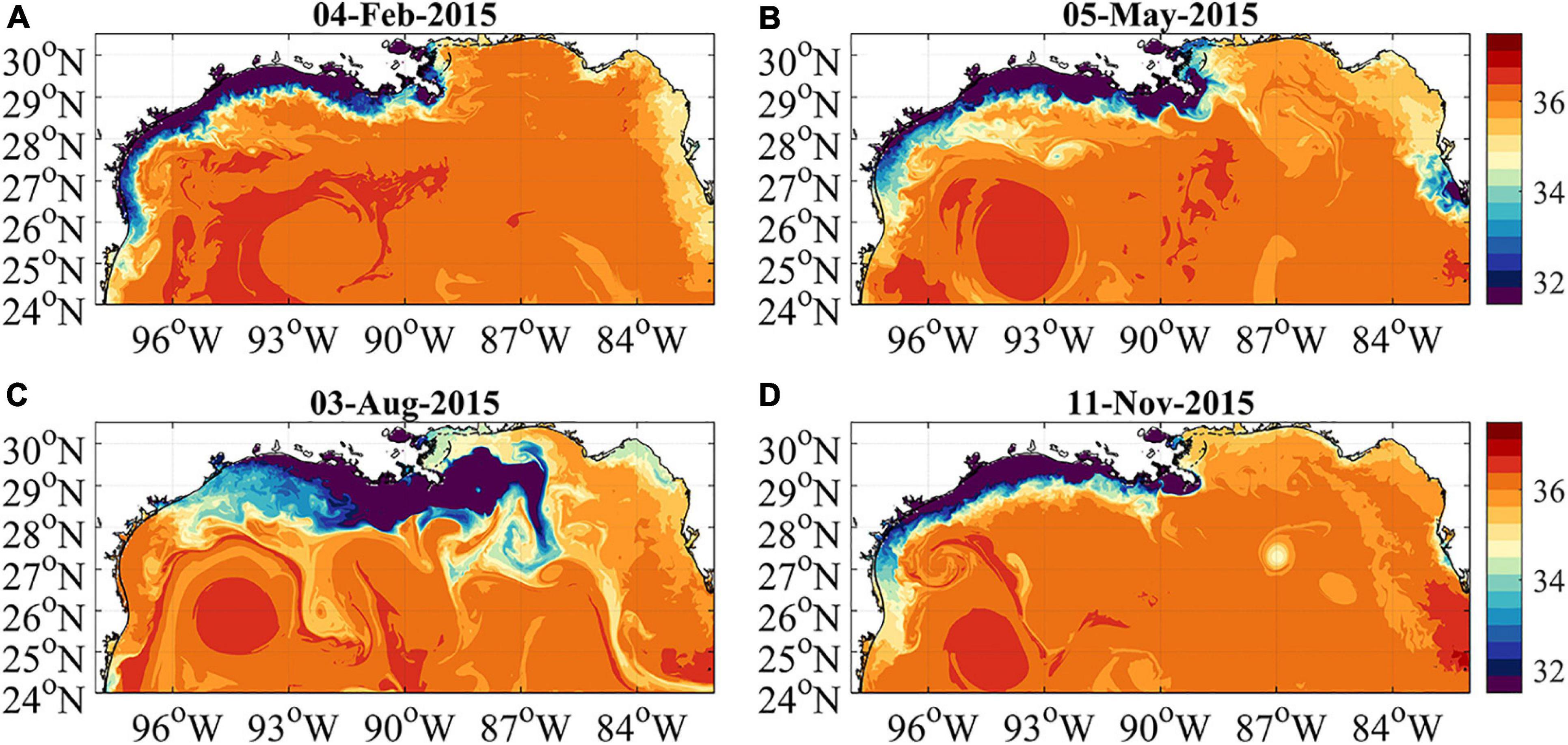
Figure 3. Instantaneous surface salinity fields in February (A), May (B), August (C), and November (D) 2015 in the SP simulation.

FIGURE 4

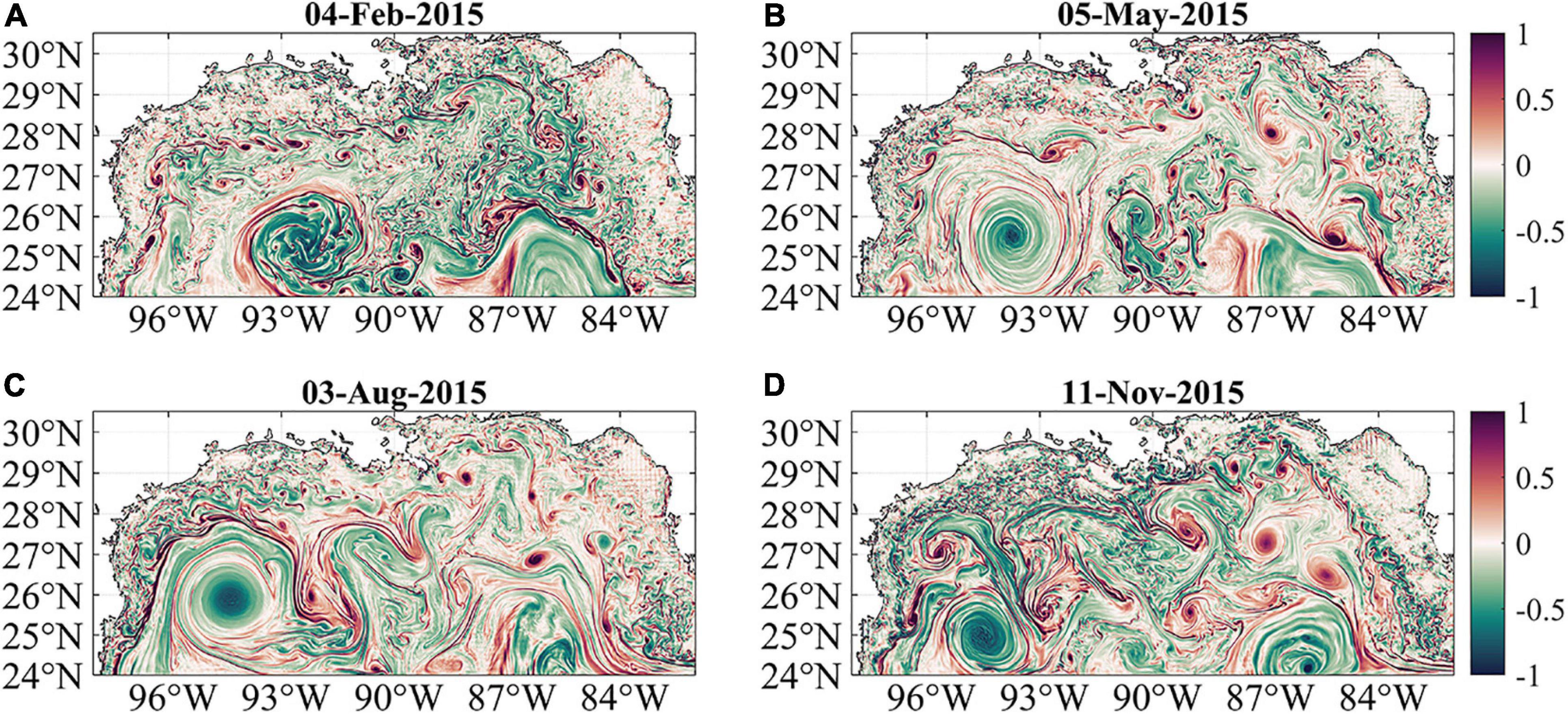
Figure 4. Relative vorticity fields normalized by the Coriolis frequency ζ/f in February (A), May (B), August (C), and November (D), 2015 in the SP simulation.

The prevalence of submesoscale circulations in the SP run, and especially of submesoscale cyclonic features (e.g., McWilliams, 2016) is quantified by the large positive tail in the relative vorticity probability density function (PDF, Supplementary Figure 3e). The PDF is constructed using hourly saved vorticity snapshots from the first week of February 2015. The asymmetry in the tails decreases sharply with depth and nearly disappears below the mixed layer (see distribution at the depth of subsurface type 2 release in Supplementary Figure 3e). In the MR run the asymmetry is far reduced compared to the SP case.

Seasonal Distribution and Transport of Lagrangian Particles

In the present investigation, the impact of mesoscale and submesoscale motions on tracer dispersion in the GoM is investigated by deploying Lagrangian particles at different depths and in different months over most of the model domain (i.e., not targeting specific structures as done, for example, in Zhong et al. (2017). Figure 5 shows the distribution of particles released at 5 m depth after 10 days in the four seasons in the SP run. It demonstrates also the strength of vertical transport in winter, followed by fall, spring and then summer. The mixed layer is deepest in winter and most particles released near the surface reach quickly depths of 50 m. Conversely, in other seasons, the average depth covered by the particles in 10 days is only ∼10 m. In the MR case a similar seasonal dependence is demonstrated, but the mean vertical displacements have a smaller magnitude, despite the comparable mixed layer depths (Supplementary Figures 4a,b).

FIGURE 5

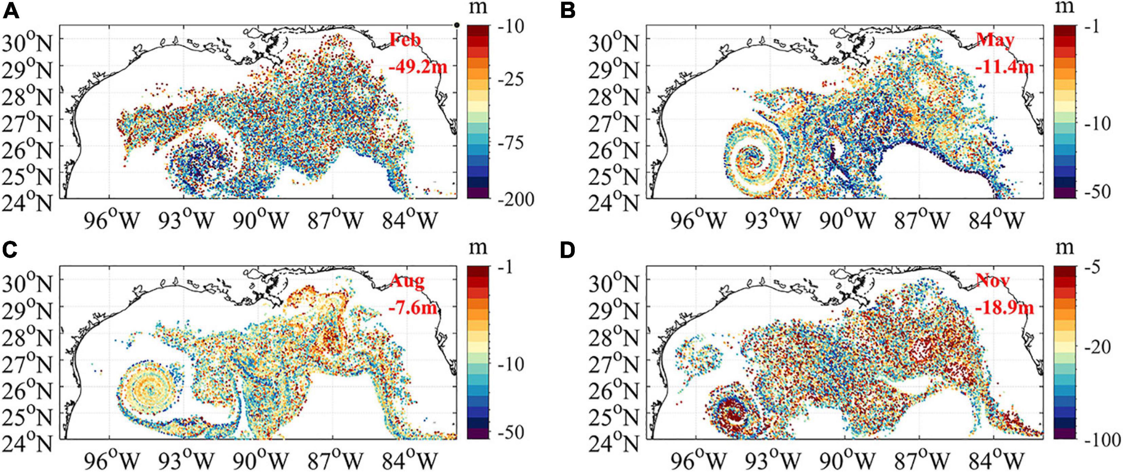
Figure 5. Distribution of Lagrangian particles released at 5 m depth (surface) after 10 days in the SP simulation in February (A), May (B), August (C), and November (D). Color shading in logarithmic scale indicates the depth of each particle and varies across seasons. The mean depth of the particles on day 10 is also indicated. The particles plotted are from the first release in each season.

For particles released below the mixed layer (both type 1 and type 2 releases), the lateral pattern and seasonal variations are similar to those of the near-surface release (Figure 6, shown only for February and August). Upward movements are observed in the winter season especially inside the Ring and in the northeastern region where small-scale filaments and submesoscale vorticity dominate. The initial depth distribution of type 2 particles is also shown (Figure 6D). For the lower resolution run (Supplementary Figures 4c,d), the vertical spreading of tracers is narrower and upwelling is found mostly around the LC eddy. In summer upward movements are restricted to a narrow depth range at both resolutions (Figure 6B), and are only detectable in the alignments and spiraling structures around the LC and the Ring.

FIGURE 6

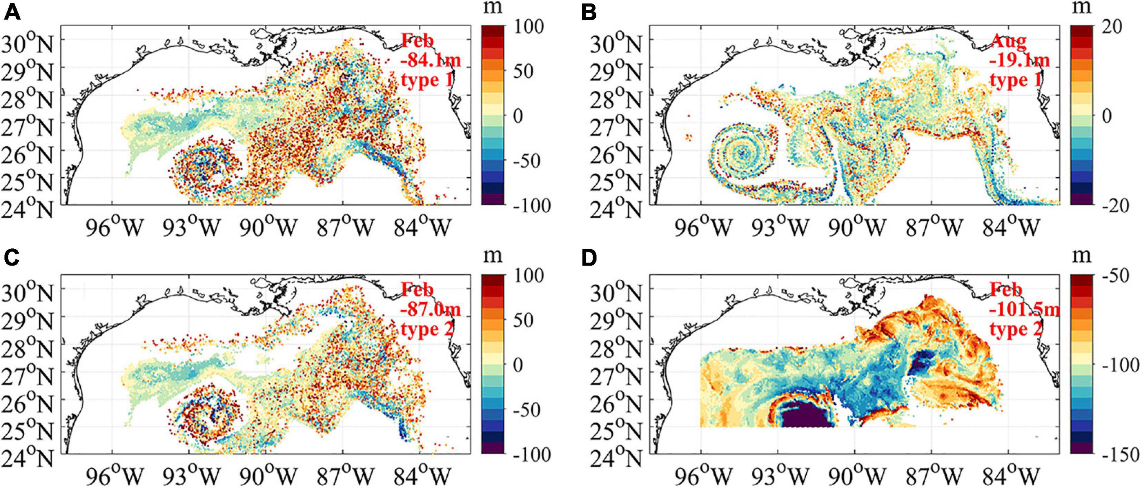
Figure 6. Distributions of depth changes for “deep” Lagrangian particles after 10 days in the SP simulation in February [(A): release type 1, initial depth 100 m] and August [(B) release type 1, initial depth 20 m]. Positive values indicate upwelling. (C): distribution depth changes for type 2 particles, always after 10 days and (D): the initial depth of the type 2 particles in panel (C). Particles that have traveled horizontally more than 300 km have been removed. The mean depth of the particles on day 10 is also indicated. The particles plotted are from the first release in winter and summer.

A quantification of the vertical spreading is provided by Supplementary Figures 5, 6, showing the time evolution of the averaged depth of the particles (a-b), the percentage of particles moving upward or downward (defined as vertical displacement larger than 4 m up or down) (c-d), and the absolute vertical dispersion (e-f) for the releases at 5 m and below the MLD in winter and summer (Supplementary Figure 5), and in spring and fall (Supplementary Figure 6), respectively. The absolute vertical dispersion is defined as A²(t) = < | z_i(t) – z_i(t₀)| ² >, where z_i(t) and z_i(t₀) describe the vertical position of particle i at time t and at release time t₀, and < > represents the average over all particles. The dispersion curves show that the higher resolution is associated with overall larger dispersions, in agreement with previous studies (e.g., Zhong and Bracco, 2013; Zhong et al., 2017). This behavior is independent of season qualitatively, while follows, as to be expected, the seasonal cycle of the submesoscale structures in strength.

Upwelling and Downwelling Processes

Next, we focus on the winter season, when the submesoscale circulations are the most intense and vertical displacements the largest, to further investigate the patterns of upwelling and downwelling motions. The conclusions we draw extend to other seasons, but the range of vertical displacements is more limited, especially in summer. Additionally, results on vertical mixing patterns agree between winter 2015 and winter 2016, although results from the later winter are not shown for clarity, being the mesoscale field significantly different.

Figure 7 shows the 2-dimensional kernel density estimation (KDE) of the horizontal distribution of the particles after 10 days since their release calculated using all available deployments (4 in each panel). The KDE is a non-parametric technique for density estimation and in this case indicates how particles are distributed laterally, independently of their depth, in each grid point. Here it has been normalized so that a value of 1 is indicative of a homogenous distribution (the initial distribution satisfies the condition). Independently of resolution, a higher density of particles than at release time is found within the Ring. The outer boundaries of the LC and of the Ring emerge as lower than average density areas due to the strong divergence found at the boundary of the mesoscale structures (see e.g., Luo et al., 2016), while the regions occupied by an energetic submesoscale soup north and west of the LC (see Figure 4A) have densities slightly higher than 1 in the SP case. In the MR run the Ring is more impermeable to outward fluxes and concentrate particles over a larger area, while the region north of the LC that shows some indication of submesoscale instabilities (Supplementary Figure 3a) is also slightly denser than at release time. Overall, the lateral distribution of the particles is similar across resolutions, as to be expected being the absolute lateral dispersion controlled by the non-local mesoscale processes (Taylor, 1921).

FIGURE 7

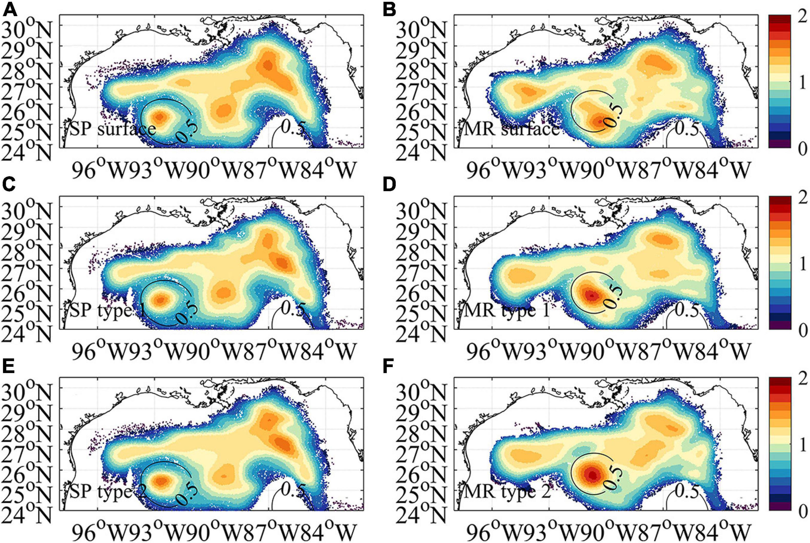
Figure 7. Horizontal distributions of the 2-dimensional KDE of all particles (from all ensembles) after 10 days since their release in SP (A,C,E) and MR (B,D,F) simulations. The type of release is indicated in each subplot. The KDE is normalized to indicate a homogenous distribution at KDE = 1.

In the vertical, on the other hand, stronger submesoscale-induced upwelling and downwelling are observed in the SP case and are associated with steeper slopes in the first few days of the absolute dispersion curves in Supplementary Figure 5. The MR run, on the contrary, maintains a much greater concentration of particles around their release depth, either near the surface or below the average or local mixed layer depth. The time evolution of the percentage of particles undergoing a given depth variation in one of the 2015 winter deployments (Figure 8) highlights that the SP/MR differences are quite large for the first couple of weeks and reduce thereafter.

FIGURE 8

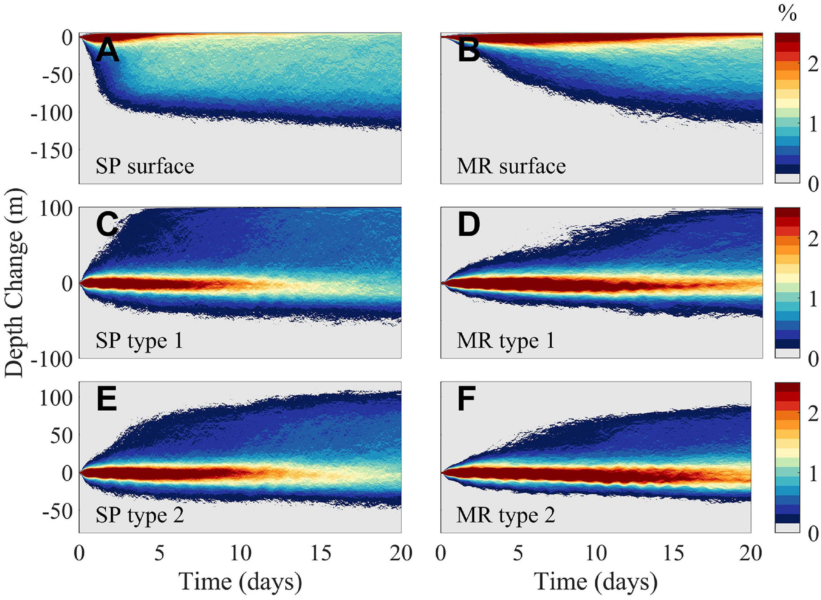
Figure 8. Time evolution of the depth variation of particles in the first winter release (release date: January 25, 2015) expressed as percentage. The particles are released at a depth of 5 m (A,B), 100 m (C,D) and 20 m below the local mixed layer (E,F). SP run on left and MR run on the right.

To further identify the hot-spots where strong upwelling and downwelling occur, we use once more the KDE, applied to the absolute tracer displacement and to the mixed layer crossing (Figure 9). For the first case, i.e., absolute tracer displacement, we consider the surface and type 1 ensembles in which particles are released at a constant depth (5 or 100 m). We define as downwelling particles those released at 5 m that sink more than 88 m in 10 days, and as upwelling particles those released at 100 m depth that upwell to at least 34 m by day 10. Among the 21,874 particles initially released in each SP ensemble member, at least 3,000 satisfy the above definitions in all case. Other choices of the upwelling/downwelling criteria are possible and thresholds have been chosen only to ensure a comparable number of particles across runs. We verified that other choices would return qualitatively similar results (Supplementary Figure 7). For the mixed layer crossing, we compare the surface and type 2 releases and consider the particles’ relative position with respect to the mixed layer again 10 days after their release. Particles released at 5 m that move downward across the mixed layer are labeled as downwelling, and those that upwell above 0.48 × MLD as upwelling. Again, at least 3,000 particles cross the mixed layer in either direction in each ensemble.

FIGURE 9

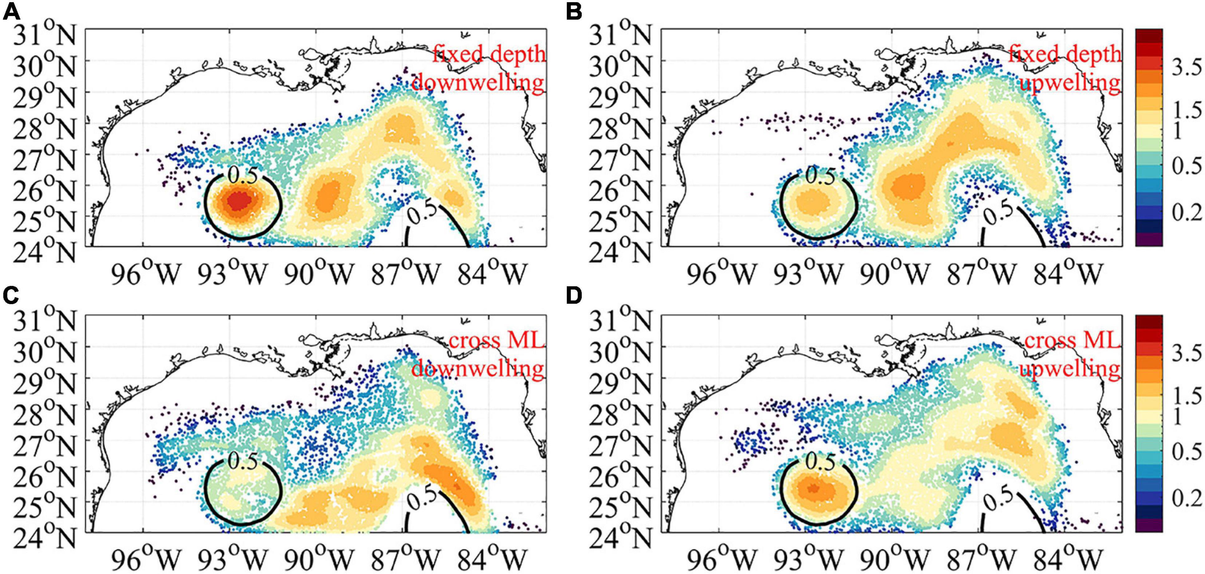
Figure 9. KDE of particles selected based on their vertical absolute displacement after 10 days (A,B) and cross-mixed layer behavior (C,D) calculated considering all four winter SP releases (see text for details). The particles are initially released at 5 m [panels (A,C) labeled as “downwelling”] and at deeper depths [(B) release type 1; (D) release type 2, labeled as “upwelling”]. Black contours indicate the 0.5 m sea surface height isobaths and outline the location of the LC and the Ring.

In the absolute vertical displacement case (Figures 9A,B), strong downwelling and upwelling activities are found within the Ring at about 92.5^oW and 25.5^oN. The downward branch has higher density values (yellow colors) in the eddy, indicating that although efficient upward and downward fluxes exist in the large anticyclone, the downwelling component dominates as a result of the depression of isopycnal surfaces. This behavior is in agreement with applications of the omega equation based on the quasigeostrophic theory (Hoskins et al., 1978). Large amplitude downward and upward movements of particles, larger than predicted by the omega equation (Koszalka et al., 2009) are found within the eddy, in agreement with the analysis in Zhong et al. (2017). As in the South China Sea anticyclone investigated in Zhong et al. (2017), ageostrophic vertical velocities in submesoscale fronts where symmetric instabilities can easily develop are responsible for enhancing the vertical transport in both the circulation cell that delineates the outer edge of the Loop Eddy and in its core. Large movements are also present in the areas with the strongest submesoscale vertical velocities accompanied by a deep mixed layer, i.e., in the “submesoscale soup” and at the periphery of the LC eddy and in the region between the Ring and the LC. Upwelling and downwelling patterns are similar among them and across ensemble members. These similarities indicate that upward and downward fluxes are always active under the influence of strong submesoscale circulations, as to be expected.

The mixed layer crossing (Figures 9C,D), on the other hand, follows different patterns. A high density of downward particles is found at the periphery of the LC where the MLD is shallow (∼40 m) and submesoscale fronts are intense, low density characterizes the core of the LC eddy, where the MLD reaches values as large as 150 m, and isolated particles can be seen in the submesoscale-soup areas. Greater uniformity (more values of the KDE between 0.75 and 1.25) is found for particles entering the mixed layer from below in the submesoscale dominated areas with the exception of the Ring. Overall, 43.1% of the KDE values in the “soup” region (simply defined as the release area excluding the Loop Eddy within the 0.5 m SSH anomaly) indicate uniformity for the upward crossing versus less than half (19.8%) in the downward case (Figure 9C). This is further quantified by the lower standard deviation of the KDE in the “soup” region in the upwelling case compared to the downwelling one – 0.61 versus 0.40, respectively. In the SP run the Ring is a preferential location for upwelling into the mixed layer, and the upwelling and downwelling patterns are far less similar than in the fixed-depth case.

The corresponding analysis has been performed on the MR case, where strong upwelling and downwelling are limited to ∼500–800 particles per ensemble member (Figure 10). In the absolute displacement case (Figures 10A,B), the largest downwelling is concentrated in the LC eddy in the center of the domain, around the LC and to the north of it, where the vorticity is anticyclonic, while upwelling occurs inside the (moving) LC eddy and appears stronger than the downwelling branch. Mixed layer crossing in its downwelling component is achieved only at the periphery of the LC, where the MLD is shallowest, while upwelling is more uniformly distributed to the north of the LC, where frontal structures are present. Noticeably, no upwelling occurs across the mixed layer boundary within the Ring in MR, while being a common occurrence in SP. In addition to wind-eddy interaction and frontogenesis, the cause of intense submesoscale upwelling detected in anticyclonic eddies has been linked to symmetric instability that extracts kinetic energy from the geostrophic flow (Thomas et al., 2013; Brannigan, 2016; Zhong et al., 2017).

FIGURE 10

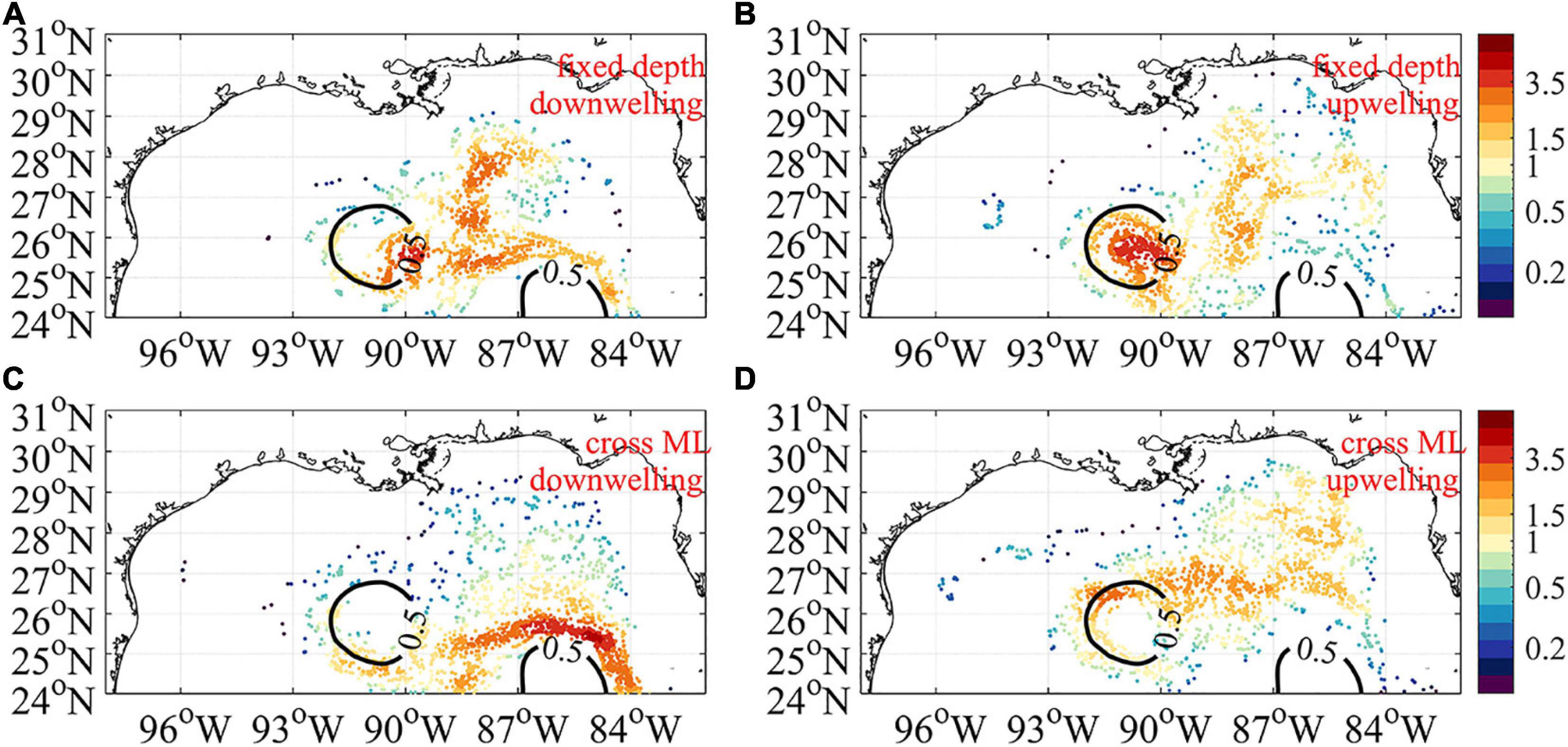
Figure 10. KDE of particles selected based on their vertical absolute displacement after 10 days (A,B) and cross-mixed layer behavior (C,D) calculated considering all four winter MR releases. The particles are initially released at 5 m [panels (A,C) labeled as “downwelling”] and at deeper depths [(B) release type 1; (D) release type 2, labeled as “upwelling”]. Black contours indicate the 0.5 m sea surface height isobaths and outline the location of the LC and the Ring.

Figures 8, 9 indicate that there is an asymmetry with a preference toward upwelling motions into the mixed layer for type 1 and type 2 particles in both runs, particularly at the longitude of greatest submesoscale activity (east of 90^oW), compensating for the prevalent downwelling out of the surface layer. In the SP run the upwelling into the mixed layer occurs more frequently and is much stronger than in the MR case, especially underneath the “submesoscale soup.” This is visualized in Supplementary Figure 8 where the particles from one of the ensemble members are plotted along a transect at 87^oW in both runs.

The joint probability distribution of the vertical velocity and relative vorticity calculated at the particle position outside the Loop Eddy one day after their release is shown in Figure 11 for the surface and type 2 particles in the two runs. The strongest downwelling (large negative w) is favored for positive vorticity values in the SP case (Figure 11A), in agreement with previous studies (Mahadevan and Tandon, 2006). In the MR run (panel b), on the other hand, w values are always small and nearly symmetrically distributed in the vorticity space. Below the mixed layer (Figures 11C,D), the joint distribution is nearly symmetric and the upwelling into the mixed layer is not associated to structures with a preferential vorticity sign in both cases, with larger vertical velocities attained in the SP case (panel c).

FIGURE 11

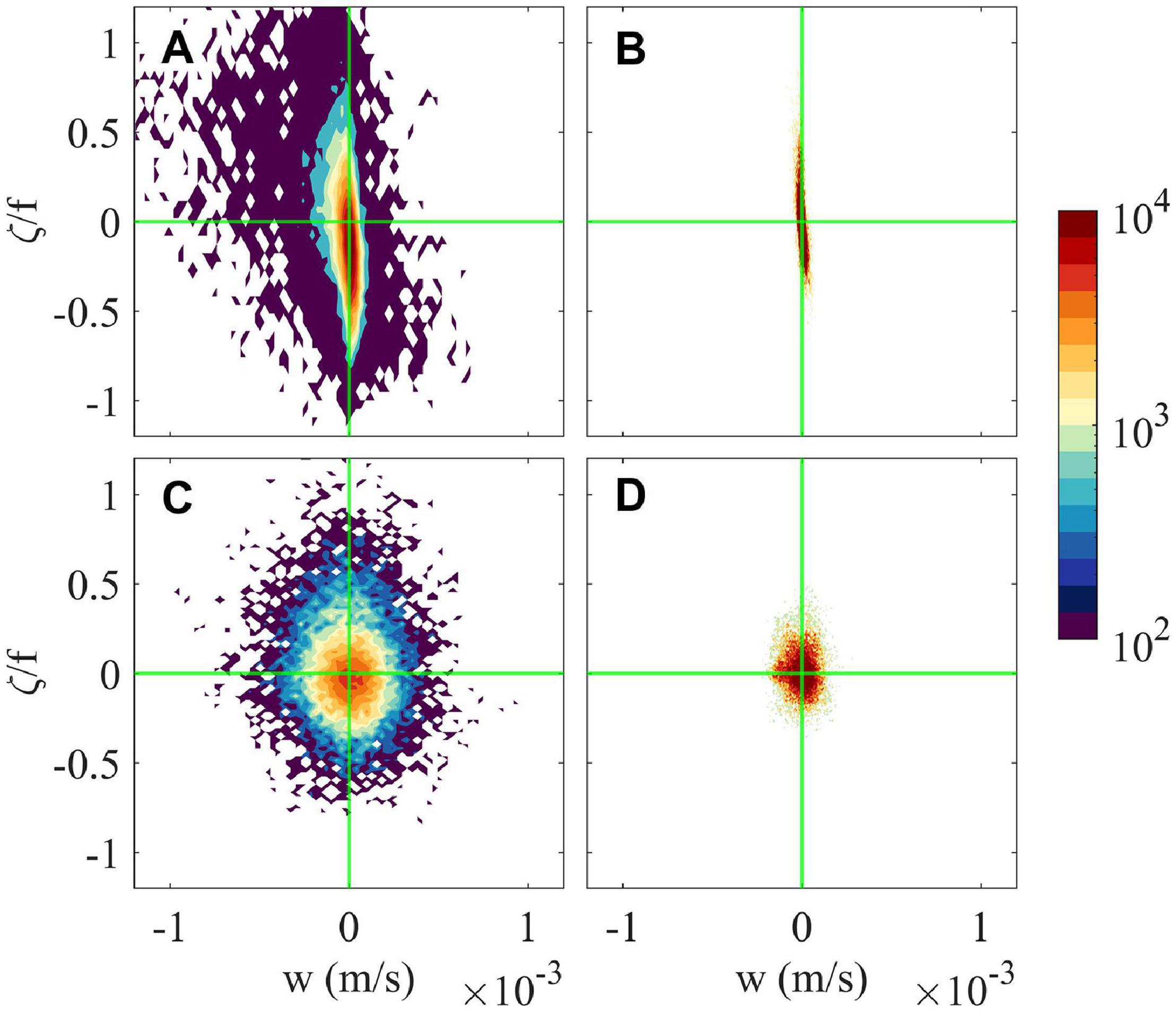
Figure 11. Joint probability density function of vertical velocity and relative vorticity based on particles position 24 h after deployment in the SP (A,C) and MR (B,D) simulations, for surface (A,B) and type 2 (C,D) releases. Green lines indicate values of zero. The distributions are calculated using the first SP and MR releases in winter.

Finally, we have used the tracers to quantify the impact of resolution on the vertical spreading of the Lagrangian tracers in terms of diffusivities. We computed the vertical diffusivity coefficients as time derivative of the (vertical) relative dispersion, R², defined as R²(t) = < | z_i(t) −z_j(t)| ² >, where z_i and z_j are the position of two initially nearby particles at time t, and < > indicates the average over all particle pairs. Pairs were defined by particles in nearby grid cells, as in Bracco et al. (2016). Figure 12 shows the diffusivity for surface and type 2 releases at the two resolutions from the fourth day after the particle release, once the diffusivity has stabilized. The SP run is characterized by nearly an order of magnitude greater spreading in both cases, with k_z approximately 1.4 × 10^–3 m² s^–1 and 9.6 × 10^–4 m² s^–1 for surface and type 2 particles, respectively, in agreement with the indirect estimates from in situ sampling of nutrient fluxes in the upper 100 m of the water column off Concepción, Chile presented in Corredor-Acosta et al. (2020). The system is neither unbounded nor homogeneous, and the model uses the KPP parameterization, therefore interpreting the relative dispersion slope in terms of turbulent theories is not possible. However, the fact that the SP results are in-line with the (limited) observations, while the MR run underestimate k_z by an order of magnitude points to a quantification of the role of submesoscale-induced vertical mixing in the upper ocean.

FIGURE 12

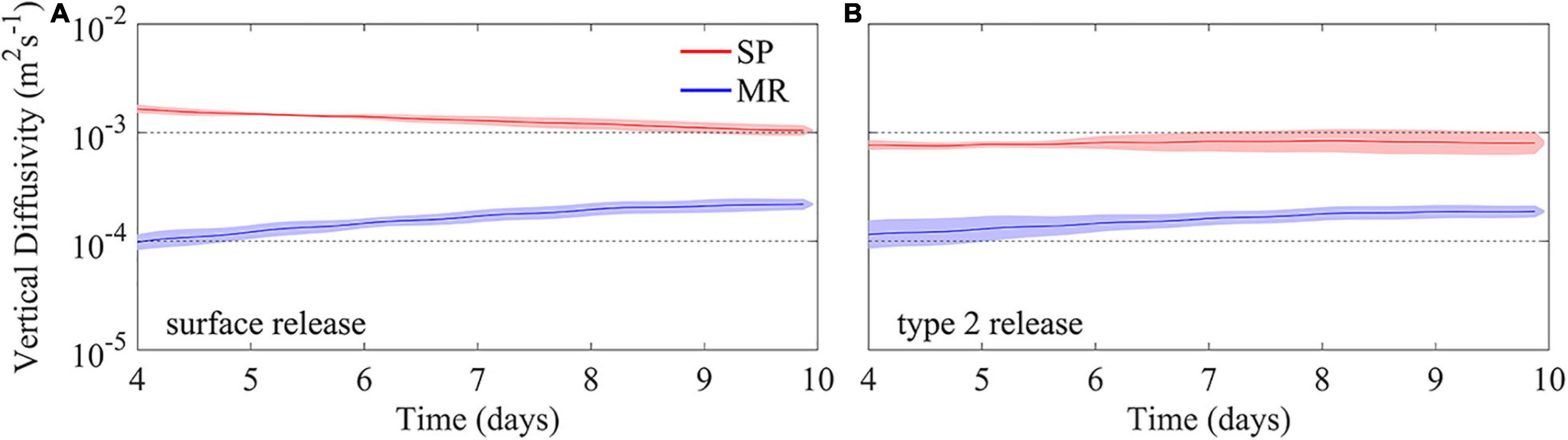
Figure 12. Vertical diffusivity coefficients for surface (A) and type 2 (B) releases at the two resolutions in the 4–10 days period after their release in February 2015. The value is averaged over all ensembles, color shading corresponds to standard deviation.

At last, Figure 13 displays the lateral variability of k_z in the model domain through diffusivity maps for surface and type 2 releases at the two resolutions. Particle couples are grouped into different bins based on their release location, and the mean diffusivity for each bin is calculated using the particles’ 10-day trajectories. Bins with less than 15 couples are omitted and the calculation is repeated on each ensemble members and then averaged. In the SP run the mesoscale Ring emerges clearly as hotspot for vertical mixing, in agreement with the eddy-focused analysis by Zhong et al. (2017), while lower than average diapycnal mixing is found within the Ring in the MR case, confirming the KDE results. Additionally, the eastern and central portions of the Gulf, more strongly impacted by the vigorous Loop Current and by the riverine fluxes, and therefore by more intense mesoscale and submesoscale variability, have greater overall diffusivities than the western portion of the basin. This east-west gradient is found in both solutions.

FIGURE 13

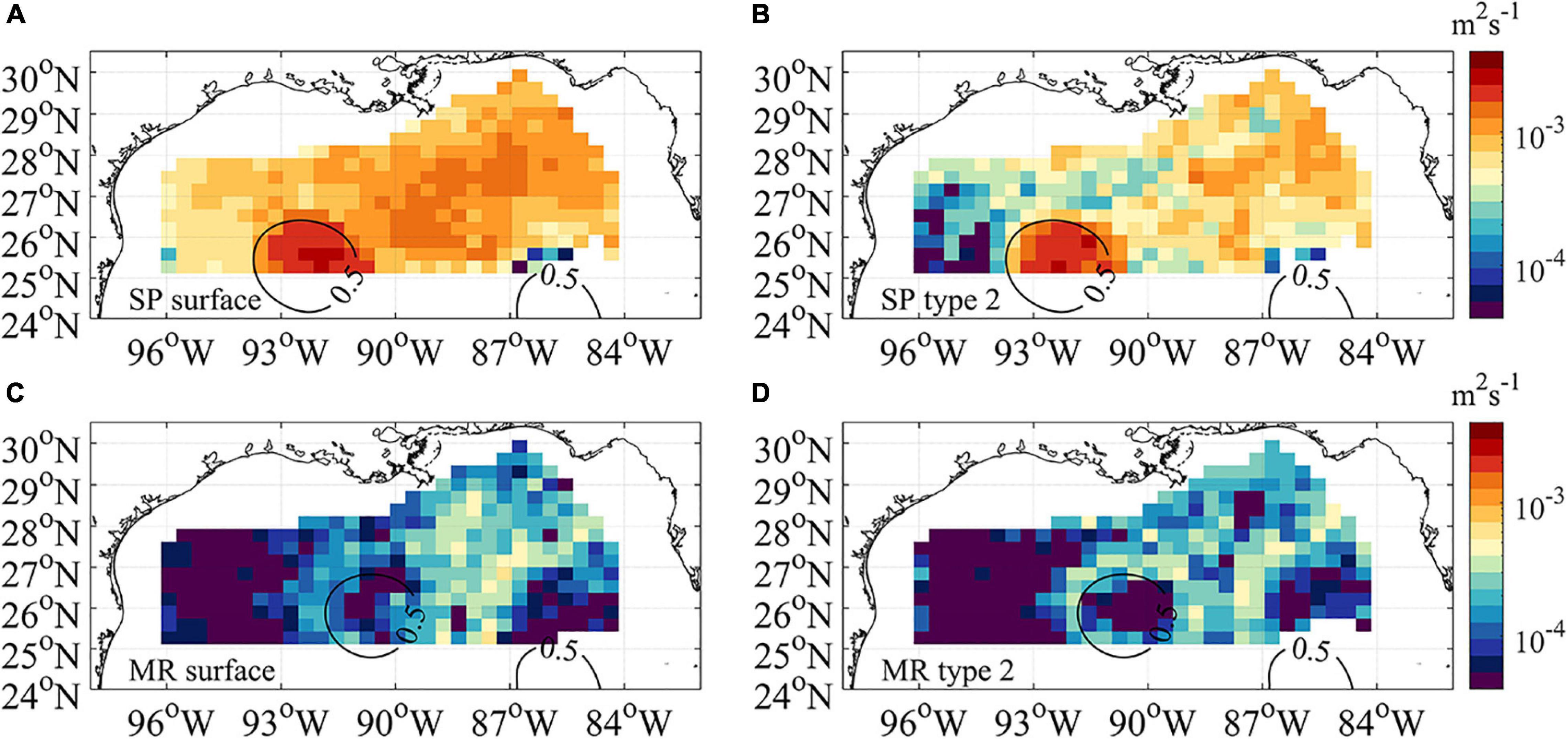
Figure 13. Maps of binned vertical diffusivity for surface (A,C) and type 2 (B,D) releases at the two model resolutions [SP (A,B); MR (C,D)] in February. Particles are first binned based on their initial location. The 10 days particle trajectories of each bin are then used for diffusivity calculation. Results from day 4 to 10 are averaged and denote the diffusivity for each bin. Contours are 0.5 m SSH isobaths.

Discussion

We performed model integrations in the northern GoM at submesoscale permitting (SP, 1 km) and mesoscale resolving (MR, 5 km) resolutions, and analyzed Lagrangian trajectories to quantify transport and mixing across the mixed layer. Over 20,000 passive particles were released uniformly at a depth of 5 m (i.e., surface) and below the domain-averaged (type 1) or local mixed layer (type 2) multiple times and in different months in 2015 to simulate the seasonal exchange of particles between the surface and the deep ocean. With respect to previous works (e.g., Zhong and Bracco, 2013; Zhong et al., 2017) here we investigated the behavior of particles distributed uniformly over the whole model domain, without focusing on specific structures, and we explored both downwelling and upwelling motions. The overarching question we aimed to address is: where do upwelling into, and downwelling from, the mixed layer occur whenever in presence submesoscale dynamics in the northern GoM? Our results confirm that higher model resolution leads to stronger vertical velocities that are associated with submesoscale structures (Capet et al., 2008; Lévy et al., 2012; Zhong and Bracco, 2013). This submesoscale-induced velocity results in an order of magnitude more effective exchange of particles in the vertical direction, both upward and downward, that lasts from hours to few (order 10) days, and one order of magnitude greater vertical diffusivities. The submesoscale contribution to vertical advection impacts directly the euphotic layer and influences the upper ocean ecosystem by redistributing nutrients, larvae, and other organic matters and is not uniform in its upwelling/downwelling contributions or even laterally within a basin as small as the Gulf of Mexico.

Outside the LC eddy (i.e., in the region that would be identified as “submesoscale soup” following McWilliams, 2016) upwelling into the mixed layer is more uniformly distributed than downwelling out of it (Figures 9C,D). The Ring, on the other hand, is a vehicle for particle upwelling in the submesoscale permitting case, as already found in the South China Sea (Zhong et al., 2017).

The upwelling/downwelling patterns are consistent across seasons, but the relative role of submesoscale motions compared to mesoscale ones in setting vertical transport is far greater in winter than during the rest of the year. It is worth mentioning that in the GoM the nutricline is found at the base of the mixed layer only in winter and primary productivity is high from the surface to the depth of the chlorophyll maximum (about 100 m) just in this season (Damien et al., 2018). Our results call for a major contribution of submesoscale vertical mixing in upwelling nutrients into the mixed layer to support productivity across the whole mixed layer in winter in a nearly homogenous way outside large mesoscale eddies. In spring, summer and fall, the chlorophyll maximum is significantly deeper than the mixed layer, and submesoscale-induced upwelling has likely a limited influence on productivity. The downwelling of particles below the mixed layer (i.e., the cross-mixed layer transport from the surface downward), on the other hand, is affected by the submesoscale circulations year around.

As note of caution, a resolution of 1 km is insufficient to capture the rate of convergence at the ocean surface in the Gulf of Mexico (Barkan et al., 2019; Sun et al., 2020) and higher than 1 km horizontal resolution may be needed. Additionally, the upper few centimeters of the water column are characterized by very strong vertical velocity magnitudes (Laxague et al., 2018), and therefore large convergence/divergence fluxes, that are not captured by current hydrostatic ocean models. On the other hand, below the upper 10–20 m from the ocean surface, simulations at 1 km horizontal resolution reproduce quite accurately the few submesoscale permitting observations of vertical velocities and shear available (see Zhong et al., 2017 for sampling in/around an anticyclone of size and strength comparable to a Loop Current eddies, and Zhong and Bracco (2013) for a model-data comparison based on ADCP measurements in the GoM). Increasing horizontal resolution in hydrostatic runs implies overestimating vertical velocities and their standard deviations. We opted for a conservative submesoscale permitting quantification in this work, and we plan to further decrease the grid size adopting a non-hydrostatic model in the near future.

Data Availability Statement

The datasets presented in this study can be found in online repositories. The names of the repository/repositories and accession number(s) can be found below: Data have been submitted to the Gulf of Mexico Research Initiative Information & Data Cooperative (GRIIDC) at https://data.gulfresearchinitiative.org/data/R4.x268.000:0129 in May 2020. Pre-processed datasets and codes are available at GitHub: https://github.com/gliu87/Pre-processed-Data-and-Code-for-MLD-Paper. Requests to access the model output should be directed to the authors.

Author Contributions

GL performed the simulations and conducted analyses. AS performed the model validation and contributed to the analysis. GL, AB, and AS drafted the manuscript and contributed to discussions, interpretations, and writing. All authors designed the study, read, and approved the submitted version.

Funding

The research was made possible in part by a grant from The Gulf of Mexico Research Initiative through the ECOGIG consortium. AB was supported by the National Science Foundation (OCE- 1658174).

Conflict of Interest

The authors declare that the research was conducted in the absence of any commercial or financial relationships that could be construed as a potential conflict of interest.

Supplementary Material

The Supplementary Material for this article can be found online at: https://www.frontiersin.org/articles/10.3389/fmars.2021.615066/full#supplementary-material

Footnotes

References

Barkan, R., McWilliams, J. C., Molemaker, J., Choi, J., Srinivasan, K., Shchepetkin, A. F., et al. (2017). Submesoscale dynamics in the northern Gulf of Mexico. Part II: temperature- salinity relations and cross shelf transport processes. J. Phys. Oceanogr. 47, 2347–2360.

Google Scholar

Barkan, R., Molemaker, M. J., Srinivasan, K., McWilliams, J. C., and D’Asaro, E. A. (2019). The role of horizontal divergence in submesoscale frontogenesis. J. Phys. Oceanogr. 49, 1593–1618.

Google Scholar

Beron-Vera, F. J., and LaCasce, J. H. (2016). Statistics of simulated and observed pair separations in the Gulf of Mexico. J. Phys. Oceanogr. 46, 2183–2199. doi: 10.1175/JPO-D-15-0127.1