Effects of Climate Change in Marine Ecosystems Based on the Spatiotemporal Age Structure of Top Predators: A Case Study of Bigeye Tuna in the Pacific Ocean

How top predators behave and are distributed depend on the conditions in their marine ecosystem through bottom−up forcing; this is because where and when these predators can feed and spawn are limited and change often. This study investigated how the catch rates of immature and mature cohorts of bigeye tuna (BET) varied across space and time; this was achieved by analyzing data on the Taiwanese longline fishery in the western and central Pacific Ocean (WCPO). We also conducted a case study on the time series patterns of BET cohorts to explore the processes that underlie the bottom-up control of the pelagic ecosystem that are influenced by decadal climate events. Wavelet analysis results revealed crucial synchronous shifts in the connection between the pelagic ecosystems at low trophic levels in relation to the immature BET cohort. Many variables exhibited decreasing trends after 2004–2005, and we followed the Pacific Decadal Oscillation (PDO) as a bottom-up control regulator. The results indicated that low recruitment into the mature cohort occurs 3 years after a decrease in the immature cohort’s food stocks, as indicated by a 3-year lag in our results. This finding demonstrated that, by exploring the connection between low-trophic-level species and top predators at various life stages, we can better understand how climate change affects the distribution and abundance of predator fish.

Introduction

Changes, anomalies, and oscillations in the climate affect numerous ecological processes in marine ecosystems, which in turn strongly affect the abundance and distribution of top predators, such as tuna, in the ocean (Langley et al., 2009; Syamsuddin et al., 2013; Goñi et al., 2015; Lan et al., 2019). Therefore, biological and oceanographic information concerning top predators can aid the management of fishery resources and fishing operations (Damalas and Megalofonou, 2012; Nieto et al., 2017). Previous studies have focused on the implications of thermal tolerance and on the environmental factors that limit the area over which top predators are distributed, doing so by using species distribution models and data from fisheries (Figure 1A). The availability of oceanographic and biological information can help parameterize the environmental characteristics that influence the range, habitats, and biology of the species of interest (Lehodey et al., 2010; Senina et al., 2020).

FIGURE 1

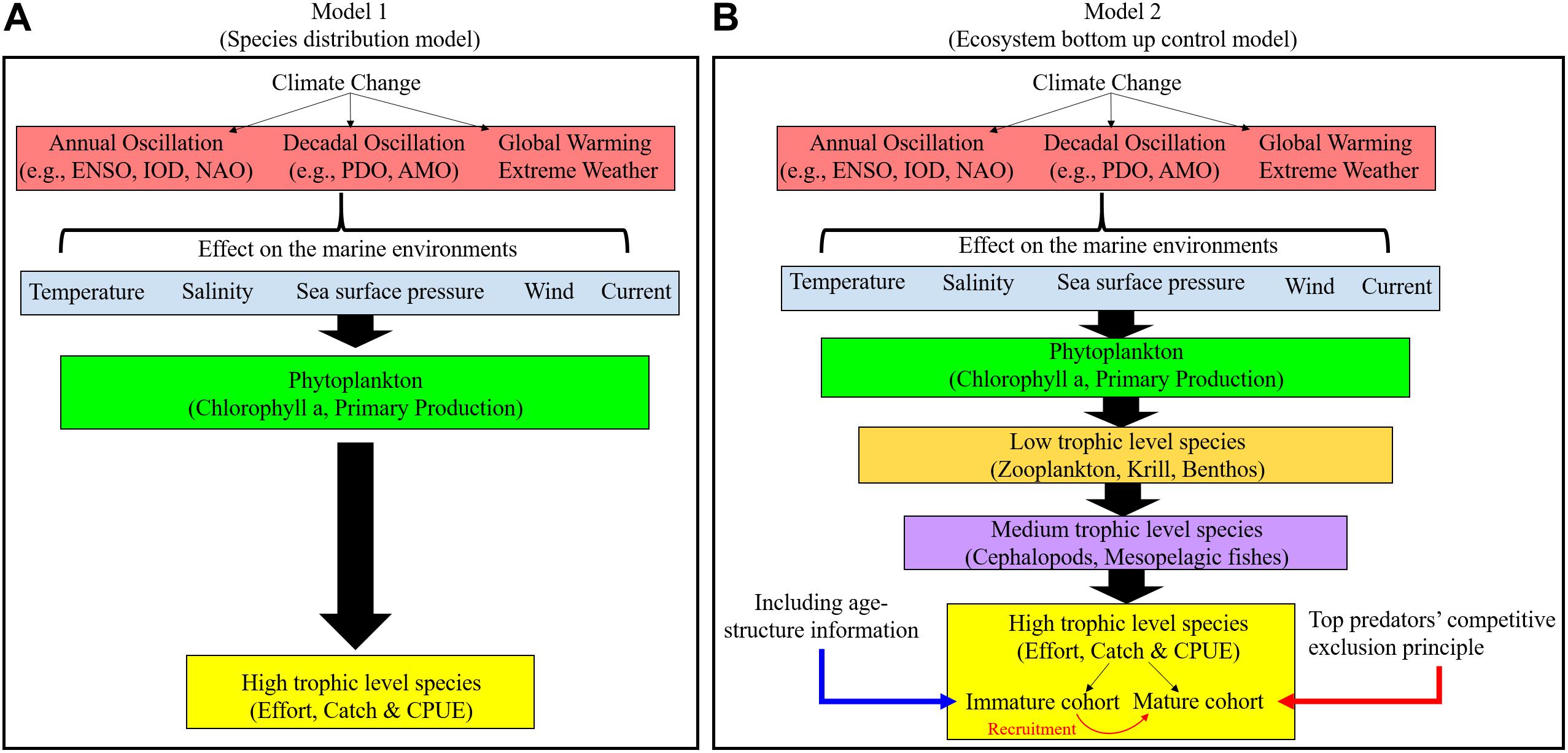
Figure 1. Flow of data processing and analyses used in (A) Species distribution models and (B) Ecosystem bottom-up control models to understand the influence of climate change on top predators.

At present, we have a poor understanding of the climate change-induced processes that alter the distribution of top predators, particularly in terms of amplitude and lagged processes (Corbineau et al., 2008; Hsieh et al., 2008; Botsford et al., 2011; Lan et al., 2013, 2019; Nieto et al., 2017). These processes have been difficult to determine because fluctuations in top predator populations are explained by a non-linear combination of factors (environmental and otherwise) rather than a single factor; these factors pertain to, for example, fishing efforts, targeting practices, and fleet dynamics (Hsieh et al., 2008; Tu et al., 2018). Furthermore, the high mortality rates of mature fish are caused by factors (e.g., exploitation) that can ultimately alter how fish populations respond to their physical environment (Rouyer et al., 2012; Tu et al., 2018).

The movements and distributions of top predators are conditioned through bottom−up processes and through direct environmental effects (e.g., physiological tolerance to anoxia and thermal preferences). Time lag results elucidate the delay in the response of a dependent variable to a stimulus (Borges et al., 2003). The time and area strata that are favorable for spawning and feeding are limited and variable (Fonteneau and Soubrier, 1996; Fonteneau et al., 2008). Therefore, changes in species density occur after fluctuations in the dynamics of an interacting species or of a limited resource (Borges et al., 2003). Thus, most tuna species develop thermoregulation capabilities, and the efficiency of thermoregulation is variable and dependent on size (Holland et al., 1992; Fonteneau and Soubrier, 1996). Tropical-temperate tuna species [e.g., bigeye tuna (BET)] and temperate tuna species (e.g., bluefin tunas) migrate extensively between their spawning areas and feeding grounds (Fonteneau and Soubrier, 1996; Fonteneau et al., 2008). Specifically, the growth and survival rates of juvenile and immature cohorts depend on mechanisms that control the local food supply within their favored habitats (Bakun, 2006). Thus, through understanding how low-trophic marine ecosystems relate to each life stage of top predators, we can better understand how climate change influences the distribution and abundance of top predators (Figure 1B).

Although predictions of the climate change-induced habitat shifts of top predators have improved, the abundance and distribution of top predators at each life stage in marine ecosystems remain relatively unknown. This study used BET as a case study. BET has a lifespan of >10 years; the age at first maturity is 2–3 years, and spawning occurs in warm tropical waters (Lehodey et al., 2010). Based on Taiwanese longline fishery data, this study investigated the temporal and spatial variations in the fishing grounds and catch per unit effort (CPUE) of immature and mature BET cohorts in the western and central Pacific Ocean (WCPO, the area west of 150°W).

In the North Pacific Ocean, BET primarily preys on organisms in the fish and squid taxa (Ohshimo et al., 2018). Thus, we first analyzed the long-term data on the crucial pelagic species of Pacific saury and neon flying squid (trophic level: 2–4); second, we determined the abundance of eggs and larvae for these species (trophic level < 2). Wavelet analysis is a common tool for time series analysis, and it involves decomposing a time series into time and frequency components; this helps the analyst to identify the dominant periodic components and to determine how these components vary over time (Torrence and Compo, 1998; Wu et al., 2020). Specifically, in this study, we used wavelet analysis to further explore the processes underlying the bottom-up control of the pelagic ecosystem, where these processes are influenced by decadal climate events in the WCPO.

Materials and Methods

Fishery Data and Age Structure of Bigeye Tuna

We analyzed 1994–2014 data from the logbooks of Taiwanese longline fleets, which were provided by the Overseas Fisheries Development Council of the Republic of China. The fishery data, which were recorded in 5° spatial grids, pertained to fishing effort (indicated by number of hooks), fishing date, catch amount (number of fish caught for each species), and fork length (randomly sampled and measured in centimeters). However, fork length had fewer data points (<3000 fish) with a lower spatial coverage for before 2002; the number of data points was >10⁴ fish caught during 2002–2014. Thus, the 2002–2014 fork length data were used to estimate the mean values of fork length by age.

The flowchart in Figure 2 illustrates how we processed the fishery and age structure data. The fork length at maturity is defined as the length at which 50% of females are mature (L50), which for BET in the WCPO is estimated to be 103 cm (Farley et al., 2017). We therefore distinguished immature (<103 cm) from mature (≥103 cm) cohorts and calculated the monthly percentages of immature and mature cohorts in each grid.

FIGURE 2

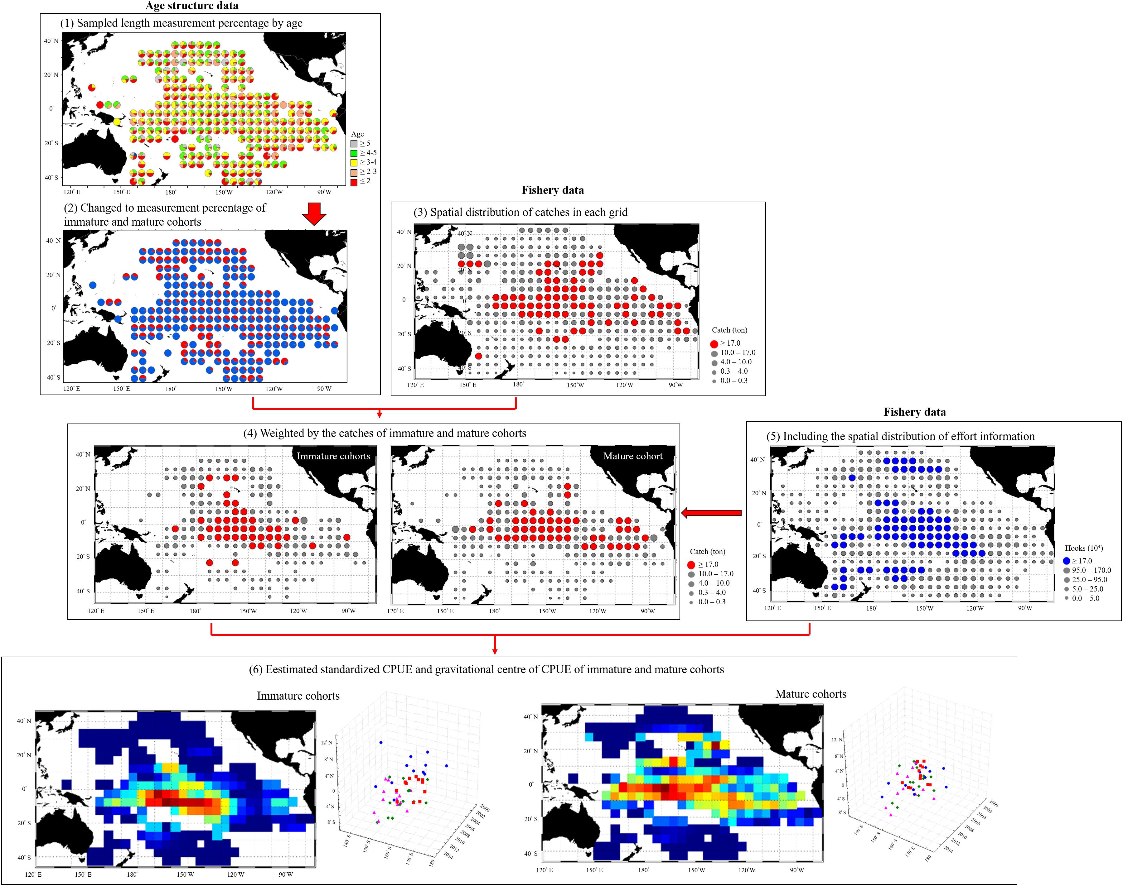
Figure 2. Flow chart of processing and analysis of fishery and age structure data.

The catch numbers of the two cohorts by species were weighted by the spatial distributions of catch data. To better understand the spatial distribution of the fishery and the associated variability, we estimated the nominal CPUE to be the number of fish captured per 1000 hooks (individuals/10³ hooks); subsequently, we determined the gravitational center of CPUE (G) based on the nominal CPUE and seasonal location of fishing vessels (L) through the following formula.

$${\text{G}}_{latitude}=\frac{\sum {\text{L}}_{\text{i}}\times \mathrm{nominal}{\mathrm{CPUE}}_{\text{i}}}{\sum \mathrm{nominal}{\mathrm{CPUE}}_{\text{i}}}(1)$$

$${\text{G}}_{\text{longitude}}=\frac{\sum {\text{L}}_{\text{j}}\times \mathrm{nominal}{\mathrm{CPUE}}_{\text{j}}}{\sum \mathrm{nominal}{\mathrm{CPUE}}_{\text{j}}}(2)$$

where i and j denote the latitude and longitude, respectively, of individual fishing locations in the 5° grid.

Standardization of Nominal CPUE

The nominal CPUE had to be standardized because it can vary substantially in time and space with respect to targeting practices, such as the targeting of albacore or BET by fishers, which is principally driven by market trends and gear efficiency (Lan et al., 2013; Wu et al., 2020). We standardized the nominal CPUE values of BET cohorts by using generalized linear models (GLMs). The main variables were temporal (year and month) and spatial (longitude and latitude) variables, the catch rates of albacore, and interaction terms for two covariates. The GLMs had the following general form:

$$\mathrm{Log}(\mathrm{CPUE}+\mathrm{c})=\mathrm{\mu }+year+month+latitude+\mathrm{longitude}+\mathrm{albacorecatchrates}+\mathrm{Interactions}+\mathrm{\epsilon }(3)$$

where CPUE is the nominal CPUE (individuals/103 hooks) of BET cohorts, μ is the intercept, and ε is a normally distributed variable with a mean of 0. Because the log-link function cannot handle zeros, 10% of the overall mean of nominal CPUE was added before the logarithm function to ensure that the result was a rational number (Lan et al., 2013; Wu et al., 2020). The best model was selected based on the residual deviance, and the Akaike information criterion decreased as more variables were added. Time and location were treated as interaction terms to account for possible monthly and interannual variability driven by climatic variations in the spatial distribution of BET cohorts. Furthermore, in our analyses, we used generalized additive models (GAMs) to investigate the effects of the interaction terms; GLMs and GAMs were executed in R (Version 2.15.0) using the mgcv package.

Data From Purse Seine, Pacific Saury, and Neon Flying Squid Fisheries and on Egg and Larva Abundance

The immature cohort of BET in this study was also identified from surface schools with other tuna species (e.g., skipjack and yellowfin tuna) that were caught using purse seine nets (Lehodey et al., 2010; Ducharme-Barth et al., 2020). Although this cohort is essentially a bycatch of BET in purse seine fisheries, the catch volume was substantial at approximately the same order of magnitude as that for longline fisheries, and the fish that were caught were mainly from the immature cohort of BET (Ducharme-Barth et al., 2020). Thus, we further downloaded 1995–2016 purse seine fishery data from the Western and Central Pacific Fisheries Commission website. The technology behind fixed and free-floating fish aggregation devices has continually improved; they have influenced the behavioral and movement patterns of juvenile and small-size tuna (Leroy et al., 2013). Therefore, BET abundance may be more accurately indicated by BET catch rates as obtained from natural logs. Thus, the natural-log schools of BET were selected, and the catch rates were calculated in terms of the weight of fish captured daily (tons/day); this revealed the time series patterns of the immature cohort.

Fisheries data of neon flying squid were downloaded from the website of the North Pacific Fisheries Commission¹. The 1995–2016 Japanese fishery data used in this study were included the number of vessels, fishing days, fishing areas (west and east of 170°E and the northwestern Pacific Ocean), and catch (measured in metric tons). We calculated the average annual catch rates of neon flying squid in the North Pacific Ocean. As shown in Figure 3B, the biomass of Pacific saury in the North Pacific Ocean of this study was obtained from the fourth meeting report of the technical working group assessing the stock of Pacific saury (Figure 3A of NPFC, 2019).

FIGURE 3

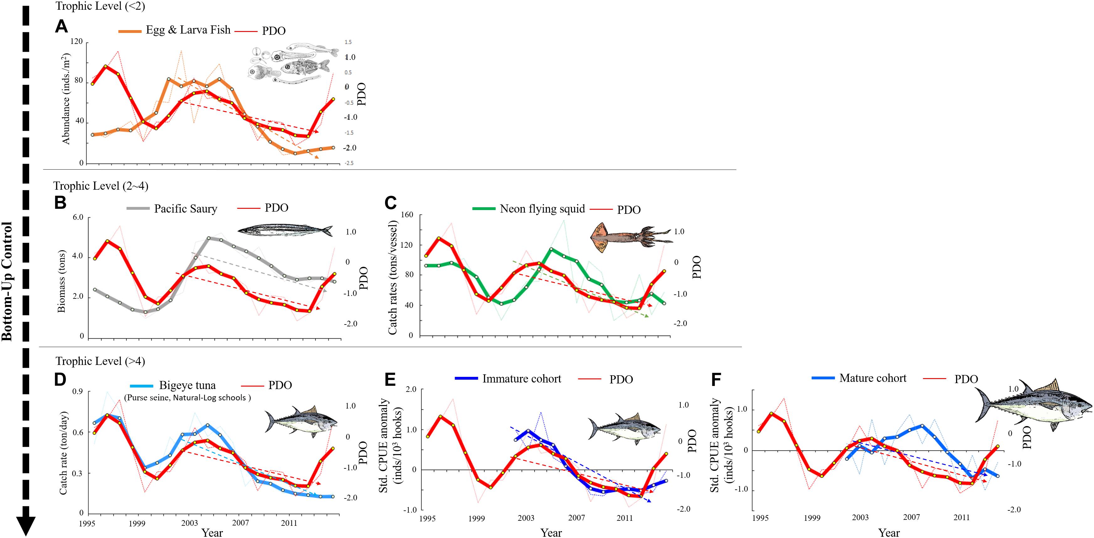
Figure 3. Annual (thin dotted line) and 3-year mean (thick solid line) trends of the pelagic ecosystem for species with low trophic (<2) to high trophic (>4) levels as influenced by PDO in the WCPO. (A) Abundance of eggs and larvae, (B) biomass of Pacific saury, (C) catch rates of neon flying squid, (D) catch rates of nature-log schools of BET caught in purse seine nets, and (E,F) standardized CPUE anomaly of immature and mature cohorts of BET. The dashed lines in (A–E) indicate that the phases have significant correlations with the interannual pelagic ecosystem and PDO in a Pearson’s test.

Data on the abundance of eggs and larvae were for ichthyoplankton biomass; these data were gathered by a group dedicated to studying coastal and oceanic plankton². The CalCOFI dataset was established through long-term and uninterrupted sampling of larvae and eggs in the region bounded by 20°N–51°N and 106°W–146°W.

Interannual and Decadal Climatic Variability Indices

The El Niño/Southern Oscillation (ENSO) and Pacific Decadal Oscillation (PDO) are well-known and dominant manifestations of interannual and decadal global climate change that develop from air–sea interactions in the Pacific Ocean (Mantua and Hare, 2002; Bell et al., 2011). In this study, the ENSO was represented by the Oceanic Niño Index (ONI) and was estimated by a 3-month running mean of sea surface temperature anomalies in the Niño 3.4 region (5°N–5°S, 120°W–170°W) between 1986 and 2015. The ONI is the most common index for measuring and defining El Niño and La Niña events, and other indices (e.g., Niño 1 + 2, 3, and 4) can verify whether these periods are accompanied by features that are consistent with a coupled ocean–atmosphere phenomenon (Glantz and Ramirez, 2020). This study represented the PDO by the first empirical orthogonal function (EOF1) in an analysis of temperature anomalies in the detrended sea surface north of 20°N in the Pacific Ocean (Mantua and Hare, 2002), and data on the PDO data were downloaded from the NOAA Earth System Research Laboratory.

Cross-Wavelet Coherence and Phase Analyses

This study used wavelet analysis to investigate how environmental variations caused by the interannual and decadal climate events of the ENSO and PDO affected the temporal standardized CPUE of immature and mature cohorts. Fourier spectral analysis is commonly used to analyze periodicities in time series data, but this approach assumes that the time series is stationary. The time series of climatic indices and fishery data were not stationary. Thus, we used wavelet analysis because it requires no such assumption (Wu et al., 2020). The wavelet transformation is based on a convolution between a time series y_n (n = 0,…, N − 1, with equal spacing δt) and a wavelet function. The Morlet wavelet is the most popular complex wavelet used in practice and is defined as

$${\mathrm{\psi }}_0(\mathrm{\eta })={\mathrm{\pi }}^{-1/4}{e}^{i{\mathrm{\omega }}_0\mathrm{\eta }}{e}^{-\frac{1}{2}{\mathrm{\eta }}^2}(4)$$

where η is a dimensionless time parameter and ω₀ is a dimensionless frequency used to balance time and frequency localization. The wavelet transform of y_n is

$${\text{W}}_{\mathrm{n}}^{\text{y}}(s)=\sqrt{\frac{\mathrm{\delta }t}{s}}\sum _{n^{\prime }=1}^N{y}_{n^{\prime }}{\mathrm{\psi }}_0\left[(n^{\prime }-n)\frac{\mathrm{\delta }t}{s}\right](5)$$

where s is a scale such that η = st. By varying s, the wavelet is extended through time. A 5% significance level was set based on 1000 bootstrap simulations with a spectral synthetic test (Rouyer et al., 2008). The autoregression coefficient was empirically obtained from the time series data. Subsequently, cross-wavelet coherence and phase analyses were used to investigate the relationships between PDO events and the pelagic ecosystem in the WCPO.

Cross-wavelet coherence and phased analyses represent cross-correlations normalized to the power of a single process and are thus not biased by the power of any single series (Grinsted et al., 2004). We defined the cross-wavelet transformation of the two series x_n and y_n to be ${\text{W}}_{}^{\text{XY}}={\text{W}}_{}^X{\text{W}}_{}^{Y^{*}}$, where ^∗ denotes a complex conjugation. The wavelet coherency was defined as

$$R_{\text{n}}^2(s)=\frac{{\left|S(s^{-1}{\text{W}}_{\mathrm{n}}^{XY}(s))\right|}^2}{S(s^{-1}{({\text{W}}_{\mathrm{n}}^X(s))}^2\cdot S{(s^{-1}{\text{W}}_{\mathrm{n}}^Y(s))}^2}(6)$$

where S is a smoothing operator determined based on a running average.

The wavelet coherency phase is

$${\mathrm{\varphi }}_{\text{n}}(s)={\tan }^{-1}\left(\frac{Imaginary\left\{S\left(s^{-1}{\text{W}}_{\mathrm{n}}^{XY}\left(s\right)\right)\right\}}{Real\left\{S(s^{-1}{\text{W}}_{\mathrm{n}}^{XY}(s))\right\}}\right)(7)$$

where both $R_{\text{n}}^2(s)$ and φ_n(s) are functions of the time index n and scale s. Torrence and Compo (1998) and Grinsted et al. (2004) have detailed the mathematics underlying this analysis. The wavelet transform has edge artifacts because the wavelet is not completely localized in time, and the finite nature of such images gives rise to edge artifacts in the reconstructed data. Therefore, a cone of influence can be introduced where edge effects cannot be ignored (Grinsted et al., 2004).

Results

Distribution of Immature and Mature BET Cohorts

The catch percentage of the Taiwanese longline fisheries in the WCPO indicated that most BET catches were from the mature cohort (approximately 81%, Figure 4A). The immature cohort comprised approximately 18–35% of the total catch between 2002 and 2006, and this proportion decreased to approximately 8% in 2009. To combine the spatiotemporal length–frequency and logbook data for 5° spatial grids (Figures 4B–D), we further calculated the distribution and gravitational center positions of the nominal CPUE of immature and mature cohorts (Figure 5). The seasonal spatial distribution suggested that the immature cohort was concentrated in subtropical waters (20°N–30°N) during the first quarter before gradually moving southward to tropical waters (Figures 5A,B). The mature cohort was concentrated in tropical waters throughout the year (Figures 5C,D).

FIGURE 4

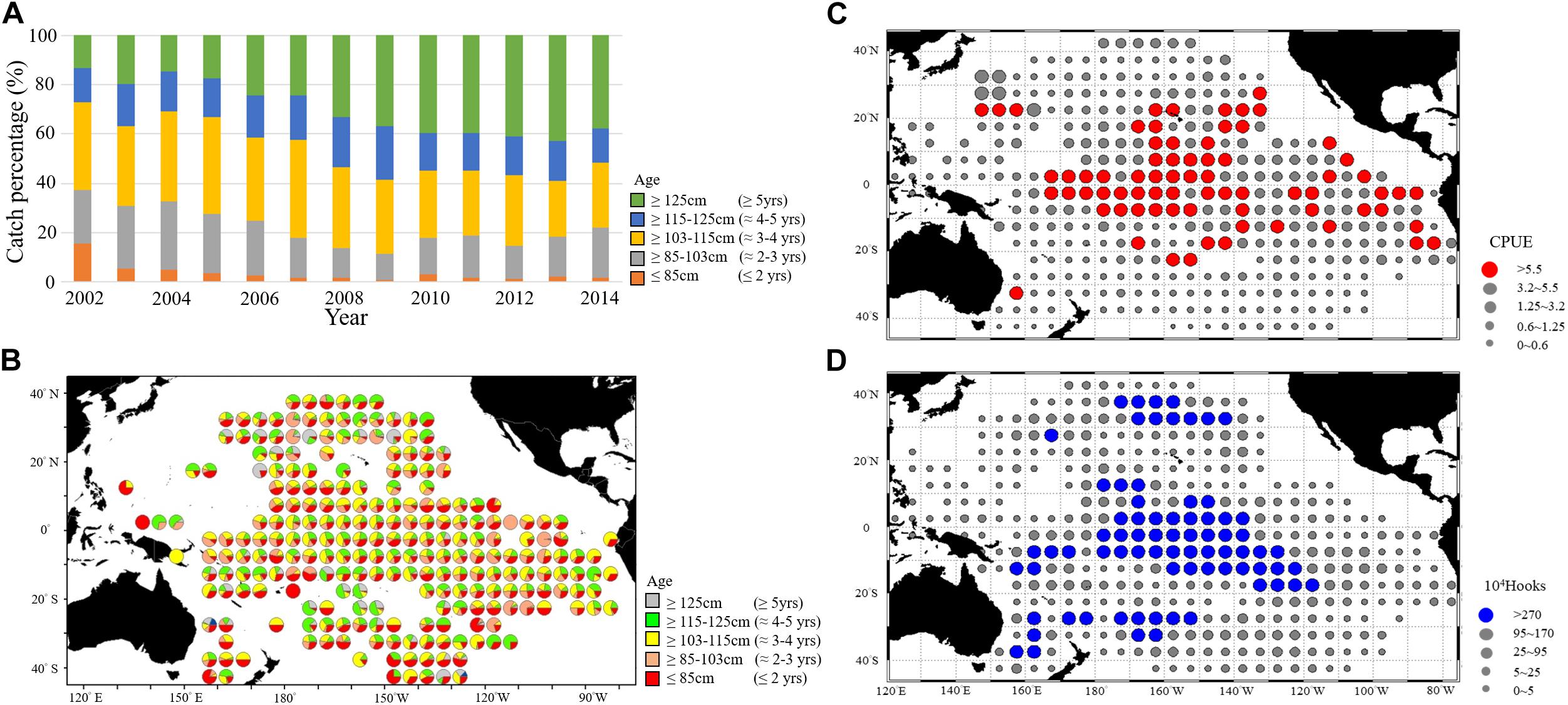
Figure 4. (A) Annual trends of BET catch percentage for various age ranges. Spatial distributions of (B) Catch percentage of BET for various age ranges, (C) Nominal CPUE of BET, and (D) Effort in 5° spatial grids during the entire study period.

FIGURE 5

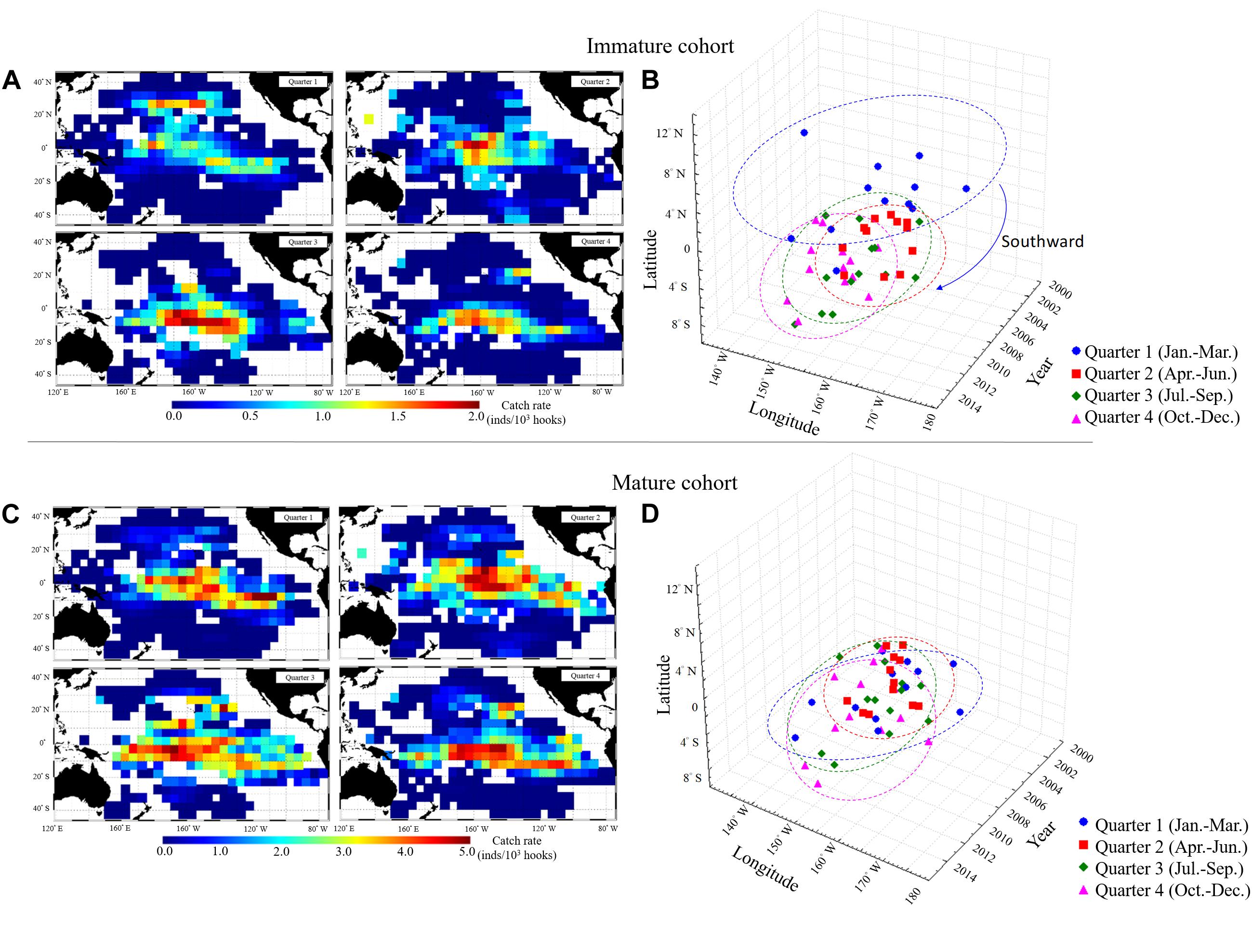
Figure 5. Seasonal spatial distributions of average nominal CPUE in 2002–2014 for (A) Immature and (B) Mature BET cohorts. Seasonal gravitational center positions over years of the catch rates (quarters 1–4) in each year for (C) Immature and (D) Mature BET cohorts in the WCPO.

Time Series Analysis of the Standardized CPUE of BET and Climate Events

Before the time series analysis was conducted, nominal CPUE values were standardized by using GLM; the model selection criteria are shown in Table 1. The selection of GLMs for analysis revealed that temporal factors, spatial factors, and the two interaction terms of (1) latitude with year and (2) month with longitude were significant for the immature and mature cohorts. However, the catch rate of albacore was not significant for the mature cohort. Furthermore, the deviance explained by the selected GAMs was 46.40 and 71.70% for the immature and mature cohorts, respectively. The results for the interaction terms in the GAM indicated that the immature cohort had a high CPUE in tropical and subtropical waters (Figure 6A, 20°S–40°N, 160°E–160°W) during the first half of the year (Figure 6B). However, the CPUE decreased after 2006 in subtropical waters (Figure 6C). The mature cohort tended to have a high CPUE in tropical waters (Figure 6E, 20°S–20°N, 160°E–110°W) throughout the year (Figure 6F), but the CPUE also decreased after 2009 in tropical and subtropical waters (Figure 6G). In addition, the standardized CPUE of both the mature and immature cohorts decreased over time in subtropical waters (north of 20°N) after 2006 and 2009, respectively (Figures 6D,H).

TABLE 1

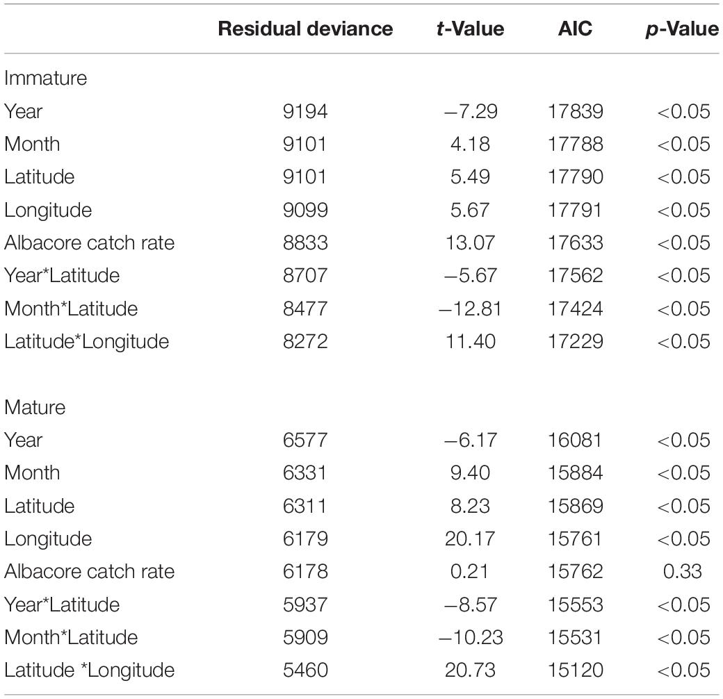
Table 1. GLM, residual deviance, approximate Akaike information criterion, and p-values for GAM models of immature and mature cohorts of BET in the WCPO.

FIGURE 6

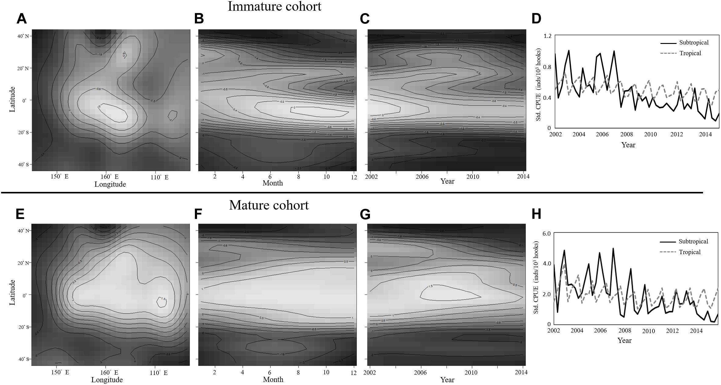
Figure 6. GAM results for the effects of three interaction terms, namely (A,E) Longitude with latitude, (B,F) month with latitude, and (C,G) Year with latitude, on CPUE for immature (A–D) and mature (E–H) BET cohorts. Quarterly standardized CPUE in the subtropical (black line) and tropical (gray line) WCPO for (D) Immature and (H) Mature BET cohorts.

By using state-space time series analysis and a single decomposition procedure, we removed seasonality from the time series dataset, which comprised data on climatic indices and data from the standardized CPUE dataset. The cross-wavelet coherence results indicated a significant positive correlation (in-phase arrows in Figure 7) between standardized CPUE and ONI in both cohorts, with periodicities of approximately 2 years during 2002–2006 and 2010–2014 (Figures 7A,B). Standardized CPUE was significantly and positively related to PDO in the immature cohort throughout the study period (Figure 7C); however, it was negatively correlated with PDO (out-of-phase arrows in Figure 7), with intermittent periodicities, in the mature cohort (Figure 7D).

FIGURE 7

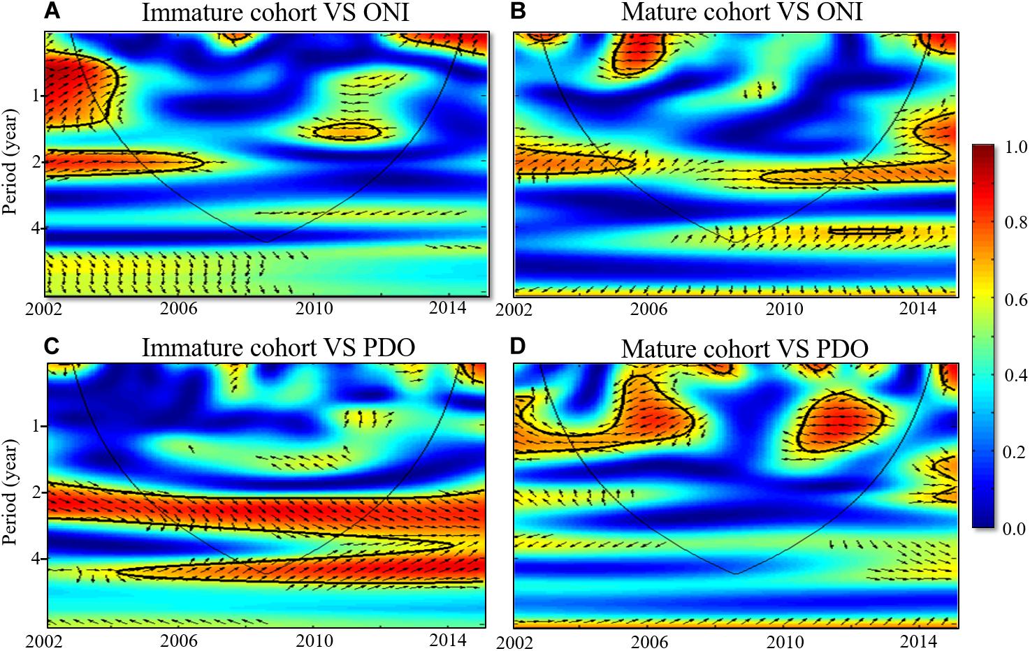
Figure 7. Cross-wavelet coherence between monthly standardized CPUE of (A,C) Immature and (B,D) Mature BET cohorts with ONI and PDO from 2002 to 2014. Black solid contours enclose regions with > 95% confidence, and the black line indicates areas where edge effects are significant. High and weak variabilities are represented by red and blue colors, respectively. Arrows indicate the phase relationships, with in-phase arrows (positive correction) pointing to the right and out-of-phase arrows (negative correction) pointing to the left.

Bottom-Up Control of the Pelagic Ecosystem Under the Effects of Decadal Climate Events

The wavelet analysis results highlighted the different periodicities between BET cohorts and PDO. The catch rate of natural-log schools of BET was also strongly positively correlated with PDO, with a periodicity of approximately 8 years between 1995 and 2014 (Figure 8A). The GAM results revealed that the standardized CPUE of both mature and immature cohorts decreased over time in subtropical waters (north of 20°N) after 2006 and 2009, respectively. The food web was affected by bottom-up climate change through changes in physical factors. Thus, the abundance of the BET prey of Pacific saury and neon flying squid (trophic level: 2–4) and the abundance of their eggs and larvae (trophic level < 2) in the region north of 20°N were selected for further analysis. Wavelet analysis was used to further investigate the effects of PDO on the abundance of neon flying squid, Pacific saury, eggs, and larvae in the WCPO. Strong positive correlations were identified between the abundances of eggs and larvae, Pacific saury, and PDO, with periodicities of approximately 8 years between 1995 and 2014 (Figures 8B,C). Moreover, the time lags were observed between the abundances of neon flying squid and PDO with 1–2-years (Figure 9A), and also had periodicities of approximately 8 years between 1995 and 2014 (Figure 8D). The evolution of the abundances of eggs and larvae, Pacific saury, and neon flying squid, with a 1–2-year lag, were similar to that of PDO (Figures 3A–C). The catch rate of natural-log schools of BET caught by purse seine nets decreased from 1998 to 2004, as did the PDO (Figure 3D). The standardized CPUE anomaly of immature cohorts decreased from 2004 to 2012 (Figure 3E), and that of mature cohorts increased from 2003 to 2008 before decreasing from 2009 onward (Figure 3F). The annual values of standardized CPUE in the immature cohort evolved in a similar manner as the abundances of eggs and larvae, Pacific saury, and neon flying squid and the catch rate of BET caught by purse seine nets. In general, the values of the variables increased from 2000 to 2004 and decreased thereafter until 2012 (Figure 3). Furthermore, the mature cohort had a standardized CPUE anomaly that lagged behind that in the immature cohort by 3 years (Figure 9B).

FIGURE 8

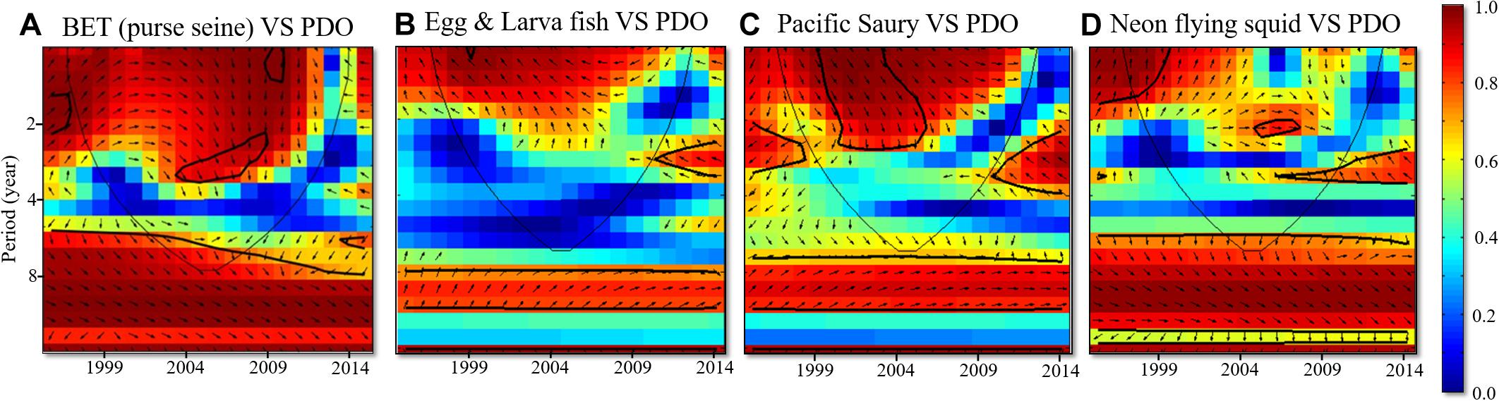
Figure 8. Cross-wavelet coherence between (A) Catch rates of nature-log schools of BET caught using purse seine nets, (B) Abundances of eggs and larvae, (C) Biomass of Pacific saury, and (D) Catch rates of neon flying squid influenced by PDO from 1996 to 2014. Refer to Figure 7 for additional details.

FIGURE 9

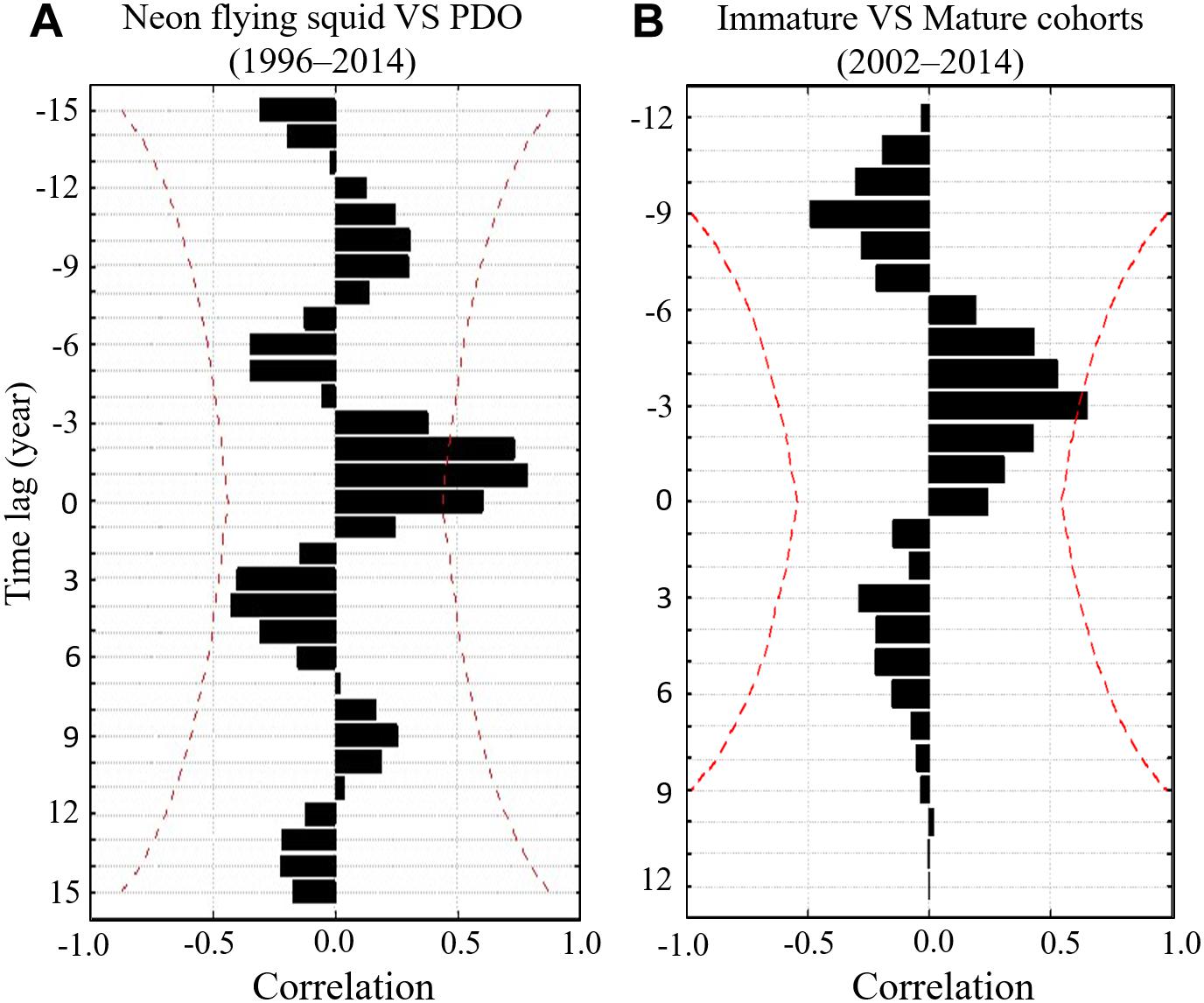
Figure 9. Cross-correlation function between (A) Annual catch rates of neon flying squid and PDO in 1996–2014 and (B) Annual standardized CPUE of immature and mature cohorts of BET in 2002–2014. Two red dotted lines represent the limits of significance at the 5% level.

Discussion

Bigeye tuna is a highly valuable species that faces overfishing pressure because of the prevalence of longline subsurface fisheries and because BET is a bycatch of purse seine surface tuna fisheries (Lehodey et al., 2010). Catch rate and fork length data for the 2002–2014 period from Taiwanese longline fleets were used in this study. The Taiwanese longline fleet began operating in the mid1960s and mainly targeted the albacore in the south Pacific Ocean. The historical catch information and logbook data for Taiwanese longlines in the Pacific Ocean have been available since 1964, and the spatiotemporal length-frequency data have been available since 1981 (Wang et al., 2009). Since the late 1990s, many Taiwanese longline fleets have been equipped with supercold storage equipment and have targeted BET and yellowfin tuna using deep longlines (Lan et al., 2012b; Wu et al., 2020). The development of BET fisheries through the use of deep longline vessels since 2002 has resulted in more catches, and the annual length-frequency sample sizes of the data increased from approximately 500–3000 fish before 2000 to more than 10⁴ fish in recent years (Wang et al., 2009). This meant that before 2002, the data only revealed sporadic and incomplete information on the spatiotemporal distribution of BET cohorts.

Large-scale migration frequently occurs between spawning and feeding grounds, covering hundreds or thousands of miles, as has been clearly demonstrated for BET in the Atlantic Ocean and Pacific Ocean (Fonteneau and Soubrier, 1996; Hallier et al., 2005). We combined spatiotemporal data from the Taiwanese longline fishery with data on fork length, which had a spatial resolution of 5°. We noted that for the immature cohort, a region with high CPUE values moved southward from temperate to tropical waters during the first quarter of each year; such southward movement was also noted in the WCPO more generally. BET caught using purse seine nets were also mainly from the immature cohort in the tropical waters of the Pacific Ocean. Mark-and-recapture data revealed that the BET migration differed depending on the age group and ranged from 1000 to 3000 nautical miles (Schaefer et al., 2015). BET is highly prone to year-round migration and spawning in tropical waters (Miyabe, 1994). The GAM results also showed that CPUE tended to be high for the immature cohort in tropical and subtropical waters and high throughout the year for the mature cohort in tropical waters.

However, Schaefer et al. (2015) analyzed extensive tagging data and observed that the movement of immature BET was constrained latitudinally in the equatorial central Pacific Ocean, rarely extending to higher latitudes. To further investigate how BET migrated across its life cycle in the WCPO, we overlaid the distributions of the immature and mature cohorts from the longline fishery data of this study and the distributions of larvae and adult habitats, as reported by Reglero et al. (2014), on top of the major surface currents in the tropical and subtropical Pacific Ocean (Figure 10). The immature and mature cohorts were observed across the equatorial Pacific Ocean with respect to the equatorial current system (Figure 10, mature cohort and adult habitat). The equatorial current system is the foundation for the highly productive equatorial upwelling that supports high concentrations of mesopelagic fish, cephalopods, and crustaceans (Schaefer et al., 2015).

FIGURE 10

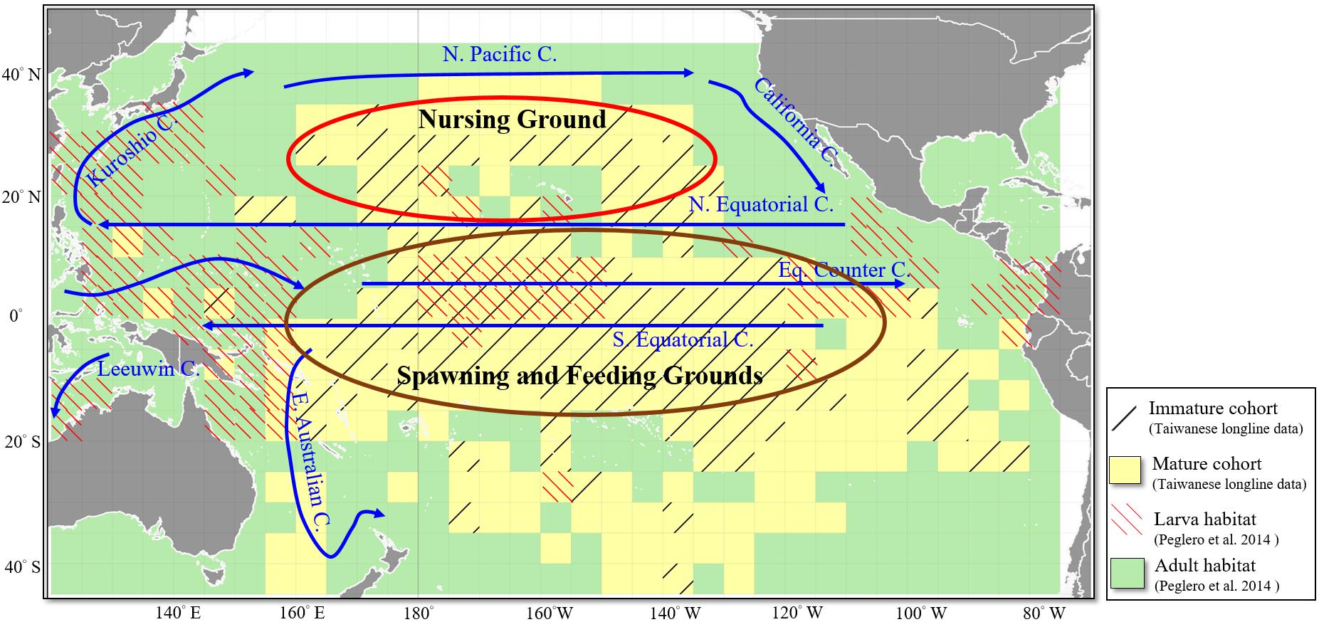
Figure 10. Distribution of the immature and mature cohorts of BET (black slash line and yellow grids) revealed in this study and the larva and adult habitats (red slash line and green grids) revealed by Reglero et al. (2014) overlaid with the major surface currents (blue lines) in the tropical and subtropical Pacific Ocean. The red and brown ellipses indicate the possible nursing, spawning, and feeding grounds for different life stages of BET.

In addition, the immature cohort was found to have a high CPUE in subtropical waters Tuna larval habitat is related to the occurrence of mesoscale oceanographic activity (Bakun, 2006). BET larvae were present in the tropical WCPO along the Kuroshio current to the Japanese coast (Reglero et al., 2014). We further speculated that equatorial counter currents transport the eggs and larvae of BET to the eastern and western coastal waters and then to the temperate waters in the north (Figure 10, larva habitat and immature cohort). Studies have suggested that BET caught in tropical Pacific waters tend to be more sexually mature than those encountered in temperate waters. Because temperate waters are too cold, BET in these regions may not reach sexual maturity or their gonads may not be ready for reproduction (Miyabe, 1994). Fronts are narrow bands with horizontal gradients that indicate regions demarcated by physical, chemical, and biological differences, which can be used to divide the ocean into various water masses; predators aggregate around the fronts where their preferred prey gather (Olson et al., 1994; Lan et al., 2012a). Further studies that consider oceanic fronts as aggregating mechanisms and as mechanisms that limit the distribution of BET cohorts will further elucidate the factors influencing the spatial distribution of BET in the WCPO.

El Niño/Southern Oscillation events are associated with changes in the equatorial trade winds and the corresponding major currents in the basin, resulting in shifts in the equatorial warm pool region (Izumo et al., 2010; Bell et al., 2011). The effects of ENSO-related changes in thermal structure have been clearly associated with the vertical extension of the tuna habitats in the Pacific Ocean (Lehodey et al., 2010; Bell et al., 2011, 2013). The PDO, the most prominent decadal variability in the North Pacific Ocean, is characterized by a horseshoe-shaped pattern in sea surface temperature anomaly (Li et al., 2020). The PDO has changed its phase several times since the 1900s, and these regime shifts substantially influence current, temperature, and primary production. Consequently, epipelagic forage controls the habitats and dynamics of larvae and juvenile organisms (Miller and Schneider, 2000; Newman et al., 2016). The immature BET cohort was found in surface schools with other tuna species; adult fish explore deeper layers where they can find mesopelagic prey species (Lehodey et al., 2010). Thus, this substantial oceanographic phenomenon likely induced changes in positions and thermal environments in the subtropical fronts, which would have affected the migrations of the forage that immature BET cohort prey on; these prey include mesopelagic fish, such as Pacific saury and neon flying squid.

Because of the fluctuating global mean temperature, the phase shift of the PDO at the end of the 20th century has been considered an influential factor affecting the recent hiatus in surface warming (Kosaka and Xie, 2013; Li et al., 2020). However, the planet’s warming climate has shortened PDO periodicity because of the acceleration of Rossby waves and the decrease in PDO amplitude through a reduction in its development time (Li et al., 2020). The changes in the abundances of Pacific saury and neon flying squid revealed an interannual-decadal pattern of variation with regime shifts in large-scale climatic indices (Igarashi et al., 2017; Yu et al., 2017; Liu et al., 2019). The PDO may be a major factor for differentiating physical processes and subsequent responses in the zooplankton community structures (Chiba et al., 2015). The copepod community size has increased after 2006 and 2007 in the North Pacific Ocean because of the increased dominance of large cold-water species (Chiba et al., 2015). Olson et al. (2014) revealed a major decadal-scale dietary shift in yellowfin tuna over a broad region of the eastern Pacific Ocean, suggesting that more broad-scale food web changes had occurred in lower trophic levels in the 2000s than in the 1990s. The stock assessment estimates provided by Ducharme-Barth et al. (2020) also indicated a decrease over time in estimated spawning potential and in the recruitment of BET within the WCPO.

The present results also revealed crucial synchronous shifts in the effect of the pelagic ecosystem at low trophic levels on the immature BET cohort (including the nature-log schools of BET caught by purse seine), with a decreasing trend after 2004–2005 caused by the PDO. The results suggested that the PDO’s decadal climate index affected the pelagic ecosystem due to the low trophic levels of eggs and larvae; this effect has progressed to small pelagic fish, cephalopods, and the top predators of the immature BET cohort, acting as a bottom-up control regulator. The feeding habits of BET also revealed that larger BET preyed on larger fish—their prey ranged from the smaller Eucleoteuthis luminosa to the larger Magnisudis atlantica—and indicated ontogenetic shifts in the feeding habits of BET in the North Pacific Ocean (Ohshimo et al., 2018). Thygesen et al. (2016) also suggested that BET diving behavior while foraging varied with body size due to ontogenetic changes in physical and physiological characteristics (e.g., swimming speed and the development of endothermy). Furthermore, in the WCPO, the decrease in food stocks for the immature BET cohort may have decreased recruitment into the mature cohort after 3 years, as indicated by the 3-year lag in our results. This finding confirmed that the age structure of top predators can be critical for predicting the responses of populations to species interactions at both the micro and macro ecological scales under the influence of climate change. Declines in the abundance of forage fish resulting from heavy fishing pressure and changes in the marine environment have been observed worldwide (Olson et al., 2014; Madigan et al., 2016; Liu et al., 2019), and an understanding of predator–prey relationships has become crucial to managing fisheries.

Bigeye tuna recruitment may occur throughout the year because individual fish can spawn almost every day if the marine environment (e.g., water temperatures) is suitable (Kume, 1974). However, variability in early growth influences the stage at which young fish are vulnerable to predation, which, in turn, influences the accumulated mortality during early life stages and recruitment to the population (Houde and Hoyt, 1987). The present study did not apply complex ecosystem models in response to the general concern regarding the combined effects of fishing and climate. Instead, the actual spatial distribution of the age structure of BET was used to investigate the time series relationship between the pelagic ecosystem and decadal climatic index in the potential BET nursing ground. When analysts assess the impact of climate change, because of computational constraints, they typically use ecosystem models that are of an approximated or simpler form in their representation of age structures and spatiotemporal variations (Botsford et al., 2011; Glaser et al., 2014). If information on age structure and spatiotemporal variation is absent, then ecosystem models may not adequately depict the variability attributable to cohort resonance and long-term changes in abundance (Botsford et al., 2011).

Top marine predators can have high phenotypic plasticity and adaptive capabilities that mitigate the effects of climate change on them; however, climate change may still affect these predators through their prey (Hazen et al., 2013). Our analysis only applied to a top predator, BET, in the WCPO. Nevertheless, we provided evidence that the true spatial distribution and time series variation of age structures are important indices for investigating the effects of climatic events on pelagic ecosystems. However, many top predators in marine ecosystems adopt different life strategies and we did not investigate the potential effects of the interactions between climate change and other human stressors. Future studies should use ecosystem models that describe the full population age structure from larvae through to the mature stock (e.g., SEAPODYM models, Lehodey et al., 2010). Furthermore, to better elucidate how species are threatened by climate change, future studies should extend their spatiotemporal time series data on fishery and age structure by including data on a diversity of gear types and fishing strategies.

Data Availability Statement

The raw data supporting the conclusions of this article will be made available by the authors, without undue reservation.

Author Contributions

K-WL led the study design and wrote the article. Y-LW and T-HL contributed materials of GAM and wavelet analysis. L-CC and MN contributed for fisheries data collected and data analysis. All authors read and agreed to the published version of the manuscript.

Funding

This study was financially supported by the Council of Agriculture (107AS-9.1.5-FA-F1 and 108AS-9.2.1-FA-F1) and the National Science Council (MOST 107-2611-M-019-017 and MOST 108-2611-M-019-007).

Conflict of Interest

The authors declare that the research was conducted in the absence of any commercial or financial relationships that could be construed as a potential conflict of interest.

Acknowledgments

We are grateful to the Overseas Fisheries Development Council (OFDC) of Taiwan for providing data from the Taiwanese longline fishery. We also thank the North Pacific Fisheries Commission and NOAA Fisheries for providing public fishery data on the abundances of neon flying squid, Pacific saury, and ichthyoplankton biomass.

Footnotes

1. ^ https://www.npfc.int/summary-footprint-squid-fisheries
2. ^ https://www.st.nmfs.noaa.gov/copepod/

References

Bakun, A. (2006). Fronts and eddies as key structures in the habitat of marine fish larvae: opportunity, adaptive response and competitive advantage. Sci. Mar. 70, 105–122. doi: 10.3989/scimar.2006.70s2105

PubMed Abstract | CrossRef Full Text | Google Scholar

Bell, J. D., Ganachaud, A., Gehrke, P. C., Griffiths, S. P., Hobday, A. J., Hoegh-Guldberg, O., et al. (2013). Mixed responses of tropical Pacific fisheries and aquaculture to climate change. Nat. Clim. Chang. 3, 591–599. doi: 10.1038/nclimate1838

CrossRef Full Text | Google Scholar

Bell, J. D., Johnson, J. E., and Hobday, A. J. (eds) (2011). Vulnerability of Tropical Pacific Fisheries and Aquaculture to Climate Change. Noumea: SPC.

Google Scholar

Borges, M. F., Santos, A. M. P., Crato, N., Mendes, H., and Mota, B. (2003). Sardine regime shifts off Portugal: a time series analysis of catches and wind conditions. Sci. Mar. 67, 235–244. doi: 10.3989/scimar.2003.67s1235

PubMed Abstract | CrossRef Full Text | Google Scholar

Botsford, L. W., Holland, M. D., Samhouri, J. F., White, J. W., and Hastings, A. (2011). Importance of age structure in models of the response of upper trophic levels to fishing and climate change. ICES J. Mar. Sci. 68, 1270–1283. doi: 10.1093/icesjms/fsr042

CrossRef Full Text | Google Scholar

Chiba, S., Batten, S. D., Yoshiki, T., Sasaki, Y., Sasaoka, K., Sugisaki, H., et al. (2015). Temperature and zooplankton size structure: climate control and basin-scale comparison in the North Pacific. Ecol. Evol. 5, 968–978. doi: 10.1002/ece3.1408

PubMed Abstract | CrossRef Full Text | Google Scholar

Corbineau, A., Rouyer, T., Cazelles, B., Fromentin, J. M., Fonteneau, A., and Ménard, F. (2008). Time series analysis of tuna and swordfish catches and climate variability in the Indian Ocean (1968-2003). Aquat. Living Resour. 21, 277–285. doi: 10.1051/alr:2008045

CrossRef Full Text | Google Scholar

Damalas, D., and Megalofonou, P. (2012). Discovering where bluefin tuna, Thunnus thynnus, might go: using environmental and fishery data to map potential tuna habitat in the eastern Mediterranean Sea. Sci. Mar. 76, 691–704.

Google Scholar

Ducharme-Barth, N., Vincent, M., Hampton, J., Hamer, P., Williams, P., and Pilling, G. (2020). Stock Assessment of Bigeye Tuna in the Western and Central Pacific Ocean. WCPFC-SC16-2020/SA-WP-03. Kolonia: WCPFC.

Google Scholar

Farley, J., Eveson, P., Krusic-Golub, K., Sanchez, C., Roupsard, F., McKechnie, S., et al. (2017). Project 35: Age, Growth and Maturity of Bigeye Tuna in the Western and Central Pacific Ocean. WCPFC-SC13-2017/SA-WP-01 Rev 1. Kolonia: WCPFC.

Google Scholar

Fonteneau, A., Lucas, V., Tewkai, E., Delgado, A., and Demarcq, H. (2008). Mesoscale exploitation of a major tuna concentration in the Indian Ocean. Aquat. Living Resour. 21, 109–121. doi: 10.1051/alr:2008028

CrossRef Full Text | Google Scholar

Fonteneau, A., and Soubrier, P. (1996). Interactions Between Tuna Fisheries: A Global Review with Specific Examples from the Atlantic Ocean. Rome: FAO, 84–123.

Google Scholar

Glantz, M. H., and Ramirez, I. J. (2020). Reviewing the Oceanic Niño Index (ONI) to enhance societal readiness for El Niño’s impacts. Int. J. Disaster Risk Sci. 11, 394–403.

Google Scholar

Glaser, S. M., Fogarty, M. J., Liu, H., Altman, I., Hsieh, C. H., Kaufman, L., et al. (2014). Complex dynamics may limit prediction in marine fisheries. Fish. Fish. 15, 616–633. doi: 10.1111/faf.12037

CrossRef Full Text | Google Scholar

Goñi, N., Didouan, C., Arrizabalaga, H., Chifflet, M., Arregui, I., Goikoetxea, N., et al. (2015). Effect of oceanographic parameters on daily albacore catches in the Northeast Atlantic. Deep Sea Res. Pt. II 113, 73–80. doi: 10.1016/j.dsr2.2015.01.012

CrossRef Full Text | Google Scholar

Grinsted, A., Moore, J. C., and Jevrejeva, S. (2004). Application of the cross wavelet transform and wavelet coherence to geophysical time series. Nonlinear Process Geophys. 11, 561–566. doi: 10.5194/npg-11-561-2004

CrossRef Full Text | Google Scholar

Hallier, J. P., Stequert, B., Maury, O., and Bard, F. X. (2005). Growth of bigeye tuna (Thunnus obesus) in the eastern Atlantic Ocean from tagging-recapture data and otolith readings. Collect. Vol. Sci. Pap. ICCAT 57, 181–194.

Google Scholar

Hazen, E. L., Jorgensen, S., Rykaczewski, R. R., Bograd, S. J., Foley, D. G., Jonsen, I. D., et al. (2013). Predicted habitat shifts of Pacific top predators in a changing climate. Nat. Clim. Chang. 3, 234–238. doi: 10.1038/nclimate1686

CrossRef Full Text | Google Scholar

Holland, K. N., Brill, R. W., Chang, R. K., Sibert, J. R., and Fournier, D. A. (1992). Physiological and behavioural thermoregulation in bigeye tuna (Thunnus obesus). Nature 358, 410–412. doi: 10.1038/358410a0

PubMed Abstract | CrossRef Full Text | Google Scholar

Houde, E. D., and Hoyt, R. (1987). Fish early life dynamics and recruitment variability. Trans. Am. Fish. Soc. 2, 17–29.

Google Scholar

Hsieh, C. H., Anderson, C., and Sugihara, G. (2008). Extending nonlinear analysis to short ecological time series. Am. Nat. 171, 71–80. doi: 10.1086/524202

PubMed Abstract | CrossRef Full Text | Google Scholar

Igarashi, H., Ichii, T., Sakai, M., Ishikawa, Y., Toyoda, T., Masuda, S., et al. (2017). Possible link between interannual variation of neon flying squid (Ommastrephes bartramii) abundance in the North Pacific and the climate phase shift in 1998/1999. Prog. Oceanogr. 150, 20–34. doi: 10.1016/j.pocean.2015.03.008

CrossRef Full Text | Google Scholar

Izumo, T., Vialard, J., Lengaigne, M., de Boyer Montegut, C., Behera, S. K., Luo, J. J., et al. (2010). Influence of the state of the Indian Ocean Dipole on the following year’s El Niño. Nat. Geosci. 3, 168–172.

Google Scholar

Kosaka, Y., and Xie, S. P. (2013). Recent global-warming hiatus tied to equatorial Pacific surface cooling. Nature 501, 403–407. doi: 10.1038/nature12534

PubMed Abstract | CrossRef Full Text | Google Scholar

Kume, S. (1974). Tuna fisheries and their resources in the Pacific Ocean. Indo Pac. Fish. Coun. Proc. 15, 390–423.

Google Scholar

Lan, K. W., Chang, Y. J., and Wu, Y. L. (2019). Influence of oceanographic and climatic variability on the catch rate of yellowfin tuna (Thunnus albacares) cohorts in the Indian Ocean. Deep Sea Res. Pt. II 175:104681. doi: 10.1016/j.dsr2.2019.104681

CrossRef Full Text | Google Scholar

Lan, K. W., Evans, K., and Lee, M. A. (2013). Effects of climate variability on the distribution and fishing conditions of yellowfin tuna (Thunnus albacares) in the western Indian Ocean. Clim. Chang. 119, 63–77. doi: 10.1007/s10584-012-0637-8

CrossRef Full Text | Google Scholar

Lan, K. W., Kawamura, H., Lee, M. A., Lu, H. J., Shimada, T., Hosoda, K., et al. (2012a). Relationship between albacore (Thunnus alalunga) fishing grounds in the Indian Ocean and the thermal environment revealed by cloud-free microwave sea surface temperature. Fish Res. 113, 1–7. doi: 10.1016/j.fishres.2011.08.017

CrossRef Full Text | Google Scholar

Lan, K. W., Lee, M. A., Nishida, T., Lu, H. J., Weng, J. S., and Chang, Y. (2012b). Environmental effects on yellowfin tuna catch by the Taiwan longline fishery in the Arabian Sea. Int. J. Remote Sens. 33, 7491–7506. doi: 10.1080/01431161.2012.685971

CrossRef Full Text | Google Scholar

Langley, A., Briand, K., Kirby, D. S., and Murtugudde, R. (2009). Influence of oceanographic variability on recruitment of yellowfin tuna (Thunnus albacares) in the western and central Pacific Ocean. Can. J. Fish. Aquat. Sci. 66, 1462–1477. doi: 10.1139/f09-096

CrossRef Full Text | Google Scholar

Lehodey, P., Senina, I., Sibert, J., Bopp, L., Calmettes, B., Hampton, J., et al. (2010). Preliminary forecasts of Pacific bigeye tuna population trends under the A2 IPCC scenario. Prog. Oceanogr. 86, 302–315. doi: 10.1016/j.pocean.2010.04.021

CrossRef Full Text | Google Scholar

Leroy, B., Phillips, J. S., Nicol, S., Pilling, G. M., Harley, S., Bromhead, D., et al. (2013). A critique of the ecosystem impacts of drifting and anchored FADs use by purse-seine tuna fisheries in the Western and Central Pacific Ocean. Aquat. Living Resour. 26, 49–61. doi: 10.1051/alr/2012033

CrossRef Full Text | Google Scholar

Li, S., Wu, L., Yang, Y., Geng, T., Cai, W., Gan, B., et al. (2020). The Pacific Decadal Oscillation less predictable under greenhouse warming. Nat. Clim. Chang. 10, 30–34. doi: 10.1038/s41558-019-0663-x

CrossRef Full Text | Google Scholar

Liu, S., Liu, Y., Fu, C., Yan, L., Xu, Y., Wan, R., et al. (2019). Using novel spawning ground indices to analyze the effects of climate change on Pacific saury abundance. J. Mar. Syst. 191, 13–23. doi: 10.1016/j.jmarsys.2018.12.007

CrossRef Full Text | Google Scholar

Madigan, D. J., Chiang, W. C., Wallsgrove, N. J., Popp, B. N., Kitagawa, T., Choy, C. A., et al. (2016). Intrinsic tracers reveal recent foraging ecology of giant Pacific Bluefin tuna at their primary spawning grounds. Mar. Ecol. Prog. Ser. 553, 253–266. doi: 10.3354/meps11782

CrossRef Full Text | Google Scholar

Mantua, N. J., and Hare, S. R. (2002). The Pacific decadal oscillation. J. Oceanogr. 58, 35–44.

Google Scholar

Miller, A. J., and Schneider, N. (2000). Interdecadal climate regime dynamics in the North Pacific Ocean: theories, observations and ecosystem impacts. Prog. Oceanogr. 47, 355–379. doi: 10.1016/s0079-6611(00)00044-6

CrossRef Full Text | Google Scholar

Miyabe, N. (1994). A review of the biology and fisheries for bigeye tuna, Thunnus obesus, in the Pacific Ocean. FAO Fish. Tech. Pap. 336, 207–244.

Google Scholar

Newman, M., Alexander, M. A., Ault, T. R., Cobb, K. M., Deser, C., Di Lorenzo, E., et al. (2016). The Pacific decadal oscillation, revisited. J. Clim. 29, 4399–4427.

Google Scholar

Nieto, K., Xu, Y., Teo, S. L., McClatchie, S., and Holmes, J. (2017). How important are coastal fronts to albacore tuna (Thunnus alalunga) habitat in the Northeast Pacific Ocean? Prog. Oceanogr. 150, 62–71. doi: 10.1016/j.pocean.2015.05.004

CrossRef Full Text | Google Scholar

NPFC (2019). 4th Meeting of the Technical Working Group on Pacific Saury Stock Assessment. 4th Meeting Report NPFC-2019-TWG PSSA04-Final Report. Yokohama: NPFC.

Google Scholar

Ohshimo, S., Hiraoka, Y., Sato, T., and Nakatsuka, S. (2018). Feeding habits of bigeye tuna (Thunnus obesus) in the North Pacific from 2011 to 2013. Mar. Freshw. Res. 69, 585–606. doi: 10.1071/mf17058

CrossRef Full Text | Google Scholar

Olson, D. B., Hitchcock, G. L., Mariano, A. J., Ashjian, C. J., Peng, G., Nero, R. W., et al. (1994). Life on the edge: marine life and fronts. Oceanography 7, 52–60. doi: 10.5670/oceanog.1994.03

CrossRef Full Text | Google Scholar

Olson, R. J., Duffy, L. M., Kuhnert, P. M., Galván-Magaña, F., Bocanegra-Castillo, N., and Alatorre-Ramírez, V. (2014). Decadal diet shift in yellowfin tuna Thunnus albacares suggests broad-scale food web changes in the eastern tropical Pacific Ocean. Mar. Ecol. Prog. Ser. 497, 157–178. doi: 10.3354/meps10609

CrossRef Full Text | Google Scholar

Reglero, P., Tittensor, D. P., Álvarez-Berastegui, D., Aparicio-González, A., and Worm, B. (2014). Worldwide distributions of tuna larvae: revisiting hypotheses on environmental requirements for spawning habitats. Mar. Ecol. Prog. Ser. 501, 207–224. doi: 10.3354/meps10666

CrossRef Full Text | Google Scholar

Rouyer, T., Fromentin, J. M., Stenseth, N. C., and Cazelles, B. (2008). Analysing multiple time series and extending significance testing in wavelet analysis. Mar. Ecol. Prog. Ser. 359, 11–23. doi: 10.3354/meps07330

CrossRef Full Text | Google Scholar

Rouyer, T., Sadykov, A., Ohlberger, J., and Stenseth, N. C. (2012). Does increasing mortality change the response of fish populations to environmental fluctuations? Ecol. Lett. 15, 658–665. doi: 10.1111/j.1461-0248.2012.01781.x

PubMed Abstract | CrossRef Full Text | Google Scholar

Schaefer, K., Fuller, D., Hampton, J., Caillot, S., Leroy, B., and Itano, D. (2015). Movements, dispersion, and mixing of bigeye tuna (Thunnus obesus) tagged and released in the equatorial Central Pacific Ocean, with conventional and archival tags. Fish Res. 161, 336–355. doi: 10.1016/j.fishres.2014.08.018

CrossRef Full Text | Google Scholar

Senina, I., Lehodey, P., Sibert, J., and Hampton, J. (2020). Integrating tagging and fisheries data into a spatial population dynamics model to improve its predictive skills. Can. J. Fish. Aquat. Sci. 77, 576–593. doi: 10.1139/cjfas-2018-0470

CrossRef Full Text | Google Scholar

Syamsuddin, M. L., Saitoh, S. I., Hirawake, T., Bachri, S., and Harto, A. B. (2013). Effects of El Niño–Southern Oscillation events on catches of bigeye tuna (Thunnus obesus) in the eastern Indian Ocean off Java. Fish. Bull. 111, 175–188.

Google Scholar

Thygesen, U. H., Sommer, L., Evans, K., and Patterson, T. A. (2016). Dynamic optimal foraging theory explains vertical migrations of bigeye tuna. Ecology 97, 1852–1861. doi: 10.1890/15-1130.1

CrossRef Full Text | Google Scholar

Torrence, C., and Compo, G. P. (1998). A practical guide to wavelet analysis. Bull. Am. Meteorol. Soc. 79, 61–78.

Google Scholar

Tu, C. Y., Chen, K. T., and Hsieh, C. H. (2018). Fishing and temperature effects on the size structure of exploited fish stocks. Sci. Rep. 8, 1–10. doi: 10.1002/9780470999936.ch1

CrossRef Full Text | Google Scholar

Wang, S. P., Maunder, M. N., and Aires-da-Silva, A. (2009). Implications of model and data assumptions: an illustration including data for the Taiwanese longline fishery into the eastern Pacific Ocean bigeye tuna (Thunnus obesus) stock assessment. Fish Res. 97, 118–126. doi: 10.1016/j.fishres.2009.01.008

CrossRef Full Text | Google Scholar

Wu, Y. L., Lan, K. W., and Tian, Y. J. (2020). Determining the effect of multiscale climate indices on the global yellowfin tuna (Thunnus albacares) population using a time series analysis. Deep Sea Res. Pt. II 175:104808. doi: 10.1016/j.dsr2.2020.104808

CrossRef Full Text | Google Scholar

Yu, W., Chen, X., Chen, C., and Zhang, Y. (2017). Impacts of oceanographic factors on interannual variability of the winter-spring cohort of neon flying squid abundance in the Northwest Pacific Ocean. Acta Oceanol. Sin. 36, 48–59. doi: 10.1007/s13131-017-1069-0

CrossRef Full Text | Google Scholar