Abstract
Given the ecological and economic importance of eastern boundary upwelling systems like the California Current System (CCS), their evolution under climate change is of considerable interest for resource management. However, the spatial resolution of global earth system models (ESMs) is typically too coarse to properly resolve coastal winds and upwelling dynamics that are key to structuring these ecosystems. Here we use a high-resolution (0.1°) regional ocean circulation model coupled with a biogeochemical model to dynamically downscale ESMs and produce climate projections for the CCS under the high emission scenario, Representative Concentration Pathway 8.5. To capture model uncertainty in the projections, we downscale three ESMs: GFDL-ESM2M, HadGEM2-ES, and IPSL-CM5A-MR, which span the CMIP5 range for future changes in both the mean and variance of physical and biogeochemical CCS properties. The forcing of the regional ocean model is constructed with a “time-varying delta” method, which removes the mean bias of the ESM forcing and resolves the full transient ocean response from 1980 to 2100. We found that all models agree in the direction of the future change in offshore waters: an intensification of upwelling favorable winds in the northern CCS, an overall surface warming, and an enrichment of nitrate and corresponding decrease in dissolved oxygen below the surface mixed layer. However, differences in projections of these properties arise in the coastal region, producing different responses of the future biogeochemical variables. Two of the models display an increase of surface chlorophyll in the northern CCS, consistent with a combination of higher nitrate content in source waters and an intensification of upwelling favorable winds. All three models display a decrease of chlorophyll in the southern CCS, which appears to be driven by decreased upwelling favorable winds and enhanced stratification, and, for the HadGEM2-ES forced run, decreased nitrate content in upwelling source waters in nearshore regions. While trends in the downscaled models reflect those in the ESMs that force them, the ESM and downscaled solutions differ more for biogeochemical than for physical variables.
Introduction
The California Current System (CCS) is one of the four global eastern boundary upwelling systems (EBUSs) characterized by extraordinary biological productivity that supports a variety of human uses including tourism, fisheries, and recreation (e.g., Checkley and Barth, 2009). As in other EBUS, the high level of primary productivity in the CCS is primarily attributed to wind-driven coastal upwelling, which delivers nutrient-rich deep waters to the surface. However, upwelled waters also have low pH, contain high concentrations of respired carbon, and are moderately oxygen-poor, making this region prone to hypoxia and acidification, conditions that can threaten both benthic and pelagic marine life (e.g., Gruber et al., 2012; Turi et al., 2014; Feely et al., 2016). Simulations of changes in the CCS that affect those processes are therefore key to evaluate the direct ecological and economic impact of the future climate on this dynamic ecosystem (Vecchi et al., 2006; Bakun et al., 2010; Sydeman et al., 2014; Rykaczewski et al., 2015; Howard et al., 2020b).
Under future climate scenarios, projected physical changes in the CCS include enhanced stratification, shifts in the timing and intensity of upwelling, and alteration of the properties and relative contributions of source waters advected into the region (e.g.,Rykaczewski and Dunne, 2010; Doney et al., 2012; Rykaczewski et al., 2015; Bograd et al., 2019). Ocean warming generally results in increased water column stability (Capotondi et al., 2012), reducing vertical mixing, nutrient supply, and primary productivity in the euphotic zone of subtropical regions (Hoegh-Guldberg and Bruno, 2010). In EBUS regions, however, it has been proposed that heterogeneous warming of the land and ocean could intensify the surface atmospheric pressure gradient and consequently enhance equatorward winds and coastal upwelling (i.e., the Bakun hypothesis; Bakun, 1990; Bakun et al., 2015). Global climate models suggest that the Bakun hypothesis is overly simplified; projected changes in upwelling are likely to be season- and latitude-dependent, with intensification of CCS upwelling during spring, especially in the southern CCS, followed by a significant weakening of upwelling during the summer months, especially in the northern region of the CCS (e.g., García-Reyes et al., 2015; Rykaczewski et al., 2015; Wang et al., 2015). These anthropogenic trends in upwelling are not likely to be emergent until mid-century (∼2050) in the southern CCS and even later (∼2080) in the northern CCS (Brady et al., 2017), as strong decadal variability remains the dominant signal on shorter time horizons.
In the biogeochemical realm, reduced ventilation and circulation of the North Pacific may increase nutrient concentrations, lower pH, and decrease oxygen concentrations in the deep source waters of the CCS (Rykaczewski and Dunne, 2010; Van Oostende et al., 2018; Xiu et al., 2018). These source water changes could result in increased primary productivity over the continental shelf, which, when the increased organic matter is subsequently remineralized and combined with reduced oxygen in source waters, would result in a significant expansion of hypoxic areas (Dussin et al., 2019). Similarly, Hauri et al. (2013) projected that, by 2050, the nearshore mean surface pH of the CCS will move outside the envelope of present-day variability and the aragonite saturation horizon of the central CCS will shoal into the upper 75 m, causing near-permanent undersaturation in subsurface waters. However, many of these biogeochemical projections describe results from individual climate models; biogeochemical responses to climate change in the CCS vary considerably across models (Frölicher et al., 2016) and the robustness of projected changes must be determined.
Earth system models (ESMs) are essential tools for future climate studies. ESMs are atmosphere-ocean-land-sea ice general circulation models (GCMs) that have been coupled to biogeochemical models (Taylor et al., 2012). While the initial motivation for global ESM development was resolving the partitioning of anthropogenic carbon emissions between the land, ocean, and atmosphere (e.g., Friedlingstein et al., 2006; Arora et al., 2013, 2020), the inclusion of ocean biogeochemical components provided new insights into ocean acidification, deoxygenation, and productivity changes (Bopp et al., 2013; Kwiatkowski et al., 2020). However, the utility of ESMs on regional scales and especially in upwelling systems is limited by their coarse resolution (Boville and Gent, 1998; Mote and Mantua, 2002; Palmer, 2014). The ocean component in most GCMs is too coarse to resolve fine-scale processes including coastal upwelling, mesoscale eddy activity, and coastal trapped waves (Stock et al., 2011). Their atmosphere component is also too coarse to resolve nearshore structure in the winds, which can exert a strong influence on the physical and biogeochemical signature of coastal upwelling (e.g., Mote and Mantua, 2002; Capet et al., 2004; Jacox and Edwards, 2012; Small et al., 2015; Renault et al., 2016; Franco et al., 2018). Dynamical downscaling (i.e., using coarse global fields to force a high-resolution regional model) is one commonly used approach to produce high-resolution ocean projections at regional scale (Drenkard et al., in review). This approach has been used in other EBUS (Benguela Upwelling, e.g., Machu et al., 2015; Humboldt Upwelling, e.g., Echevin et al., 2012, 2020; Iberian Upwelling, Miranda et al., 2013), and in the CCS (Auad et al., 2006; Li et al., 2014; Xiu et al., 2018; Arellano and Rivas, 2019; Dussin et al., 2019; Howard et al., 2020a). For the CCS, these previous high-resolution projections were conducted by downscaling single climate projections forced by just one ESM, analyzed short future periods (10–30-year time-slices), or applied idealized perturbations in some variables that did not account for all physical and biogeochemical forcing. They often do not consider inherent present-climate bias in ESMs or capture the full envelope of future climate uncertainties, which in the case of biogeochemistry projections significant contribution comes from model uncertainties (Cheung et al., 2016; Frölicher et al., 2016).
Dynamically downscaled projections allow us to recover important regional-scale features that are missing or poorly represented in their coarse-resolution parents models. But, the high-resolution projection is tied to the large-scale forcing from the ESMs, including their biases, and performing a bias correction on the ESM forcing has the potential to significantly improve dynamical downscaling simulations (Bruyère et al., 2014; Machu et al., 2015; Xu et al., 2019; Drenkard et al., in review). Here we use a high-resolution regional ocean-biogeochemical coupled model and apply a “time-varying” delta approach to dynamically downscale three different ESMs. The selected ESMs span a wide range of potential future changes in both the mean and variance of physical and biogeochemical properties for the CCS. Our objectives are to produce and present downscaled projections of climate change in the CCS at 0.1 degree. (i.e., mesoscale resolving) horizontal resolution from 1980 until 2100 under the Representative Concentration Pathway (RCP) 8.5 scenario. We examine a range of ecosystem-relevant variables including sea surface temperature (SST), chlorophyll, and subsurface nitrate and oxygen. We analyze changes in those variables for the middle and end-of century and the plausible mechanisms associated with those changes. The remainder of the paper is organized as follows: section “Materials and Methods” describes the regional modeling approach, the ESM output used and the bias correcting method applied to construct the forcing of the regional model. Section “Results” describes the projected changes in ecosystem-relevant variables, and discussion of the results and conclusion are presented in sections “Discussion” and “Concluding Remarks,” respectively.
Materials and Methods
Coupled Physical-Biogeochemical Model: ROMS-NEMUCSC
To produce the high-resolution future projections in the CCS, we use the Regional Ocean Modeling System (ROMS) coupled with a biogeochemical model (NEMUCSC) based on the North Pacific Ecosystem Model for Understanding Regional Oceanography (NEMURO). ROMS is a free-surface, hydrostatic, primitive equation ocean model that uses stretched, terrain-following coordinates in the vertical and orthogonal curvilinear coordinates in the horizontal (Shchepetkin and McWilliams, 2005; Haidvogel et al., 2008). The model configuration, developed by the University of California Santa Cruz, covers the region 30–48°N and 115.5–134°W (midway down Baja California to just south of Vancouver Island) with 0.1° (∼10 km) horizontal resolution and 42 vertical sigma levels (Veneziani et al., 20091). NEMURO is a medium complexity nutrient-phytoplankton-zooplankton (NPZ) model specifically developed and parameterized for the North Pacific (Kishi et al., 2007). The model includes three limiting macro-nutrients (i.e., nitrate, ammonium, and silicate), two phytoplankton groups (nanophytoplankton and diatoms), three zooplankton groups (micro-, meso-, and predatory zooplankton) and three detritus pools (DON, PON, and opal). Here, we use a customized version of NEMURO, called NEMUCSC, which is specifically parameterized for the CCS and augmented with oxygen and carbon cycling (Cheresh and Fiechter, 2020; Fiechter et al., 2018, 2020). The coupled ocean-biogeochemistry regional model will be hereafter referred to as “ROMS-NEMUCSC.”
We first use ROMS-NEMUCSC to perform a historical control simulation (CTRL) for 1980–2010. Initial and ocean lateral boundary conditions are derived from the Simple Ocean Data Assimilation version 2.1.6 (SODA; Carton and Giese, 2008) at monthly resolution. The atmospheric surface forcing is derived from the global atmospheric reanalysis from European Centre for Medium-Range Weather Forecasts version 5 (ERA-5; Hersbach et al., 2020) at 1-h and ∼30 km resolution, with the exception of surface winds, which were obtained from ERA-5 for 1980–1987 and from the 0.25° (∼25 km) Cross-Calibrated Multi-Platform wind product (CCMP1; Atlas et al., 2011) for 1988–2010 at 6-h resolution. In the nearshore region of the CCS, especially off northern California and Oregon, we have found that CCMP1 more closely reproduces the observed magnitude of summertime winds and leads to better representation of biogeochemical processes near the coast. Air-sea fluxes are computed in ROMS internally using bulk formulae (Fairall et al., 1996a,b; Liu et al., 1979). Physical variables are stored daily and used to force the biogeochemical component “offline” (i.e., NEMUCSC is run independently and driven by daily surface atmospheric fluxes and oceanic fields from ROMS). Initial and boundary conditions are derived from the 2009 World Ocean Atlas (WOA) climatology (Garcia et al., 2010a,b) for nutrients and oxygen, from the Global Ocean Data Analysis Project (Key et al., 2004) for total alkalinity, and from the empirical relationship of Alin et al. (2012) for DIC using monthly temperature and oxygen. Initial and boundary conditions for ammonium, phytoplankton, zooplankton, and detritus are set to a small value (0.1 mmol N m–3), noting that the evolution of these quantities is dominated by surface ocean dynamics that adjust rapidly to simulated macronutrients in the interior of the model domain.
Earth System Models
For the regional downscaling, we select three ESMs, from a total of nineteen from phase 5 of the Coupled Model Intercomparison Project (CMIP5) archive: the Geophysical Fluid Dynamics Laboratory (GFDL) ESM2M, Institut Pierre Simon Laplace (IPSL) CM5A-MR, and the Hadley Center HadGEM2-ES (HAD). Key characteristics of the selected ESMs are summarized in Table 1. We downscaled each ESM for the period from 1980 to 2100 using historical forcing (1980–2005) and the RCP8.5 climate change scenario (2006–2100). We focus on the RCP8.5 scenario since model uncertainty dominates scenario uncertainty for biogeochemical (and to a lesser degree, physical) changes in the CCS. Indeed, for biogeochemical variables in the CCS the range of projections under the RCP2.6 and RCP4.5 scenarios is fully contained within the model uncertainty under the RCP8.5 scenario (Supplementary Figure 1 same as Figure 8 in Drenkard et al., in review).
TABLE 1
| Modeling center ESM model | Atmospheric model resolution | Ocean model resolution | Biogeochemical model | References |
| NOAA Geophysical Fluid Dynamics Laboratory, United States, GFDL-ESM2M (GFDL) | 2.5° longitude 2° latitude 24 levels Monthly | MOM4p1 1° longitude ∼0.3–1° latitude 50 levels Monthly | TOPAZ2 (3Phyto, 3Zoo, N, P, Si, Fe, O2) Annual | Dunne et al., 2012 |
| Institut Pierre-Simon Laplace, France, IPSL-CM5A-MR (IPSL) | 2.5° longitude 1.25° latitude 39 levels Monthly | NEMOv3.2 2° longitude ∼0.5–2° latitude 31 levels Monthly | PISCES (2Phyto, 2Zoo, N, P, Si, Fe, O2) Annual | Dufresne et al., 2013 |
| Met Office Hadley Center, United Kingdom, HadGEM2-ES (HAD) | 1.25° longitude 1.875° latitude 24 levels Monthly | UM 1° longitude ∼0.3–1° latitude 40 levels Monthly | Diat-HadOCC (2Phyto, 1Zoo, N, P, Si, Fe, O2) Annual | Collins et al., 2011 |
Characteristics of the ESMs selected for regional downscaling.
The question of which ESMs to include in a multi-model ensemble is an active research area. The models that best match the observed historical climate are not necessarily the ones that will most faithfully represent future climate sensitivity, and more process-based model selection methods (e.g., with emerging constraints) are being developed (Eyring et al., 2019; Hall et al., 2019). Given the lack of definitive selection criteria, we chose three ESMs that capture the CMIP5 range of projected future changes in both the mean and variance of physical and biogeochemical CCS properties. While they show agreement in the sign of the projected SST change in the CCS, they differ in the magnitude of warming and disagree on the sign of the primary production (PP) change (Figure 1). HAD projects the warmest SST anomalies by 2100 and a sharp decline in PP by around 2050. Relative to the CMIP5 ensemble mean, GFDL and IPSL project weak and moderate increases in SST, respectively, and both project increased PP by 2100 (Figure 1), counter to the declining PP trend in the CMIP5 ensemble mean (Bopp et al., 2013). Similarly, these three models have different projections for changes in the magnitude of interannual variability under climate change. The three models span the range of potential changes in physical and biogeochemical variance, which may increase, decrease, or remain unchanged depending on the variable and model (Supplementary Figure 2).
FIGURE 1
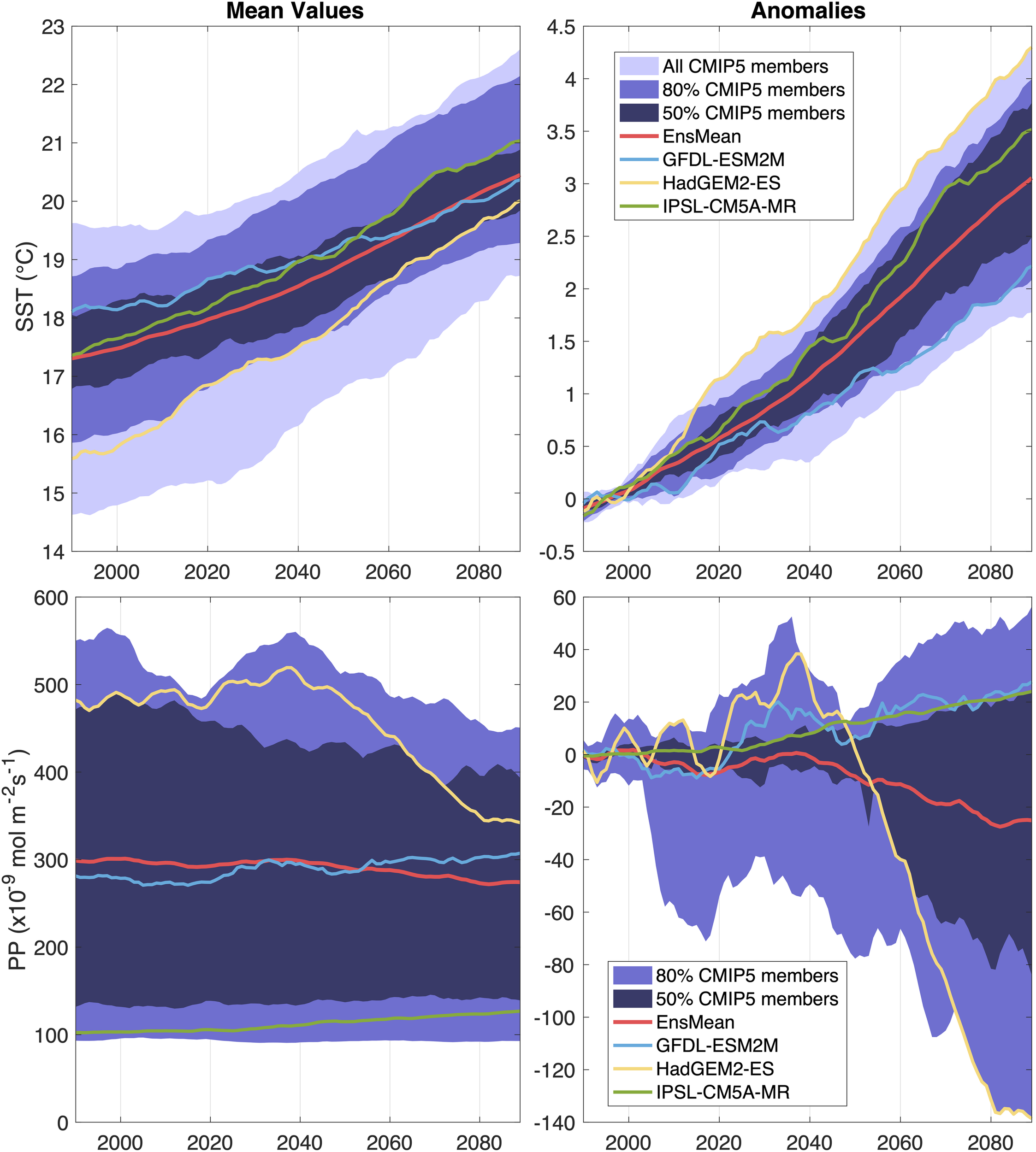
Time series of yearly averages of the California Current sea surface temperature (SST, first row) and primary production (PP, second row) for the 1976–2099 period, averaged over the California Current Large Marine Ecosystem. The simulations are forced using historical emissions (1976 to 2005) and the RCP8.5 scenario for future projection (2006 to 2099). Left panels show the mean values and right panels show the anomalies relative to the 1976–2005 climatology. A 20-year running mean is applied. The figure is adapted from the NOAA climate website (https://www.psl.noaa.gov/ipcc).
Downscaling Approach
Output from the selected ESMs provide the surface and ocean boundary conditions for ROMS-NEMUCSC in a one-way downscaling approach. To reduce biases exhibited in the ESMs historical simulations, we apply a “time-varying delta” bias-correction method prior to downscaling the ESMs output. We first estimate time-varying deltas (DELTA) for a forcing atmospheric variable (ATM) by subtracting the ESM’s historical monthly climatology (ESMCLM; years 1980–2010) from the whole period of interest (i.e., 1980–2100).
These monthly time-varying deltas are first bilinearly interpolated in space and time to the resolution of the reanalysis data used to force the control run (REAN), and then added to the monthly reanalysis climatology (REANCLM). Finally, we add high-frequency variability from the reanalysis (REANHF), computed as the residual after removing a 30-day running mean, as the absence of this high-frequency variability and associated damping of upwelling can lead to a biased ecosystem state (Gruber et al., 2006, 2011). The climatology and high-frequency component from the reanalysis (i.e., REANCLM and REANHF) are repeated (∼4 times) to cover the whole period of interest. Thus, for each ATM, the bias-corrected forcing ATM′ is computed as:
Bias correction for the ocean and biogeochemical variables is handled similarly, but with several adjustments for the lower frequency of available ESM output. The high-frequency component (REANHF) is excluded, since the available ESM output for 3D physical and biogeochemical variables have monthly and annual temporal resolution, respectively. In addition, the time-varying deltas for the biogeochemical variables are calculated annually, again because the ESM biogeochemical outputs are available at annual resolution (Table 1). Model initialization is handled similarly to the ocean boundaries by applying deltas from the year 1980 to our CTRL initial conditions.
The time-varying delta method for downscaling retains the observed historical climatology and high-frequency (sub-monthly) variability while inheriting the long-term change and interannual variability of the parent ESM. Relative to a “fixed delta” method that compares a historical period to a future one (e.g., Alexander et al., 2019; Shin and Alexander, 2020), the time-varying delta method has advantages of capturing projected changes in interannual variability, and resolving the full climate change evolution, including potentially non-linear impacts that would be missed when the transient response is excluded. An alternative method for prescribing the high-frequency variability would be to use the daily ESM forcing, which may be modulated by low-frequency variability (e.g., El Niño Southern Oscillation events alter storm tracks in the CCS). We retain the observed historical high-frequency variability from the reanalysis for several reasons. First, it allows us to force the model with high-resolution temporal forcing (6-hourly for the winds and hourly for the rest of ATMs), which resolves the daily cycle and is consistent with the historical forcing. Second, high frequency variability is likely to differ substantially within the space of a single ESM grid cell, particularly near the coast, and will not be resolved by the ESMs. In other EBUS, previous works applied statistical downscaling methods in the wind forcing to overcome the limitation of the coarse resolution models (e.g.,Goubanova et al., 2011; Machu et al., 2015; Bonino et al., 2019). While future changes in high frequency atmospheric forcing is not the focus of this study, it should be a topic of further research.
We refer to the downscaled simulations from ROMS-NEMUCSC, driven by GFDL, IPSL, and HAD as ROMS-GFDL, ROMS-IPSL, and ROMS-HAD, respectively, in the following sections and figures.
Observation Data for Model Evaluation
To evaluate the CTRL and the historical period of the downscaled simulations (i.e., ROMS-GFDL, ROMS-IPSL, and ROMS-HAD), we use the Optimum Interpolation SST data set, which combines in situ and satellite-based observations, from the National Oceanic and Atmospheric Administration (NOAA OISST v2; Reynolds et al., 2007) at 0.25° from 1982 to 2010 and for surface chlorophyll (chl), we use data from the Sea-viewing Wide Field-of-view Sensor (SeaWiFS) obtained from the National Aeronautics and Space Administration (NASA) Ocean Color Website (NASA Goddard Space Flight Center, Ocean Ecology Laboratory, Ocean Biology Processing Group; 2014) at ∼0.1° resolution from 2000 to 2010. In addition, we evaluate simulated physical and biogeochemical fields with climatological data from the WOA derived from the World Ocean Database (oxygen, Garcia et al., 2013a; nitrate, Garcia et al., 2013b; temperature,Locarnini et al., 2013).
Results
In the following sections, we describe projected changes in the future physical and biogeochemical states of the CCS, first for the long-term mean changes for the 2070–2100 period with respect to the historical period (1980–2010) (i.e., Future – Historical) and then the time-dependent changes for the full transient runs (1980–2100).
Model Evaluation
The historical CTRL reproduces many aspects of the CCS physical and biogeochemical variability (Supplementary Figures 3, 4). The simulated annual mean SST has a weak warm bias over most of the domain and a weak cold bias along the northern boundary. The Southern California Bight (SCB) shows the largest SST bias (∼1.4°C), which is comparable with other numerical simulations of the CCS (e.g., Veneziani et al., 2009; Renault et al., 2016) and is likely due to the poor representation of cloud cover and the cross-shore gradient in alongshore winds resulting from coarse spatial resolution in the forcing reanalysis data (Renault et al., 2020). The annual mean subsurface patterns of nitrate and dissolved oxygen in the CTRL simulation are also well represented compared to climatological values from the WOA. Although the observed and simulated values of nitrate and oxygen differ near the coast, which cannot be resolved by the coarse horizontal resolution of the WOA grid (1° × 1°), the model reasonably reproduces the offshore spatial gradient and variability of climatological subsurface nitrate and dissolved oxygen (Supplementary Figures 3, 4). The observed and simulated annual mean chlorophyll exhibits similar onshore-offshore gradients. However, the main differences are located in the nearshore regions, where the model overestimates chlorophyll between the northern San Francisco Bay (SFB) and Cape Blanco, and underestimates it in the northern coastal domain (>44°N), SFB, and the SCB (Supplementary Figure 3).
Long-Term Mean Changes
Alongshore Wind Stress and Vertical Velocity
We use meridional wind stress as a proxy for the alongshore or upwelling favorable winds. In general, the three ESM-driven ROMS simulations exhibit an overall intensification (i.e., more negative) and a northern displacement (>39°N) of the meridional wind stress (Figure 2), consistent with prior analysis (Rykaczewski et al., 2015; Xiu et al., 2018). These equatorward wind stress anomalies oppose the mean wind stress (poleward) at the northern latitudes. However, there are some notable inter-model differences in the spatial variability. ROMS-GFDL and ROMS-IPSL show a strong increase centered in the northern nearshore regions (<200 km from the coast) of the CCS, while ROMS-HAD shows the center of this intensification offshore and in the northwest corner of the domain. While ROMS-GFDL exhibits the strongest intensification across the CCS domain, ROMS-IPSL exhibits a weaker intensification that is confined along the coastal domain, and ROMS-HAD shows this intensification confined to the northern part of the CCS. A strong decrease in alongshore wind stress over the southern part of the domain is projected in both ROMS-IPSL and ROMS-HAD, offshore in the former and nearshore in the latter.
FIGURE 2
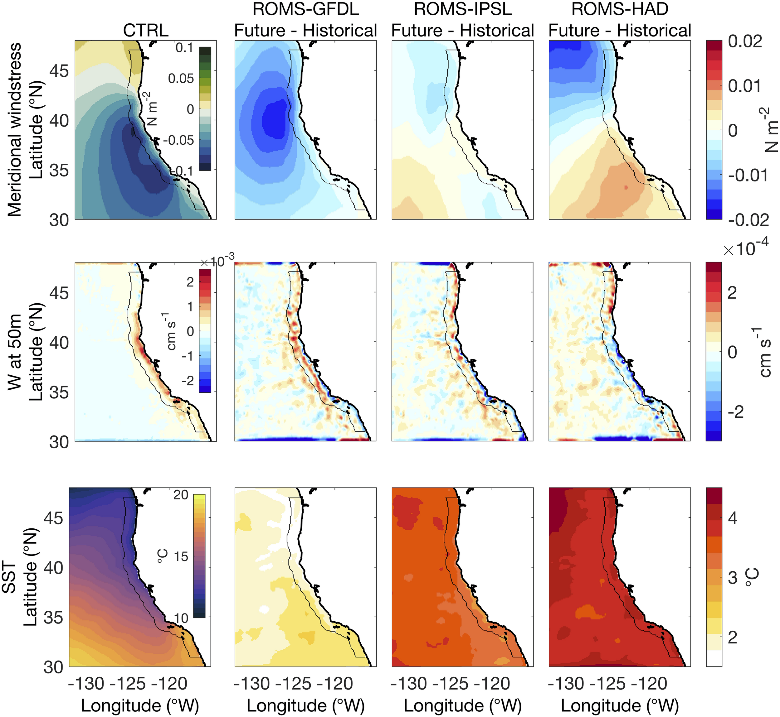
Control run (1980–2010) mean and future changes (2070–2100 relative to historical) for the physical variables. Rows show from top to bottom: meridional wind stress, vertical velocity at 50 m depth (w), and sea surface temperature (SST). Columns show data for the historical period in the control simulation (CTRL, first column) and the future changes from the high-resolution downscaled projections: ROMS-GFDL (second column), ROMS-IPSL (third column), and ROMS-HAD (fourth column). Negative values of wind stress changes correspond to an increase in equatorward wind stress. Black contour marks 100 km from shore. Vertical velocity field has been spatially smoothed out for better representation.
We use vertical velocity at 50 m as a measure for upwelling (Figure 2). The projected increase in the equatorward meridional wind stress over the northern coastal region of the CCS enhances coastal upwelling (upward and positive vertical velocity changes) in the three ESM-driven downscaled ROMS simulations. While ROMS-GFDL and ROMS-IPSL projections show an overall upward velocity all along the coast of the domain, the intense weakening of the alongshore-wind stress projected by ROMS-HAD reduces coastal upwelling in the southern part of the domain.
Sea Surface Temperature
The SST response to projected climate change includes warming over the entire domain in all three ESM-driven ROMS simulations (Figure 2). Although the three ROMS simulations agree on the warming of the CCS region, the magnitude of change differs considerably among simulations. ROMS-GFDL exhibits the weakest projected warming (<2.5°C), ROMS-IPSL a moderate warming (>3°C), and the ROMS-HAD the strongest warming (>3.5°C). In addition to the differences in overall climate sensitivity, there are differences among the spatial warming patterns: in the ROMS-IPSL the warming offshore of the SCB is relatively smaller, while ROMS-HAD presents a more homogeneous warming pattern. In ROMS-IPSL, this weaker warming extends north along the coast up to ∼43°N. In ROMS-GFDL, the warming is lessened in the northern coastal waters (>39°N), suggesting that increased wind-driven upwelling may partially mitigate the warming locally, while the strongest warming occurs in the offshore waters of the SCB.
Subsurface Nitrate
The ecological effects of upwelling critically depend on the biogeochemical properties and composition of upwelled source waters. To explore the subsurface biogeochemical properties, we select a depth of 150 m (Chhak and Di Lorenzo, 2007), which is deeper than the seasonal historical mixed layer depth (MLD) which ranges from 30 to 100 m in the whole domain. All three downscaled simulations project an increase of the subsurface nitrate concentration in the offshore waters (>100 km from the coast), with a larger increase by the end of the 21st century in ROMS-GFDL (∼5 mmol/m3) than in the other two simulations (∼2.5–3 mmol/m3) (Figure 3). However, the projections differ in the coastal waters (<100 km from the coast). While ROMS-GFDL shows a coastwide nitrate increase, the nitrate increase in ROMS-IPSL is much weaker and limited to the southern and northern CCS, and ROMS-HAD projects a decrease in subsurface nitrate along the coast, which is strongest in the southern part of the domain (Figure 3).
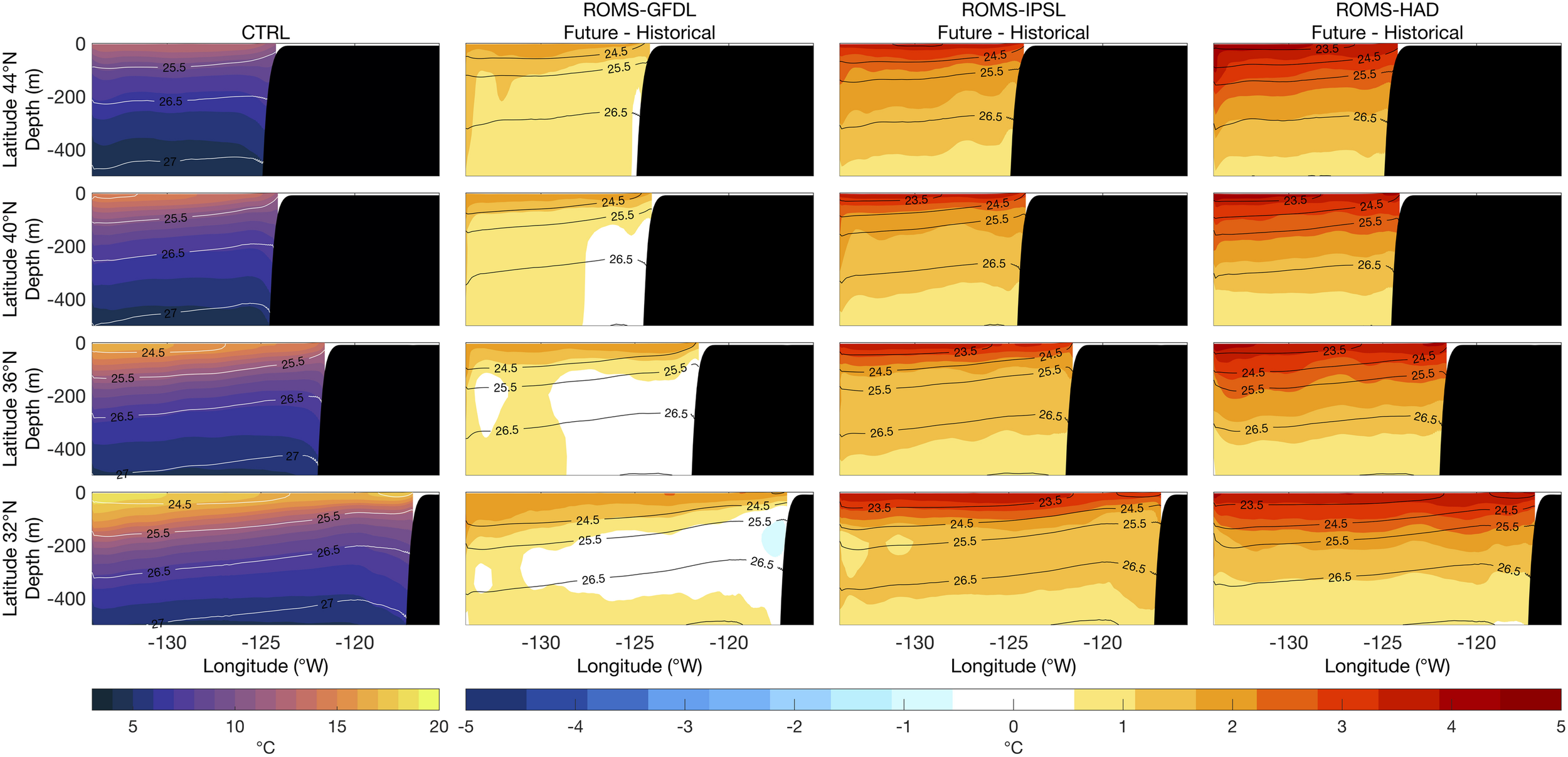
FIGURE 3
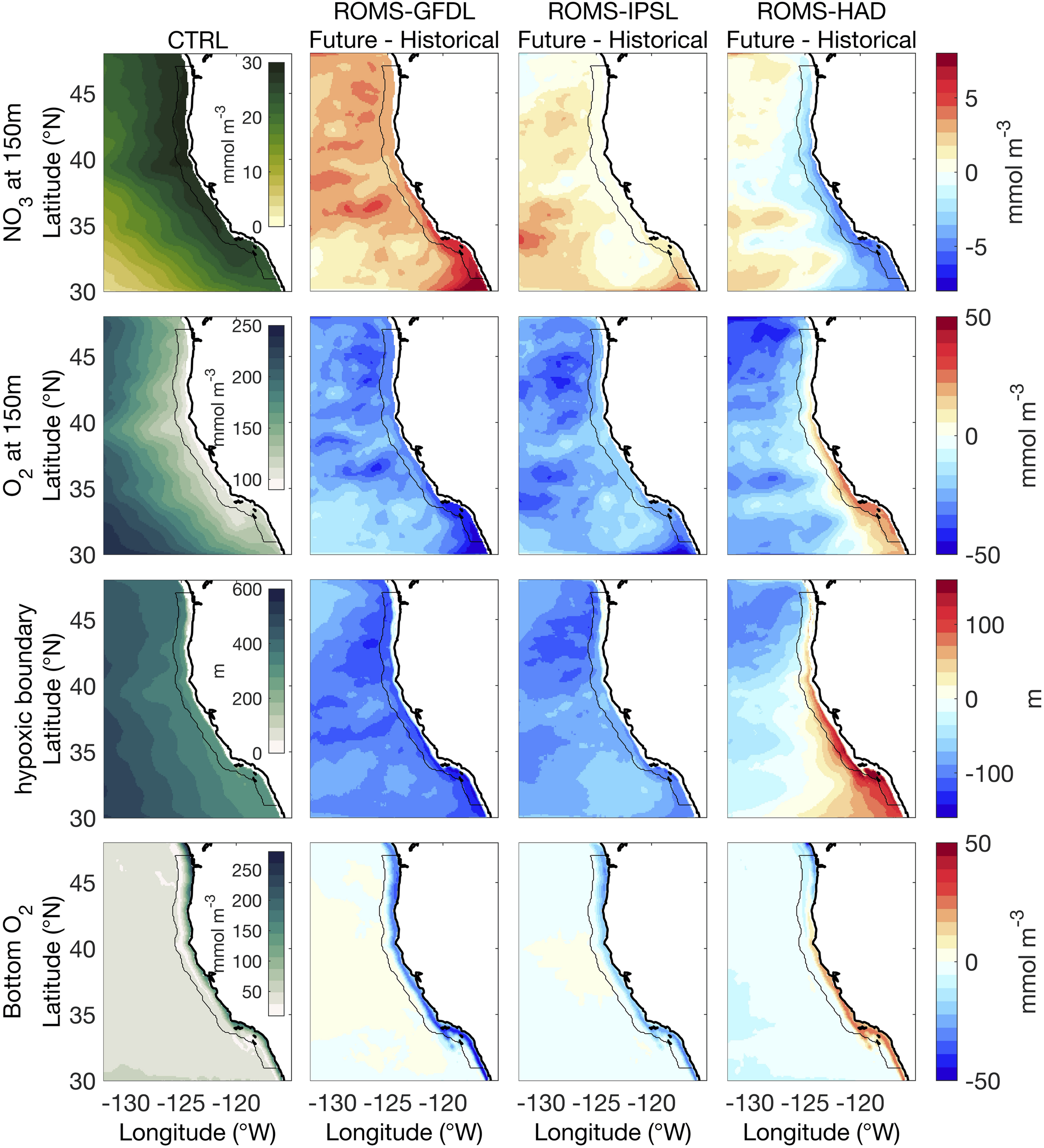
Control run (1980–2010) mean and future changes (2070–2100 relative to historical) for the subsurface biogeochemical variables. Rows show from top to bottom: nitrate (NO3) and dissolved oxygen at 150 m depth (O2), depth of 1.43 ml/l (i.e., 63.86 mmol/m3) O2 layer, and bottom oxygen. Columns show data for the historical period in the control simulation (CTRL, first) and the future changes from the high-resolution downscaled projections: ROMS-GFDL (second column), ROMS-IPSL (third column), and ROMS-HAD (fourth column). Black contour marks 100 km from shore.
Subsurface Oxygen
Below the seasonal pycnocline, upwelling systems are characterized by both high nutrient concentrations and low oxygen concentrations. The projected dissolved oxygen changes at 150 m depth mirror the nitrate changes described above – all three models exhibit large-scale oxygen declines. ROMS-HAD diverges from the others with a weak increase in dissolved oxygen that extends in the coastal waters from the southern boundary up to ∼40°N (Figure 3). Other ecologically important measures of the oxygen environment – bottom oxygen concentration and depth of the hypoxic boundary – show similar changes. While ROMS-GFDL and ROMS-IPSL projections feature a decline of bottom dissolved oxygen on the shelf, which is more intense (∼50 mmol m3) in the northern and southern coastal waters, ROMS-HAD projects a weak increase (∼25 mmol m3) of the bottom dissolved oxygen that extends from the southern coastal waters up to 40°N (Figure 3). Future changes in depth of the hypoxic boundary layer have a similar spatial pattern as the O2 at 150 m. The hypoxic boundary, defined here as the depth at which dissolved oxygen = 1.43 ml/l (i.e., 63.86 mmol/m3), is projected to shoal by up to ∼150 m in the offshore waters. Along the coast there is a weak shoaling, up to ∼60–70 m, in ROMS-GFDL and ROMS-IPSL, while ROMS-HAD projects changes of similar magnitude but opposite sign off southern and central California (Figure 3).
Phytoplankton Biomass
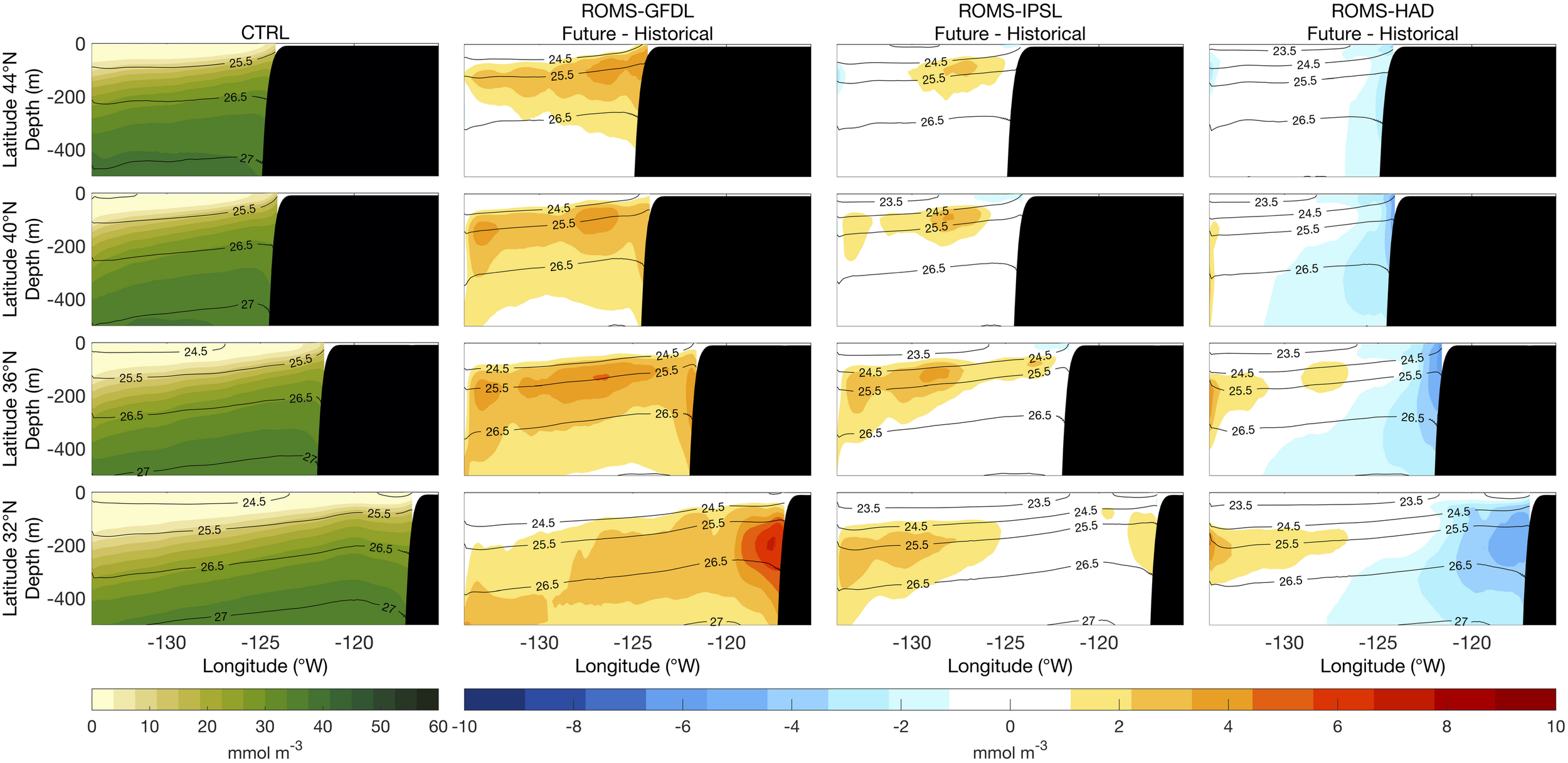
We present total phytoplankton biomass – the sum of NEMUCSC’s small (nanophytoplankton) and large (diatoms) phytoplankton groups – in units of chlorophyll concentration, which is estimated from NEMUCSC’s nitrogen units using fixed ratios for C:N (106:16) and C:Chl (50:1 and 100:1 for small and large phytoplankton, respectively, Goebel et al., 2010). By the end of the century, ROMS-HAD projects a decrease of surface chlorophyll along the entire coast; ROMS-IPSL projects a weaker decrease along most of the coast but a slight increase in the northern regions; and in contrast, ROMS-GFDL projects an increase centered in in the northern CCS (>39°–45°N), coincident with the region of most pronounced increases in upwelling favorable winds (Figure 4). Offshore, ROMS-IPSL and ROMS-HAD project a decrease in surface chlorophyll everywhere, while in ROMS-GFDL surface chlorophyll change is mostly positive north of 35°N. For ROMS-GFDL and ROMS-HAD, projected changes in vertically integrated chlorophyll over the upper 50 m exhibit similar patterns to surface chlorophyll changes. However, for ROMS-IPSL the slight increase in surface chlorophyll in the nearshore northern CCS is offset by subsurface chlorophyll decrease such that the upper 50 m integrated chlorophyll is projected to decline (Figure 4). In sum, phytoplankton biomass is projected to decline throughout the study domain with the exception of the northern CCS, where enhanced biomass is projected in ROMS-GFDL and ROMS-IPSL, though only for a shallow nearshore layer in the latter.
FIGURE 4
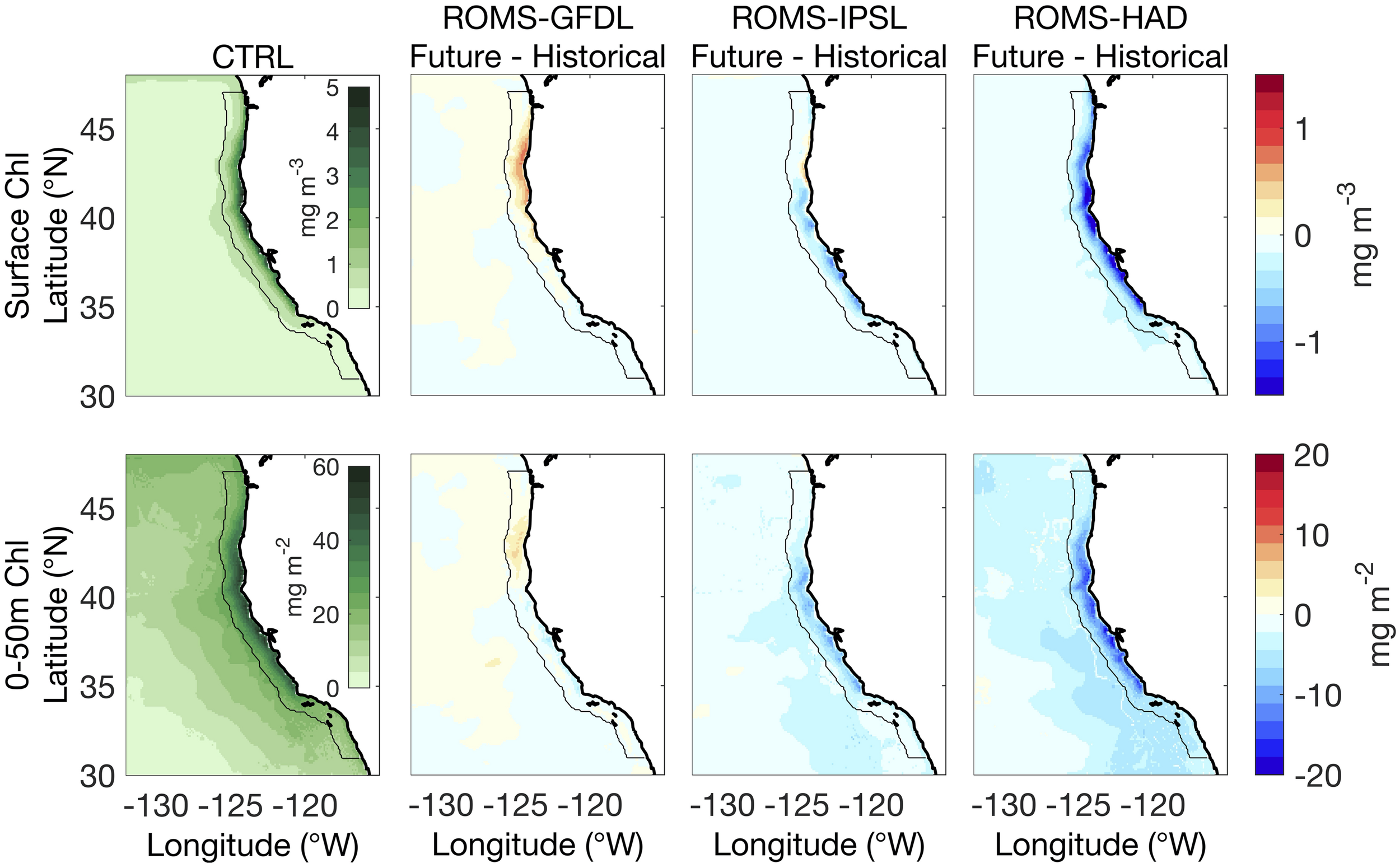
Control run (1980–2010) mean and future changes (2070–2100 relative to historical) for the surface (top) and integrated (0–50 m, bottom) chlorophyll (Chl). Columns show data for the historical period in the control simulation (CTRL, first) and the future changes from the high-resolution downscaled projections: ROMS-GFDL (second column), ROMS-IPSL (third column), and ROMS-HAD (fourth column). Black contour marks 100 km from shore.
Vertical Sections
All three downscaled simulations show an overall increase in temperature in the subsurface, with the warming being surface-intensified such that there is also an increase in stratification (i.e., more tightly packed potential density contours or isopycnals) by the end of the century (Figure 5). ROMS-HAD and ROMS-IPSL project warming changes up to ∼2°C at 300 m depth, and warming of ∼1°C extends to 500 m or more. As for SST, ROMS-GFDL indicates less subsurface warming than the other two projections, with weak warming in the northern latitudes, almost no change in the southern latitudes, and even a slight cooling of ∼0.5°C around ∼150 m depth in the nearshore southern CCS (32°N; Figure 5).
FIGURE 5
Vertical sections of mean temperature (1980–2010) from the control run (CTRL, first column) and of future temperature changes (2070–2100 relative to historical) from the high-resolution downscaled projections: ROMS-GFDL (second column), ROMS-IPSL (third column), and ROMS-HAD (fourth column). Black contours are potential density (kg m–3) relative to sea surface.
The inter-model consistency of the projected nitrate changes is spatially dependent. All three projections show subsurface increases in nitrate concentration offshore, though ROMS-GFDL shows a stronger increase with greater horizontal and vertical extent compared to the other models (Figure 6). However, the changes diverge near the coast. At 32°N and ∼200 m depth, in the core of the California Undercurrent (CU; i.e., ∼26.5 kg m–3), there is an increase of nitrate concentration in ROMS-GFDL but a decrease in ROMS-HAD. In both models, the inshore change in concentration extends north of 32°N, but with reduced magnitude (Figure 6). In contrast, ROMS-IPSL exhibits no discernible change in nearshore nitrate concentrations.
FIGURE 6
Vertical sections of mean nitrate (1980–2010) from the control run (CTRL, first column) and of future nitrate changes (2070–2100 relative to historical) from the high-resolution downscaled projections: ROMS-GFDL (second column), ROMS-IPSL (third column), and ROMS-HAD (fourth column). Black contours are potential density (kg m–3) relative to sea surface.
The future changes of spatial patterns of dissolved oxygen generally follow those of nitrate concentration with opposite signs (Figure 7), though the oxygen declines are more pronounced and widespread than the nitrate increases. There is a strong decrease in dissolved oxygen nearly everywhere in all of the projections, with the most pronounced decreases occurring slightly deeper in the south than in the north. Accompanying the nitrate concentration changes around the core of the CU, ROMS-GFDL and ROMS-IPSL project a decrease in oxygen, which is again stronger in ROMS-GFDL, while ROMS-HAD projects an increase of oxygen in the CU core at 32°N that vanishes quickly to the north. The association of enhanced nitrate and decreased oxygen is consistent with “older” subsurface waters adjacent to the California Current upwelling (e.g., Rykaczewski and Dunne, 2010; waters adjacent to the California Current upwelling have been isolated from the ocean surface for a longer period, allowing more nitrate to accumulate and more oxygen to be lost through aerobic remineralization of sinking organic material).
FIGURE 7
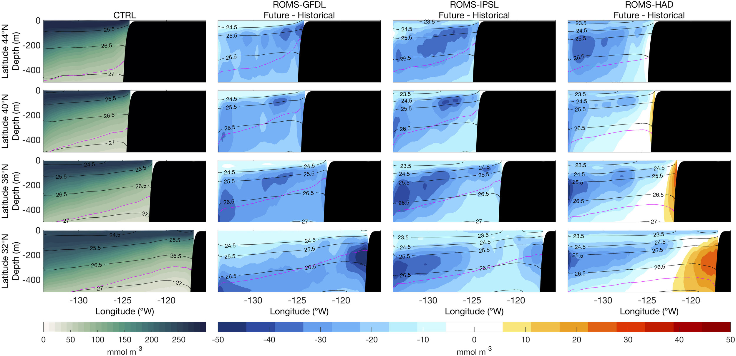
Vertical sections of mean dissolved oxygen (1980–2010) from the control run (CTRL, first column) and of future nitrate changes (2070–2100 relative to historical) from the high-resolution downscaled projections: ROMS-GFDL (second column), ROMS-IPSL (third column), and ROMS-HAD (fourth column). Black contours are potential density (kg m–3) relative to sea surface. Magenta contour corresponds to the hypoxic boundary layer (1.43 ml/l or 63.86 mmol/m3 O2).
FIGURE 8
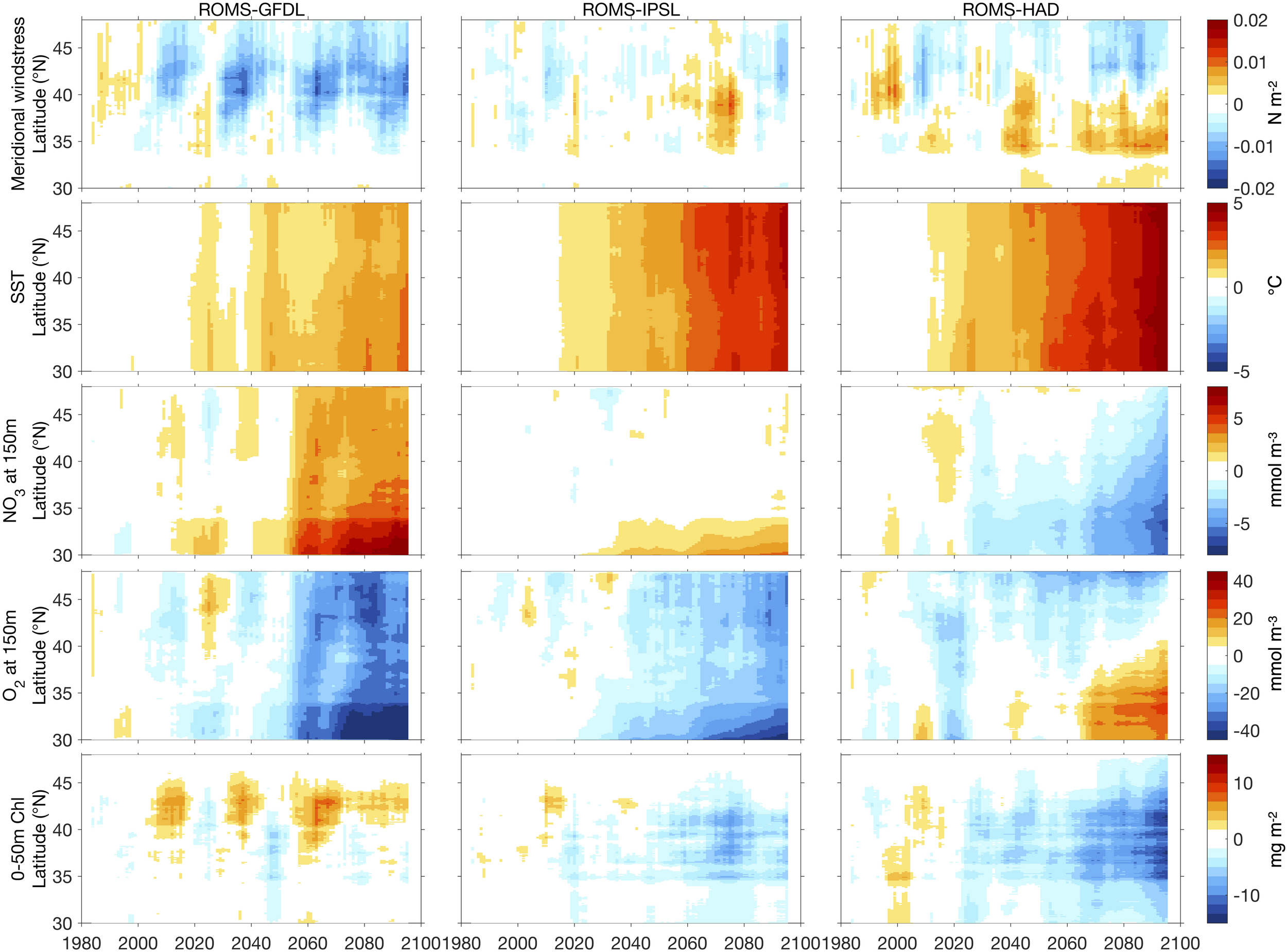
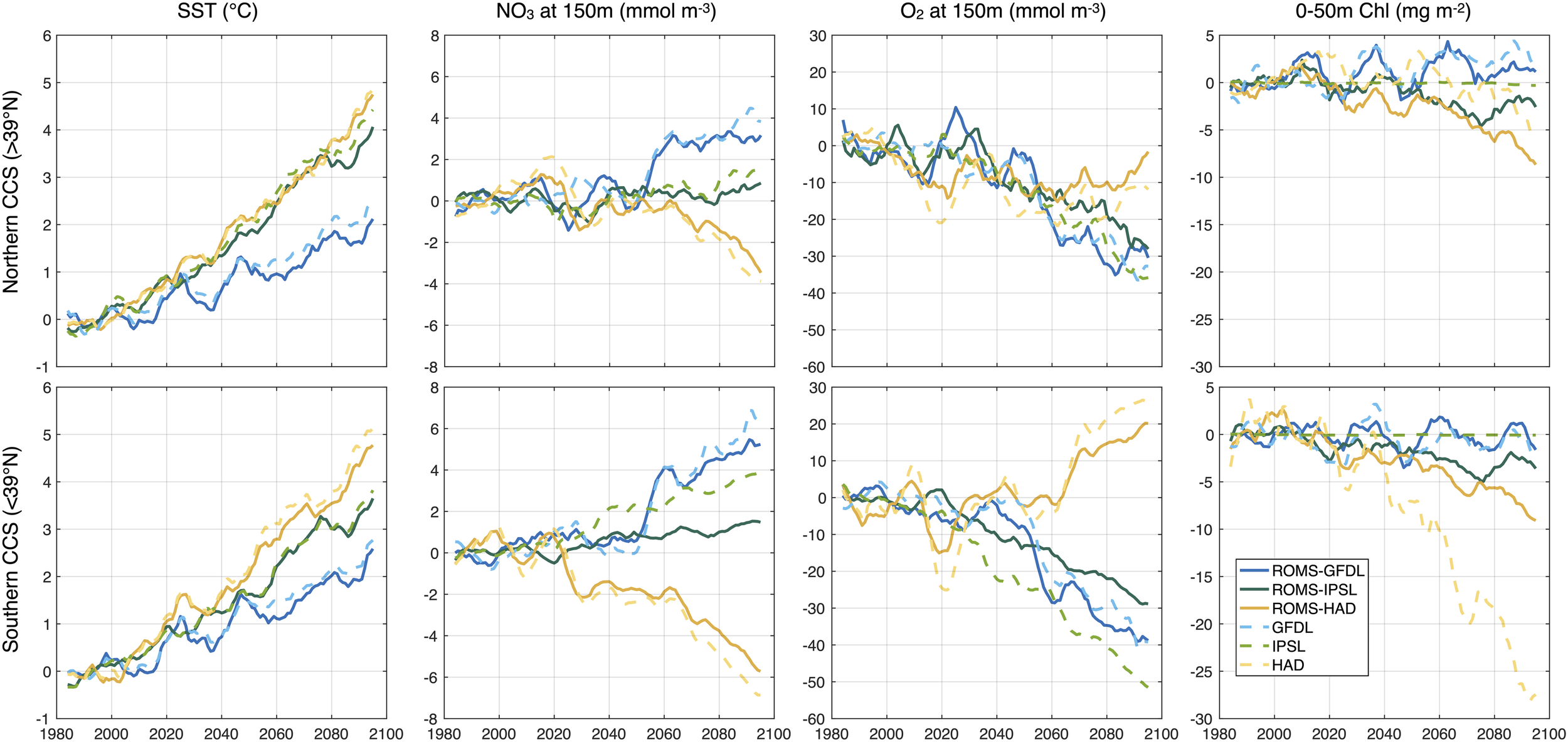
Hovmöller diagrams of 10-year running mean annual anomalies averaged from the coast to 100 km offshore of meridional wind stress (top row), SST (second row), nitrate (third row) and dissolved oxygen (fourth row) at 150 and 0–50 m integrated chlorophyll (bottom row) with respect to the historical period (1980–2010), from the high-resolution downscaled projections: ROMS-GFDL (left), ROMS-IPSL (center), and ROMS-HAD (right).
Coastal Trends and Long-Term Variability
Alongshore Wind Stress
Projections of wind stress across the three simulations share a common meridional pattern with intensification of equatorward (upwelling-favorable) wind stress in the northern CCS and unchanged or slightly weakened winds in the southern and central CCS (Figure 8). This pattern is consistent with previous analysis of CMIP5 models (Rykaczewski et al., 2015), but there are noticeable differences between simulations in the magnitude and timing of change throughout the 21st century. In ROMS-GFDL, the strongest intensification in upwelling favorable winds, centered between 40 and 45°N, becomes apparent by 2030 and persists through the end of the century. ROMS-IPSL shows low frequency variability without strong linear trends; in particular there is a period of considerably weakened upwelling favorable winds north of 35°N from approximately 2060–2080 followed by an intensification from 2080 through the end of the century. The prominence of these signals throughout the projections suggests the influence of decadal variability in this system, which can delay the emergence of anthropogenic upwelling trends until the late 21st century (Brady et al., 2017). ROMS-HAD has a consistent trend of equatorward wind stress intensification in northern latitudes and weakening in southern latitudes, with the division between increasing and decreasing upwelling favorable winds at ∼40°N.
Sea Surface Temperature
Surface ocean warming is one of the most robust ocean responses to climate change, and all three simulations project increases in SST across all latitudes (Figure 8). SST continues to increase with time in all simulations, with ROMS-GFDL projecting the weakest increase (∼2.5°C by 2090), ROMS-IPSL projecting a stronger increase (∼4°C by 2090), and ROMS-HAD projecting the strongest increase (∼5°C by 2090). ROMS-GFDL projects slightly stronger warming at southern latitudes, while ROMS-IPSL and ROMS-HAD project nearly uniform warming across the meridional extent of the coastal domain.
Subsurface Nitrate Concentration
Regional Ocean Modeling System-Geophysical Fluid Dynamics Laboratory projects a strong increase in subsurface nitrate concentration, with a trend that emerges from the natural variability (i.e., exceeds 1 standard deviation of the historical variability) by ∼2050 and is strongest from 30° to 35°N (Figure 8). ROMS-IPSL exhibits a similar spatial pattern, but with a reduced trend that exceeds decadal variability only in the southern part of the domain and that is inherited from the parent ESM. The nearshore decrease in nitrate concentration in ROMS-HAD emerges clearly in roughly 2060 in the southern latitudes and spreads northward across most of the domain by the end of the century (Figure 8).
Subsurface Dissolved Oxygen
Projected dissolved oxygen concentrations generally follow those of the nitrate concentrations, with opposite signs, across all three models (Figure 8). The tight coupling between nitrate and oxygen is evident both in the decadal variability and in the long-term trends, though the oxygen trends are even more pronounced. While all three models project a strong decrease in dissolved oxygen, particularly in the northern latitudes, the time when the dissolved oxygen changes becomes prominent differs among models. Trends emerge from the natural variability across all latitudes by ∼2060 and ∼2040 in ROMS-GFDL and ROMS-IPSL, respectively. In ROMS-HAD, an oxygen decrease has already emerged in the northern latitudes (>43°N), while decadal variability remains the dominant signal in the rest of the domain, and beyond 2070, a weak increase in dissolved oxygen emerges in the southern part of the domain, consistent with the decrease of nitrate there.
Vertically Integrated Phytoplankton Biomass
All three models project the main changes in chlorophyll, vertically integrated over 0–50 m, along a latitude band between 35 and 45°N, the most productive portion of the CCS (Figure 8). ROMS-HAD and ROMS-IPSL project a chlorophyll decrease starting in ∼2040 and ∼2050, respectively, near 37°N, which strengthens and extends across most of the coastal domain by the end of the century in ROMS-HAD. In contrast, ROMS-GFDL projects an increase of vertically integrated chlorophyll (∼8 mg m2 that becomes distinct ∼2050), off Northern California and Oregon (∼40–45°N) and a decrease off Central California (∼35–37°N). These changes in ROMS-GFDL are likely driven by both the intensification of the alongshore winds, which increase the upwelling between 40° and 45°N, and the strong increase of the subsurface nitrate concentration. In ROMS-HAD, the negative trends in vertically integrated chlorophyll are largely consistent with trends in the weakening of the upwelling-favorable wind stress and the decrease of subsurface nitrate concentration along the southern (<39°N) CCS coast. However, along the northern (>39°N) CCS coast, these negative trends in chlorophyll indicate that the intensification of alongshore winds cannot offset the depletion of subsurface nitrate. However, the dynamics driving chlorophyll changes are not necessarily straightforward, as phytoplankton biomass can be influenced by changes in upwelling strength, subsurface nutrients, upper ocean stratification, and top-down control by grazers. The relative influence of these potentially competing drivers under historic and future forcing continues to be a topic of interest, which we discuss more in the following section.
Coastal Trends ESMs Comparisons
To highlight the impact of the downscaling process, we compare coastal trends of key ecosystem variables with those of the ESMs (Figure 9). All projections show a strong warming of the coastal CCS. SST increases rapidly in the ROMS-IPSL and in ROMS-HAD from the late 2020s, and late 2030s. By the end of the century, SST increases in ROMS-IPSL reach ∼4°C and >3.5°C in the northern and southern CCS, respectively, while in ROMS-HAD warming reaches >4.5°C in both the northern and southern regions. ROMS-GFDL shows a moderate increase in SST, starting later (∼2040), and reaching ∼2°C and >2.5°C, in the northern and southern CCS, respectively, by the end of the century. SST trends in the downscaled projections strongly followed those from the ESMs, resulting in no significant spread between the downscaled projections and their ESMs counterparts. Compared to the evolution of the ROMS-ESM SST means, the SST ESMs exhibit an offset of the trends due to their different bias with respect to the historical period (∼1–2°C, Supplementary Figure 5).
FIGURE 9
From left to right time series of yearly averaged anomalies with respect to the historical period averaged from the coast to 100 km offshore of SST, NO3 and O2 at 150 and 0–50 m vertically integrated chlorophyll for the northern (top, >39°N) and southern (bottom, <39°N) CCS.
Biogeochemical variables in ROMS-ESMs show different signs in the trends along the CCS coast. These changes and their meridional differences in magnitude are consistent with those from ESMs (Figures 9, 10). In ROMS-GFDL and ROMS-HAD, the evolution of subsurface nitrate and oxygen agree more closely with their ESM counterparts. However, the evolution of these anomalies in ROMS-IPSL separate from those in the IPSL, showing a significant intra-model spread especially in the southern coastal region.
FIGURE 10
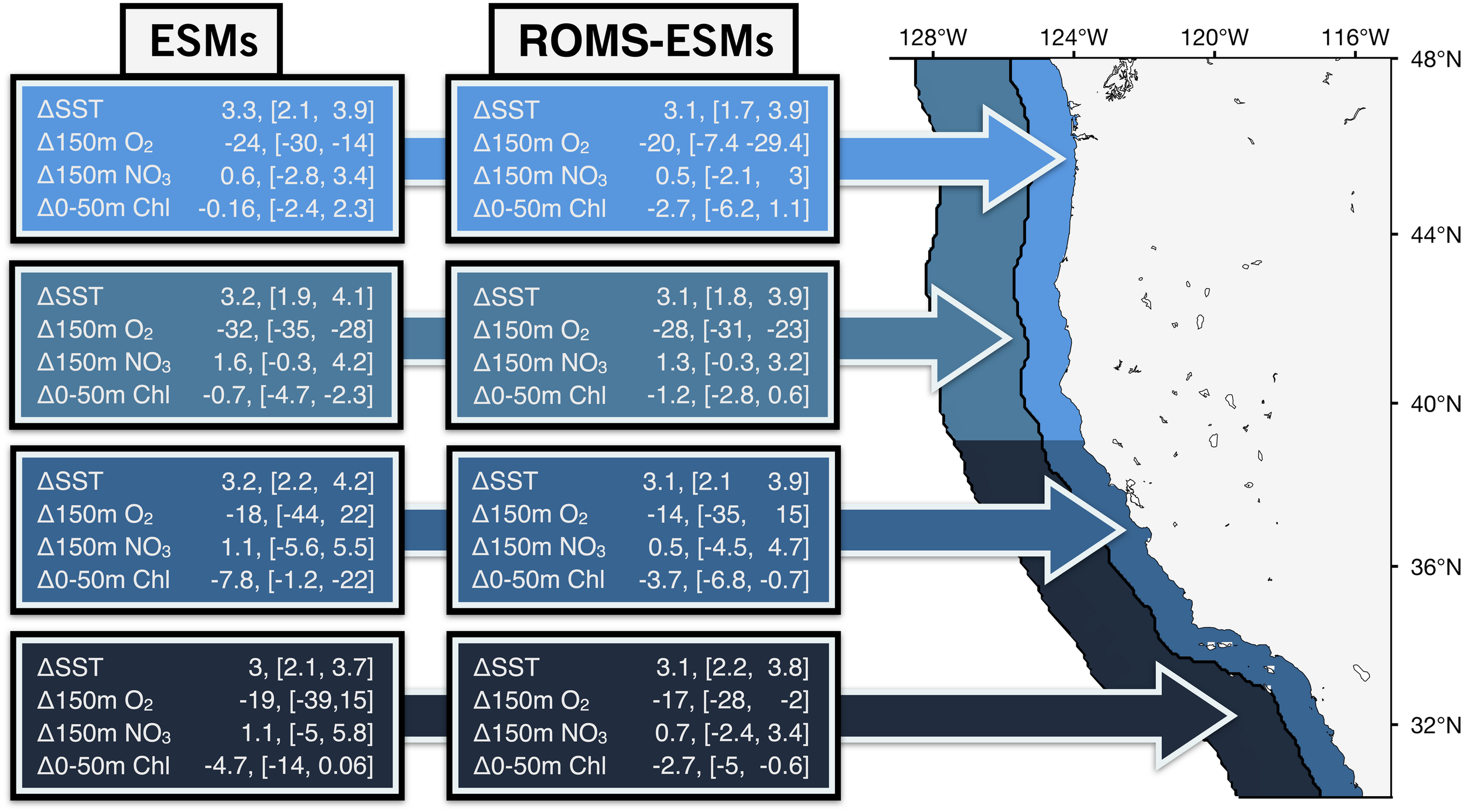
Schematic table summarizing the main physical and biogeochemical variables future changes for the period (2070–2100), from the ESMs (left) and ROMS-ESMs (right) projections for the nearshore (from a distance of 100 km to the coast) and offshore (from 100 to 300 km) for the northern and southern CCS coast. The variables listed are: SST (°C), NO3 and O2 at 150 (mmol/m3) and 0–50 m vertically integrated chlorophyll (mg/m2). For each variable, the mean change and inter-model range change during the period are shown.
Regional Ocean Modeling System-Institut Pierre Simon Laplace and ROMS-HAD depict a moderate and a strong decline of coastal chlorophyll along the coast, reaching −0.5 and −10 mg m–2 by the end of the century, respectively. Meanwhile, ROMS-GFDL depicts a moderate increase of chlorophyll in the northern CCS coast. The evolution of the ROMS-GFDL chlorophyll trends agrees more closely with those from GFDL, showing a pronounced decadal variability. However, ROMS-IPSL and ROMS-HAD show a larger spread in chlorophyll with respect to their counterparts. While anomalies of chlorophyll in IPSL remain unchanged during the century, the chlorophyll in ROMS-ISPL declines, showing larger variability than the chlorophyll projection in IPSL (Figure 9).
Because of the inherent ESM bias with respect to the historical period, the evolution of the mean values of the biogeochemical variables also exhibit an offset compared to those in the ROMS-ESMs. Offset magnitudes are larger in subsurface nitrate and oxygen in GFDL and IPSL, while chlorophyll offset is larger in HAD (Supplementary Figure 5).
Discussion
We used a coupled physical-biogeochemical model (ROMS-NEMUCSC) at 0.1-degree (∼10 km) resolution to produce downscaled projections of climate change in CCS from 1980 to 2100 under the high emissions RCP8.5 scenario. To capture the spread of projections, we selected three ESMs, GFDL-ESM2M, HadGEM2-ES, and IPSL-CM5A-MR, that span the CMIP5 range for future changes in both the mean and variance of physical and biogeochemical CCS properties. The downscaled runs provide information on potential future physical and biogeochemical states in the CCS at higher resolution than those available from current generation ESMs. More importantly, they provide insight into which future changes are robust (i.e., with different projections agreeing on the sign of change, if not the magnitude) and which are uncertain even in a qualitative sense (i.e., when models diverge on the sign of changes). They also illustrate benefits and limitations of dynamical downscaling in the context of climate change projection. We discuss these points below.
Similarities and Differences Among ESM-Driven ROMS Projections
All three downscaled models show an overall intensification of the meridional wind stress (i.e., equatorward wind stress or upwelling-favorable winds) in the northern part of the domain (>40°N), consistent with previous work (Rykaczewski et al., 2015; Wang et al., 2015; Xiu et al., 2018), with ROMS-IPSL showing the weakest intensification and ROMS-GFDL the strongest. In the southern region, ROMS-GFDL and ROMS-IPSL show a weaker intensification of the upwelling-favorable wind stress, while ROMS-HAD projects a weakening wind stress. Although, ROMS-GFDL and ROMS-IPSL simulations project an intensification of the upwelling-favorable wind stress for the last thirty years of the end of the century, ROMS-IPSL projects a weakening of the meridional wind stress in coastal waters from approximately 2060–2080. Since low frequency variability in the dynamically downscaled surface winds remains dependent on the overlying larger-scale wind, this period of winds stress relaxation along the CCS coast in ROMS-IPSL may reflect variability in the North Pacific represented by the ESM model parent IPSL. Further analysis demonstrates that decadal-scale variability in upwelling-favorable wind stress in all three models is correlated with basin-scale climate oscillations (i.e., the Pacific Decadal Oscillation, PDO; Mantua et al., 1997). For example, weakened upwelling-favorable wind stress in ROMS-IPSL during 2050–2080 occurs during a positive phase of the PDO (Supplementary Figures 6, 7, and Supplementary Table 1). Without careful assessment, an analysis of the projections from ROMS-IPSL for this particular and short period of time (i.e., 2060–2080) could lead to misattributing this signal to anthropogenic climate change instead of natural climate variability (e.g., Deser et al., 2012). Thus, it is important to consider the simulation’s full transient period, or longer time-scales projections, as recommended in the downscaling protocols by Drenkard et al. (in review). It also justifies our approach of using a time-varying delta method to generate the downscaled projections.
In the subsurface offshore, the three ESM-driven ROMS simulations project similar enrichment of nitrate and a decrease in dissolved oxygen as well as a shoaling of the hypoxic boundary layer, all of which follow their ESM counterparts. In the coastal regions, ROMS-GFDL and ROMS-IPSL biogeochemical responses are similar in sign and aligned to those off the coast, featuring an average of ∼30–40% increase/decrease of subsurface nitrate/dissolved oxygen, ∼25% reduction of bottom oxygen on the shelf, and a ∼50 m shallower hypoxic boundary layer. ROMS-HAD projects a different response featuring a decrease of subsurface nitrate (∼20%) that by 2070 extends along the entire coast, an increase of subsurface oxygen (30%) in the southern region that extends to the bottom of the shelf, and a deepening of the hypoxic boundary layer by ∼30 m. Changes in subsurface nitrate and oxygen in our ROMS projections are largely consistent with recent downscaling studies that include these ESMs (Xiu et al., 2018; Howard et al., 2020a). One exception is subsurface oxygen in ROMS-HAD along the coast, for which we find an increase in oxygen coupled to the decrease in subsurface nitrate. Howard et al. (2020a) find that subsurface oxygen decreases in their downscaled HAD projection, though that decrease is much weaker than in their GFDL and IPSL projections. A plausible explanation for this may be associated with the downscaling method and/or the specific ensemble member from HAD used to force the high-resolution projections.
Changes in nutrient concentrations and nutrient ratios have already been observed in upwelling source waters of the CCS (e.g., Bograd et al., 2015). ROMS-GFDL and ROMS-IPSL projected trends in nitrate enrichment and deoxygenation are consistent with previous studies that suggest that biogeochemical changes in upwelling source waters could be a first order effect in changes in the biogeochemistry of the CCS, with the decrease in ventilation of North Pacific interior waters, increase in stratification and the subsequent deepening of the isopycnals, being the proposed driving mechanisms (Rykaczewski and Dunne, 2010; Xiu et al., 2018; Dussin et al., 2019; Howard et al., 2020a). Moreover, deoxygenation of the upwelling source waters is the main driver of changes in hypoxia and expansion of hypoxic areas on the shelf (Dussin et al., 2019). Under the future RCP8.5 scenario, HAD and IPSL project relatively small changes of Equatorial Undercurrent (EUC) transport compared to GFDL, accompanied by a slight compression of the oxygen minimum zones (OMZ) in the former and expansion in the latter (Shigemitsu et al., 2017). These models’ biases (i.e., representation of the EUC) and discrepancies in the future projections of the complex equatorial dynamics and the OMZ (Cabré et al., 2015; Busecke et al., 2019) could explain the diverse trends in the downscaled projections. The strong decrease of subsurface oxygen near the southern boundary projected by ROMS-GFDL might be associated with the weakening of the EUC and transport of older waters (i.e., less oxygen and higher nutrient concentrations) into the CCS from the south. In contrast, the increase of subsurface oxygen in the projected ROMS-HAD might be related to the compression of the OMZ and the transport of younger waters to the CCS. Future changes in the equatorial dynamics and their connections to the CCS source waters will be explored in future work.
The projected enrichment of nutrients in subsurface waters, combined with increased upwelling caused by the intensification of the meridional wind stress, could be the driving mechanisms for increases in the phytoplankton biomass of ∼50% in ROMS-GFDL. Enrichment of nutrients near the depth of upwelled source waters may increase primary productivity in the CCS (Rykaczewski and Dunne, 2010), but our results suggest that the increase in productivity is reinforced by the intensification of upwelling favorable winds projected to occur in the northern coastal CCS in ROMS-GFDL. Conversely, nutrient-poor source waters combined with the weakening of upwelling winds (15–18%) likely drive the projected strong decrease of chlorophyll (∼50%) in the coastal CCS by ROMS-HAD. This differing response of ROMS-HAD could come from inheriting the large-scale biogeochemical changes in HAD that propagate through the CCS boundaries.
All the models show that future ocean warming in the CCS is surface intensified, indicating enhanced stratification (Figure 5 and Supplementary Figure 8). In the coastal domain, ROMS-GFDL and ROMS-IPSL project the larger stratification and reduced (i.e., shallower) MLD around ∼34–40°N (between Point Conception and Cape Mendocino), while ROMS-HAD projects a weaker stratification and less shoaling of the MLD in that region (Supplementary Figure 8). Increased stratification can potentially counteract the effect of intensifying winds and source water nutrient enrichment by limiting the nutrient flux to the mixed layer and decreasing PP (Di Lorenzo et al., 2005; García-Reyes et al., 2015; Jacox et al., 2015). Thus, enhanced stratification, in combination with weakened upwelling-favorable winds, could explain why phytoplankton biomass decreases are projected in the southern CCS by ROMS-GFDL and along most of the coast by ROMS-IPSL despite increasingly nutrient-rich subsurface waters. The uncertainty related to the interplay between the thermal stratification and intensification of upwelling winds should be explored further.
Impact of Regional Downscaling
Given the added effort, computational cost, and storage required associated with dynamical downscaling, it is worth considering the added benefit relative to the uncertainties in the parent model forcing. We compared the ROMS projections with those from their ESM counterparts and showed that both SST and chlorophyll trends are qualitatively consistent between ROMS simulations and their ESM parents (Figure 9). ROMS-ESM SST changes follow those of their ESM parents closely in magnitude, producing a similar range of the uncertainties. From the ESM parent models, GFDL and IPSL agree on the sign of the NPP and surface chlorophyll change (i.e., increasing through the century), while the CMIP5 ensemble mean projects declines in NPP in this region with the same sign trend as HadGEM2-ES, but with much smaller magnitude (Figure 1). Along the CCS coast, ROMS-GFDL and ROMS-HAD also agree on the trend sign and the latitudinal expressions of the chlorophyll changes compared to their ESM parents, but not in the magnitude in the latter. On the other hand, ROMS-IPSL projects a clear negative trend in chlorophyll while the trend in IPSL is weaker (Figure 9 and Supplementary Figure 9). Differences in the sign and magnitude of the trends might be related to non-linear interactions in the biogeochemistry as a response to the upwelling dynamics that are better resolved in the downscaled models. Compared to the SST changes, some ROMS-ESM biogeochemical changes largely differ in magnitude from their ESM parents, producing larger intra-model spread in particular between ROMS-HAD and HAD in chlorophyll, and ROMS-IPSL and IPSL in subsurface nitrate and oxygen. However, there is an overall reduction of the uncertainty of the biogeochemistry projections in the ROMS-ESMs, likely due to using the same biogeochemical model and parameterization for all three downscaled simulations. A summary of these main physical and biogeochemical changes in the CCS is shown in Figure 10.
The larger biogeochemical differences between ROMS simulations and their ESM parent models illustrate the impact of regional downscaling’s ability to resolve local processes impacting productivity (Echevin et al., 2020). Various factors may explain why biogeochemical variables are more sensitive to regional downscaling than physical variables: (1) high-spatial resolution for the circulation is needed to simulate upwelling dynamics and their ecosystem responses; (2) complex nonlinear interactions occur between the physical changes and ecosystem responses; and (3) the formulation of the biogeochemical component varies among ESMs and is different than NEMUCSC, which has been specifically calibrated for the CCS.
Concluding Remarks
The high-resolution downscaled projections presented here belong to a broader end-to-end modeling project (Future Seas2) that integrates climate, biogeochemical, ecosystem, and socioeconomic models to evaluate the impacts of climate change in the CCS and evaluate fisheries management strategies under projected future conditions. The regional ocean models provide the physical and biogeochemical foundation for higher trophic level models of various types, including individual based models and species distribution models (Smith et al., 2021), highlighting the utility of high-resolution projections for regional marine resource applications. However, given that differences between downscaled models and their ESM parents can be small relative to the differences between ESMs, any specific application should consider the value of dynamical downscaling in the context of other sources of uncertainty. Until large ensembles of eddy-resolving global or regional models are computationally feasible, we suggest that a fruitful approach is to combine coarser resolution large ensembles with dynamical downscaling of select runs informed by analyses like the one presented here to assess how representative basin-scale changes are translated to shelf-scale responses.
Statements
Data availability statement
The regional model output is available on request from the corresponding author. CMIP5 model output is available through a distributed data archive developed and operated by the Earth System Grid Federation data portal (ESGF, https://esgf-node.llnl.gov/search/cmip5/). ERA-5, the fifth generation of ECMWF atmospheric reanalyses of the global climate, is available from the Copernicus Climate Change Service Climate Data Store website (https://cds.climate.copernicus.eu/cdsapp#!/home). The Cross-Calibrated Multi-Platform (CCMP) wind vector analysis product version 1.1 is available from(http://www.remss.com/measurements/ccmp/). NOAA High Resolution SST data by the NOAA/OAR/ESRL PSL, Boulder, Colorado, USA is available from their website https://psl.noaa.gov/. Sea-viewing Wide Field-of-view Sensor (SeaWiFS) chlorophyll data from the NASA Goddard Space Flight Center, Ocean Ecology Laboratory, Ocean Biology Processing Group is available from their website https://oceancolor.gsfc.nasa.gov/data/seawifs/. Finally, World Ocean Atlas database series are derived from the Word Ocean Database, and are available from https://www.nodc.noaa.gov/OC5/indprod.html.
Author contributions
MPB and MGJ designed the research. MPB and MAA downscaled the ESM models. MPB conducted the physical variables projections, and analyzed the data. JF produced the biogeochemical variables projections. MPB, MGJ, JF, MAA, SJB, ENC, CAE, RRR, and CAS wrote the manuscript.
Funding
This work was supported by a grant from the National Atmospheric and Oceanic Administration (NOAA) CPO Coastal and Climate Applications (COCA) program and the NOAA Fisheries Office of Science and Technology (NA17OAR4310268).
Acknowledgments
Many thanks to Isaac Schroeder and Liz Drenkard for helpful comments on an earlier version of the manuscript.
Conflict of interest
The authors declare that the research was conducted in the absence of any commercial or financial relationships that could be construed as a potential conflict of interest.
Supplementary material
The Supplementary Material for this article can be found online at: https://www.frontiersin.org/articles/10.3389/fmars.2021.612874/full#supplementary-material
References
1
Alexander M. A. Shin S. -i. Scott J. D. Curchitser E. Stock C. (2019). The response of the northwest atlantic ocean to climate change.J. Climate33405–428. 10.1175/jcli-d-19-0117.1
2
Alin S. R. Feely R. A. Dickson A. G. Hernández-Ayón J. M. Juranek L. W. Ohman M. D. et al (2012). Robust empirical relationships for estimating the carbonate system in the southern California current system and application to CalCOFI hydrographic cruise data (2005–2011).J. Geophys. Res.117:C05033. 10.1029/2011jc007511
3
Arellano B. Rivas D. (2019). Coastal upwelling will intensify along the Baja California coast under climate change by mid-21st century: insights from a GCM-nested physical-NPZD coupled numerical ocean model.J. Mar. Syst.199:103207. 10.1016/j.jmarsys.2019.103207
4
Arora V. K. Boer G. J. Friedlingstein P. Eby M. Jones C. D. Christian J. R. et al (2013). Carbon–Concentration and carbon–climate feedbacks in CMIP5 earth system models.J. Climate265289–5314. 10.1175/jcli-d-12-00494.1
5
Arora V. K. Katavouta A. Williams R. G. Jones C. D. Brovkin V. Friedlingstein P. et al (2020). Carbon–concentration and carbon–climate feedbacks in CMIP6 models and their comparison to CMIP5 models.Biogeosciences174173–4222. 10.5194/bg-17-4173-2020
6
Atlas R. Hoffman R. N. Ardizzone J. Leidner S. M. Jusem J. C. Smith D. K. et al (2011). A cross-calibrated, multiplatform ocean surface wind velocity product for meteorological and oceanographic applications.Bull. Am. Meteorol. Soc.92157–174. 10.1175/2010bams2946.1
7
Auad G. Miller A. Di Lorenzo E. (2006). Long-term forecast of oceanic conditions off California and their biological implications.J. Geophys. Res.111:C09008. 10.1029/2005jc003219
8
Bakun A. (1990). Global climate change and intensification of coastal ocean upwelling.Science247198–201. 10.1126/science.247.4939.198
9
Bakun A. Black B. A. Bograd S. J. Garcia-Reyes M. Miller A. J. Rykaczewski R. R. et al (2015). Anticipated effects of climate change on coastal upwelling ecosystems.Curr. Climate Change Rep.185–93. 10.1007/s40641-015-0008-4
10
Bakun A. Field D. B. Redondo-Rodriguez A. Weeks S. J. (2010). Greenhouse gas, upwelling-favorable winds, and the future of coastal ocean upwelling ecosystems.Global Change Biol.161213–1228. 10.1111/j.1365-2486.2009.02094.x
11
Bograd S. J. Buil M. P. Lorenzo E. D. Castro C. G. Schroeder I. D. Goericke R. et al (2015). Changes in source waters to the Southern California Bight.Deep Sea Res. Part II Top. Stud. Oceanogr.11242–52. 10.1016/j.dsr2.2014.04.009
12
Bograd S. J. Schroeder I. D. Jacox M. G. (2019). A water mass history of the Southern California current system.Geophys. Res. Lett.466690–6698. 10.1029/2019gl082685
13
Bonino G. Di Lorenzo E. Masina S. Iovino D. (2019). Interannual to decadal variability within and across the major Eastern Boundary Upwelling Systems.Sci. Rep.9:19949. 10.1038/s41598-019-56514-8
14
Bopp L. Resplandy L. Orr J. C. Doney S. C. Dunne J. P. Gehlen M. et al (2013). Multiple stressors of ocean ecosystems in the 21st century: projections with CMIP5 models.Biogeosciences106225–6245. 10.5194/bg-10-6225-2013
15
Boville B. A. Gent P. R. (1998). The NCAR climate system model, version One∗.J. Climate111115–1130. 10.1175/1520-04421998011<1115:Tncsmv<2.0.Co;2
16
Brady R. X. Alexander M. A. Lovenduski N. S. Rykaczewski R. R. (2017). Emergent anthropogenic trends in California current upwelling.Geophys. Res. Lett.445044–5052. 10.1002/2017gl072945
17
Bruyère C. L. Done J. M. Holland G. J. Fredrick S. (2014). Bias corrections of global models for regional climate simulations of high-impact weather.Clim. Dyn.431847–1856. 10.1007/s00382-013-2011-6
18
Busecke J. J. M. Resplandy L. Dunne J. P. (2019). The equatorial undercurrent and the oxygen minimum zone in the Pacific.Geophys. Res. Lett.466716–6725. 10.1029/2019gl082692
19
Cabré A. Marinov I. Bernardello R. Bianchi D. (2015). Oxygen minimum zones in the tropical Pacific across CMIP5 models: mean state differences and climate change trends.Biogeosciences125429–5454. 10.5194/bg-12-5429-2015
20
Capet X. J. Marchesiello P. McWilliams J. C. (2004). Upwelling response to coastal wind profiles.Geophys. Res. Lett.31:L13311. 10.1029/2004gl020123
21
Capotondi A. Alexander M. A. Bond N. A. Curchitser E. N. Scott J. D. (2012). Enhanced upper ocean stratification with climate change in the CMIP3 models.J. Geophys. Res. Oceans117:C04031. 10.1029/2011jc007409
22
Carton J. A. Giese B. S. (2008). A reanalysis of Ocean climate using simple Ocean data assimilation (SODA).Month. Weath. Rev.1362999–3017. 10.1175/2007mwr1978.1
23
Checkley D. M. Barth J. A. (2009). Patterns and processes in the California current system.Progr. Oceanogr.8349–64. 10.1016/j.pocean.2009.07.028
24
Cheresh J. Fiechter J. (2020). Physical and biogeochemical drivers of alongshore pH and oxygen variability in the California current system.Geophys. Res. Lett.47:e2020GL089553. 10.1029/2020gl089553
25
Cheung W. W. L. Frölicher T. L. Asch R. G. Jones M. C. Pinsky M. L. Reygondeau G. et al (2016). Building confidence in projections of the responses of living marine resources to climate change.ICES J. Mar. Sci.73:fsv250. 10.1093/icesjms/fsv250
26
Chhak K. Di Lorenzo E. (2007). Decadal variations in the California Current upwelling cells.Geophys. Res. Lett.34:203. 10.1029/2007gl030203
27
Collins W. J. Bellouin N. Doutriaux-Boucher M. Gedney N. Halloran P. Hinton T. et al (2011). Development and evaluation of an Earth-System model – HadGEM2.Geosci. Model Dev.41051–1075. 10.5194/gmd-4-1051-2011
28
Deser C. Knutti R. Solomon S. Phillips A. S. (2012). Communication of the role of natural variability in future North American climate.Nat. Climate Change2775–779. 10.1038/nclimate1562
29
Di Lorenzo E. Miller A. J. Schneider N. McWilliams J. C. (2005). The warming of the California current system: dynamics and ecosystem implications.J. Phys. Oceanogr.35336–362. 10.1175/jpo-2690.1
30
Doney S. C. Ruckelshaus M. Emmett Duffy J. Barry J. P. Chan F. English C. A. et al (2012). Climate change impacts on marine ecosystems.Ann. Rev. Mar. Sci.411–37. 10.1146/annurev-marine-041911-111611
31
Dufresne J. L. Foujols M. A. Denvil S. Caubel A. Marti O. Aumont O. et al (2013). Climate change projections using the IPSL-CM5 Earth System Model: from CMIP3 to CMIP5.Clim. Dyn.402123–2165. 10.1007/s00382-012-1636-1
32
Dunne J. P. John J. G. Adcroft A. J. Griffies S. M. Hallberg R. W. Shevliakova E. et al (2012). GFDL’s ESM2 global coupled climate–carbon earth system models. Part I: physical formulation and baseline simulation characteristics.J. Climate256646–6665. 10.1175/jcli-d-11-00560.1
33
Dussin R. Curchitser E. N. Stock C. A. Van Oostende N. (2019). Biogeochemical drivers of changing hypoxia in the California current ecosystem.Deep Sea Res. Part II Top. Stud. Oceanogr.169–170:104590. 10.1016/j.dsr2.2019.05.013
34
Echevin V. Gévaudan M. Espinoza-Morriberón D. Tam J. Aumont O. Gutierrez D. et al (2020). Physical and biogeochemical impacts of RCP8.5 scenario in the Peru upwelling system.Biogeosciences173317–3341. 10.5194/bg-17-3317-2020
35
Echevin V. Goubanova K. Belmadani A. Dewitte B. (2012). Sensitivity of the Humboldt Current system to global warming: a downscaling experiment of the IPSL-CM4 model.Clim. Dyn.38, 761–774. 10.1007/s00382-011-1085-2
36
Eyring V. Cox P. M. Flato G. M. Gleckler P. J. Abramowitz G. Caldwell P. et al (2019). Taking climate model evaluation to the next level.Nat. Clim. Change9102–110. 10.1038/s41558-018-0355-y
37
Fairall C. W. Bradley E. F. Godfrey J. S. Wick G. A. Edson J. B. Young G. S. (1996a). Cool-skin and warm-layer effects on sea surface temperature.J. Geophys. Res. Oceans1011295–1308. 10.1029/95jc03190
38
Fairall C. W. Bradley E. F. Rogers D. P. Edson J. B. Young G. S. (1996b). Bulk parameterization of air-sea fluxes for tropical Ocean-global atmosphere coupled-ocean atmosphere response experiment.J. Geophys. Res. Oceans1013747–3764. 10.1029/95jc03205
39
Feely R. A. Alin S. R. Carter B. Bednaršek N. Hales B. Chan F. et al (2016). Chemical and biological impacts of ocean acidification along the west coast of North America.Estuar. Coast. Shelf Sci.183260–270. 10.1016/j.ecss.2016.08.043
40
Fiechter J. Edwards C. A. Moore A. M. (2018). Wind, circulation, and topographic effects on alongshore phytoplankton variability in the California current.Geophys. Res. Lett.453238–3245. 10.1002/2017gl076839
41
Fiechter J. Santora J. A. Chavez F. Northcott D. Messié M. (2020). Krill hotspot formation and phenology in the california current ecosystem.Geophys. Res. Lett.47:e2020GL088039. 10.1029/2020gl088039
42
Franco A. C. Gruber N. Frölicher T. L. Kropuenske Artman L. (2018). Contrasting impact of future CO2 emission scenarios on the extent of CaCO3 mineral undersaturation in the humboldt current system.J. Geophys. Res. Oceans1232018–2036. 10.1002/2018jc013857
43
Friedlingstein P. Cox P. Betts R. Bopp L. von Bloh W. Brovkin V. et al (2006). Climate–carbon cycle feedback analysis: results from the C4MIP model intercomparison.J. Clim.193337–3353. 10.1175/jcli3800.1
44
Frölicher T. L. Rodgers K. B. Stock C. A. Cheung W. W. L. (2016). Sources of uncertainties in 21st century projections of potential ocean ecosystem stressors.Glob. Biogeochem. Cycles301224–1243. 10.1002/2015gb005338
45
Garcia H. E. Boyer T. P. Locarnini R. A. Antonov J. I. Mishonov A. V. Baranova O. K. et al (2013a). World Ocean Atlas 2013. Volume 3, Dissolved Oxygen, Apparent Oxygen Utilization, and Oxygen Saturation [Atlas]. (NOAA Atlas NESDIS; 75).Washington, DC: U.S. Government Printing Office. 10.7289/V5XG9P2W
46
Garcia H. E. Locarnini R. A. Boyer T. P. Antonov J. I. Baranova O. K. Zweng M. M. et al (2013b). World Ocean Atlas 2013. Volume 4, Dissolved Inorganic Nutrients (Phosphate, Nitrate, Silicate) [Atlas].(NOAA Atlas NESDIS; 76).Washington, DC: U.S. Government Printing Office. 10.7289/V5J67DWD
47
Garcia H. Locarnini R. Boyer T. Antonov J. Baranova O. Zweng M. et al (2010a). Dissolved oxygen, apparent oxygen utilization, and oxygen saturation. Vol. 3, World Ocean Atlas 2009.NOAA Atlas Nesdis70:28.
48
Garcia H. Locarnini R. Boyer T. Antonov J. Zweng M. Baranova O. et al (2010b). World Ocean Atlas 2009, Volume 4: Nutrients (Phosphate, Nitrate, Silicate), NOAA Atlas NESDIS 71 Ed. S. Levitus). Washington, DC: U.S. Government Printing Office.
49
García-Reyes M. Sydeman W. J. Schoeman D. S. Rykaczewski R. R. Black B. A. Smit A. J. et al (2015). Under pressure: climate change, upwelling, and eastern boundary upwelling ecosystems.Front. Mar. Sci.2:109. 10.3389/fmars.2015.00109
50
Goebel N. L. Edwards C. A. Zehr J. P. Follows M. J. (2010). An emergent community ecosystem model applied to the California current system.J. Mar. Syst.83221–241. 10.1016/j.jmarsys.2010.05.002
51
Goubanova K. Echevin V. Dewitte B. Codron F. Takahashi K. Terray P. et al (2011). Statistical downscaling of sea-surface wind over the Peru–Chile upwelling region: diagnosing the impact of climate change from the IPSL-CM4 model.Clim. Dyn.361365–1378. 10.1007/s00382-010-0824-0
52
Gruber N. Frenzel H. Doney S. C. Marchesiello P. McWilliams J. C. Moisan J. R. et al (2006). Eddy-resolving simulation of plankton ecosystem dynamics in the California current system.Deep Sea Res. Part I Oceanogr. Res. Pap.531483–1516. 10.1016/j.dsr.2006.06.005
53
Gruber N. Hauri C. Lachkar Z. Loher D. Frölicher T. L. Plattner G.-K. (2012). Rapid progression of Ocean acidification in the California current system.Science337220–223. 10.1126/science.1216773
54
Gruber N. Lachkar Z. Frenzel H. Marchesiello P. Münnich M. McWilliams J. C. et al (2011). Eddy-induced reduction of biological production in eastern boundary upwelling systems.Nat. Geosci.4787–792. 10.1038/ngeo1273
55
Haidvogel D. B. Arango H. Budgell W. P. Cornuelle B. D. Curchitser E. Di Lorenzo E. et al (2008). Ocean forecasting in terrain-following coordinates: formulation and skill assessment of the Regional Ocean modeling system.J. Comput. Phys.2273595–3624. 10.1016/j.jcp.2007.06.016
56
Hall A. Cox P. Huntingford C. Klein S. (2019). Progressing emergent constraints on future climate change.Nat. Clim. Change9269–278. 10.1038/s41558-019-0436-6
57
Hauri C. Gruber N. Vogt M. Doney S. C. Feely R. A. Lachkar Z. et al (2013). Spatiotemporal variability and long-term trends of ocean acidification in the California current system.Biogeosciences10193–216. 10.5194/bg-10-193-2013
58
Hersbach H. Bell B. Berrisford P. Hirahara S. Horányi A. Muñoz-Sabater J. et al (2020). The ERA5 global reanalysis.Q. J. R. Meteorol. Soc.1461999–2049. 10.1002/qj.3803
59
Hoegh-Guldberg O. Bruno J. F. (2010). The impact of climate change on the world’s marine ecosystems.Science3281523–1528. 10.1126/science.1189930
60
Howard E. M. Frenzel H. Kessouri F. Renault L. Bianchi D. McWilliams J. C. et al (2020a). Attributing causes of future climate change in the california current system with multimodel downscaling.Global Biogeochem. Cycles34:6646. 10.1029/2020gb006646
61
Howard E. M. Penn J. L. Frenzel H. Seibel B. A. Bianchi D. Renault L. et al (2020b). Climate-driven aerobic habitat loss in the California current system.Sci. Adv.6:eaay3188. 10.1126/sciadv.aay3188
62
Jacox M. G. Edwards C. A. (2012). Upwelling source depth in the presence of nearshore wind stress curl.J. Geophys. Res. Oceans117:C05008. 10.1029/2011jc007856
63
Jacox M. G. Bograd S. J. Hazen E. L. Fiechter J. (2015). Sensitivity of the California Current nutrient supply to wind, heat, and remote ocean forcing.Geophys. Res. Lett.425950–5957. 10.1002/2015gl065147
64
Key R. M. Kozyr A. Sabine C. L. Lee K. Wanninkhof R. Bullister J. L. et al (2004). A global ocean carbon climatology: results from Global Data Analysis Project (GLODAP).Global Biogeochem. Cycles181–23. 10.1029/2004gb002247
65
Kishi M. J. Kashiwai M. Ware D. M. Megrey B. A. Eslinger D. L. Werner F. E. et al (2007). NEMURO—a lower trophic level model for the North Pacific marine ecosystem.Ecol. Model.20212–25. 10.1016/j.ecolmodel.2006.08.021
66
Kwiatkowski L. Torres O. Bopp L. Aumont O. Chamberlain M. Christian J. R. et al (2020). Twenty-first century ocean warming, acidification, deoxygenation, and upper-ocean nutrient and primary production decline from CMIP6 model projections.Biogeosciences173439–3470. 10.5194/bg-17-3439-2020
67
Li H. Kanamitsu M. Hong S.-Y. Yoshimura K. Cayan D. R. Misra V. et al (2014). Projected climate change scenario over California by a regional ocean–atmosphere coupled model system.Climatic Change122609–619. 10.1007/s10584-013-1025-8
68
Liu W. T. L. Katsaros K. Businger J. (1979). Bulk parameterization of air-sea exchanges of heat and water vapor including the molecular constraints at the interface.J. Atmosph. Sci.361722–1735. 10.1175/1520-04691979036<1722:BPOASE<2.0.CO;2
69
Locarnini R. Mishonov A. Antonov J. Boyer T. Garcia H. Baranova O. et al (2013). World Ocean Atlas 2013, Volume 1: temperature.NOAA Atlas NESDIS73:40.
70
Machu E. Goubanova K. Le Vu B. Gutknecht E. Garçon V. (2015). Downscaling biogeochemistry in the Benguela eastern boundary current.Ocean Model.9057–71. 10.1016/j.ocemod.2015.01.003
71
Mantua N. J. Hare S. R. Zhang Y. Wallace J. M. Francis R. C. (1997). A Pacific interdecadal climate oscillation with impacts on salmon production.Bull. Am. Meteorol. Soc.781069–1079. 10.1175/1520-04771997078<1069:apicow<2.0.co;2
72
Miranda P. M. A. Alves J. M. R. Serra N. (2013). Climate change and upwelling: response of Iberian upwelling to atmospheric forcing in a regional climate scenario.Clim. Dyn.402813–2824. 10.1007/s00382-012-1442-9
73
Mote P. W. Mantua N. J. (2002). Coastal upwelling in a warmer future.Geophys. Res. Lett.2953-51–53-54. 10.1029/2002gl016086
74
Palmer T. (2014). Climate forecasting: build high-resolution global climate models.Nat. News515:338. 10.1038/515338a
75
Renault L. Deutsch C. McWilliams J. C. Frenzel H. Liang J.-H. Colas F. (2016). Partial decoupling of primary productivity from upwelling in the California current system.Nat. Geosci.9505–508. 10.1038/ngeo2722
76
Renault L. McWilliams J. C. Jousse A. Deutsch C. Frenzel H. Kessouri F. et al (2020). The Physical Structure and Behavior of the California Current System.Cold Spring Harbor, NY: Cold Spring Harbor Laboratory. 10.1101/2020.02.10.942730
77
Reynolds R. W. Smith T. M. Liu C. Chelton D. B. Casey K. S. Schlax M. G. (2007). Daily high-resolution-blended analyses for sea surface temperature.J. Clim.205473–5496. 10.1175/2007jcli1824.1
78
Rykaczewski R. R. Dunne J. P. (2010). Enhanced nutrient supply to the California current ecosystem with global warming and increased stratification in an earth system model.Geophys. Res. Lett.37:L21606. 10.1029/2010gl045019
79
Rykaczewski R. R. Dunne J. P. Sydeman W. J. García-Reyes M. Black B. A. Bograd S. J. (2015). Poleward displacement of coastal upwelling-favorable winds in the ocean’s eastern boundary currents through the 21st century.Geophys. Res. Lett.426424–6431. 10.1002/2015gl064694
80
Shchepetkin A. F. McWilliams J. C. (2005). The regional oceanic modeling system (ROMS): a split-explicit, free-surface, topography-following-coordinate oceanic model.Ocean Model.9347–404. 10.1016/j.ocemod.2004.08.002
81
Shigemitsu M. Yamamoto A. Oka A. Yamanaka Y. (2017). One possible uncertainty in CMIP5 projections of low-oxygen water volume in the Eastern Tropical Pacific.Global Biogeochem. Cycles31804–820. 10.1002/2016gb005447
82
Shin S.-I. Alexander M. A. (2020). Dynamical Downscaling of future hydrographic changes over the northwest Atlantic Ocean.J. Clim.332871–2890. 10.1175/jcli-d-19-0483.1
83
Small R. J. Curchitser E. Hedstrom K. Kauffman B. Large W. G. (2015). The benguela upwelling system: quantifying the sensitivity to resolution and coastal wind representation in a global climate model∗.J. Clim.289409–9432. 10.1175/jcli-d-15-0192.1
84
Smith J. A. Muhling B. Sweeney J. Tommasi D. Pozo Buil M. Fiechter J. et al (2021). The potential impact of a shifting Pacific sardine distribution on U.S. West Coast landings.Fish. Oceanogr.1–18. 10.1111/fog.12529[Epub ahead of print].
85
Stock C. A. Alexander M. A. Bond N. A. Brander K. M. Cheung W. W. L. Curchitser E. N. et al (2011). On the use of IPCC-class models to assess the impact of climate on Living Marine Resources.Progr. Oceanogr.881–27. 10.1016/j.pocean.2010.09.001
86
Sydeman W. J. García-Reyes M. Schoeman D. S. Rykaczewski R. R. Thompson S. A. Black B. A. et al (2014). Climate change and wind intensification in coastal upwelling ecosystems.Science34577–80. 10.1126/science.1251635
87
Taylor K. E. Stouffer R. J. Meehl G. A. (2012). An Overview of CMIP5 and the Experiment Design.Bull. Am. Meteorol. Soc.93485–498. 10.1175/bams-d-11-00094.1
88
Turi G. Lachkar Z. Gruber N. (2014). Spatiotemporal variability and drivers of CO2 and air–sea CO2 fluxes in the California current system: an eddy-resolving modeling study.Biogeosciences11671–690. 10.5194/bg-11-671-2014
89
Van Oostende N. Dussin R. Stock C. A. Barton A. D. Curchitser E. Dunne J. P. et al (2018). Simulating the ocean’s chlorophyll dynamic range from coastal upwelling to oligotrophy.Progr. Oceanogr.168232–247. 10.1016/j.pocean.2018.10.009
90
Vecchi G. A. Soden B. J. Wittenberg A. T. Held I. M. Leetmaa A. Harrison M. J. (2006). Weakening of tropical Pacific atmospheric circulation due to anthropogenic forcing.Nature44173–76. 10.1038/nature04744
91
Veneziani M. Edwards C. A. Doyle J. D. Foley D. (2009). A central California coastal ocean modeling study: 1. Forward model and the influence of realistic versus climatological forcing.J. Geophys. Res.114:4774. 10.1029/2008jc004774
92
Wang D. Gouhier T. C. Menge B. A. Ganguly A. R. (2015). Intensification and spatial homogenization of coastal upwelling under climate change.Nature518390–394. 10.1038/nature14235
93
Xiu P. Chai F. Curchitser E. N. Castruccio F. S. (2018). Future changes in coastal upwelling ecosystems with global warming: the case of the California current system.Sci. Rep.8:21247. 10.1038/s41598-018-21247-7
94
Xu Z. Han Y. Yang Z. (2019). Dynamical downscaling of regional climate: a review of methods and limitations.Sci. China Earth Sci.62365–375. 10.1007/s11430-018-9261-5
Summary
Keywords
downscaled ensemble projections, California Current System, future coastal changes, eastern boundary upwelling system, climate change
Citation
Pozo Buil M, Jacox MG, Fiechter J, Alexander MA, Bograd SJ, Curchitser EN, Edwards CA, Rykaczewski RR and Stock CA (2021) A Dynamically Downscaled Ensemble of Future Projections for the California Current System. Front. Mar. Sci. 8:612874. doi: 10.3389/fmars.2021.612874
Received
01 October 2020
Accepted
15 March 2021
Published
07 April 2021
Volume
8 - 2021
Edited by
Sara Rivero-Calle, University of Georgia, United States
Reviewed by
Vincent Michel Echevin, UMR 7159, Laboratoire d’Océanographie et du Climat Expérimentations et Approches Numériques (LOCEAN), France; Ana Franco, University of British Columbia, Canada
Updates
Copyright
© 2021 Pozo Buil, Jacox, Fiechter, Alexander, Bograd, Curchitser, Edwards, Rykaczewski and Stock.
This is an open-access article distributed under the terms of the Creative Commons Attribution License (CC BY). The use, distribution or reproduction in other forums is permitted, provided the original author(s) and the copyright owner(s) are credited and that the original publication in this journal is cited, in accordance with accepted academic practice. No use, distribution or reproduction is permitted which does not comply with these terms.
*Correspondence: Mercedes Pozo Buil, mercedes.pozo@ucsc.edu
This article was submitted to Global Change and the Future Ocean, a section of the journal Frontiers in Marine Science
Disclaimer
All claims expressed in this article are solely those of the authors and do not necessarily represent those of their affiliated organizations, or those of the publisher, the editors and the reviewers. Any product that may be evaluated in this article or claim that may be made by its manufacturer is not guaranteed or endorsed by the publisher.