 Sebastian Mieruch
 Serdar Demirel
 Simona Simoncelli
 Reiner Schlitzer
 Steffen Seitz
- 1Alfred-Wegener-Institute (AWI), Bremerhaven, Germany
- 2Chair of Information Technology Group, Wageningen University & Research (WUR), Wageningen, Netherlands
- 3Istituto Nazionale di Geofisica e Vulcanologia (INGV), Bologna, Italy
- 4Chair of Fundamentals of Electrical Engineering, Dresden University of Technology, Dresden, Germany
We present a skillful deep learning algorithm for supporting quality control of ocean temperature measurements, which we name SalaciaML according to Salacia the roman goddess of sea waters. Classical attempts to algorithmically support and partly automate the quality control of ocean data profiles are especially helpful for the gross errors in the data. Range filters, spike detection, and data distribution checks remove reliably the outliers and errors in the data, still wrong classifications occur. Various automated quality control procedures have been successfully implemented within the main international and EU marine data infrastructures (WOD, CMEMS, IQuOD, SDN) but their resulting data products are still containing data anomalies, bad data flagged as good and vice-versa. They also include visual inspection of suspicious measurements, which is a time consuming activity, especially if the number of suspicious data detected is large. A deep learning approach could highly improve our capabilities to quality assess big data collections and contemporary reducing the human effort. Our algorithm SalaciaML is meant to complement classical automated quality control procedures in supporting the time consuming visually inspection of data anomalies by quality control experts. As a first approach we applied the algorithm to a large dataset from the Mediterranean Sea. SalaciaML has been able to detect correctly more than 90% of all good and/or bad data in 11 out of 16 Mediterranean regions.
1. Introduction
The training and evaluation of our deep learning (DL) algorithm SalaciaML is based on ocean temperature profiles provided by the SeaDataNet (SDN) data infrastructure1, which manages ocean data from more than 100 data centers in Europe. The SDN infrastructure content consists of approximately 2 million temperature and salinity datasets, which contain about 9 million ocean profiles2.
A crucial and time demanding pre-processing of the data before inclusion into the SeaDataNet collections is the quality control (QC) of the data. SeaDataNet ocean experts have established sophisticated semi-automated workflows for the QC that comprise e.g., classical range and distribution checks (Simoncelli et al., 2018b, 2019). The Instituto Español de Oceanografía (IEO) has implemented a sophisticated QC procedure as an online service3. However, the SDN central QC is still done manually/visually by using the Ocean Data View (ODV) software (Schlitzer, 2002). The data within the SDN database have a quality flag assigned by the data provider, that applies QC procedures following the SDN guidelines. SDN regional data managers perform an additional QC at basin scale for the EU marginal seas and releases regional data collections. These quality flags will be the labels in our supervised deep learning approach.
The visual QC is highly time consuming and with respect to the development of more efficient and automated measurement devices and sensors, this manual QC approach will become critical in the future. Additionally, the SDN consortium is planning to merge SeaDataNet data with World Ocean Database (WOD) data (Boyer et al., 2018). In terms of consistency, the SeaDataNet QC procedures have to be applied to the merged WOD data, which will not be feasible without a skillful algorithmic support. Hence the urgent need for support and automated QC.
A large number of classical attempts to support and automate the QC exists (e.g., Behrendt et al., 2018; Simoncelli et al., 2018b; Bushnell et al., 2019; Gourrion et al., 2020 or the IEO CTD Checker) and in the framework of IQuOD4 new AI methods have been developed (Castelao, 2020). A collaboration with the IQuOD team is ongoing in order to advance jointly at international level on marine data quality and consequent ocean knowledge.
A classical attempt comes from Behrendt et al. (2018) that tried to develop a fully automated QC approach based on sophisticated classical statistical methods like range checks, spike detection, moving windows, robust statistics (median) etc. Finally it turned out that a fully automatic application was not feasible, because too many good data were removed to reach an acceptable detection rate of the bad data, meaning that the algorithm was too sensitive. In the end, Behrendt et al. (2018) had to visually inspect most of the profiles to create their high quality dataset. Similarly, Gronell and Wijffels (2008) developed the Quality-controlled Ocean Temperature Archive (QuOTA), a framework for semi-automatic QC. The application of the pure automatic algorithm in Gronell and Wijffels (2008) removed 95.5% of all profiles containing bad data. The “cost” for this accuracy for finding bad data was that the algorithm classified 17% of good profiles wrongly bad. Finally the algorithm classified in total 32% of the data as bad, which would had needed to undergo a visual post-QC to filter out the “real” bad. Based on the QuOTA data, the IQuOD community is currently in the process of performing a skill assessment using the CoTeDe package (Castelao, 2020).
The limitations of classical algorithms are understandable due to the high spatial and temporal variability of temperature data as the result of a complex interplay of many forcing factors (i.e., heat and momentum transfer at the air-sea interface, ocean currents, wind, and tidal effects). Although ocean temperature profiles follow certain patterns, every profile is different. Deciding on the quality of the data and detecting outliers requires deep knowledge and experience with the data and in oceanography. Hence, manual/visual QC by human experts still yields the best results in detecting outliers and cleaning the data. Taken all this into account it is reasonable to explore the feasibility of learning algorithms for this task, such as AI algorithms. We are dealing with a complex pattern or classification problem, no profile looks like the other one, but still there are rules and physical constrains. This has much in common with typical AI applications like e.g., face recognition, where those systems can identify a face from a photo even if it has never seen this face. The system has “learned” what a face looks like. Similarly, our SalaciaML algorithm has “learned” how an ocean temperature profile looks like. We understand our approach as complementary to already existing algorithms. Instead classifying full profiles we concentrate on the single samples within a profile. Thus the aim of SalaciaML is to support the QC experts during the visual inspection e.g., during a post-QC after removing gross errors, and giving hints to potentially bad samples.
The development of an AI algorithm for ocean data QC was possible thanks to the availability of a large quality assessed data collection, in which each measurement has an associated Quality Flag (QF)5, first assigned by the data provider and further verified by the experts. Validated temperature measurements from the SeaDataCloud Mediterranean Sea data collection (Simoncelli et al., 2018b) have been used to train the algorithm so that it could “learn” the features of good and bad data (Simoncelli et al., 2018a). The original QFs have been then used to assess the skill of the SalaciaML algorithm by comparing them with the predicted results.
2. Data and QC
Validated, aggregated datasets for all EU marginal seas (Arctic, Baltic, North Sea, North Atlantic, Mediterranean, and Black Sea) have been delivered in the framework of the SeaDataCloud project in the ODV collection format6. The here presented first version of the deep learning algorithm SalaciaML is developed for the Mediterranean region. The Mediterranean Sea Temperature and Salinity data collection (Simoncelli et al., 2018b) contains all open access temperature and salinity in situ data retrieved from the SeaDataNet infrastructure at the end of October 2017 (Simoncelli et al., 2018a). The Product Information Document contains a detailed description of the dataset.
For this first application we considered a subset of 9, 293 temperature profiles comprising 2, 080, 698 samples (measurements within a profile). Figure 1 shows the data subset (both, good and bad data) distribution map and the temperature scatter plot, in which the inlay depicts the samples density distribution. Very few gross outliers (points outside the cloud) can be seen and easily detected. The vast majority of “outliers” fall within the data cloud and their detection might be challenging. The highlighted profile (red line) is shown as an example profile, which includes good as well as bad flagged data.
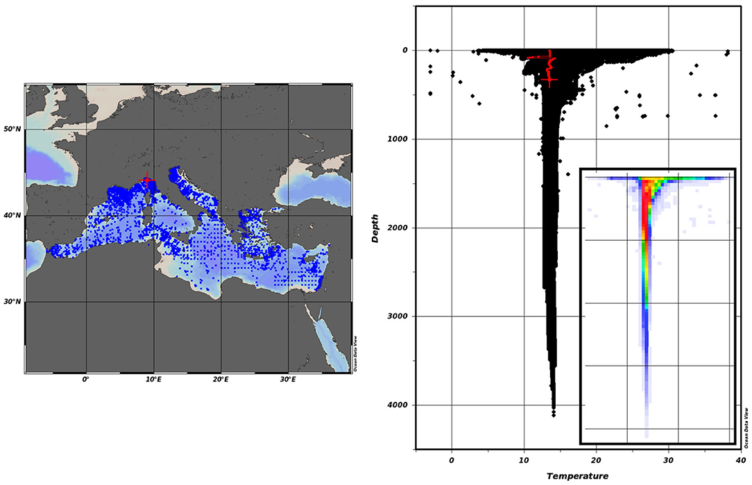
Figure 1. The data subset from the SeaDataCloud Mediterranean Sea data collection. Blue points (9, 293) on the map indicate the observed stations. The right scatter plot shows the strongly overlapping of more than 2, 000, 000 temperature measurements. The red line depicts a typical profile in the cloud containing good as well as bad data. The bottom right inlay figure shows the density of the samples.
Due to the overlapping, good and bad data cannot be separated in a two dimensional depth-temperature scatter plot as shown in Figure 1. The reason, why good and bad data samples overlap is that we are looking on data from different locations and environmental conditions, like for instance being close to the coast or in open waters. Further, we are looking on data from different seasons like summer and winter.
A high dimensional space is needed to distinguish the good and bad data. Ocean experts do not only inspect the depth-temperature space as seen in Figure 1, but they perform the analysis by sub-regions, depth layers or time periods to reduce the range of temperature variation. The experts analyze also water salinity and density distributions and evaluate different statistics. Another important feature to identify erroneous data is the temperature gradient, i.e., the change of temperature with depth (Simoncelli et al., 2018b). This is what we are exactly going to mimic with our DL algorithm.
3. Deep Neural Network Design
Our used data is extremely irregular. Data acquired in a single cruise are correlated in space and time, moreover our data set is characterized by different cruises or monitoring arrays, due to the combination of different types of measurements from different instruments. Our data vary in a 4D space (longitude, latitude, depth, and time). Thus there are measurements, which are very close in e.g., longitude, latitude, and depth, but one has been taken in winter, one in summer, or in different years. This yields also for the other dimensions, where we can have e.g., two measurement close in time, but at different locations. On top of this heterogeneity, the 4D space is irregularly sampled and profiles consist of different numbers of samples. Hence we decided to use a fully connected Multi-Layer-Perceptron (MLP) network architecture, because it is the most flexible and simultaneously simplest first approach, which can be applied to single samples making minimal assumptions on the data and the underlying mappings from input to output. Other neural network architectures exist, e.g., recurrent neural networks (RNN) or convolutional neural networks (CNN) and exploring their applicability to our problem is envisaged for the future, but beyond the scope of this work. The MLP is a deep learning neural network architecture consisting of an input layer including the so-called features, several hidden layers, each containing a certain number of nodes and the output layer, which in our case, for a binary classification problem consists of two output nodes.
Regarding the mentioned heterogeneity of the data one might argue that it would make sense to cluster the data into collections with similar features, e.g., a cluster containing only summer data at a specific location and depth, and then create AI algorithms specifically for all these clusters. While this is true to some degree, the problem is that we would have too few data in these clusters to train networks robustly. The training of one single network with all data yields the most robust and skillful results, thus we preferred generality over specificity, less accuracy but more robustness.
One of the most important aspects in machine learning are the input features for the algorithm, i.e., the information about our data we feed into the model. In our case we have started with the most basic and informative features listed in the following:
• Depth: The depth data.
• Temperature: The raw temperature data.
• Longitude: The longitudinal position.
• Latitude: The latitudinal position.
• Season: Month.
• Temperature gradient: The change of temperature with depth.
• Temperature gradient above: The gradient from the above sample.
• Temperature gradient below: The gradient from the below sample.
The temperature gradient is an important metric, because it gives additional information about the succession of the data and is sensitive to jumps or spikes in the data. After deciding to use the MLP approach and defining the input features, the size or complexity of the network has been chosen. In terms of hyper-parameter optimization (many different architectures have been tested) we found the best performance by using a fully connected network of 2 hidden layers with 128 and 64 nodes. This architecture fits well to the size of our dataset, the number of input features (8), the binary classification task and the complexity of the problem. Above we mentioned the flexibility of the MLP, however one important requirement to the MLP is that we need existing input features for each sample. Thus, at the boundaries of the profiles (top and bottom) we have no “Temperature gradients above/below” thus we used fill values in these cases.
4. Training and Tuning the Network
For the training of the network we use computing resources from AWI and TU Dresden and we use the Keras libraries7 for the implementation of the algorithm. For the sake of increasing the computational speed during the training phase we sub-sampled from the dataset all temperature profiles with at least one bad sample. Additionally we excluded profiles with more than 100 bad samples, which we consider as gross errors, which is not the target of SalaciaML. Thus, we reduced the dataset to 9, 293 profiles containing in total 2, 080, 698 samples. Regarding the dimensions of our fully connected network (2 hidden layers, 128 and 64 nodes each), with in total 128 * 64 = 8, 192 parameters (weights), we are dealing with a quite small network compared to the data, while often deep artificial neural networks have more parameters than data to be trained on, and still are skillful and generalize well (details e.g., in Zhang et al., 2016).
Following the sub-sampling we divided the dataset into four parts:
• Training data (55%): to be used to train the network
• Validation data (15%): to tune the data and avoid under/overfitting
• Testing data (10%): to tune the classification thresholds
• Control data (20%): to assess the skill of the model
A crucial aspect for partitioning the data is to keep profiles and distribute them into the four datasets without splitting themselves, although the MLP approach is not based on profiles and in the end, single data points can be fed into the model. The reason is that if we would destroy the profiles and separate the data samplewise, parts of a single profile can end up in all four datasets. This means that it would happen that we train the model with data from a certain space and time position and then evaluate it on data from the same space and time position, i.e., the model is trained and evaluated on the same profile. Of course it is not the exact same data, but data, which is much to strongly related to create a generalized model. The temperature profiles were distributed randomly but ensuring the geographic position to cover the whole region resembling their original distribution in all four datasets. However, data are non homogeneous in space and time, with more data in the northern than in the southern Mediterranean and the data availability decreases from shallow to the deep ocean.
The Keras library has been used for the training of the network with the ReLU (e.g., Glorot et al., 2010) as activation function/unit and the “Adam”8 optimizer with default settings. During the training the cross-entropy loss between the true labels and the predicted labels is minimized. The validation data is used to tune the model avoiding under- and over-fitting by optimizing the parameter called epoch number. This parameter defines the number of Keras learning iterations on the dataset. If the epoch number is set too low, we miss information during the training, if it is too high we overfit the data. This means that the network would start to misinterpret noise as a real feature, which is not desired. Therefore, we trained the dataset using epoch numbers from 1 to 200. Then we estimated the model loss on the “known” training dataset and the validation dataset which has not been used during the training, thus it is “unknown” to SalaciaML. The model loss indicates how close the model estimations are to the original data, thus the smaller the loss, the better the model. Figure 2A shows the loss for the training (blue) and the validation data (red). The longer the model learns on the training data the better are the estimations. This is because the model is evaluated on the same data it is trained with. The situation is different for “unknown” data, i.e., the validation dataset (red curves). First the loss is larger, which means that the model is of course less skillful on unknown data. Second, the model loss decreases (performance increases) only until approximately 125 epochs and then starts to increase again, where the model starts overfitting the data. Normally this point defines a stopping criterion for the training process. A common trick to increase the model skill is to use the dropout method suggested by Srivastava et al. (2014). The idea is a “thinning” of the network, i.e., after every epoch we ignore a certain percentage of the nodes randomly. Doing this, the model can learn longer without overfitting. Sensitivity tests have shown that we reach the best performance with a dropout of 20% and stopping the learning after 200 epochs, as shown in Figure 2B.
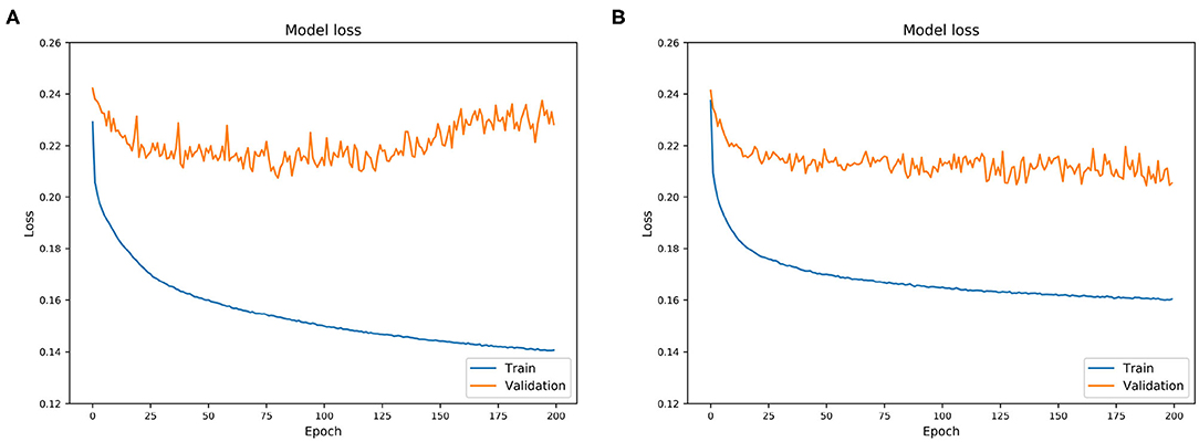
Figure 2. Loss plot with overfitting. Tuning the model by optimizing the epoch number. Blue curves: model evaluation on training dataset, red curves: evaluation on validation data. After each learning iteration (epoch) the model loss is reduced, i.e., the model learns: (A) Loss plot with overfitting. (B) Loss plot without overfitting. Using dropout for “thinning”.
Another important issue to deal with is the imbalance of our data set, i.e., we have 99% good and 1% bad data in the training set. The crucial point is that the Keras output layer provides for every sample a probability between 0 and 1 being good or bad. The default classification threshold is 0.5, which means classifying a sample as good if the probability is smaller than 0.5 and bad otherwise. This threshold yields very bad results for our imbalanced data set, because it simply does not account for the different weights of having much more good than bad data for the network training. The following approach has been adopted to deal with the imbalanced data. First we implemented an oversampling technique for the bad data, which means we exposed the bad data several times (15) to the algorithm to increase the weight of the bad data. Additionally we used the testing dataset (“unknown” to the algorithm) to generate the so-called ROC curve shown in Figure 3. We perform the classification for 6,000 thresholds between 0 and 1. For every classification we calculate the TPR (true positive rate), i.e., the fraction of good data classified correctly and the FPR (false positive rate), i.e., the fraction of bad data wrongly classified good and plot it as a blue dot in Figure 3. The area under the curve, the so-called AUC-value yields as a criterion for the skill of the classification with a maximum at unity. As can be seen in Figure 3, we observed a highly skillful AUC-value of 0.952, and a well-shaped ROC.
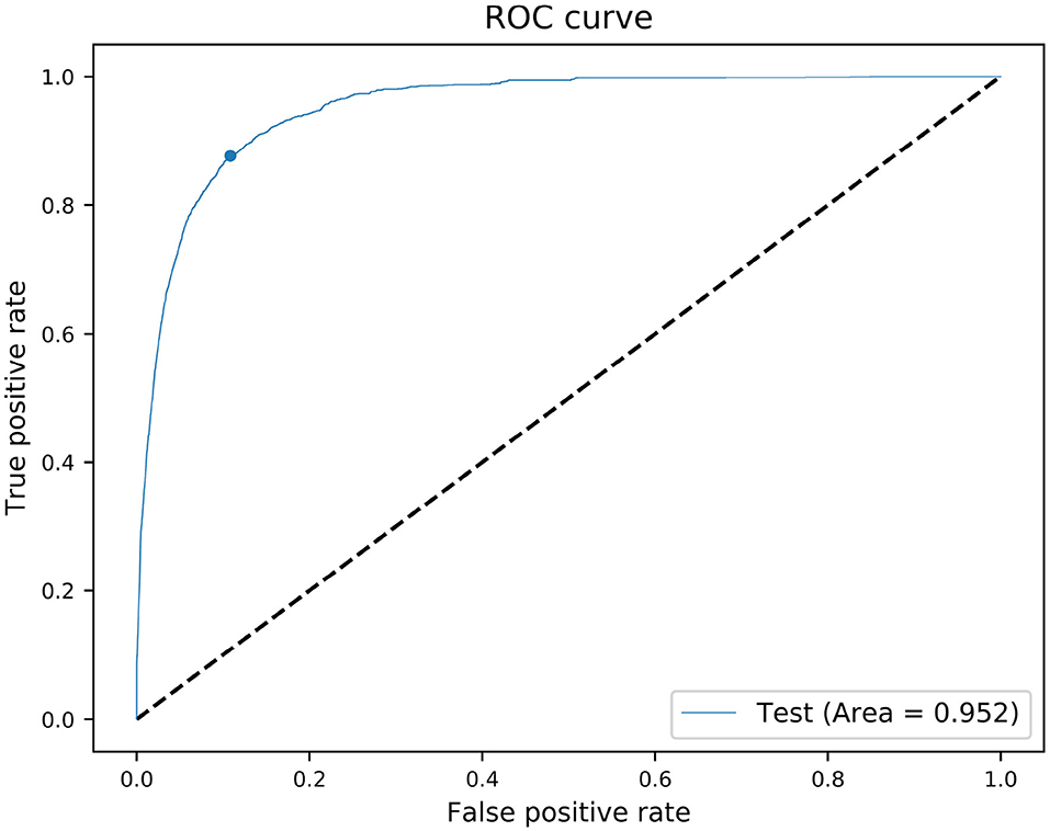
Figure 3. ROC diagram used to tune the classification threshold for our imbalanced dataset. The TPR and FPR of the model have been evaluated for 6,000 classification thresholds from 0 to 1 and the model skill is represented by the blue curve. The blue dot is the optimal classification threshold, found by maximizing the TPR and minimizing the FPR.
The optimum of the ROC is a point at TPR = 1, FPR = 0, AUC-value = 1, which means all good are flagged correctly and there are no bad flagged wrongly, which in turn means that all bad are correctly flagged. Every blue point of the curve in Figure 3 is related to a classification threshold, thus we can select the classification threshold corresponding to a ROC value as close as possible to the top left corner, which represents an objective optimum. However, other subjective choices can make sense, depending on the application of the classification method. There are two extremes of the ROC, i.e., the top right and the bottom left. If we select a classification threshold, which yields a ROC in the top right corner it means that we flag simply most data as good, which yields a very high TPR, but we are making a large error in flagging many bad falsely as good. In contrast a classification threshold, which gives a ROC in the bottom left corner means that we flag most of the data as bad, i.e., all bad data are truly flagged bad, but unfortunately also many good are flagged bad. Thus, the ROC metric can be used as a guideline to tune the algorithm to find the best compromise between TPR and FPR, i.e., correctly identifying as most as possible good, while making the smallest possible error in classifying bad as good by choosing the classification threshold yielding to the top left point of the ROC curve, which is for our data at 0.20 instead of the standard 0.50.
Summarizing we used the training dataset for the SalaciaML learning procedure, i.e., tuning the network weights. We used the validation dataset to find an optimum learning duration regarding under- and overfitting and we used the testing dataset to adjust the classification threshold to account for the imbalanced number of good and bad data. Additionally we used the dropout technique during the learning to increase the learning phase as well as an oversampling procedure to account for the imbalanced data. Accordingly we have to measure the skill of the tuned model with completely unseen data, the control dataset.
5. Results and Interpretation
To assess the skill of the model we use the control dataset (415, 961 samples), which again is “unknown” to SalaciaML. Figure 4 shows the obtained results. The top left panel of Figure 4 depicts the real bad data, i.e., the original truth from the control dataset. The top right panel shows the bad data classified by SalaciaML. The two bottom panels show the real (left) and predicted (right) good data. The color scale indicates the density of the samples, where each panel presents different axes ranges. Thus, the density pattern of good and bad can be compared visually. The shape and density of the estimated flags agree astonishing well with the original patterns. While the absolute numbers of the good flags are very similar for the original and estimated flags, SalaciaML finds 10 times more bad classifications than actually existing in the control dataset.
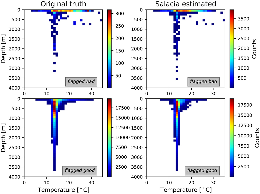
Figure 4. SalaciaML results: (top left) the original bad flagged samples; (top right) the estimated bad samples; (bottom left) the original good samples; (bottom right) the estimated good. The color scale indicates the density of the overlapping samples.
The skillful classification strength of SalaciaML applied to the Mediterranean Sea is substantiated by the estimated confusion matrices9 in Table 1.
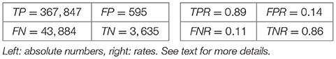
Table 1. Confusion matrices for the optimal threshold in the control dataset.
The table on the left of Table 1 depicts the absolute numbers of true positive estimates (TP), false positives (FP), true negatives (TN), and false negatives (FN), while the right table shows the true positive rate (TPR), i.e., the fraction of good data classified correctly, the true negative rate (TNR), i.e., the fraction of bad data correctly classified, the false positive rate (FPR) which is the fraction of bad data wrongly classified good and the false negative rate (FNR) describing the fraction of good data wrongly classified as bad. The confusion matrices indicate a high overall skill of SalaciaML detecting most good and bad samples. However, the imbalance of the data, i.e., much less bad than good data, should be kept in mind for real applications of SalaciaML. Considering the results in Table 1 one possible option for real QC applications could be that the QC experts accept the good flagged data and perform a post-QC, visually on the bad flagged data, which represent only ca. 11% of the data, i.e., (43, 884 + 3, 635)/415, 961 = 0.114 to create a highly correct data product. However, the discussion on operational applications of SalaciaML is beyond the scope of this study and will be left to follow up projects.
Since the data are non homogeneously distributed over the Mediterranean domain, the skill of the model has been assessed in 16 regions (Figure 5), following the approach of Simoncelli et al. (2018b). We applied SalaciaML to 16 regional control datasets. We must recall that our algorithm has been trained and tuned with the full Mediterranean training/validation/testing datasets to benefit from being robust and general. And that it can be applied to any data from the Mediterranean, even single profiles or single samples. As also mentioned in section 3, one might argue that it could make sense to train and tune 16 individual networks, one for each region. However, we tested this approach and it turned out that we have not enough data samples in the individual regions to train and tune these models robustly. Figure 5 shows the results per sea regions. The accuracy is shown on the y-axis, while the 16 regions are indicated on the x-axis. Green bars show the TPR, i.e., the accuracy for the good samples and the red bars show the TNR, the accuracy for the bad samples.
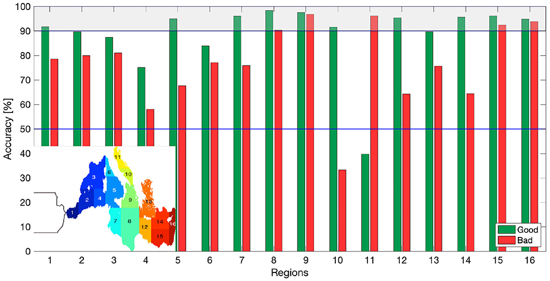
Figure 5. Regional skill assessment. The accuracy for the estimation of the good (green) and the bad (red) samples for 16 Mediterranean regions.
SalaciaML is both skillful and generalizes well. Most regions show skills in the order of 80–90%, with skills larger than 90% in 11 out of 16 regions. Especially high skill for both (good and bad) is observed in regions 8, 9, 15, and 16. All other regions show moderate skills between 70 and 90%, except for region 11 (Northern Adriatic), having a weak accuracy for the good detection and region 10 (Southern Adriatic) with a weak accuracy for the bad classification.
6. Significance Considerations
Ocean data skill assessments on sample basis are rare, which makes it difficult to compare the accuracy observed by SalaciaML with other methods. Even for methods based on full profiles very few skill analyses exist. One prominent study, already mentioned in the introduction, is that of Gronell and Wijffels (2008), who developed the QuOTA system. Their results of applying automatic QC algorithms are not directly comparable with our study because they classify profiles as bad if they find at least one bad sample within the profile, but still gives a considerable understanding of the possibilities of state-of-the-art algorithms. Nevertheless the general behavior of QuOTA and SalaciaML is quite similar. QuOTA finds 95.5% of all bad profiles, but at the same time classifies 17% of the profiles wrongly bad. In relation to these numbers we found in total a TNR = 86% and FNR = 11% (cf. Table 1). In some Mediterranean regions we even found TNR > 90% and FNR < 10% (cf. Figure 5). Both SalaciaML and QuOTA are quite skillful in detecting bad data on the drawback of being too sensitive, which is understandable, because both are trained to find those bad data. This comparison shows that both algorithms “play in the same league,” nevertheless we have to keep in mind the slightly different approaches of SalaciaML and QuOTA for interpretation of the results. Regarding the fact that SalaciaML is a first approach, where we started with a basic set of input features and with basic model optimizations we see a strong potential for improvements in follow up projects.
Additionally to comparisons with already existing methods it is crucial to estimate the significance of the algorithm itself. The main reason for that is to exclude e.g., faults in the data, the experiment or algorithm. To make it clear we want to rule out that our algorithm reached the observed skill by chance. Therefore, we performed a few simple significance tests to further assess the skill observed with SalaciaML. A typical approach in significance testing is to set up a null-hypothesis or null-model and the results are tested against it. We applied three different null-models to our data and compared their skill to the one of SalaciaML.
1. Flag all good: A naïve classification is simply to flag all data as good. The overall accuracy is very high (99%), however this result is trivial, because of the imbalanced data, i.e., 99% good and 1% bad. Hence, this approach yields 100% accuracy for the good it gives 0% accuracy for the bad. It is clear that this approach is useless.
2. Flag all random: A very useful check of a statistical method is to test its performance on randomized data or behavior. This test accounts for the skill, which can be more or less achieved by chance. We assigned the flags good and bad simply randomly to each sample. As expected we achieve high accuracy (> 95%) for the good, but very weak skill in the order of 10% for the bad.
3. Split depths: A more sophisticated null-model takes into account prior knowledge on the QCed data and the SalaciaML results. Most of the originally flagged bad data are located in the upper ocean. Similarly SalaciaML flags mostly bad data in the upper layer. Thus, regarding the fact that not much more than flagging 10% of the whole data bad is tolerable, because of the false negatives, we flag the upper 10% of each profile bad and the rest good. This resembles the proportion of good and bad found by SalaciaML. It turned out that the accuracy for the good is in the order of 90% and the accuracy for the bad ranges between 20 and 50%. The example shows that this null-model has indeed a skill, which is different from random chance. Still the skill for the bad is not acceptable and far below the skill provided by SalaciaML.
Our rough significance considerations show that the observed results found by SalaciaML are far from being random or trivial. They are even much more skillful than a null-model, which takes into account some prior knowledge on the distribution of good and bad data. Thus, we can clearly say that the skill of SalaciaML, mostly between 80 and 95% for both, good and bad is significant and cannot be achieved easily without sophisticated methods.
7. Summary and Conclusions
In the framework of the EU SeaDataCloud project we have trained a deep learning artificial neural network with more than 2, 000, 000 temperature measurements over the Mediterranean Seas spanning the last 100 years. The goal of the DL algorithm SalaciaML is to support the small scale visual QC performed by ocean experts. While semi-automated classical procedures like range checks help to identify the gross errors in the data, not enough skillful algorithms are available to detect erroneous small scale features, requiring to check profile by profile and sample by sample. SalaciaML is able to support in this difficult and time-consuming QC task highlighting the erroneous small scale features by assigning a bad quality flag to suspicious data. Thus, SalaciaML gives hints to samples, which could be bad and it is up to the QC expert to judge on these suggestions. SalaciaML reaches high accuracies larger than 90% in identifying good or bad data in many regions of the Mediterranean Sea, which makes it especially useful in these regions. However, regarding the typical imbalance of Mediterranean temperature profiles, i.e., much more good than bad data, we recommend that the QC experts concentrate on using only the SalaciaML bad flags as a guidance and accept the SalaciaML good. This results in checking only ca. 10% of the data. However, since the SalaciaML flags are widely distributed among profiles, the QC experts have still to check all profiles containing measurements flagged as bad. The crucial workload reduction consists of supporting the QC by giving hints to potentially bad data on the small scale temperature features, which was not possible with acceptable skill until now, and might help to find bad data, which had been overlooked otherwise.
The development of SalaciaML represents one of the first applications of AI (together with e.g., Leahy et al., 2018; Castelao, 2020) and deep learning for massive ocean data quality control. We used a quite standard approach in deep learning with a fully connected MLP architecture. To tune the network we optimized several hyperparameters and accounted for the imbalance of the data by oversampling and ROC classification threshold optimization. The implemented setup, together with the availability of a validated data collection, allowed SalaciaML to reach satisfactory skills which make it helpful and supportive during the QC procedure. From this experience we think that there is quite a room for improvements, like testing other network architectures, including more input features and optimizing hyperparameter in more depth.
We started using the most known and available Ocean Essential Variable, i.e., sea temperature, but it would be crucial to test this application to other variables, such as salinity, oxygen, nutrients like nitrate, phosphate, silicate, metals, and much more. In fact all these variables act together in complex interactions, which involves both physical and biogeochemical processes. In the case of a lack of certain data, promising methods exist to estimate missing data as shown by Sauzéde et al. (2017). The inclusion of these diversity and manifoldness into a deep learning system is a challenge, but the field of artificial intelligence could be the way to handle this complexity.
Our methodology is far away from being operational and more real applications are now needed to improve performance and learn for an envisaged operational setup. These efforts are now started together with the SeaDataNet QC community and our long-term goal is to setup an operational service, providing SalaciaML to the benefit of global ocean data and the science community. As an additional outlook it is planned to explore the possibilities of SalaciaML to separate “pure” good profiles from profiles with at least one bad sample as followed by the IQuOD community. Further hybrid approaches of combining different SalaciaML setups or including classical pre-processing are envisaged to be investigated in follow up projects.
Data Availability Statement
Publicly available datasets were analyzed in this study. This data can be found at: https://doi.org/10.12770/2698a37e-c78b-4f78-be0b-ec536c4cb4b3.
Author Contributions
SM, SD, RS, and SSe designed the research. SD performed the research with help from SM and SSe. SSi provided help regarding the classical quality control procedures. SM wrote the manuscript with contributions from SD, SSi, and SSe. All authors contributed to the article and approved the submitted version.
Funding
This project has received funding from the European Union Horizon 2020 and Seventh Framework Programmes under grant agreement number 730960 SeaDataCloud.
Conflict of Interest
The authors declare that the research was conducted in the absence of any commercial or financial relationships that could be construed as a potential conflict of interest.
Acknowledgments
We thank Peter Steinbach from the HZDR (Helmholtz-Zentrum Dresden-Rossendorf) for organizing the Dresden Deep Learning Hackathon 201910. Participation in the Hackathon boosted this work significantly. We are very thankful to our colleagues from the AWI computing center, especially Jörg Matthes for the provision of VM's for training our algorithm. Additionally we thank Axel Behrendt for discussions on classical ocean data quality control.
Footnotes
2. ^https://cdi.seadatanet.org/search
5. ^https://odv.awi.de/fileadmin/user_upload/odv/misc/ODV_QualityFlagSets.pdf
6. ^https://www.seadatanet.org/Products/
8. ^https://keras.io/api/optimizers/adam/
References
Behrendt, A., Sumata, H., Rabe, B., and Schauer, U. (2018). Udash-unified database for arctic and subarctic hydrography. Earth Syst. Sci. Data 10, 1119–1138. doi: 10.5194/essd-10-1119-2018
Boyer, T. P., Baranova, O. K., Coleman, C., Garcia, H. E., Grodsky, A., Locarnini, R. A., et al. (2018). World Ocean Database 2018. National Center for Environmental Information.
Bushnell, M., Waldmann, C., Seitz, S., Buckley, E., Tamburri, M., Hermes, J., et al. (2019). Quality assurance of oceanographic observations: standards and guidance adopted by an international partnership. Front. Mar. Sci. 6:706. doi: 10.3389/fmars.2019.00706
Castelao, G. P. (2020). A framework to quality control oceanographic data. J. Open Source Softw. 5:2063. doi: 10.21105/joss.02063
Glorot, X., Bordes, A., and Bengio, Y. (2010). “Deep sparse rectifier neural networks,” in Proceedings of the Fourteenth International Conference on Artificial Intelligence and Statistics, Vol. 15 (Fort Lauderdale, FL).
Gourrion, J., Szekely, T., Killick, R., Owens, B., Reverdin, G., and Chapron, B. (2020). Improved statistical method for quality control of hydrographic observations. J. Atmos. Ocean. Technol. 37, 789–806. doi: 10.1175/JTECH-D-18-0244.1
Gronell, A., and Wijffels, S. (2008). A semiautomated approach for quality controlling large historical ocean temperature archives. J. Atmos. Ocean. Technol. 25, 990–1003. doi: 10.1175/JTECHO539.1
Leahy, T. P., Llopis, F. P., Palmer, M. D., and Robinson, N. H. (2018). Using neural networks to correct historical climate observations. J. Atmos. Ocean. Technol. 35, 2053–2059. doi: 10.1175/JTECH-D-18-0012.1
Sauzéde, R., Bittig, H. C., Claustre, H., Pasqueron de Fommervault, O., Gattuso, J.-P., Legendre, L., et al. (2017). Estimates of water-column nutrient concentrations and carbonate system parameters in the global ocean: a novel approach based on neural networks. Front. Mar. Sci. 4:128. doi: 10.3389/fmars.2017.00128
Schlitzer, R. (2002). Interactive analysis and visualization of geoscience data with ocean data view. Comput. Geosci. 28, 1211–1218. doi: 10.1016/S0098-3004(02)00040-7
Simoncelli, S., Fichaut, M., Schaap, D., Schlitzer, R., Barth, A., and Fratianni, C. (2019). “Marine Open Data: a way to stimulate ocean science through EMODnet and SeaDataNet initiatives,” In: INGV Workshop on Marine Environment, Vol. 51, eds L. Sagnotti, L. Beranzoli, C. Caruso, S. Guardato, and S. Simoncelli (Rome), 1126. Available online at: http://editoria.rm.ingv.it/miscellanea/2019/miscellanea51/
Simoncelli, S., Myroshnychenko, V., and Coatanoan, C. (2018b). SeaDataCloud Temperature and Salinity Historical Data Collection for the Mediterranean Sea (Version 1). Product Information Document (PIDoc). doi: 10.13155/57036
Simoncelli, S., Schaap, D., and Schlitzer, R. (2018a). Mediterranean Sea - Temperature and salinity Historical Data Collection SeaDataCloud V1. [dataset]. doi: 10.12770/2698a37e-c78b-4f78-be0b-ec536c4cb4b3
Srivastava, N., Hinton, G., Krizhevsky, A., Sutskever, I., and Salakhutdinov, R. (2014). Dropout: a simple way to prevent neural networks from overfitting. J. Mach. Learn. Res. 15, 1929–1958.
Keywords: deep learning, Keras, quality control, SeaDataNet, ocean data view, ocean temperature profiles
Citation: Mieruch S, Demirel S, Simoncelli S, Schlitzer R and Seitz S (2021) SalaciaML: A Deep Learning Approach for Supporting Ocean Data Quality Control. Front. Mar. Sci. 8:611742. doi: 10.3389/fmars.2021.611742
Received: 29 September 2020; Accepted: 10 March 2021;
Published: 28 April 2021.
Edited by:
Hervé Claustre, Centre National de la Recherche Scientifique, FranceReviewed by:
Guillaume Maze, Institut Français de Recherche pour l'Exploitation de la Mer, FranceFabien Roquet, University of Gothenburg, Sweden
Copyright © 2021 Mieruch, Demirel, Simoncelli, Schlitzer and Seitz. This is an open-access article distributed under the terms of the Creative Commons Attribution License (CC BY). The use, distribution or reproduction in other forums is permitted, provided the original author(s) and the copyright owner(s) are credited and that the original publication in this journal is cited, in accordance with accepted academic practice. No use, distribution or reproduction is permitted which does not comply with these terms.
*Correspondence: Sebastian Mieruch, c2ViYXN0aWFuLm1pZXJ1Y2hAYXdpLmRl