Characterizing Community Structure of Benthic Infauna From the Continental Slope of the Southern California Bight

Gillett, David J.; Gilbane, Lisa; Schiff, Kenneth C.

doi:10.3389/fmars.2021.605858

ORIGINAL RESEARCH article

Front. Mar. Sci., 28 January 2021

Sec. Marine Ecosystem Ecology

Volume 8 - 2021 | https://doi.org/10.3389/fmars.2021.605858

Characterizing Community Structure of Benthic Infauna From the Continental Slope of the Southern California Bight

$\r\nDavid J. Gillett*$ David J. Gillett^1*

Lisa Gilbane²

Kenneth C. Schiff¹

¹Southern California Coastal Water Research Project, Costa Mesa, CA, United States
²Environmental Analysis Section, Bureau of Ocean Energy Management, Camarillo, CA, United States

Infauna are an ecologically important component of marine benthic ecosystems and are the most common faunal assemblage used to assess habitat quality. Compared to the shallower waters of the continental shelf, less is known about the benthic fauna from the continental slope, especially how the communities are structured by natural gradients and anthropogenic stressors. The present study was conceived to rectify these data gaps and characterize the natural, baseline structure of the benthic infauna of the upper continental slope (200–100 m) of the Southern California Bight. We aggregated benthic infauna, sediment composition, and sediment chemistry data from different surveys across the Southern California Bight region (750 samples from 347 sites) collected between 1972 and 2016. We defined 208 samples to be in reference condition based upon sediment chemistry and proximity to known anthropogenic disturbances. Cluster analysis of the reference samples was used to identify distinct assemblages and the abiotic characteristics associated with each cluster were then used to define habitat characteristics for each assemblage. Three habitats were identified, delineated by geography, depth, and sediment composition. Across the habitats, there were detectable changes in community composition of the non-disturbed fauna through time. However, the uniqueness of the habitats was persistent, as the fauna from each habitat remained taxonomically distinct from irrespective of the decade of their collection. Within each habitat, subtle, assemblage-scale responses to disturbance could be detected, but no consistent patterns could be identified among the component taxa. As with the non-disturbed samples, there were compositional changes in the fauna of the disturbed samples through time. Despite the changes, fauna from disturbed and non-disturbed samples remained taxonomically distinct from each other within each decade of the dataset. After considering both the spatial and temporal patterns in the fauna of slope ecosystem, it became apparent that there was a high degree of stochasticity in the taxonomic organization of all three habitats. This would suggest that the benthic fauna from these communities may be neutrally organized, which in turn poses interesting challenges for future development of condition assessment tools based upon the benthic fauna in these habitats.

Introduction

Benthic infauna are a key ecological component of nearly all marine ecosystems. They represent a key trophic link between organic matter production/accumulation in the benthic environment and export to other oceanic environments (Chardy and Dauvin, 1992; Kovecses et al., 2005; Wolkovich et al., 2014). The tube-building and bioturbation activities of the infauna also stimulate the productivity of the microbial community and enhance biogeochemical cycling (e.g., Michaud et al., 2006; Quintana et al., 2011; Laverock et al., 2014).

Benthic infauna are also the most common faunal assemblage used to assess habitat quality across the globe (e.g., Diaz et al., 2004; Llansó et al., 2009; Environmental Protection Agency, 2012) due to their sessile lifestyle, taxonomic diversity, and ability to integrate stressor exposure over time (e.g., Warwick, 1988; Dauer, 1993; Gray et al., 2002). A byproduct of the broad taxonomic and functional diversity of a typical marine benthic assemblage is an equally broad range in sensitivities to different types of stressors (e.g., Statzner and Bêche, 2010; Oug et al., 2012; DeLong et al., 2018). These characteristics combine to make for relatively predictable community-scale changes in both structure and function when exposed to disturbance (e.g., Pearson and Rosenberg, 1978; Rhoads et al., 1978).

In the coastal waters of southern California, the vast majority of the research and monitoring of macrobenthic infauna has occurred in the relatively shallow continental shelf, coastal embayments, and estuaries (Ward and Mearns, 1979; Ranasinghe et al., 2012; Schiff et al., 2016). The fauna of these shallower components of the coastal ocean are relatively well understood with respect to their biogeography and their response to anthropogenic disturbance (e.g., Smith et al., 2001; Ranasinghe et al., 2005, 2009). These patterns are important for managers and regulatory agencies to understand, because these waters are adjacent to a densely populated metro-center¹ and receive point source and non-point source discharges from more than 23 million people (e.g., County Sanitation Districts of Los Angeles County, 2016; City of San Diego, 2017; Orange County Sanitation District, 2017).

Comparatively less work has been done surveying and analyzing the patterns of the benthic fauna from the deeper waters of southern California’s continental slope and deep basin ecosystems. There have been a number of smaller-scale studies focused on the impacts of the persistent oxygen minima zones that occur in some of the isolated deep water basins of the Southern California Bight (e.g., Thompson et al., 1993; reviewed in Levin, 2003), but most do not provide regional-scale insights into the resident infauna, nor do they provide insight into anthropogenic disturbance to the system. The first truly comprehensive study of the region’s deep waters was reported by Hartman and Barnard (1958, 1960). The primary focus of their work was exploratory and to create a taxonomic inventory of the region’s deep-water fauna: yielding a number of new species descriptions and producing valuable dichotomous keys for identification of the fauna (Hartman and Barnard, 1960). A key conclusion of Hartman and Barnard was that the continental slope and deep basins of the Southern California Bight were a relatively homogeneous expanse, with a sparse infaunal community dominated by chaetopterid and serpulid polychaetes. Additionally, the United States Bureau of Land Management conducted a survey of the region’s deep water habitats in 1977² (Bureau of Land Management, 1978) and some surveys north of the region (Lissner et al., 1986; Hyland et al., 1991) describing infaunal communities as a function of the environment, including the impacts of oxygen minima zones. Useable records of the benthic infauna data produced from these surveys were not available to us at the time of the present study.

There has been a considerable maturation and technical advancement in the science of benthic ecology since the 1950s–1960s and the lack of a comprehensive synthesis of the resident fauna of the continental slope of southern California represents a distinct gap in our understanding of the status and health of the region’s coastal ocean. The outer continental shelf and continental slope represent more than 60% of the benthic habitat in the region (Gillett et al., 2017) and are the biological and sedimentary link from the continental margins to the deep basins and abyssal plain of the open ocean. Though relatively separated from the centers of human population, the deeper portions of the continental margins are still exposed to a variety of human disturbance pressures (e.g., Montagna and Harper, 1996; Terlizzi et al., 2008; Ellis et al., 2012). The continental shelf and slope of southern California are bisected by a number of submarine canyons that are thought to serve as potential conduits of contaminated sediments from the highly urbanized rivers, wastewater discharges, and waters of the near-shore to the deeper parts of the continental slope and basins (e.g., Palanques et al., 2008; Jesus et al., 2010; Bight ’13 Contaminant Impact Assessment Planning Committee, 2017). The continental slope is an important area for mineral, petroleum, and natural gas extraction, which can have deleterious impacts on resident benthic fauna (e.g., Olsgard and Gray, 1995; Manoukian et al., 2010; Ellis et al., 2012). Furthermore, these deeper waters experience the commercial trawling of demersal fishes and invertebrates (United States Geological Survey, 2016), which can also directly or indirectly (physical disturbance or by-catch) impact benthic infaunal community composition (Gislason et al., 2017; Ashford et al., 2018; Rijnsdorp et al., 2018).

Given the variety of anthropogenic pressures to the continental slope ecosystem at local (i.e., sewage outfalls, petroleum extractions, and physical disturbance) or region-wide (i.e., ocean acidification and climate change) scales, local, state, and federal management agencies have expressed a desire to quantify the nature and magnitude of any potential impacts in slope ecosystems, as can be done in shallower waters (Gillett pers comm). Unfortunately, at the present moment there is no accepted condition assessment framework for deeper waters of the region. The first steps in developing such a framework are to identify the best biotic components to focus on, quantify their variability along natural environmental gradients, and then identify any quantitative and repeatable responses to anthropogenic disturbances.

Having outlined a number of reasons why benthic fauna make a good focal point for the development of an assessment framework above, the next logical step is to proceed with quantifying regional-scale natural variability. Without an understanding of the community structure of the resident infauna of the southern California continental slope, we have no insight into the natural baseline structure and function of this environment. It is unclear if the whole of the system is a single contiguous habitat, as suggested by Hartman and Barnard (1960), or if there is some degree of community differentiation based upon biotic or abiotic factors.

The primary goals of this study were to characterize the natural, baseline structure of the benthic infauna of the continental slope of the Southern California Bight; to determine if there were discrete communities of fauna and if there were abiotic differences associated with those communities. A secondary goal was to determine if community or single-taxon responses to anthropogenic disturbance could be quantified for the future development of bioassessment indices and frameworks.

Materials and Methods

Analytical Approach

Macrobenthic infauna (i.e., those retained on 1 mm sieve), sediment composition, and sediment chemistry data were aggregated from different surveys across the Southern California Bight region collected between 1972 and 2016, with the largest share of data collected from the mid 1990’s through the 2010’s. Reference conditions were defined using sediment chemistry, proximity to known anthropogenic disturbances (e.g., oil/gas platforms and canyon mouths), and incidences of low species richness (an indicator of a poorly collected sample or an area of frequent hypoxia/anoxia). Cluster analysis of taxon-specific abundance data was used to identify distinct biotic assemblages. The abiotic characteristics associated with the samples from each cluster were then used to define habitat characteristics for each assemblage. Within each habitat, infaunal data were analyzed with a combination of univariate and multivariate techniques to identify any potential changes in assemblage composition with exposure to different levels of anthropogenic disturbance. Lastly, given the multi-decadal nature of the dataset, the potential influence of changes in the baseline benthic community (e.g., Gillett et al., 2017; Hale et al., 2018) on habitat delineation and stressor response needed to be investigated. The persistence of different benthic assemblages and habitats across the time frame of the dataset was evaluated by comparing biotic and abiotic variables at reference condition sites from each decade of samples to each other. Similarly, the ability to distinguish potential anthropogenic impacts on the biota through time was evaluated by comparing the relative differences in community composition between reference and non-reference condition samples within each decade to those from other time periods.

Datasets

The area of focus was the continental slope of the Southern California Bight (Figure 1). The region roughly extends from the United States – Mexico border northwards to Point Conception, California and between the mainland of the continent in the east to the Channel Islands in the west. Nominal depth boundaries were set at 200 m for the shallowest samples (approximate breakpoint between the outer continental shelf and the upper continental slope) and 1,000 m for the deepest samples (approximate sampling limitation of local research vessels). This is an area oceanographically influenced at shallower depths by the cold-water California Current flowing to the south mixing with the warm-water Davidson Countercurrent flowing to the north (Bray et al., 1999), as well as seasonal upwelling of nutrient-rich water (Chhak and Di Lorenzo, 2007). At depths below 300–400 m, the region is influenced by the northward flowing California Bottom Current, which transports relatively warmer, low oxygen Pacific Equatorial bottom water along the continental slope (e.g., Thomson and Krassovski, 2010). The relative magnitude and flux of this current has been observed to vary through time (Bograd et al., 2019).

FIGURE 1

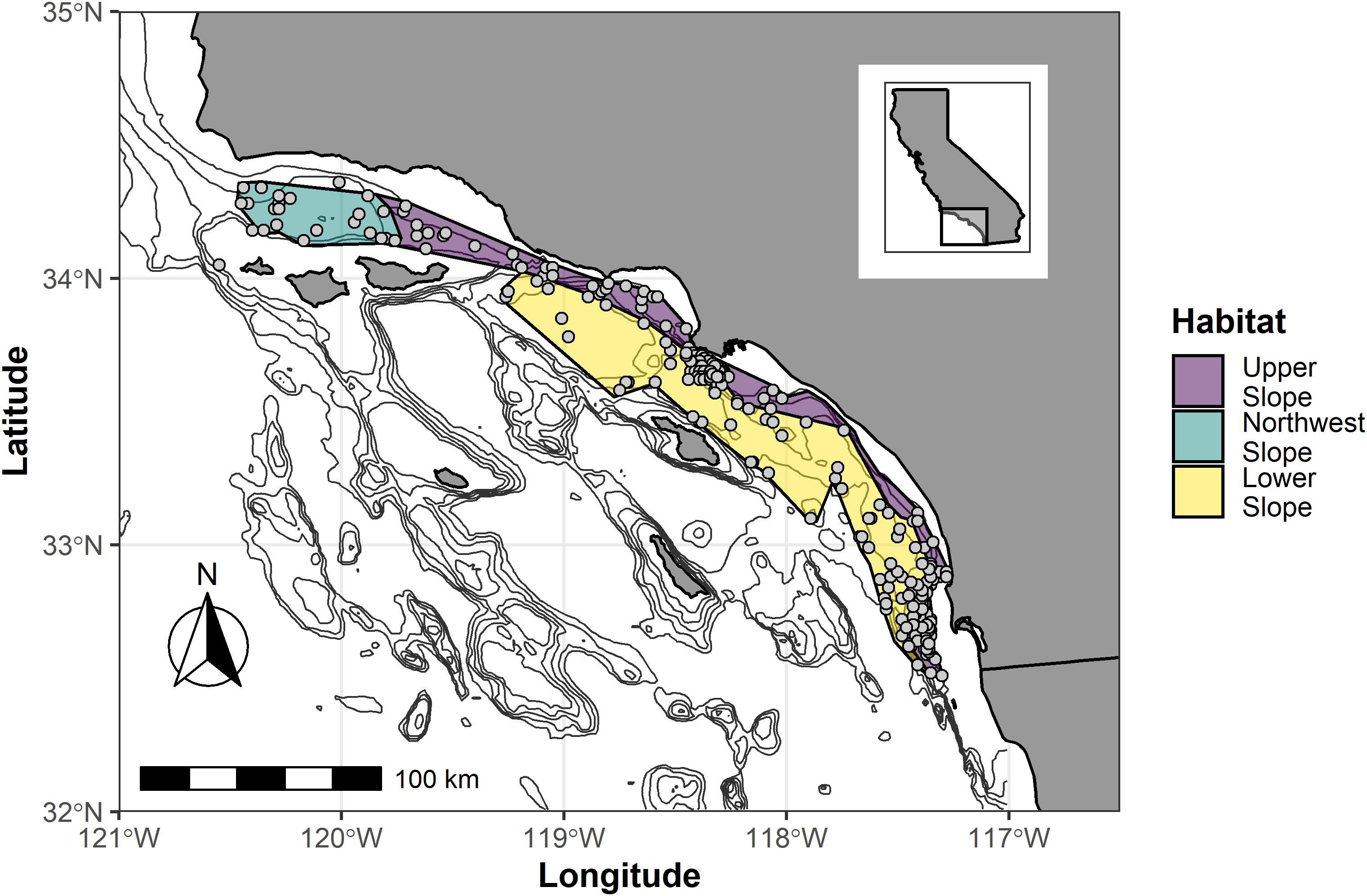
Figure 1. Map of the Southern California Bight depicting the location of benthic samples collected from the continental slope. The gray dots represent samples used in the study. Polygons represent the approximate boundaries of the three different habitats that were identified from biological differences among the reference samples (Figure 2). The black lines represent 200-m isobaths between 200 m and 1,000 m deep. The inset illustrates the location of the study area along the Pacific coast of California.

The sediment and infaunal data used in this study were obtained from four primary sources (Table 1) – a mix of fixed monitoring sites, probabilistic surveys, and special studies. We aggregated benthic grab samples collected during the summer (June 01 – September 30) from 1972 to 2016. Samples ranged in depth from 202 to 1,023 m. Eleven sites, with grabs collected from 1972 to 2015 (412 grabs) were at fixed locations along the ∼304 m isobath of the Los Angeles County Sanitation Districts’ monitoring grid. The remaining sites were sampled only once between 1997 and 2016 as part of the Southern California Bight Regional Monitoring Program (Schiff et al., 2016) (228 grabs) or limited special studies conducted by the local sanitation districts (95 grabs) (Table 1). From these datasets, we extracted information on benthic infaunal identity and abundance, sediment grain size composition, and sediment chemistry. Targeted chemistry parameters included total organic carbon (TOC), total nitrogen (TN), metals, poly-cyclic aromatic hydrocarbons (PAHs), poly-chlorinated biphenyls (PCBs), and Dichlorodiphenyltrichloroethane (DDTs). These chemistry measures consist of a mix of purely anthropogenic compounds (e.g., DDTs or PCBs) that were historically introduced to the environment via wastewater and the movement of contaminated sediments (Niedoroda et al., 1996; Zeng and Venkatesan, 1999), as well as naturally occurring compounds that can be concentrated by human activities and delivered to the environment (e.g., metals, PAHs, or TOC).

TABLE 1

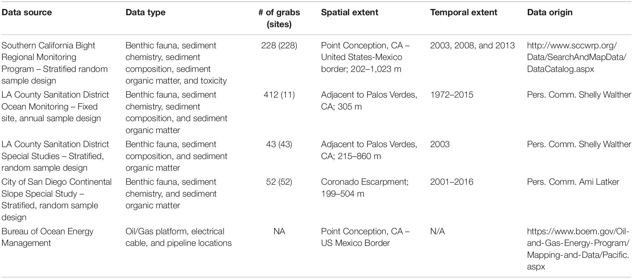
Table 1. Inventory of data used in this study.

The majority of the samples were collected with a 0.1 m² modified Van Veen grab. Samples from the Los Angeles County Sanitation Districts collected before 1980 (i.e., eight sampling events at 11 sites) were collected as four replicate 0.04 m² Shipek grabs. Given the smaller sample area of these older samples, benthic data from the first three replicate samples were summed together to approximate the samples collected with the Van Veen grab post-1980 – an approach developed by the Los Angeles County Sanitation Districts (S. Walther, pers. comm.). Most of the sampling programs that served as data sources for the present study only collected a single replicate grab for faunal or chemistry data. Consequently, with all post-1980 data, if more than one replicate grab was collected only data from the first replicate sample were used in the final analytical dataset to minimize overweighting the influence of samples from a limited spatial area and time frame within our regional analyses. The final dataset consisted of 750 samples from 347 sites.

Sample grabs for infauna were sieved on a 1-mm screen and fixed in buffered formalin. Infaunal taxonomy was standardized to SCAMIT edition 11 (Southern California Association of Marine Invertebrate Taxonomists, 2016), and ambiguous taxa were aggregated to higher taxonomic levels on a sample-wise basis. The dataset contained 1,198 distinct macrobenthic taxa from 15 different phyla. Of the 750 infaunal samples, 86% had synoptically collected sediment chemistry, 83% had sediment grain size, and 80% had measures of TOC or TN.

Based on analogous studies in shallower depths and interactions with local experts, reference criteria were established to identify a group of minimally disturbed reference sites (sensu Stoddard et al., 2006). Both natural and anthropogenic forcing factors can influence biotic community composition. By establishing reference criteria and the subsequent identification of reference condition sites, one can characterize any “natural” differences in community composition due to biogeography and other basin-scale factors (e.g., ENSO/PDO, waxing and waning of dominant currents) without the confounding influence of any potential local anthropogenic disturbance. The following six filters were used as our reference criteria: (1) sites had to be >3 km from an oil/gas platform (e.g., Olsgard and Gray, 1995; Ellis et al., 2012); (2) sites had to be >3 km from submarine canyon mouths; (3) no sites could be within the zone of influence of the Los Angeles County Sanitation Districts’ Palos Verdes treated effluent outfall (County Sanitation Districts of Los Angeles County, 2016); (4) samples could contain no more than 5 chemicals with concentrations greater than their associated Chemical Score Index (CSI) Minimal Exposure threshold (Bay et al., 2014); (5) samples could contain no chemicals with concentrations greater than their associated CSI Low Exposure threshold (Bay et al., 2014); (6) no samples with less than 5 taxa.

The first three criteria are spatial filters to exclude areas with the potential to accumulate contaminants. The next two filters are based on the Chemical Score Index (CSI), an assessment tool used by the State of California to assess the potential toxic effects of eight individual contaminants, plus the sum concentrations of PCBs, low molecular weight PAHs and high molecular weight PAHs on benthic infauna of the region. CSI Minimal Exposure thresholds are concentrations below which impacts to the biota are not expected. CSI Low Exposure thresholds are concentrations above which impacts are likely to occur. The sixth filter focused on minimum number of taxa, which could be indicative of impacts from unmeasured stressors (e.g., low dissolved oxygen) or of a poor-quality sampling event.

Biological Assemblages

Once a group of reference sites was identified, the possibility of distinct biotic assemblages and then possibly distinct abiotic habitats associated with those assemblages were evaluated by looking for taxonomic similarities and differences among the samples via clustering the infauna sample data from the reference sites. Taxonomic similarity was quantified as Bray–Curtis dissimilarity values (Bray and Curtis, 1957). To maximize the formation of meaningful clusters of samples, dissimilarities were calculated with taxa at three different levels of taxonomic specification: species and above, genus and above, or family and above (Supplementary Material 1). A genus-level identification was selected to move forward with, as it produced more cohesive clusters of sites than species-level taxonomic information but maintained greater taxonomic resolution (and likely ecological information) than aggregating taxa to the family level. As an example: individuals identified as Tellina carpenteri or Tellina modesta were both changed to Tellina and their abundances within a given sample were summed; however, specimens identified as Tellinidae were left as such.

Of the genus-level taxa, the 90% most frequently observed taxa across the dataset (to minimize the number of single-sample clusters) were used to calculate final dissimilarity values between sites. Samples were clustered using a hierarchical sorting algorithm with the unweighted pair group method so as to maximize potential dissimilarities. Clustering was done using the cluster package v 2.0.7 in R.

Once discrete clusters of reference samples were identified, the relative uniqueness of each cluster and their potential designations as habitats were evaluated with four steps. First, the dominant taxa – those taxa representing at least 1% of the total abundance of all samples in that cluster – were compared with regard to rank abundance and fidelity to their cluster. Secondly, species richness (S) and Shannon–Weiner diversity (H′) of the samples were compared between each cluster using a Kruskal–Wallis test and Dunn post hoc comparisons (α = 0.1), with the community metric as the response variable and cluster membership as the predictor variable. Thirdly, following Gillett et al. (2019) water depth, latitude, % sand, % silt, and % clay were compared between clusters of samples with a Kruskal–Wallis test and Dunn post hoc comparisons (α = 0.1) to determine if they formed unique habitats delineated by those variables. Lastly, the samples from each cluster were plotted in geographic space to determine if they formed spatially discrete grouping that followed their taxonomic and abiotic parameter uniqueness. Kruskal–Wallis tests were conducted using the kruskal.test function in R.

Based upon the patterns in the clustering and post hoc analyses of reference sites, habitats were established for the continental slope ecosystem of southern California. The abiotic characteristics of each habitat (e.g., water depth, and sediment grain size), were then used to assign the non-reference samples into one of the habitats. The benthic infaunal community’s response to stress within each habitat (both reference and non-reference samples) then evaluated.

Response to Disturbance

Across the dataset, there were a variety of different chemicals measured in the sediments associated with benthic infauna samples. Of these different chemicals, a core list was created from the compounds most frequently measured across the samples and that represented the major classes of chemicals (Table 2). The different congeners and isomers of DDT, PAHs, and PCBs were summed into total DDTs, total PAHs, and total PCBs, respectively. The total number of compounds exceeding their CSI Minimal-, Low-, and High-Exposure threshold (Bay et al., 2014) exceedances was also calculated for each sediment sample, providing a more integrated measure of chemical exposure with benchmarks to expected biological responses. In addition to deleterious forcing factors like toxic chemicals and macronutrients, we were also interested in understanding the relative influence of natural factors (i.e., sediment grain size and water depth) on macrobenthic community composition within a given habitat. Spearman’s rank correlations were calculated among the variables in Table 2 across all samples from all habitats combined to determine if these natural environmental factors potentially correlate with stressor variables and would complicate or obscure any potential relationships to the fauna.

TABLE 2

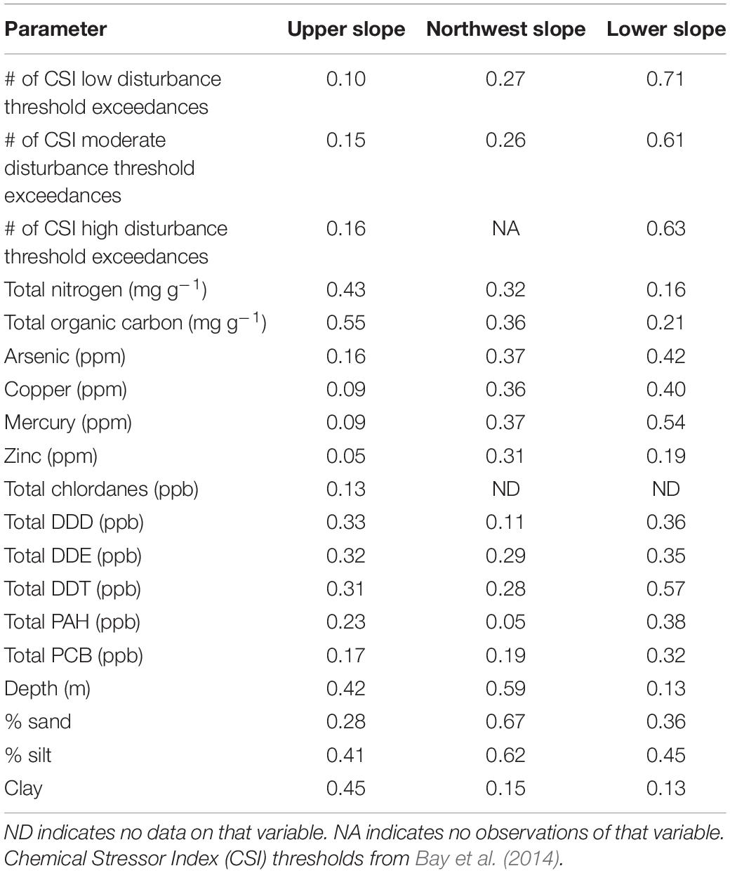
Table 2. Permutation-based correlations of stressors and natural environmental variables to ordinations of macrobenthic infauna at reference and non-reference samples in each of the three continental slope habitats (obtained from envfit function in R).

Within each habitat, the assemblage-scale relationship of reference and non-reference infauna samples was evaluated with non-metric multi-dimensional scaling (nMDS) ordinations based upon untransformed species-level and above abundances. Permutation-based Analysis of Variance (PERMANOVA) (Anderson, 2001) was used to determine if there were significant (α = 0.1) differences between the biota of the reference and non-reference samples. It should be noted that the authors elected to use an α = 0.1 based upon their comfort with a 10% level of type I error. Lastly, the chemical, macronutrient, and natural environmental variables were correlated to the nMDS ordinations of each habitat’s samples. All of the multivariate analyses were conducted with the Vegan package v2.4-4 in R (Oksanen et al., 2017) using the metaMDS function for the ordinations, adonis2 for the PERMANOVAs (untransformed abundance Bray–Curtis dissimilarities over 1,000 permutations), and envfit for the multivariate correlations.

Within each habitat, individual taxon abundance was correlated and plotted for visual inspection with each of the different chemical constituents as first step in identifying any potential taxa that could be useful for predicting contamination in other samples from their habitat. Any taxon-stressor relationships of note would subsequently be analyzed in a more rigorous fashion, using different modeling techniques (e.g., random forest, relative risk, and gradient forest). Given the rigorous sorting and identification procedures used to produce the benthic infauna data (e.g., County Sanitation Districts of Los Angeles County, 2016; City of San Diego, 2017; Gillett et al., 2017), absence of a taxon from a sample was treated as a “true absence” and assigned an abundance of 0 for all correlation analyses (Karenyi et al., 2018). Species richness (S) and Shannon–Wiener diversity (H′) values were also correlated to the different stressor measurements. All correlations were Spearman’s rank correlations and were calculated using the cor function in R.

The Influence of Time

The first step to understand the influence of time on the dataset and our analyses was to characterize basin-scale changes in community structure of the benthic fauna through time that were not related to local changes in the magnitude of anthropogenic disturbance (e.g., wastewater discharges and oil/gas extraction). Reference site benthic faunal data from each identified habitat were examined for changes in species identity and abundance, as well as the overall number of taxa across time frame of the study. Untransformed abundance data of taxa identified to the lowest possible taxonomic level were ordinated using non-metric multidimensional scaling (nMDS). Differences in the ordination space between decades was quantified using a 2-way PERMANOVA with decade of collection, habitat, and their interaction as the explanatory variables (α = 0.1). Post hoc, pairwise PERMANOVA comparisons of multivariate differences between habitats within a decade to evaluate the persistence of habitat distinctness through time were adjusted using a Holm correction (Holm, 1979). Taxa richness between decades within each habitat was evaluated using a Kruskal–Wallis test with Dunn post hoc tests using decade as the explanatory variable (α = 0.1).

The second step in understanding temporal influence on our analyses was to determine if any temporal patterns in the data influenced the relative differences between reference and non-reference samples within each habitat. Both reference and non-reference data benthic faunal data from each habitat were examined for changes in species identity and abundance between reference and non-reference samples within decade. The relative difference of the within-decade differences were then compared among each decade of sampling. Untransformed abundance data of taxa identified to the lowest possible taxonomic level were ordinated using non-metric multidimensional scaling (nMDS) (see Supplementary Material). Differences in the ordination space between condition status (reference/non-reference) and decades (1990, 2000, and 2010) were quantified using 2-way PERMANOVA with decade of collection, condition status, and their interaction as the explanatory variables (α = 0.1). Post hoc, pairwise comparisons of multivariate differences between reference and non-reference samples within a decade and habitat were adjusted using a Holm correction (Holm, 1979).

All of the multivariate analyses were conducted with the Vegan package v2.4-4 in R (Oksanen et al., 2017) using the metaMDS function for the ordinations and adonis2 for the PERMANOVAs (untransformed abundance Bray–Curtis dissimilarities over 1,000 permutations). Pairwise PERMANOVA comparisons were made with the pairwiseAdonis (v0.0.1) (Arbizu, 2017) and p.adjust functions in R. The Kruskal–Wallis tests were conducted using the kruskal.test function in R (v3.6.1).

Taxonomic vs. Geographic Similarity

Preliminary analysis of the infaunal data indicated a surprisingly small number of shared taxa among the different samples within a habitat compared to other parts in the region (Gillett et al., 2017). To quantify the lack of co-occurring taxa between samples, the similarity of the benthic infaunal samples were compared to each other in relation to their geographic proximity [i.e., distance decay of similarity (Nekola and White, 1999)]. Similarity was measured as Bray–Curtis dissimilarity between samples designated as reference within and between each slope habitat. Bray–Curtis values were calculated using taxonomic data at their lowest possible level of identification, but also at a taxonomically coarser operational taxonomic unit (OTU) level in an effort to create more homogenous taxa profiles (following Hawkins et al., 2000; Van Sickle et al., 2005) and therefore theoretically more similar samples. The OTUs were defined by first retaining all taxa (species or otherwise) occurring in more than 25 samples within each habitat’s reference samples. The remaining taxa were then collapsed to the genus level and those genera that occurred in more than 25 samples within each habitat’s reference samples were retained. All other taxa were discarded. Bray–Curtis values were calculated using vegdist function in the Vegan Package 2.4-4 from R and linear distance between samples was calculated from latitude and longitude using the geosphere package in R.

Results

Habitat Identification

The screening criteria classified 208 samples from 189 sites as reference out of the 750 (27%) total samples. Reference samples spanned the full depth (200–1,023 m) and geographic range (32.51629° N – 34.363147° N in latitude and −120.55833° W to −117.2805°W in longitude) of our dataset (Figure 1), with a temporal range of 1991–2016. The clustering routine of Bray–Curtis dissimilarity values yielded 5 different clusters of taxa (Supplementary Material 1). When placed in an nMDS ordination for easy visualization, samples from clusters 1, 2, and 3 contained the majority of samples and were relatively distinct from each other (Figure 2). Clusters 4 and 5 were very low-density clusters consisting of 6 samples (three in each). These six samples were lumped together with the samples from cluster 3 because of their proximity to cluster 3 in the ordination, their depth (>450 m), and their geographic location.

FIGURE 2

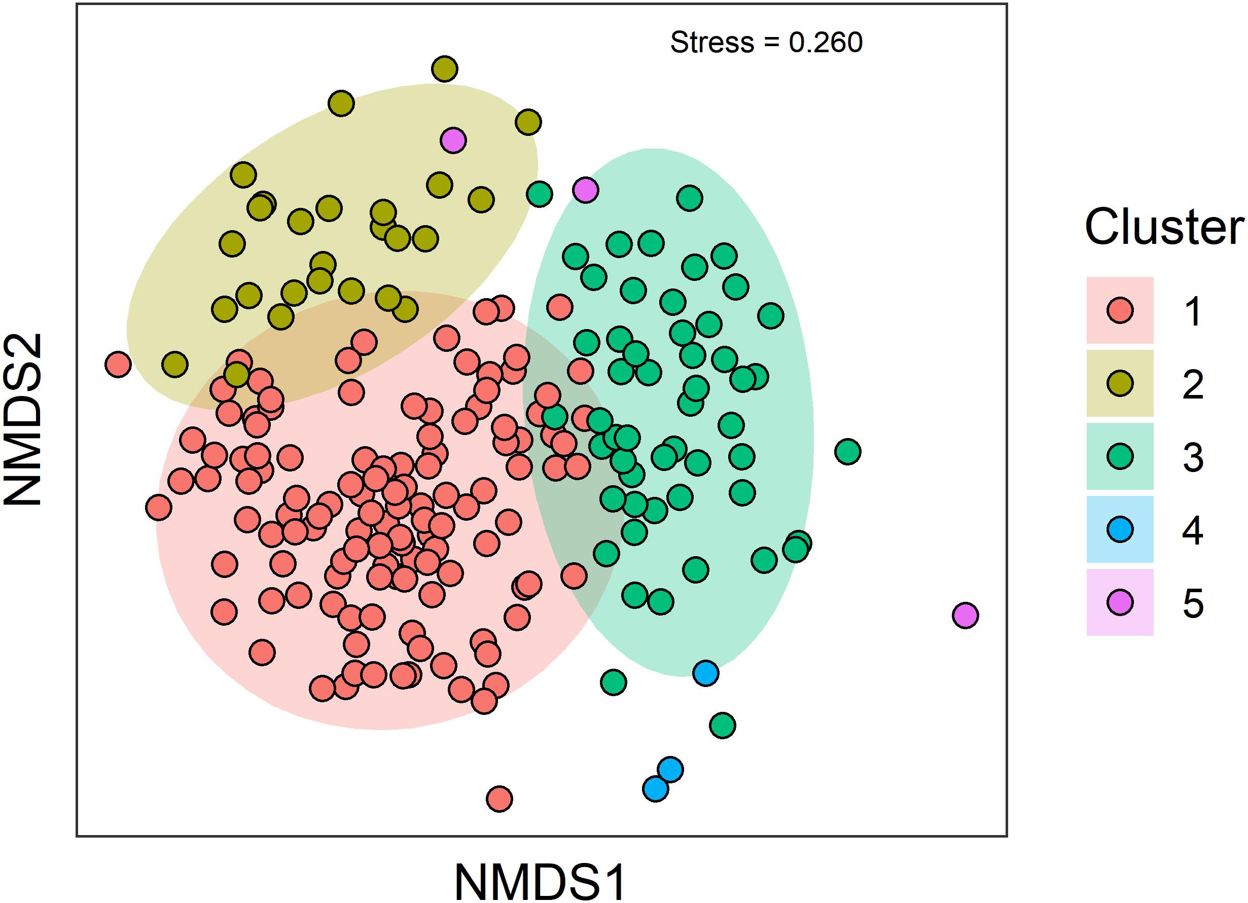
Figure 2. Two-dimensional plot summarizing the nMDS ordination of reference sites. Colors correspond to cluster membership of samples based upon Bray–Curtis dissimilarity of benthic fauna aggregated to the genus level. Ellipses represent multivariate-t distribution of cluster groups and are provided only as a visual guide of sample grouping.

The dominant taxa of each cluster (i.e., >1% of total abundance) were relatively different from each other (Supplementary Material 2), though there was a small amount of overlap between clusters 2 and 3 (plus 4 and 5). The maldanid polychaete Maldane sarsi was the only dominant taxon found in each habitat. From the community perspective, Cluster 1 had significantly greater species richness (Kruskal–Wallis Chisq = 83.98 df = 2,202 p < 0.001) and diversity (Kruskal–Wallis Chisq = 56.85 df = 2,202, p < 0.001) than cluster 3 (plus 4 and 5), which in turn was greater than cluster 2 (Figure 3).

FIGURE 3

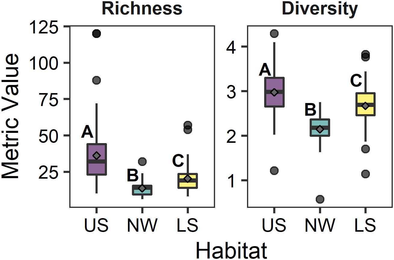
Figure 3. Schematic box-plots of species richness (S) and Shannon–Wiener Diversity (H′) among reference sites in each of the three deep water habitats. Gray diamonds indicate the mean value within each habitat (US, upper slope; NW, northwest slope; LS, lower slope). Letters indicate significantly (α = 0.1) similar/different habitats based upon Dunn post hoc comparisons of Kruskal–Wallis tests for each parameter between habitats. Boxes represent the 25th and 75th percentiles of each measurement, with the midline depicting the median value. Whiskers represent ±1.75× the interquartile range, with the dots depicting outlier values beyond the whisker.

As a whole, the samples of cluster 1 were shallower than those of cluster 2 or 3 (plus 4 and 5) (Kruskal–Wallis Chisq = 128.7, df = 2,202, p < 0.001). The sediments from cluster 1 contained a greater amount of sand (Kruskal–Wallis Chisq = 36.7, df = 2,202, p < 0.001), a lesser amount of silt (Kruskal–Wallis Chisq = 63.6, df = 2,202, p < 0.001), and similar amounts of clay (Kruskal–Wallis Chisq = 1.8, df = 2,202, p = 0.32) than the samples from the other clusters (Figure 4). All of the samples had sediments that could be classified as sandy-silt, with the sediments of cluster 1 being generally sandier than the other clusters, but still dominantly silt. The samples of clusters 2 and 3 (plus 4 and 5) were similar to each other with respect to sediment composition. The samples of cluster 3(plus 4and 5) were deeper than 2, which were deeper than cluster 1. When plotted on a map of the region (Figure 1), it became apparent that samples from clusters 1 and 3 (plus 4 and 5) were separated from each other along a depth break of approximately 400 m running the length of the region’s coastline until near Santa Barbara, CA, United States (∼−119.76911 longitude). Westward from there (∼−120.4562 longitude), across the full depth range, were the samples of cluster 2.

FIGURE 4

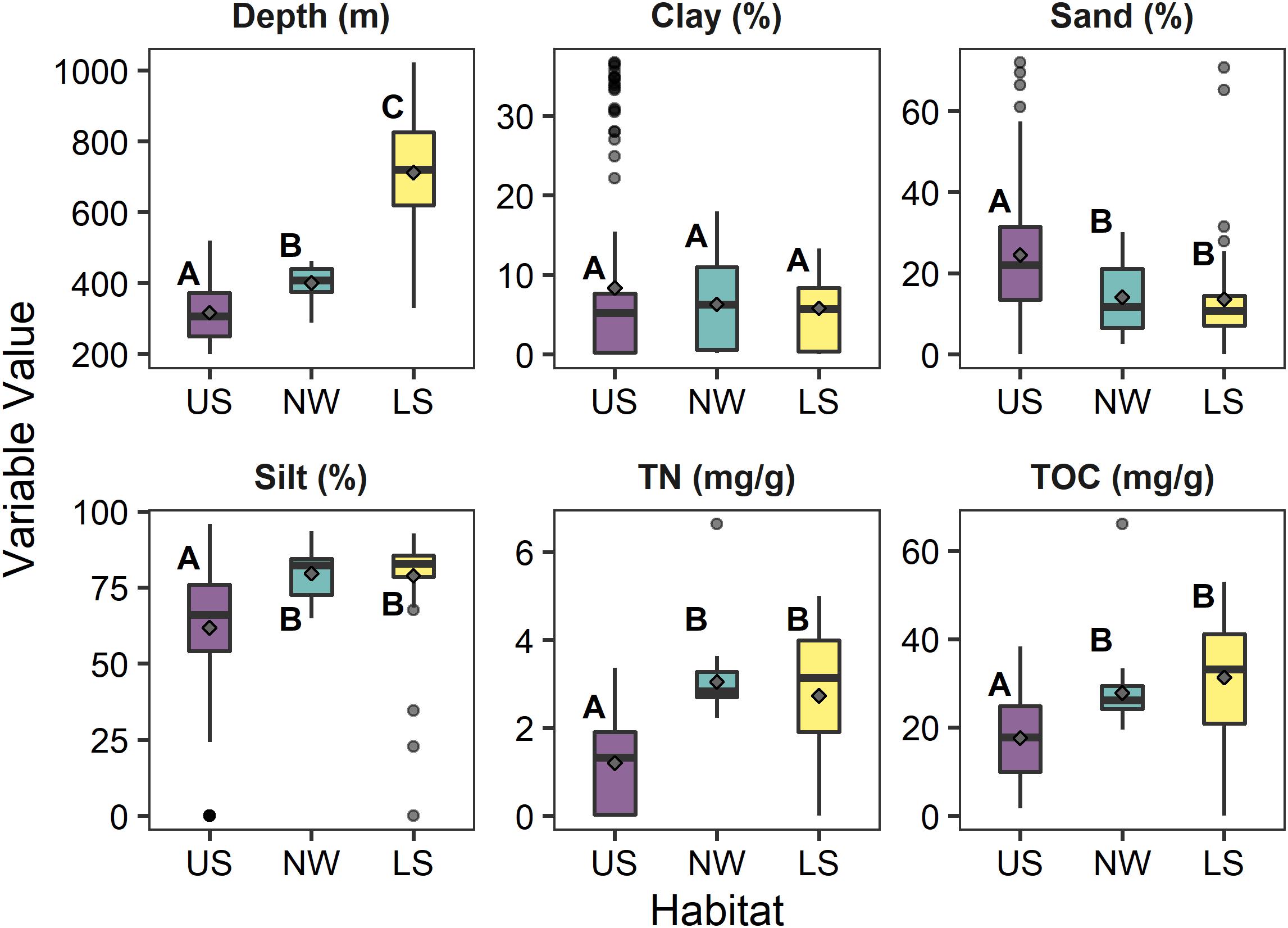
Figure 4. Schematic box-plots of depth (m), clay (%), sand (%), silt (%) total Nitrogen (TN mg g^{– 1}) and total organic Carbon (TOC mg g^{– 1}) among reference samples in each of the three deep water habitats (US, upper slope; NW, northwest slope; LS, lower slope). Gray diamonds indicate the mean value within each habitat. Letters indicate significantly (α = 0.1) similar/different habitats based upon Dunn post hoc comparisons of Kruskal–Wallis tests for each parameter between habitats. Boxes represent the 25th and 75th percentiles of each measurement, with the midline depicting the median value. Whiskers represent ±1.75× the interquartile range, with the dots depicting outlier values beyond the whisker.

Based on the biotic (Figure 2), abiotic (Figure 4), and geographic (Figure 1) differences among the reference samples, we have erected 3 habitats for the southern California continental slope:

• Habitat 1 (cluster 1) – The Upper Slope represents the shallow (∼200 – 400 m) shelf/slope transition habitat along the length of the coastline from Santa Barbara, CA, United States to Tijuana, Mexico. These sites cover a mix of sediment types from silty-sand to sandy-silt and have relatively low TOC and TN content.

• Habitat 2 (cluster 2) – The Northwest Slope represents sites between Santa Barbara, CA, United States and Point Conception, CA that covers a range of depth, a mix of sediment types, and a range of TOC/TN levels.

• Habitat 3 (clusters 3, 4, and 5) – The Lower Slope represents the deep-water (∼400–1,000 m) slope habitat along the length of the coastline from Santa Barbara, CA, United States to Tijuana, Mexico. These sites cover a mix of sediment types from sandy-silt to silty-silt and have elevated TOC and TN compared to the Upper Slope.

Disturbance Response

As illustrated in Figure 5, there were some strong correlations among abiotic variables as would be expected (e.g., strong direct correlation among the three CSI metrics, or a strong inverse correlation between % sand and total Nitrogen). However, none of these strong correlations represented major confounding factors (e.g., a theoretical strong relationship between depth and Copper), so any subsequent inferences drawn from the habitat-stressor-faunal relationships could be assumed to be relatively independent and more cleanly interpreted.

FIGURE 5

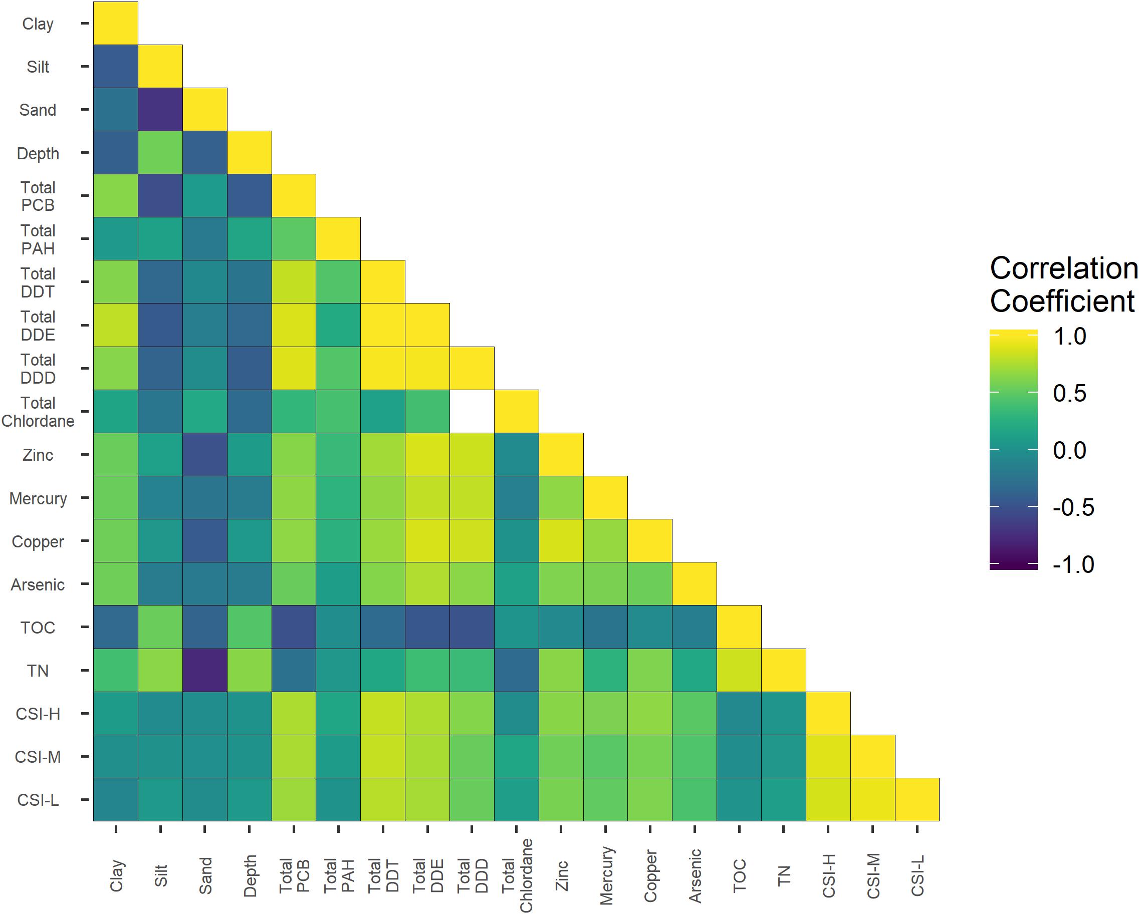
Figure 5. A heatmap depicting the relative correlation between the different potential stressors used in the study. Spearman’s correlation coefficients (r_s) were used, with yellow representing a strong direct correlation and purple representing strong inverse correlation. CSI-H, number of CSI high Impact threshold exceedances; CSI, M, number of CSI Moderate Impact threshold exceedances; and CSI-L, CSI low impact threshold exceedances. CSI thresholds after Bay et al. (2014).

From the multivariate perspective, visual inspection of the nMDS ordination plots for the Upper Slope and Lower Slope habitats (Figure 6) indicates that the fauna of reference and non-reference samples were not clearly distinct from each other. The pattern, however, suggests a gradient in composition from reference to disturbed samples within the same habitat. The visual pattern was confirmed by the PERMANOVA testing for differences between the reference and non-reference samples in the Upper Slope (PERMANOVA pseudo-F = 19.56, df = 1,562, p = 0.0012) and the Lower Slope (PERMANOVA pseudo-F = 5.49, df = 1,114, p = 0.0012) habitats. These two pieces of evidence indicate that the macrobenthic communities in the Upper and Lower slope habitats do experience compositional changes when exposed to disturbance. In contrast, both visual and statistical evidence indicated that there were no differences between the reference and non-reference samples in the Northwest Slope habitat (PERMANOVA, pseudo-F = 1.17, df = 1,30, p = 0.2035). The lack of a pattern, compared to the other deep-water habitats, may have been an artifact related to the small number of samples, of which only 5 were considered non-reference.

FIGURE 6

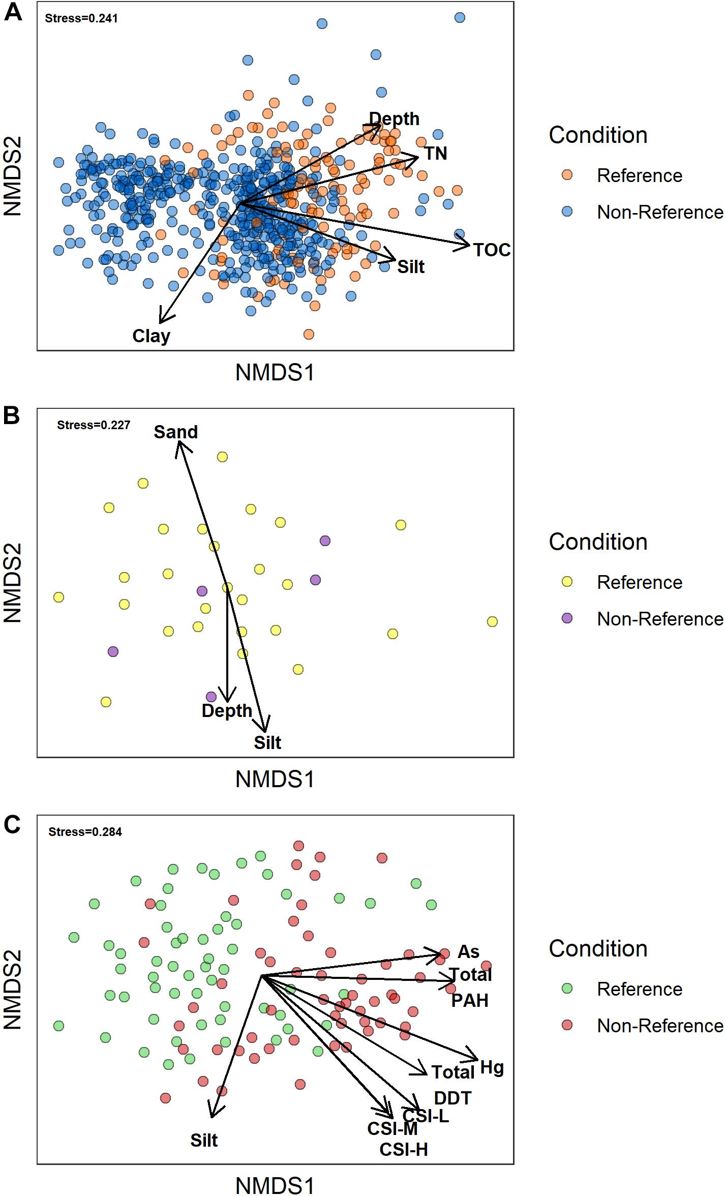
Figure 6. Two-dimensional plots summarizing the nMDS ordination of samples from: (A) upper slope, (B) northwest, and (C) lower slope illustrating the relative separation of reference samples from non-reference samples. The arrows represent vectors of influence for the different stressors and natural factors from Table 3 that had a permutation correlation coefficient greater than 0.4 [derived via the envfit function in vegan (Oksanen et al., 2017)] with the ordination as plotted. The length of the arrow is proportional to the magnitude of the correlation. CSI-H, number of CSI high impact threshold exceedances; CSI – M, number of CSI moderate impact threshold exceedances; and CSI-L, CSI low impact threshold exceedances. CSI thresholds after Bay et al. (2014).

The abiotic variables from Table 2 that had a multivariate correlation coefficient greater than 0.4 with the ordination patterns are plotted as vectors in Figure 6. Though nearly all of the correlations were statistically significant (α = 0.1) to the ordination of the Upper Slope habitat, only TN and TOC had non-spurious relationships (i.e., r > 0.4) with the ordination, as did water depth, % silts, and % clays. Sediments from reference sites had greater amounts of TN than non-reference sites, which also seemed to co-occur with deeper samples within the habitat. Based on the direction of their vectors, silt and TOC content of the sediments appear to explain some of the differences in samples within the reference and non-reference groups of the Upper Slope, but not between the reference and non-reference samples from the other two habitats.

In the Lower Slope habitat, fewer stressors were significantly (α = 0.1) correlated to the ordination than in the Upper Slope habitat (Table 2). This pattern was most likely driven by sparser density of stressor data in the Lower Slope compared to the Upper. However, of those stressors that were not spuriously related to the ordination, Mercury, Arsenic, total PAH, and total DDT concentration, as well as all three levels of CSI threshold exceedance, were higher in the non-reference samples compared to the reference samples. This pattern would suggest that these toxic chemicals were, in part, responsible for the differences in community composition between the reference and non-reference samples.

From the univariate perspective, Spearman’s rank correlations of species richness (S) and Shannon–Weiner species diversity (H′) with the stressors from Table 2 were calculated within each habitat and across all deep-water habitats (Table 3). Species diversity in the Upper Slope was inversely related (r_s < −0.47) to concentrations of Copper, Zinc, total DDD, and total DDE. As concentrations of these chemicals increased, species diversity declined. There were no such similar patterns in either the Northwest or Lower slope habitats.

TABLE 3

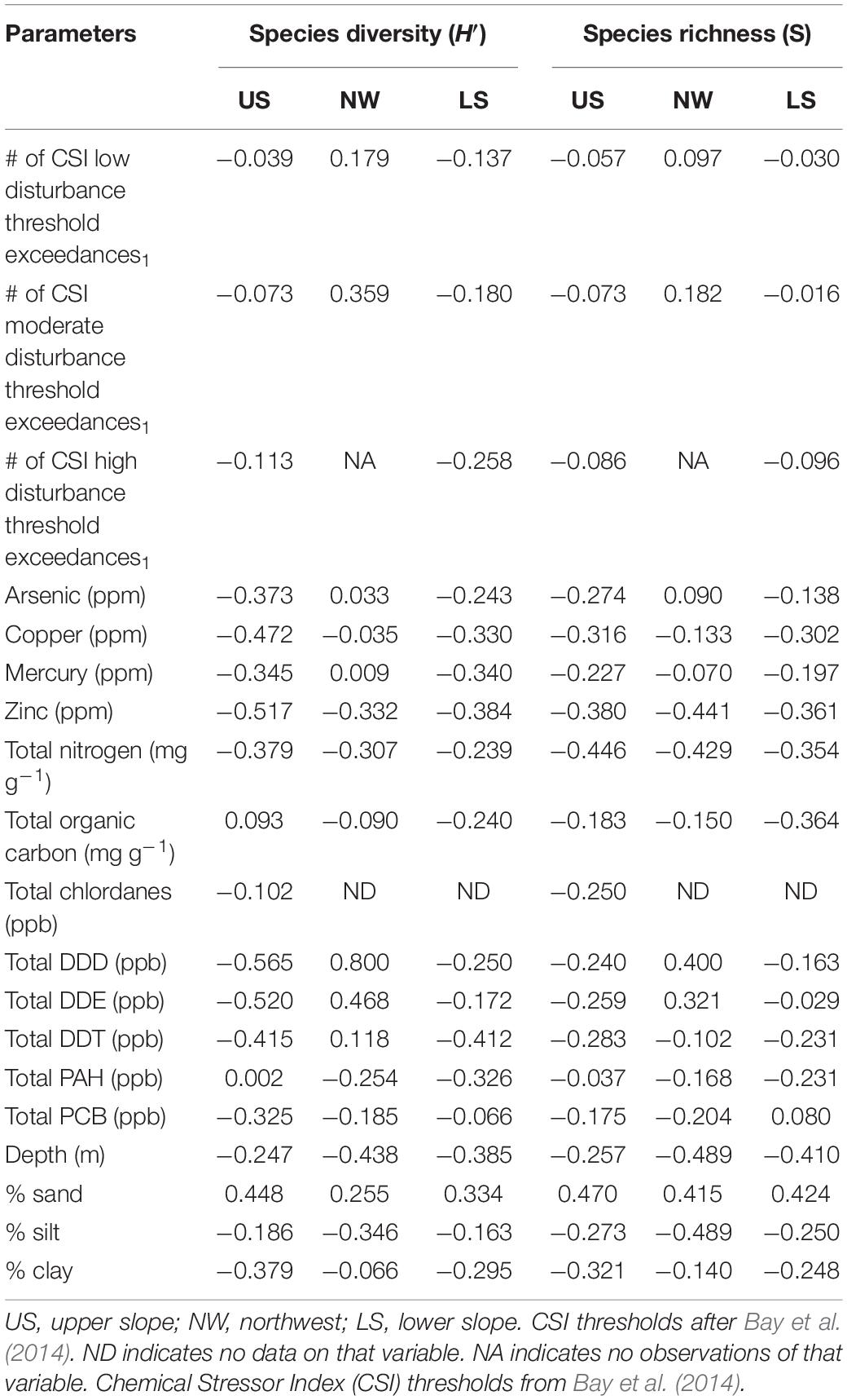
Table 3. Spearman’s rank correlation coefficients for macrobenthic infauna Shannon–Weiner Diversity or species richness with the stressors and natural environmental variables in each of the continental slope habitats.

Of the 1,011 taxa from the Upper Slope and the 527 from the Lower Slope, there were less than 20 Spearman’s ranked correlations with the 15 different stressors listed in Table 2 that had r_s values >0.4 or <−0.4. The lack of any meaningful patterns among the 18,660 potential taxon-stressor combinations was mostly likely due to no single taxon being frequently observed across the samples of a given habitat, combined with a lack of consistent chemical detections in the same samples where a taxon was observed. Nearly all of the taxa observations in Upper and Lower slope habitats were dominated by zero-counts. As such, the identification of any individual taxon-stressor relationships in a simple correlation framework was not successful.

Temporal Influence

Visual inspection of the nMDS ordinations of the fauna observed at reference condition sites from each the three habitats indicates that there were changes in each habitat through time (Figure 7). However, the lack of discrete groupings by decade would suggest that the changes were gradual shifts in the peripheral taxa, not wholesale replacement of the community dominants. The change in fauna across the decades within each habitat was confirmed by the results of the overall PERMANOVA, where decade was a significant factor in the taxonomic composition within each habitat (Upper Slope – d.f.: 2,115, Pseudo-F = 3.27, p < 0.001; Northwest Slope d.f.: 1, 25, Pseudo-F = 1.61, p = 0.006; Lower Slope d.f.: 1,61, Pseudo-F = 2.54, p < 0.001).

FIGURE 7

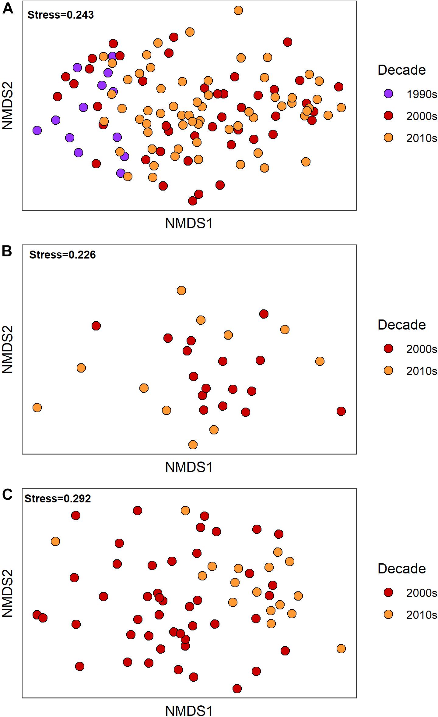
Figure 7. Two-dimensional plots summarizing the nMDS ordinations of reference samples (untransformed benthic infauna abundance) from (A) upper slope, (B) northwest, and (C) lower slope continental slope habitats. The color of the dots indicates the decade during which the samples were collected.

Habitat distinctness through time was evaluated by comparing the fauna of reference sites from each habitat within different decades (Table 4). However, within decade comparisons of habitat distinctness could only be made for data from the 2000s and 2010s, as no reference samples were available for the Northwest and Lower slope habitats from the 1990s. The 2-way PERMANOVA with decade and habitat as factors indicated that the fauna of the three habitats were significantly different from each other in the 2000s and 2010s (Table 4).

TABLE 4

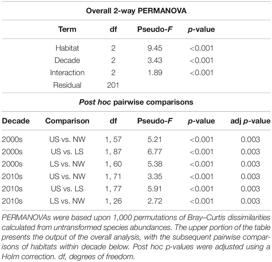
Table 4. Two-way PERMANOVA results comparing macrobenthic community composition of reference samples among habitats Upper Slope (US), Northwest Slope (NWS), and Lower Slope (LS) – and among a decade of sampling – 1990s, 2000s, and 2010s.

Among the reference samples from the three habitats, there were no differences in taxa richness between decades in the Upper Slope (Kruskal–Wallis Chisq = 0.153, d.f. = 2, 115, p = 0.926) and Northwest Slope (Kruskal–Wallis Chisq = 0.841, d.f. = 1, 25, p = 0.359). In contrast, there was greater taxa richness among the lower slope samples from the 2010s compared to the 2000s (Kruskal–Wallis Chisq = 6.59, d.f. = 1, 61, p = 0.01) (Figure 8).

FIGURE 8

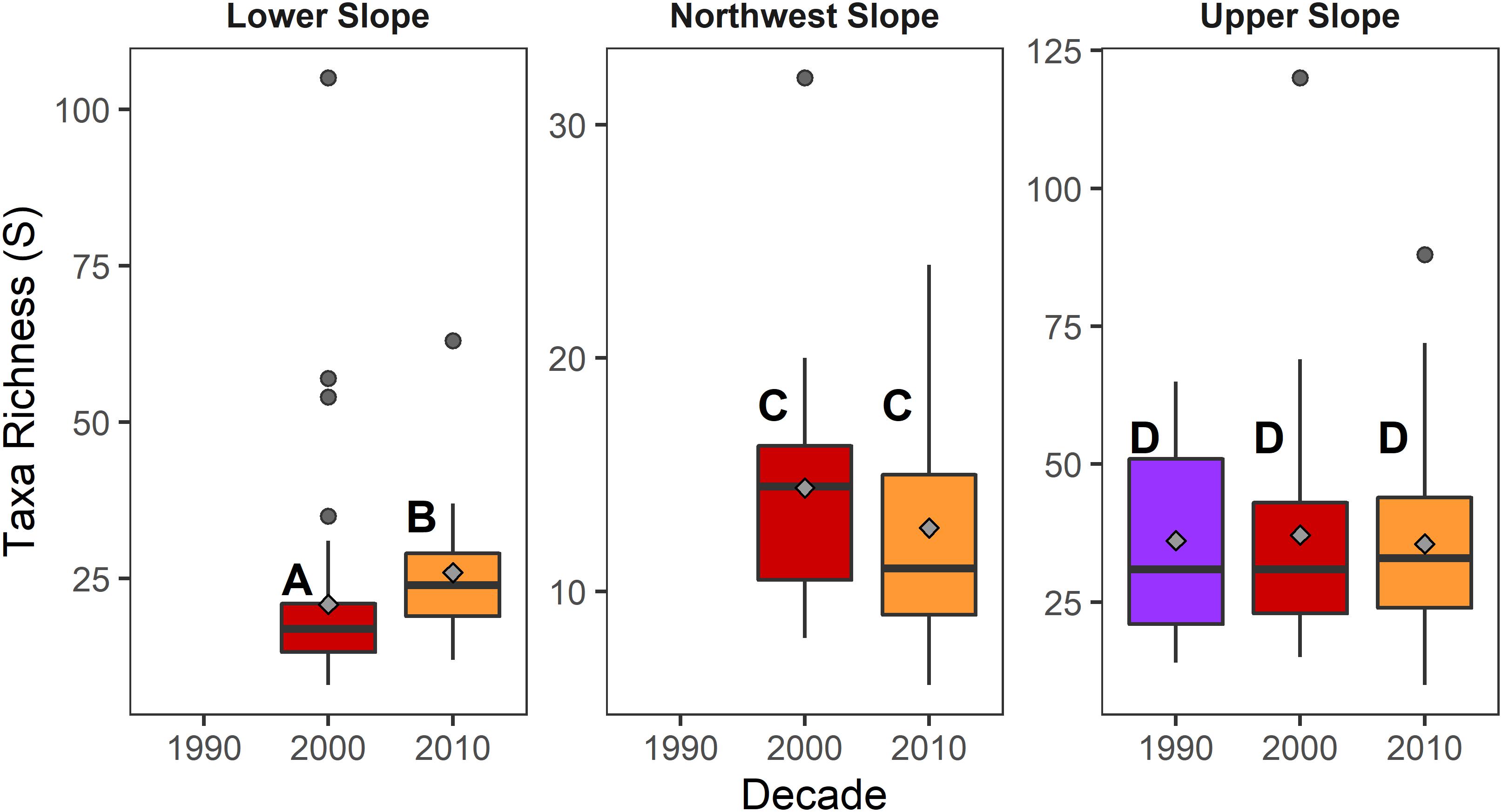
Figure 8. Schematic box plots of taxa richness among reference samples collected in different decades from each of the three continental slope habitats. Gray diamonds indicate the mean value within each decade-habitat combination. Letters indicate significantly (α = 0.1) similar/different decades based upon Dunn post hoc comparisons of Kruskal–Wallis tests for each parameter between decades within a given habitat. Boxes represent the 25th and 75th percentiles of each measurement, with the midline depicting the median value. Whiskers represent ±1.75× the interquartile range, with the dots depicting outlier values beyond the whisker.

The results of the PERMANOVA comparing reference and non-reference samples with decade and reference status as factors by habitat indicated significant temporal changes in the fauna in both types of samples within each habitat (Table 5). As noted earlier, no reference samples were available among the 1970s and 1980s Upper Slope data. Similarly, no samples of any condition were available for either the Lower or Northwest slope habitats prior to the 2000s. The significant differences in faunal composition observed between reference and non-reference samples in the combined dataset (Figure 6) persisted when the individual decades were considered in isolation: 1990s, 2000s, and 2010s for the Upper Slope; and 2000s and 2010s for the Lower Slope. Interestingly, the PERMANOVA of the Northwest Slope data from the 2000s (Table 5) indicated a significant difference in composition of the reference and non-references samples. This differs from the analysis of the combined dataset for the Northwest Slope, which indicated no significant differences in composition between reference and non-reference samples. See Supplementary Material 3 for visual illustrations of the nMDS ordinations between reference and non-reference samples in each habitat and decade.

TABLE 5

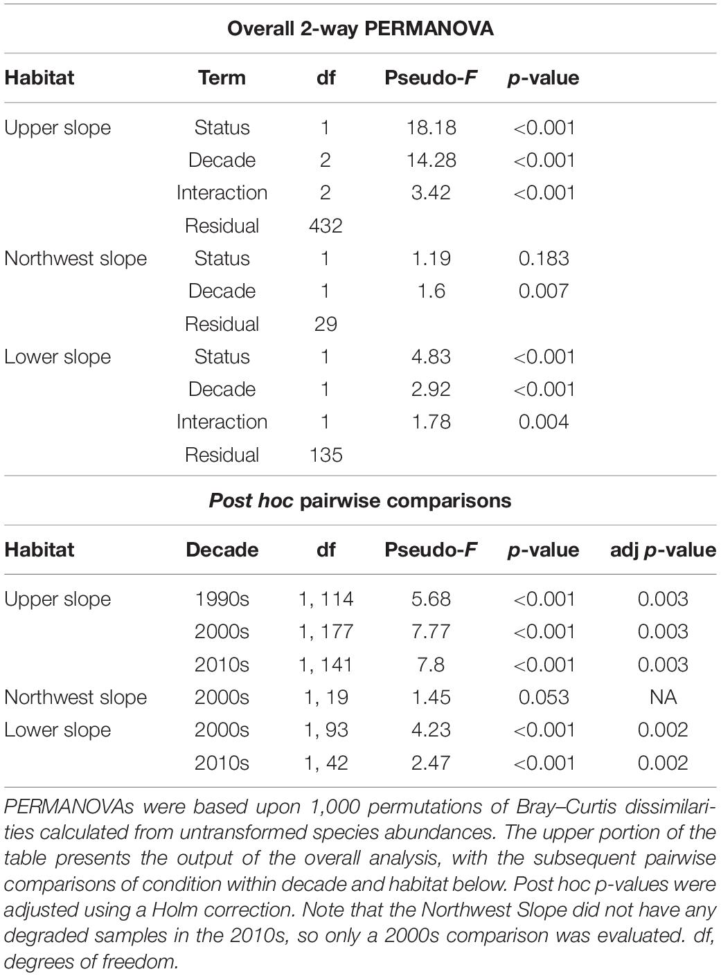
Table 5. Two-way PERMANOVA results comparing macrobenthic community composition of reference and non-reference samples among habitats – Upper Slope, Northwest Slope, and Lower Slope – and among decades of sampling – 1990s, 2000s, and 2010s.

Taxonomic and Geographic Similarity

As illustrated in Figure 9, reference samples within each habitat that were spatially close to each other (≤1 km) were quite compositionally different from each other (e.g., Bray–Curtis dissimilarity >0.5). Table 6 illustrates that, on average, any reference sample from one habitat was as dissimilar to another reference sample from its habitat as those from a different habitat. When sample-to-sample comparisons were made with OTUs, the overall dissimilarity was smaller, but the mean dissimilarity was still nearly as great within habitat as between habitats.

FIGURE 9

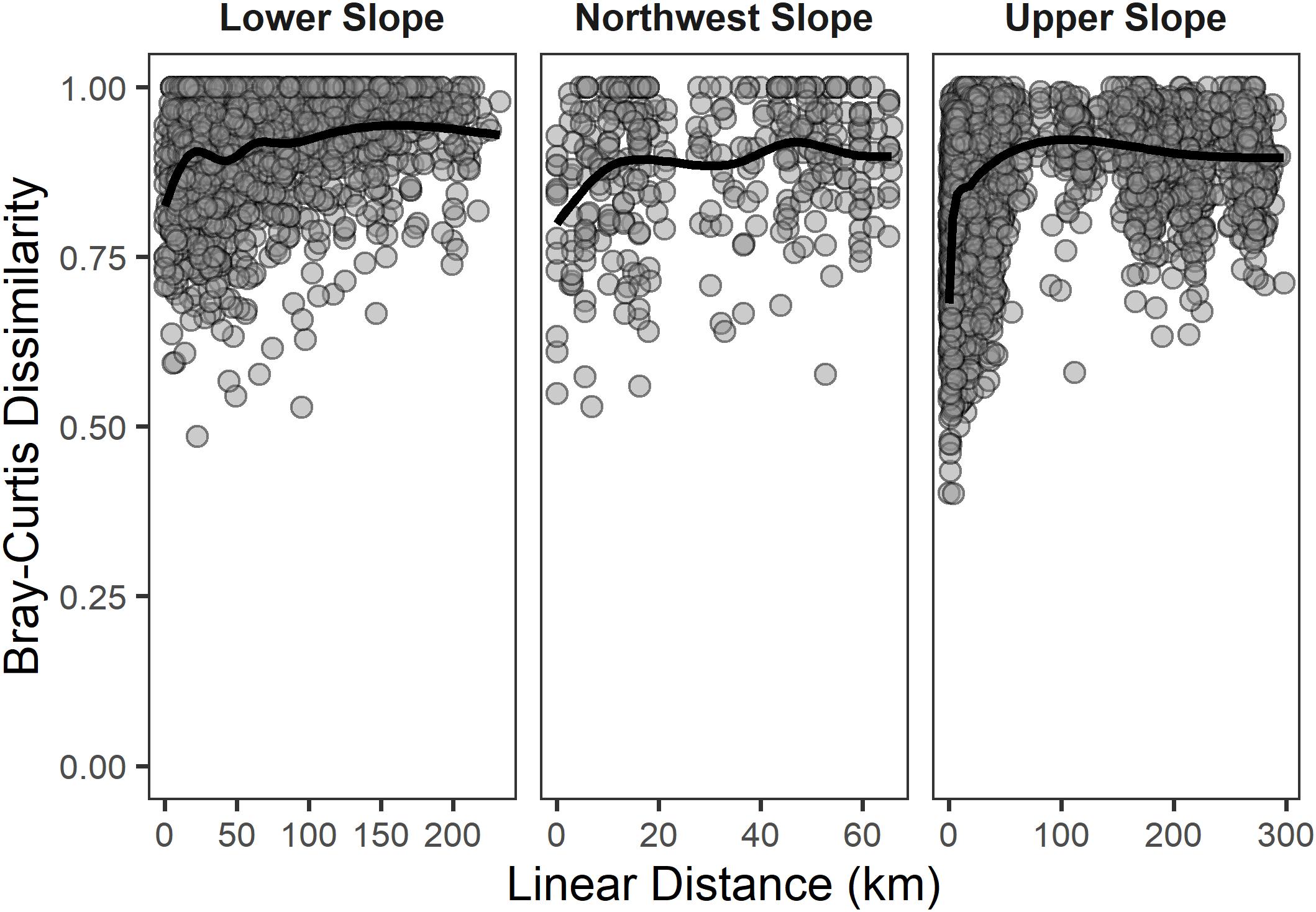
Figure 9. Scatter plots of pair-wise Bray–Curtis dissimilarity of reference samples from each continental slope habitat plotted against the pair-wise linear distance between the samples. Dissimilarities were calculated using non-transformed abundance of taxa at the lowest possible taxonomic level. The black line depicts a general additive model smoothed mean to aid in visualization of the pattern given the density of points and the subsequent over-plotting of data points.

TABLE 6

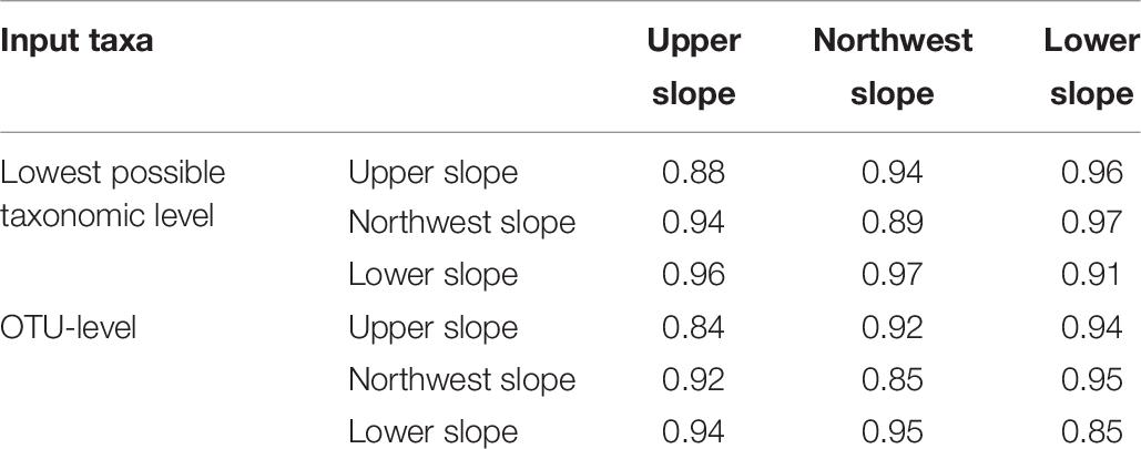
Table 6. Mean pair-wise Bray–Curtis dissimilarity values calculated from non-transformed abundance between reference samples in each of the three habitats of the continental slope ecosystem using the lowest possible level of taxonomic resolution, as well as Operational Taxonomic Unit -level taxonomic resolution.

Discussion

This work represents the most comprehensive study of regional ecological patterns in the benthic infauna of the southern California continental slope ecosystem since the Allan Hancock cruises of the late 1950s (Hartman, 1955, 1966; Hartman and Barnard, 1958, 1960). The present work covered broader temporal and spatial scales than the Hancock cruises did, with a more complete distribution of samples across the depth gradient from the continental shelf down to the upper portions of the continental slope. This scale makes the present study relatively unique for a benthic study at these depths. Furthermore, that scale that was only made possible because the bulk of these data were the product of a collaborative, regional monitoring partnership [Southern California Bight Regional Monitoring Program (Schiff et al., 2016)] that enables consistency in taxonomy, data collection and data quality standards across multiple decades of surveys.

Our analysis of benthic infauna survey data identified three relatively distinct natural biological communities that are characteristic of different habitats across the continental slope of the Southern California Bight. The primary segregating feature between the two largest habitats was depth, with separation at approximately 400m depth. Water depth and the attendant exposure of fauna to different water masses with their own temperature regimes, oxygen dynamics and hydrostatic pressures are an important barrier in the biogeography of seemingly contiguous deep sea benthic habitats (e.g., Rex, 1981; Hyland et al., 1991; Levin et al., 1991; Rex et al., 2005). Across the California Current, the depth of the oxygen minimum zone will vary with latitude (Helly and Levin, 2004). In the southern portions of the California Current system, 400 m has been reported as the approximate boundary between the oxygen limited (O₂ between 0.7 and 2.1 mg L^–1) and oxygen minimal (O₂ < 0.7 mg L^–1) zones (Bograd et al., 2008; Gilly et al., 2013). These dissolved oxygen dynamics likely contribute in part to the differences in benthic community composition observed between the Upper and Lower slope habitats.

Beyond the depth-related separation of habitats, there were some quantitative differences in sediment composition that paralleled the depth differences between the Upper and Lower slope habitats. There was a general trend of silt content of sediments increasing with depth, as did the TOC and TN content of those sediments. This pattern is similar to those observed in other upwelling dominated systems, where the currents and nutrient dynamics increase the production of biogenic material and low oxygen conditions slow its degradation in the sediment (Calvert et al., 1995; Sifeddine et al., 2008; Arndt et al., 2013). However, the sediments of both habitats would be considered silty muds from a benthic faunal perspective and unlikely to contribute substantially to the differences in community composition observed between the two habitats (though see Henkel and Politano, 2017).

After water depth, the secondary segregation between habitats was geographic. The third habitat was centered on the most northwestern portion of the Southern California Bight, west of Santa Barbara, CA, United States, and spanning both sides of depth-related break in community composition separating the Upper and Lower slope habitats elsewhere in the region. This portion of the Southern California Bight is a biogeographic break-point, transitioning from cold-water fauna of central and northern California to the warm-water fauna of the south (e.g., Hyland et al., 1991; Bergen et al., 2001; Bergen, 2006; Henkel and Nelson, 2018). The fauna of the Northwest habitat were a mix of those from our Lower Slope habitat and those from further north along the California coast (see Hyland et al., 1991). Oceanographically, this is also a unique portion of the region. There is an eddy system in the Santa Barbara Channel that increases the exposure of the fauna to corrosive low-pH waters (Oey, 1996; Hauri et al., 2013; Turi et al., 2016) compared to the other habitats we identified.

Our identification of three relatively distinct habitats differed from the pattern previously described by Hartman and Barnard (1958, 1960), who described the deep basins as a relatively homogenous, relatively depauperate habitat. The difference may be due to Hartman and Barnard’s focus on the deepest parts of the region. All of their samples were from approximately 400 to 2,000 m (i.e., below our Upper Slope habitat), including a large number of samples west of the Channel Islands (i.e., west of our sampling area). The Lower Slope and Northwest Slope habitats of our study were closest to the area detailed by Hartman and Barnard, but even where the overlap was closest, at a maximum depth of 1,000 m we observed greater abundance and diversity of infauna than Hartman and Barnard (1960).

The results from our study indicated there has been some change in the composition, diversity, and density of deep-sea macrofauna of the Southern California Bight since the 1950s, as well as within the temporal scope of our sampling period. However, the unbalanced distribution of reference samples in the dataset and the confounding factor of condition/health of the Southern California Bight steadily improving since the 1970s limits the ability to fully characterize the temporal changes of the fauna and how those changes influence our findings. Within the time frame of our dataset, there were observable changes in the fauna among both reference and non-reference samples. Among the reference samples, differences in faunal composition across the years may be reflective of changes in basin-scale oceanographic factors like temperature, productivity, water chemistry or oxygen levels (e.g., Meinvielle and Johnson, 2013; Pozo Buil and Di Lorenzo, 2017; Breitburg et al., 2018; Bograd et al., 2019). These processes can influence both the survival of adults, as well as the larval disbursement and success of recruitment (e.g., Young and Eckelbarger, 1994; Levin and Gage, 1998; Ruhl and Smith, 2004). Among the non-reference samples, the changes in benthic community composition likely reflect basin-scale factors, as well as ongoing reductions/burial of anthropogenic contaminants in sediments since the 1970s (e.g., Smith et al., 2001; County Sanitation Districts of Los Angeles County, 2016).

Despite the changes in composition, the overall communities of the reference samples in each habitat remained distinct from each other across the decades. The persistence of the distinct communities supports the notion that the three habitats are a reasonable and ecologically meaningful perspective with which to consider the continental slope benthos of the region. Furthermore, there was a persistence of differences in faunal composition between reference and non-reference samples through the decades, where the comparison could be made. The persistence of distinct degraded and non-degraded communities supports the notion that there are detectable, community-scale effects of disturbance in these systems that could be used in developing condition assessment tools. However, assuming that baseline, reference condition benthic communities will continue to change through time as has been observed in the present dataset, reference definitions and the taxa profiles of reference condition locations should be periodically revisited in the future, especially once assessment tools are developed.

One of the key benefits to studying patterns in benthic community composition is the insight it typically provides into anthropogenic disturbances. Within the Upper and Lower slope habitats, we were able to detect indications of community-scale change across and within the decades characterized in both univariate and multivariate contexts that were associated with exposure to toxic chemicals and greater amounts of organic matter. However, none of these patterns were strong enough to be useful in providing a biological measure of disturbance. Furthermore, there were no discernable stressor-response patterns among the individual taxa that comprised these communities.

There are a variety of different anthropogenic and natural stressors that can influence the structure of benthic communities (e.g., Lenihan et al., 2003; Breitburg and Riedel, 2005; Gunderson et al., 2016). Though there are myriad of individual potential stressors in the environment, it is reasonable to group them into major classes of toxic chemicals, eutrophication, habitat alteration, physical disturbance, and altered water quality (e.g., elevated temperature, hypoxia, and acidification). In the present study, we were able to reasonably characterize potential exposure to toxic chemicals and eutrophication (i.e., Tables 2, 3), and the conclusions we can draw from these data are most likely sound. However, we were unable to fully characterize stress from physical disturbance (e.g., bottom trawling or mineral extraction) due to incompatible spatial resolution (United States Geological Survey, 2016) or altered water quality (e.g., low dissolved oxygen, low pH, or altered temperature). Exposure to low dissolved oxygen and acidification are important factors that may alter benthic community structure (e.g., Levin et al., 2001; Ruhl and Smith, 2004; Widdicombe and Spicer, 2008; Sato et al., 2017) that we could also not directly account for. As such, it is possible that the differences in reference and non-reference communities observed in the upper and lower slope habitat could be related to these or other uncharacterized stressors; none of which would be detected in our sediment chemistry focused stressor-response analyses.

It should also be noted, that the lack of detectable stressor-response patterns among individual taxa was at least in part due to the relatively low frequency of occurrence among any one taxon. Of the 1,011 taxa observed in the Upper Slope habitat, only 9 occurred in more than 50% of the samples and 941 taxa occurred in less than 10% of the samples. Similar patterns were observed in the Lower Slope (no taxon found in more than 50% of the samples) and Northwest habitats (only 1 taxon in more than 50% of the samples).

Patterns in species richness and alpha diversity reported from other continental slope and deeper environments around the world are not dissimilar to those observed in the present study (e.g., Blake and Grassle, 1994; Rex et al., 2000; Schaff et al., 2000). However, none of these studies had the geographic scale combined with high data density of our work to allow for comparable measures of beta diversity to be made. The pattern of taxa dispersion we observed – high beta diversity, but apparently little overlap in shared taxa from sample to sample – was surprising. It is reasonable to expect greater taxonomic dissimilarity in a non-disturbed location versus a disturbed one (e.g., Levin et al., 2000; Saracho-Bottero et al., 2020), but the heterogeneity observed in the present study was beyond that. Furthermore, this is quite a different pattern than observed among the macrobenthic communities of the shallower continental shelf and coastal embayments of southern California (Gillett et al., 2017) and other regions (e.g., Ellingsen, 2001, 2002).

High beta-diversity within a habitat, as well as between spatially adjacent habitats, despite coming from a physically homogenous setting, is suggestive of a community that is not organized by species-specific niches (sensu Hutchinson, 1959). These patterns instead are suggestive that the macrobenthic infauna of the Southern California Bight continental slope could fall under the concept of a neutrally organized community (e.g., Hubbell, 2001, 2005; Leibold and McPeek, 2006). Neutral community theory posits that the faunal abundance a location can support is relatively stable and constrained (i.e., a carrying capacity of a set number of individuals). As individuals die, they are not directly replaced by con-specifics optimized for the open niche space, but rather new recruits settle randomly from any taxon in the regional larval pool at that moment (Ricklefs, 2006).

The temporal changes in the fauna among the reference samples in each habitat were detectable in the taxa identity and abundance (via the multivariate analyses). In contrast, the changes were not detectable in the overall taxa richness for the Upper and Northwest slope habitats. This pattern is suggestive that the mode of change in these habitats may be species replacement. However, in the Lower Slope there was an increase the number of taxa concurrent with the overall change in community composition. This pattern does not preclude species replacement, but clearly indicates an overall increase in total beta diversity, which fits with the notion that the Lower Slope habitat could be characterized as neutrally organized.

Condition Assessment of the Continental Slope

We do not know how a neutrally organized community would interact with the way habitat condition is traditionally assessed. Many of the assessment tools that are typically used [e.g., tolerance indices (Borja et al., 2000; Smith et al., 2001), species-specific Multi-Metric Indices (Weisberg et al., 1997; Hunt et al., 2001) or predicted assemblage indices (Hawkins et al., 2000; Ranasinghe et al., 2009)] are built upon species identity and the premise that there are core assemblages of species living in a location that predictably change under exposure to stress (see Diaz et al., 2004 for a detailed review of most types of assessment frameworks). In this paradigm, disturbance pushes a superior competitor out of a niche and a more tolerant, but less-efficient competitor is able to flourish in the superior competitor’s absence (e.g., Pearson and Rosenberg, 1978; Rhoads et al., 1978; Gray et al., 2002; Pawlowski et al., 2014). Inherent in this premise is that both types of competitors have a reasonable degree of fidelity to their habitat. It is assumed that under non-disturbed conditions, the adults or larvae of the weaker competitor are not absent from the system, but instead have a consistent, low-level background presence and can take advantage of disturbance/vacated niches space.

However, if the assemblage captured in a given sample is the product of stochastic recruitment and extirpation as suggested by Hubbell (2005), then the species-specific, successional views of macrobenthic response to stress – that rely on predictable shifts in dominance from species A to B to C – may not work as well. The challenge of doing bioassessment with a neutrally organized community would be how to balance the very large amounts of variance associated with species composition between samples with the variance that could be imparted to a sample from exposure to stress (e.g., Hawkins et al., 2010). From the technical perspective, this equates to the selection of an underlying assessment approach that is mathematically robust to zero-inflated/median -zero species distributions or that avoids reliance on species-level patterns.

One potential option for developing an assessment framework for the continental slope infauna would be to not focus on species-level measurements of community composition, which are highly variable in these habitats, but instead develop a tool that functions on non-taxonomic properties of a community. Assessment frameworks could be developed to compare the autecological traits of the fauna in samples (e.g., feeding guilds, living position, and natural history). This type of biological trait analysis, aggregating multiple species into a single, potentially less variable measure, could be used to infer habitat condition from changes in traits across a gradient of stressor exposure rather than individual taxonomic units (e.g., Feio and Dolédec, 2012; Oug et al., 2012; Leaper et al., 2014).

A second option would be, in lieu of trying to minimize species-specific variance, to express all of the variance for each species together in a multivariate fashion for each distinct habitat with reference sites. These multivariate data could be presented visually in ordination space (e.g., Figure 6) and thresholds or envelopes could be constructed around the reference sites and the position of a new sample with respect to that reference envelope in multivariate space could be used to quantify its condition (e.g., reference, non-reference, or indeterminant). Alternatively, a measure of dissimilarity between a new sample and that of the reference sites could be used to quantify the sample’s condition with a univariate measure that still takes all of the species in a sample into consideration (e.g., Van Sickle, 2008).

A third approach would be to develop a modified version of a traditional Observed:Expected (O/E) model that measures disturbance based upon the species observed in a sample compared to those predicted to occur in a location under reference conditions. Expectations are the product of species occupancy models informed by natural abiotic forcing factors (e.g., Hawkins et al., 2000; Mazor et al., 2016). However, with the low frequency of occurrences and high beta diversity of the continental slope infaunal community, these types of models (e.g., classification random forest, discriminant function analysis) could not discriminate samples in the present dataset (Gillett pers obs). However, if an O/E index could be built from predictive joint-species distribution models (e.g., Pollock et al., 2014; Clark et al., 2017) (models that can mathematically handle large amounts of species absences and zero inflated data) of reference communities for each of the continental slope habitats, then an O/E approach could still provide a viable solution to assessing condition.

Though none of the aforementioned scenarios have been tested in a real-world setting, there are clearly options to explore for the development of an assessment framework in the continental slope habitats of southern California. Creating new tools like those described above, or retrofitting existing local [e.g., BRI (Smith et al., 2001)] or generalized [e.g., AMBI (Borja et al., 2000)] assessment tools to work with a potentially neutrally organized response to disturbance are reasonable options to consider. Irrespective of which approach to condition assessment is investigated, the datasets assembled for the present study would serve as an excellent starting point. We have delineated three unique benthic habitats across the region and identified reference samples within each one. Sampling of additional potential stressors to the benthic fauna, such as bottom water oxygen, temperature, and carbonate chemistry, as well as sediment composition and contaminants, would also allow for the characterization of stressor-response relationships covered in the present study as well as other stressors we could not consider due to a lack of bottom water data. Furthermore, given the temporal changes observed in the benthic community in this study and the decadal shifts in oceanographic currents (e.g., Meinvielle and Johnson, 2013; Bograd et al., 2019) any future assessment tools should incorporate temporal flexibility in reference community composition and stressor exposure/interaction.

Data Availability Statement

The data generated for this study is subject to the following licenses/restrictions: the regional survey data are publicly available and the remaining data sets are available upon reasonable request. Regional survey data are available from https://www.sccwrp.org/about/research-areas/regional-monitoring/southern-california-bight-regional-monitoring-program/bightprogram-data-portal/. Requests for the other data sets should be coordinated with DG, davidg@sccwrp.org.

Author Contributions

DG was responsible for the conceptualization of the study, the data analysis, data visualization, writing, and editing. LG was responsible for acquisition of funding, conceptualizing the study, writing, and review. KS was responsible for conceptualization, editing, project administration, and supervision. All authors contributed to the article and approved the submitted version.

Funding

Study collaboration and funding were provided by the United States Department of the Interior, Bureau of Ocean Energy Management (BOEM), Environmental Studies Program, Washington, DC, under Agreement Number M16AC00013 between BOEM and the Southern California Coastal Water Research Project (SCCWRP). This work has been technically reviewed by BOEM, and it has been approved for publication. The views and conclusions contained in this document are those of the authors and should not be interpreted as representing the opinions or policies of the United States Government, nor does mention of trade names or commercial products constitute endorsement or recommendation for use.

Conflict of Interest

The authors declare that the research was conducted in the absence of any commercial or financial relationships that could be construed as a potential conflict of interest.

Acknowledgments

The authors thank Marcus Beck, Valerie Goodwin, and Abel Santana for help with data organization and help with some of the analyses. The authors also thank the Southern California Bight Regional Monitoring Program, Sanitation Districts of Los Angeles County, and the City of San Diego Public Utilities Department’s Ocean Monitoring Program for providing the infaunal, chemistry, and habitat data used for all of the analyses. The content and clarity of this manuscript was improved by comments provided by Jonathan Blythe, SCCWRP’s Commission Technical Advisory Group, Lisa Levin, and Stanislao Bevilacqua.

Supplementary Material

The Supplementary Material for this article can be found online at: https://www.frontiersin.org/articles/10.3389/fmars.2021.605858/full#supplementary-material

Footnotes

References

Anderson, M. J. (2001). A new method for non-parametric multivariate analysis of variance. Austral Ecol. 26, 32–46. doi: 10.1111/j.1442-9993.2001.01070.pp.x