The Role of Surges During Periods of Very Shallow Water on Sediment Transport Over Tidal Flats

Periods of very shallow water (water depth in the order of 10 cm) occur daily on tidal flats because of the propagation of tides over very gently sloping beds, leading to distinct morphodynamical phenomena. To improve the understanding of the characteristics of velocity and suspended sediment concentration (SSC) surges and their contribution to sediment transport and local bed changes during periods of very shallow water, measurements of near-bed flow, and SSC were carried out at two cross-shore locations on an intertidal flat along the Jiangsu coast, China. Furthermore, the role of surges in local resuspension and morphological change was explored. Results indicate that flow and SSC surges occurred at both stations during very shallow water periods. On the lower intertidal flat, flood surges were erosive, while weaker surges on the middle intertidal flat were not. Surges on lower intertidal flats resulted in local resuspension and strong turbidity, contributing up to 25% of the onshore-suspended sediment flux during flood tides, even though they last only 10% of the flood duration. When surges travel across the flats, conditions change from erosional to depositional. Velocity surges on the middle intertidal flat were too weak to resuspend bed sediment, and the associated SSC surges were produced by advection.

Introduction

Tidal flats, a particular forefront of the interactions between land and sea, generally develop at the outer edge of fine-grained coastal plains, and are characterized by gentle slopes and fine sediments (e.g., mud, silty clay, silt, silty fine sand). Intertidal flats, located between the mean high and mean low tidal elevations, are periodically submerged at high tide and exposed during low tides. In this shallow water environment, hydrodynamic forcings such as tides and waves result in active evolution of topography (e.g., bed forms, tidal creeks). Extensive studies forcing on hydrodynamic factors (Mariotti and Fagherazzi, 2013; Bola Os et al., 2014; Leonardi and Fagherazzi, 2014; Lacy and MacVean, 2016; Shi et al., 2017b), bed shear stress (You, 2005; Salehi and Strom, 2012; Shi et al., 2015; Zhu et al., 2016), sediment resuspension and transport (Schettini, 2002; Boldt et al., 2013; MacVean and Lacy, 2014; Wang et al., 2014; Zhu et al., 2014), and bed level changes (Shi et al., 2014; Zhu et al., 2017) have been carried out on intertidal flats because of their universal existence and complexity.

Very shallow water (depth in the order of 10 cm) occurring at the beginning of flood and at the end of ebb display different dynamics than when water depths are larger (Nielsen, 1992; Whitehouse et al., 2000; Friedrichs, 2011; Zhang et al., 2016a). These periods have drawn much attention because of their unique hydrodynamic characteristics, sediment dynamics, and morphological behavior (Bayliss-Smith et al., 1979; Pethick, 1980; Gao, 2010; Fagherazzi and Mariotti, 2012; Nowacki and Ogston, 2013; Shi et al., 2017a). As tides propagate landward onto shallow tidal flats, constrained by continuity and affected by bottom friction, the tidal front may generate a velocity surge and high suspended sediment concentration (SSC). Such phenomenon have been described as spikes or pulses and are, defined as short-lived events of elevated concentration (Pethick, 1980; Wang et al., 1999; Hughes, 2012). Surges may also occur as the tidal front recedes, just before exposure of the tidal flat (Zhang et al., 2016a). Surges have also been observed in tidal creeks under similar conditions (Boon, 1975; Bayliss-Smith et al., 1979; Pethick, 1980; Wang et al., 1999; Nowacki and Ogston, 2013). Surges on tidal flats end to be weaker than the large flow and sediment flux surges in tidal creeks (Fagherazzi and Mariotti, 2012; Nowacki and Ogston, 2013).

On tidal flats, surges are supposed to be observed on various zones. Friedrichs (2011) pointed out that on the upper intertidal flat (i.e., the portion of the tidal flats at an elevation around high water level), tidal currents tend to be the strongest during the tidal front because of the fact that the sinusoidal rate of sea-level change around high tide is inversely proportional to water depth. Particularly, during flood velocity surges might be reinforced by momentum-induced bores associated with strong frictional non-linearities. Gao (2010) suggested that a special shallow water hydrodynamic phenomenon of tidal bore-breaking would occur under conditions of both strong velocity and very shallow water. Because of these requirements, such bore-like behaviors usually occur over middle rather than lower intertidal flats. However, both velocity and SSC surges were detected on a lower intertidal flat during the occurrence of very shallow water (Zhang et al., 2016a,b).

Sediment transport and local morphological evolution related to surge behavior have been found remarkable by many researchers (Carling et al., 2009; Gao, 2010; Fagherazzi and Mariotti, 2012; Nowacki and Ogston, 2013; Shi et al., 2019). In observations at the Hythe flats (Southampton Water, United Kingdom), SSC was characterized by double peaks corresponding to the velocity peaks during flood and ebb tidal fronts, respectively, which resulted in even more extreme spikes in sediment transport (Quaresma et al., 2007). In other studies, it has been suggested that surges play significant roles in the formation and evolution of micro-topography, even if they contribute little to the sediment transport budget (Xu and Wang, 1998; Zhang et al., 2016a). Shi et al. (2017b, 2019) quantified the contribution of very shallow water stages to bed level changes of the whole tidal cycle, but it remains a pity that the process and mechanism of hydrodynamic and sediment transport during this stage were not studied due to the lack of detailed time-series data.

To improve the understanding of the characteristics of velocity and SSC surges and their contribution to sediment transport and local bed changes during periods of very shallow water on muddy flats, observations of near-bed flow and SSC were conducted at the central Jiangsu coast, China in the winter of 2015. The following research questions are explored: (1) How do surges vary across the intertidal flat profile, which characterized by different local morphology? (2) How do surges influence sediment transport, local resuspension, and furthermore, local topography? More broadly, our goal is to link hydrodynamic and sediment dynamic processes with local morphological changes on intertidal flats.

Regional Setting

Measurements were conducted in the shallow nearshore of the central Jiangsu coast (Figure 1a), where broad intertidal flats extend for 2–6 km and have a mean gradient of only 0.05–0.1% (Zhang, 1992; Zhang et al., 2004; Wang et al., 2012). At the outer edge of the tidal flats, there is a wide, deep and shore-parallel tidal channel named the Xiyang Creek that has a maximum depth of about 34 m. Bank erosion is observed along Xiyang Creek at present (Gong et al., 2011; Wang et al., 2019). Controlled by a unique radial tidal current field in the offshore area (Zhang et al., 1999), the near-shore tidal wave is characterized by high current velocity and relatively large tidal range (average value of 3.68 m). Semi-diurnal irregular tide is presented near shore on the tidal flats (Zhang et al., 2016a). The vegetation and bed sediments show significant zonation, which can be divided (from landward to seaward) into Spartina alterniflora marshes, mudflats, mixed silt-mud flat and sand flats (Zhu et al., 1986; Gao, 2009).

FIGURE 1

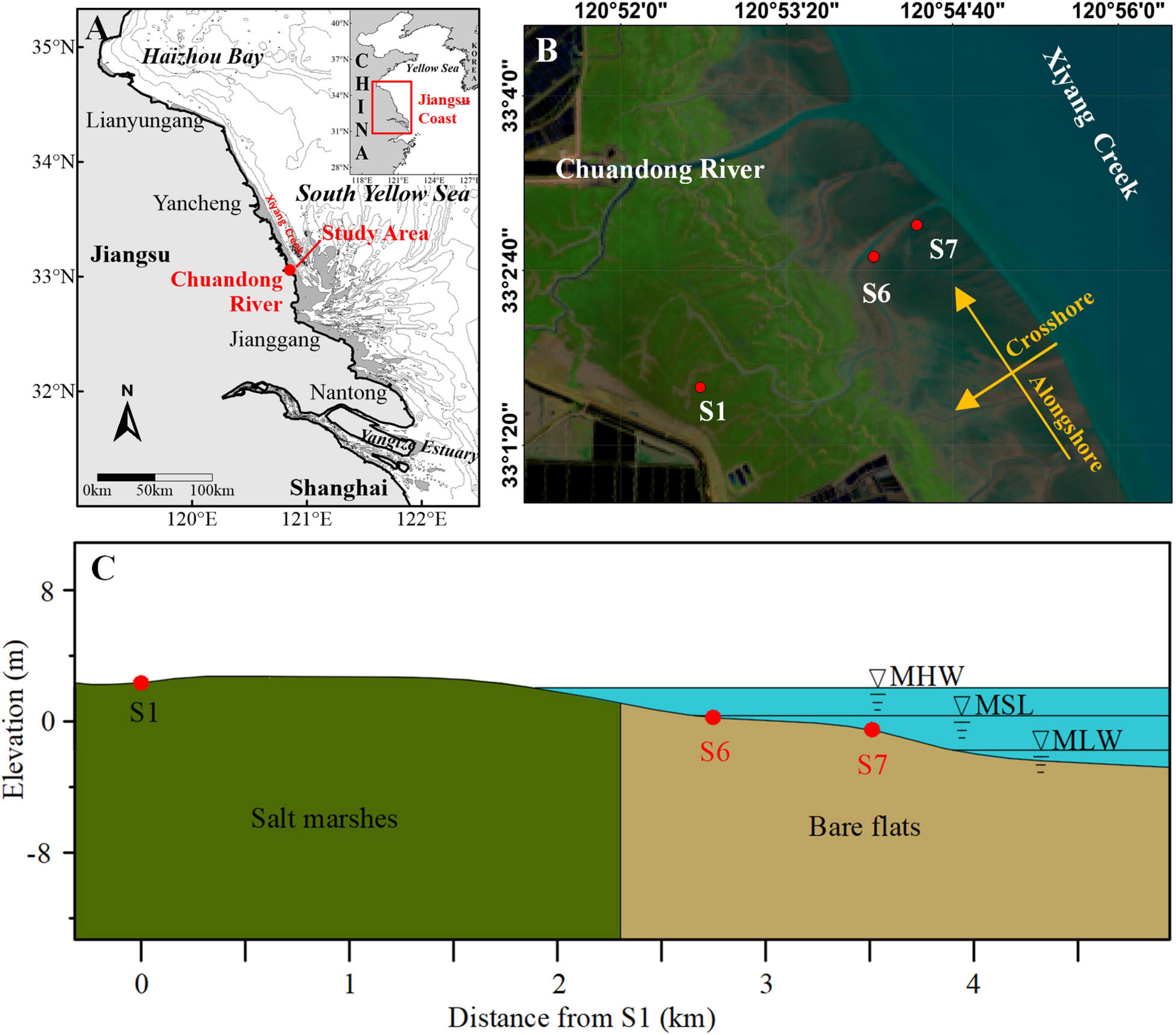
Figure 1. Location of the study area and the observation stations. (a) The study area was located at the central Jiangsu coast, China; (b) Satellite image of the study area in 2015, joint hydrodynamic and sediment measurements were collected at S6 and S7; (c) Cross section of the intertidal and supratidal mudflat profile, based on elevation data collected in December 2015.

Methods

Ethics Statement

Written informed consent was obtained from the individuals for the publication of any potentially identifiable images or data included in this article.

Field Campaigns

Our cross-shore field surveys were conducted on a tidal flat to the south of the Chuandong River from December 24 to 26, 2015 (Figure 1b). These locations were selected based on previous studies of the long-term elevation change at nine observational stations along a cross-shore profile perpendicular to the shoreline (Gong et al., 2017). Stations S6 and S7, which are among the nine stations, are located on unvegetated intertidal flats. The distance of the two stations to S1, which is located on the upper intertidal flats and is close to the sea dyke, are shown in Figure 1c. At each observation station, a custom observation system was deployed to measure synchronously water depth, and vertical profiles of three components of velocities and SSC. The system was previously used in the study area and the data quality was proven to be good (Zhang et al., 2016a).

Instruments were mounted from poles, extending 4 m (Station S6) and 5 m (Station S7) above bare flats (Figures 2a,b). The Nortek Vectrino Profiler was installed 7 and 10 cm above the initial bed at Station S6 and S7, respectively, to capture near bottom velocity profiles at 25 Hz continuously with a range of 3.5 cm and a resolution of 1 mm (35 layers in total). Since the highest velocity measurement was 4 cm below the transducer, effective velocity profiles ranged 0–3 cm above bed at Station S6 and 2.5–6 cm above bed at Station S7 at installation. The Vectrino also recorded the distance between the transducer and bed surface at a frequency of 1 Hz. Turbidity was measured at five elevations, 5, 25, 60, 120, and 200 cm above the bed, respectively, using self-contained OBSs (OBS 3A and OBS 5+). The OBS at 2 m at Station S6 failed to record data because it was never inundated. Tide and Wave Recorders (refer to Table 1 for details about the instruments) measured water depth and wave properties every 5 and 30 min, respectively. Different instruments were used at the two stations to measure the velocity profile over the entire water column. At Station S6, a 2400 kHz ADCP was deployed in a triple-hulled vessel with its transducer looking downward. The vessel was anchored on the mudflat so that it could rise and fall with the tides, remaining within a radius of 3 m. However, it was a pity that this ADCP did not work well during measurements. Thus, the data were not used in this manuscript. At Station S7, a 2 MHz Aquadopp Profiler was buried flush with the bed with the transducer looking upward. The blanking area and the resolution of the Aquadopp are 20 and 10 cm, respectively. The heights of all instruments are illustrated in Figures 2c,d.

FIGURE 2

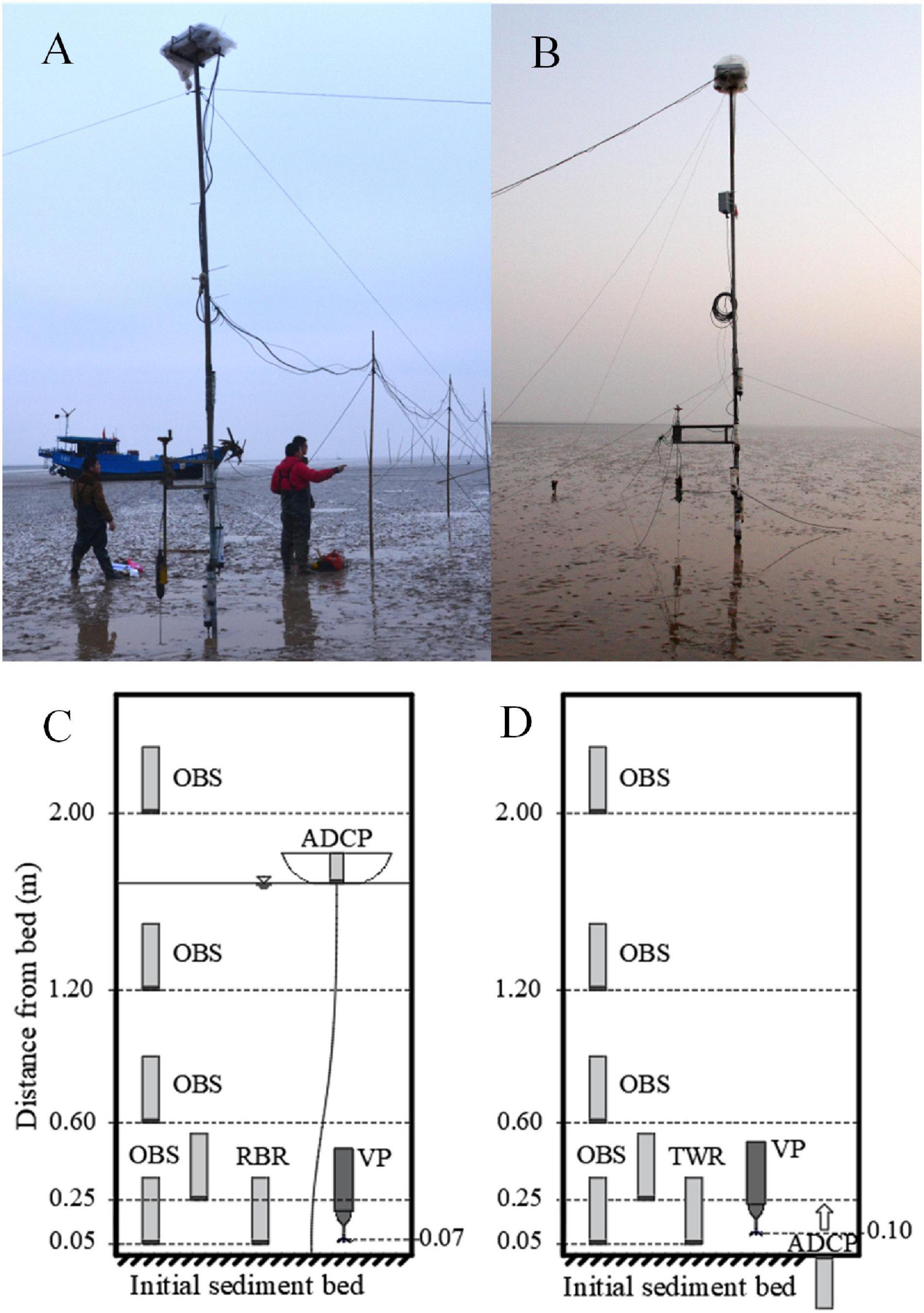
Figure 2. Measuring systems were set up at (a) Station S6 and (b) Station S7. The initial position of instruments with respect to the seabed at Station S6 and S7 are shown in panels (c,d), respectively. VP in the panels is short for Vectrino Profiler.

TABLE 1

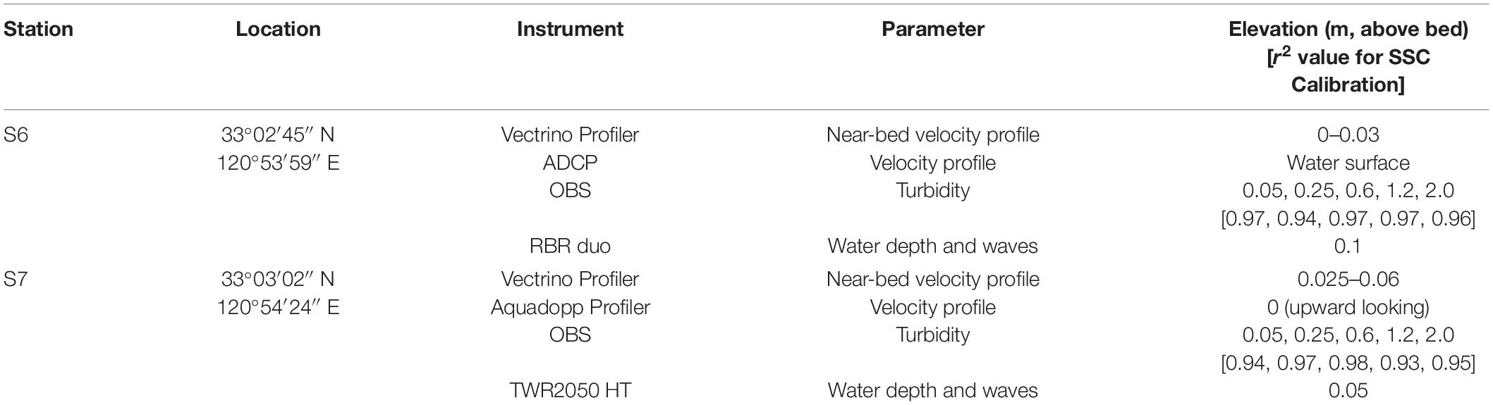
Table 1. Instruments deployed at each station and the calibration of SSC for various instruments.

Since taking water samples at the same depth as each OBS during the time-series measurements was difficult, calibration data for the OBSs were collected before installation. Water samples were collected at about 20 cm beneath the water surface while OBSs were recording turbidity at the same depth. This approach for calibration assumes that suspended sediment size varied little with time and depth, which is supported by the majority of grain size analyses of water samples taken at different depths. For the initial flood period when grain size may change because of resuspension, additional water samples were taken to check the calibration of OBSs and to document the grain size of suspended sediment. Deployment information and correlation coefficient for OBSs are listed in Table 1.

Water samples were taken for particle size distribution analysis at different elevations at five phases (the beginning of flood, peak flood, high slack, peak ebb, and the end of ebb) of each tidal cycle when instruments were collecting data. Surficial bed sediment samples were taken during each low-tide when the tidal flats were exposed.

Wave Characteristic Extraction From High-Frequency Velocity

Significant wave height (H_s), wave period (T_s), and wave direction were calculated for each 3-min segment of the high-frequency velocity data from Vectrino Profiler using spectrum method (Madsen, 1994; Wiberg and Sherwood, 2008; MacVean and Lacy, 2014):

$$T_s=\frac{\sqrt{2{\sum }_i{S}_{xx}\mathrm{\Delta }{f}_i}}{{\sum }_i{f}_i{S}_{xxi}\mathrm{\Delta }{f}_i}(1)$$

$$H_s=4{\left(\sum _i\frac{{\left(S_{xx}+S_{yy}\right)}_i\mathrm{\Delta }{f}_i}{{\left(\frac{2\mathrm{\pi }{f}_{i}cosh\left(k_{i}Z\right)}{sinh\left(k_{i}h\right)}\right)}^2}\right)}^{1/2}(2)$$

where S_xx, S_yy indicate the velocity power spectral density in x and y directions; f is the frequency of wave motion; Z is the distance above the bed at which the velocity was measured; h is water depth; and k is the wave number.

Wave-Turbulence Decomposition

Since the velocity profiles collected at station S6 were extremely adjacent to the bed, they deviated from a logarithmic distribution expected in the current boundary layer, due to the influence of the viscous sublayer and wave boundary layer. We used the TKE method to estimate bed shear stress, which requires three components of high-frequency velocity at one elevation near the bed. The velocities from the 11th layer (Brand et al., 2016) were used in TKE method for both stations.

The high-frequency velocities recorded by Vectrino Profiler are combinations of velocities from mean currents, wave motions and turbulence: $u=\overline{u}+\tilde{u}+u^{\prime }$, where u is measured velocity, $\overline{u}$ is burst mean velocity, $\tilde{u}$ is wave-induced velocity, and u′ is turbulent velocity. Determination of current-induce bed shear stress requires decomposition of these components, especially removing wave contaminant from turbulence, since waves are often more energetic than turbulent eddies in areas with large wave condition. There are several methods of decomposition (Benilov and Filyushkin, 1970; Trowbridge, 1998; Bricker and Monismith, 2007), among which the “Phase Method” raised by Bricker and Monismith (2007) is the most suitable way for this study since it requires only one point measurement of high-frequency velocity (MacVean and Lacy, 2014). This is a spectral method that assumes equilibrium turbulence and no wave–turbulence interaction, which linearly interpolates the power spectral density in log space over the designated wave frequency range. It was proved to produce better results than those produced by simple removal of the wave peak via bandpassing. Detailed steps of the method refer to Bricker and Monismith (2007). In the analysis, since the range of wave frequencies varied between bursts, we applied a fixed low-frequency cutoff and a burst-specific high-frequency cutoff, which was determined as the highest frequency of waves able to penetrate to the bottom for the burst-mean depth.

Bed Shear Stresses Induced by Currents and (or) Waves

Various methods have been developed to estimate the current-induced bed shear stress (Soulsby, 1983; Dyer, 1986; Stapleton and Huntley, 1995; Shi et al., 2012). Results using different methods may differ largely from each other, since lots of interference factors (e.g., waves, stratification) may lead to a deviation from the theoretical value (Grant and Madsen, 1986; Biron et al., 2004). Secondary momentum methods of TKE, TKEw, and RS were suggested to give more reliable estimations under the wave condition (Kim et al., 2000; Salehi and Strom, 2012; Zhang et al., 2018) and the variations of these methods were limited (Zhu, 2017). Thus, the TKE method is used to calculate the current-induced bed shear stress here.

Bottom shear stress due to currents, τ_c, can be calculated through TKE method, as follows (Soulsby, 1983):

$$Current-inducedbedshearstress:{\mathrm{\tau }}_c=\mathrm{\rho }{u}_{*}^2(3)$$

$$TKEmethod:u_{*}={\left(0.19E\right)}^{0.5}(4)$$

$$TheturbulentkineticenergyE=0.5(\overline{u^{{}^{\prime }2}}+\overline{v^{{}^{\prime }2}}+\overline{w^{{}^{\prime }2}})(5)$$

where u_* is the friction velocity, u′, v′, w′ are turbulent velocity components in three dimensions, computed as described in section “Wave Characteristic Extraction From High-Frequency Velocity.”

Wave-induced bottom shear stress, τ_w, is calculated according to Jonsson (1966) (Eqs 6, 7).

$${\mathrm{\tau }}_w=\frac{1}{2}\mathrm{\rho }{f}_w{u}_b^2(6)$$

where ρ is the density of sea water, f_w is the friction factor which indicates the impact of bottom friction on waves and links the bottom wave orbital velocity u_b with the bottom shear. For the smooth laminar flow regime (i.e., wave Reynolds number Re_w = A²ω/υ < 5×10⁵, where A = u_bT/2πandω = 2π/T, the maximum is 9.9 ×10⁴ during measurements), the friction factor is a function of the wave Reynolds number (Nielsen, 1992): $f_w=2R{e}_w^{-0.5}$ The bottom wave orbital velocity u_b was determined from wave height and period based on linear wave theory:

$$u_b=\frac{\mathrm{\pi }{H}_s}{T_{s}sinh\left(kh\right)}(7)$$

where k = 2π/L is the wave number, $L=g{T}_s^2/2\mathrm{\pi }\times tanh\left(kh\right)$ is the wave length, H_s is the significant wave height; and T_s is the significant wave period, which can be calculated from Eqs 1, 2, h is the water depth, and g is the acceleration due to gravity.

Several models have been developed to evaluate the bottom shear stress under both current and wave conditions. Equations from Soulsby (1995) are recommended to calculate the mean and maximum bottom shear stresses (Eqs 8, 9).

The Cycle-mean bed shear stress τ_m can be calculated through the following equation:

$${\mathrm{\tau }}_m={\mathrm{\tau }}_c\left[1+1.2{\left(\frac{{\mathrm{\tau }}_w}{{\mathrm{\tau }}_c+{\mathrm{\tau }}_w}\right)}^{3.2}\right](8)$$

Based on the assumption that the enhancement of the oscillatory component of stress caused by the current-induced turbulence is negligible, the maximum value of bed shear stress τ_max can be calculated by:

$${\mathrm{\tau }}_{max}={\left[{\left({\mathrm{\tau }}_m+{\mathrm{\tau }}_w\left|cos\mathrm{\varphi }\right|\right)}^2+{\left({\mathrm{\tau }}_w\left|sin\mathrm{\varphi }\right|\right)}^2\right]}^{1/2}(9)$$

where ϕ is the angle between current direction and direction of wave travel.

Since wave parameters were calculated every 3 min, wave and current stresses were calculated once every 3 min as well.

Suspended Sediment Flux and Bed Level Change

The instantaneous suspended sediment flux per unit width (SSF,kg/(m⋅s)) on tidal flats is the integral from the bed to the water surface of the product of the instantaneous velocity and instantaneous sediment concentration, both of which vary with elevation above the bed. In this study, SSC and velocity (from Aquadopp Profiler and Vectrino Profiler) data were collected at discrete elevations throughout the water column. In the 20 cm-range area above the bottom, velocity profiles were extended from the 3 cm-range using logarithmic fitting. For the upper water column, velocity was assumed to be uniform within each 10-cm layer. The SSF was estimated by summing these layer-averaged values:

$$SSF=\sum _0^n\overline{u_i}\overline{c_i}{h}_i(10)$$

where n is the number of layers used in the calculation, h_i is the thickness of layer i, $\overline{u_i}$ is the depth-averaged velocity of layer i, and $\overline{c_i}$ is the depth-averaged SSC of layer i. As illustrated by the arrows in Figure 1b, positive cross-shore flux indicates landward net transport, and positive long-shore flux indicates northwestward along-shore transport. Finally, integrating SSF for portions of the tide gave a net movement of sediment at different tidal stages.

Bed elevation change, ΔD, was calculated from the time-series distance D_t (from the transducer to the bed surface) recorded by the Vectrino Profiler:

$$\mathrm{\Delta }D=D_t-D_{t+1}(11)$$

Negative values of ΔD indicate erosion and positive values indicate deposition.

Results

Cross-Shore Variations of Waves and Currents

Three tidal cycles (numbered as 6-1, 6-2, and 6-3 for Station S6; 7-1, 7-2, and 7-3 for Station S7 hereafter) when instruments performed well and data return was high were selected for analysis in this paper. Water depth and significant wave heights are presented in Figure 3. The significant wave heights were calculated from high-frequency velocity data based on Eq. 2.

FIGURE 3

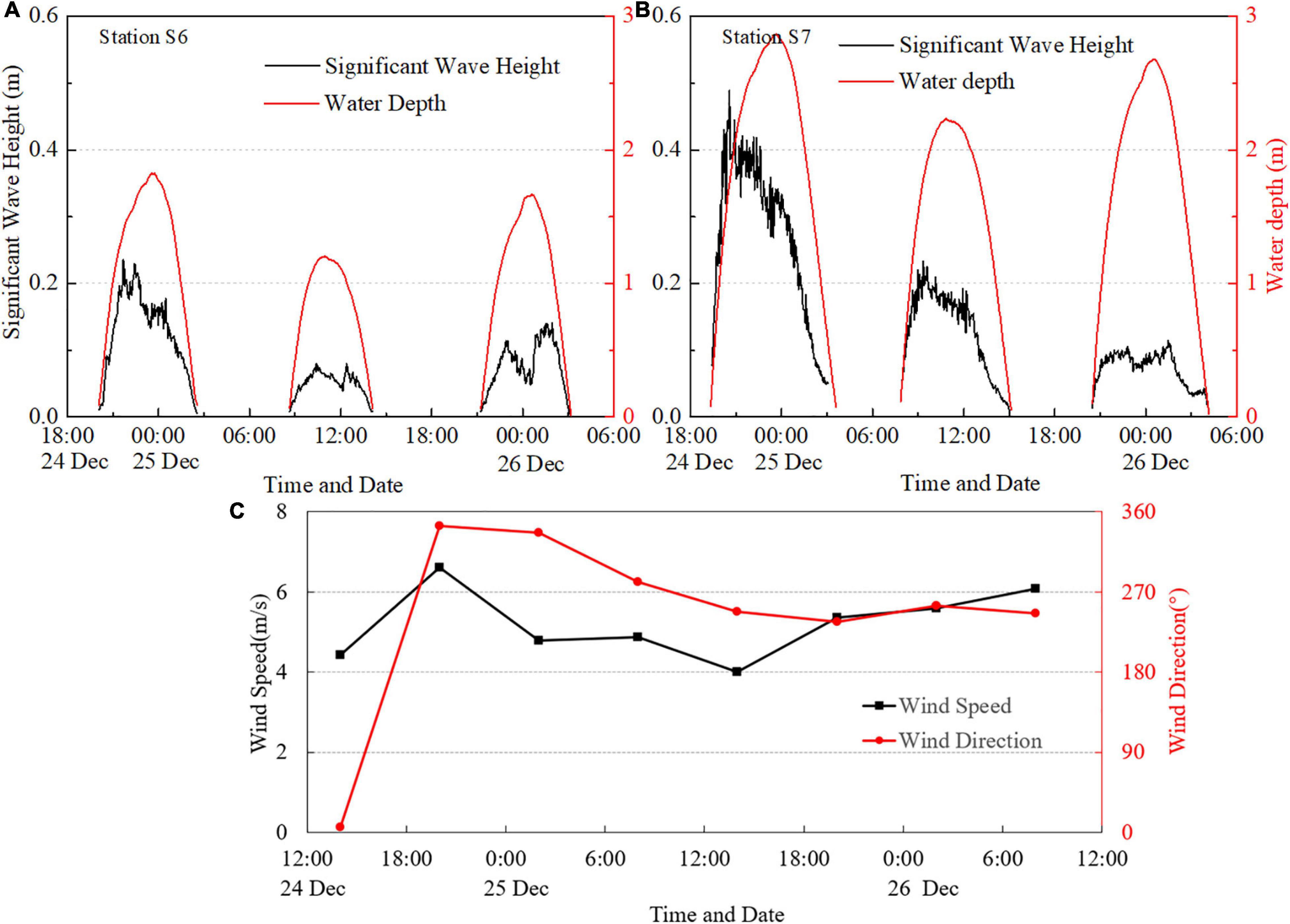
Figure 3. Measured water depth and significant wave height at (A) Station S6 and (B) Station S7, respectively. Wind speed and direction during measurements are shown in panel (C). The dataset of wind is from CCMP.

The maximum water depth was 1.82 m at Station S6 and 2.87 m at Station S7. The average inundation time at Station S7 was 7.9 h, which was 1.75 h longer than that at Station S6. Wave heights at Station S7 were generally larger than that at Station S6 due to landward wave attenuation in most cases. A cold wave event with a maximum wind speed of 6.6 m/s attacked the study area during the night of December 24 [Figure 3C, the wind data was from the Cross-Calibrated Multi-Platform (CCMP), which is provided by the NASA PO.DAAC], resulting in strong landward wind and large waves, with wave heights at Station S7 as high as 0.49 m. In the last event, wave heights at Station S6 were mostly larger than at S7 since the wind direction changed to about 270° (i.e., west, nearly offshore).

The rate of water level change (dη/dt), as well as 1-min averaged flow velocity vectors at approximately 3 cm above the bed surface at both stations, here termed near-bed, are shown in Figure 4. Since bed level changed during measurements, with a maximum variation of about 1 cm, the heights of the velocity are referenced to the original bed level at time of installation.

FIGURE 4

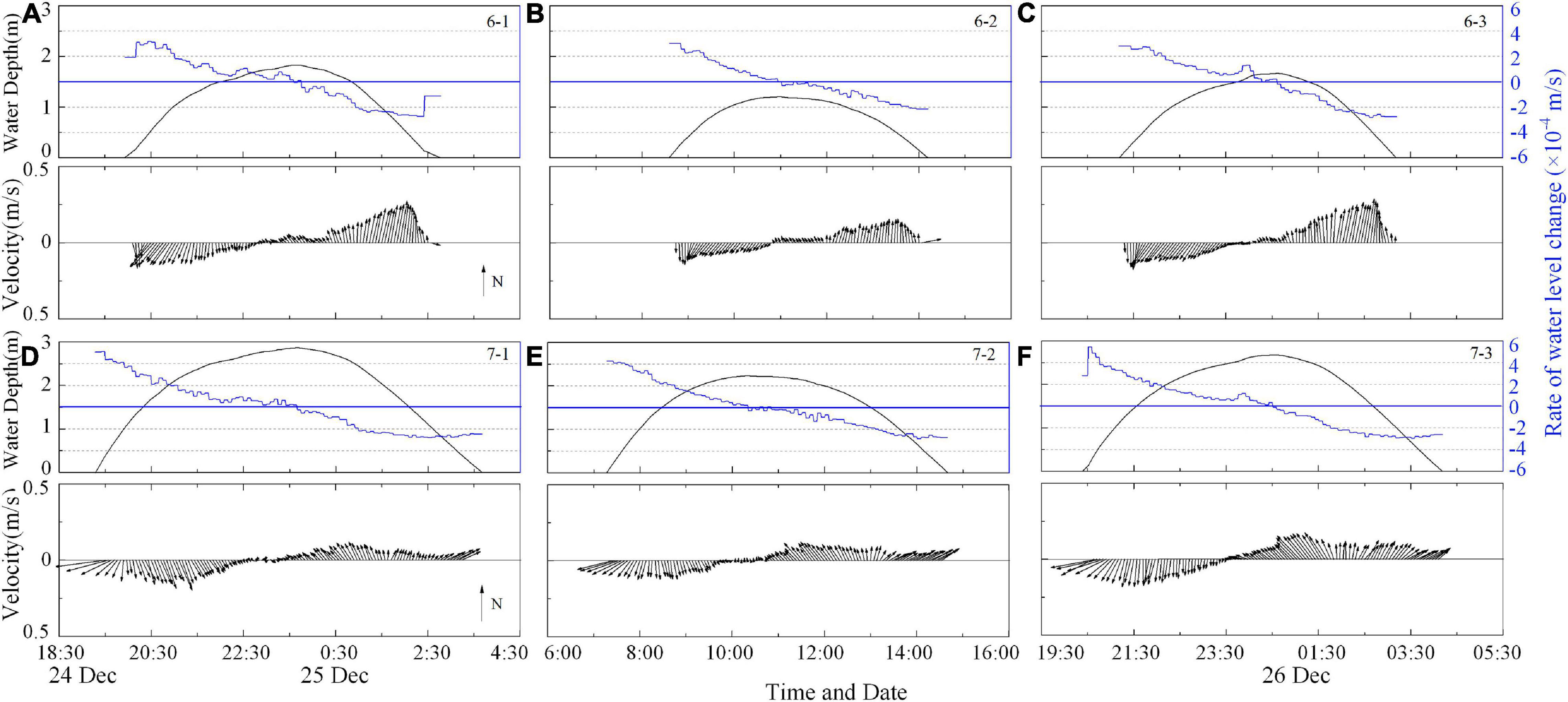
Figure 4. Water depth (black line), the rate of water level change (dη/dt, blue line) and 1-min averaged near-bed flow velocity vector at Station S6 (A–C) and Station S7 (D–F) in three tidal cycles during December 24–26, 2015.

Tidal currents at Station S6 were nearly rectilinear, and the maximum current speed at ebb was larger than at flood. At Station S7, the largest current speed was found at the beginning of each tidal cycle, which indicated that strong surges occurred during the periods of very shallow water. Flow at this station rotated anti-clockwise during flood and clockwise during ebb. Both flood and ebb tidal fronts were controlled by the bathymetry of the tidal flats, and were directed nearly perpendicular to the shoreline. During other periods rather than very shallow water, flow direction at S7 were alongshore, which was influenced by horizontal tidal circulations.

Suspended Sediment Concentration, Bed Sediment and Bed Level Changes

Suspended sediment concentration at Station S7 was much greater than at Station S6, especially near the bed (Figure 5). The average SSC at approximately 5 cm above the bed during these three tidal cycles was 0.95 g/l at Station S6, while at station S7 it was 2.26 g/l. Suspended sediment in the water column was well-mixed most of the time, especially at Station S6, except at slack water. During slack water there were strong decreases in SSC in the upper water column and increases in lower water column. At these times the decrease in vertical mixing due to weak currents leads to the development of strong vertical stratification.

FIGURE 5

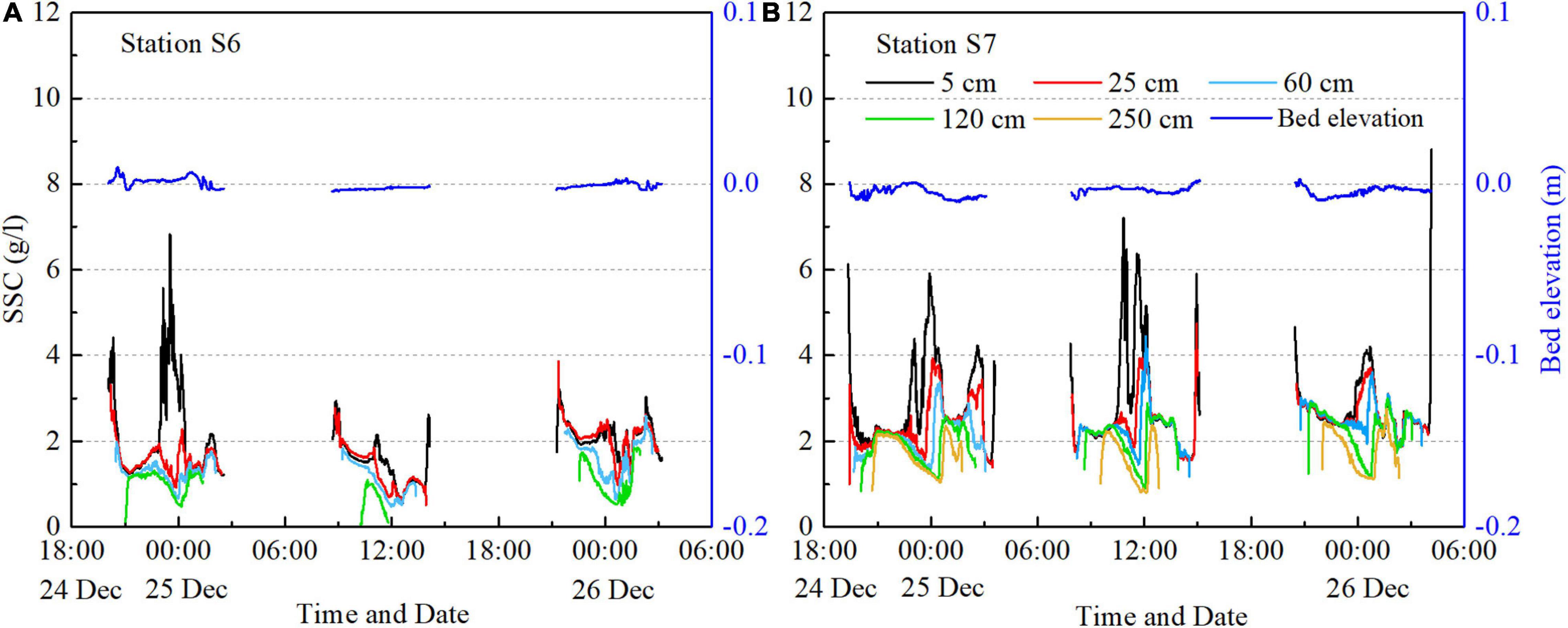
Figure 5. Stratified suspended sediment concentration and relative bed level changes at Station S6 (A) and Station S7 (B) during December 24–26, 2015.

Bed sediment at Station S6 was almost the same as S7. At middle and lower intertidal mudflats, surficial bed sediment mainly consisted of silt. The average median grain size during measurements at Station S6 and Station S7 were 23 and 27 μm, respectively. The percentages of clay (<2 μm) and silt (2–62.5 μm) at Station S6 were 7 and 86.6%, which are slightly higher than at Station S7.

The time series of distance from the transducer to bed surface was recorded by Vectrino Profilers at both stations, and the relative bed level is calculated relative to the first recorded data in the first tidal cycle (Figure 5). Previous studies showed that the fluid mud layer or the near-bottom high-concentrated sediment layer may influence the acoustic instruments to detect the real sea bed (Jaramillo et al., 2009; Sahin et al., 2012; Mehta et al., 2014). However, in our study area, the fluid mud layer is very unlikely to develop since the bed sediment was not that muddy and bed forms were extensively distributed (Winterwerp and Van Kesteren, 2004; Yao et al., 2015). In addition, the bed level data was carefully checked to exclude the influence from the near-bottom high-concentrated sediment layer. Results shown in Figure 5 indicates that the maximum bed level changes during one tidal cycle were about 1.2 cm at Station S6 and 1.3 cm at Station S7, while the net bed level changes were all less than 1 cm. It is notable that during some periods at the flood stage (e.g., around 25 December at 21:00 in Station S7), bed level dropped obviously while the SSC decreased. According to the calculated total suspended mass and suspended sediment fluxes (see Supplementary Material), which also increased significantly during this period, it is suggested that the sediment resuspended from the bed was diluted quickly throughout the water column and then brought away by the following tidal currents, since the water depth was increasing rapidly at that stage.

Bed Shear Stress Due to Current and Waves

Figure 6 shows the bed shear stress due to currents only, waves only and combined currents and waves. Currents accounted for most of the combined bed shear at Station S6. At Station S7, larger waves elevated the combined shear stress significantly, especially during the first tidal cycle, when the wave-induced bed shear stress was almost the same magnitude as the tide-induced shear stress (Figure 6B). In addition, waves played a more important role when the current was relatively weak at slack water. Therefore, sediment settling out of the upper water column due to weak currents is retarded by waves near the bed, resulting in extremely high SSCs just above the bottom (e.g., during slack period in Figure 5).

FIGURE 6

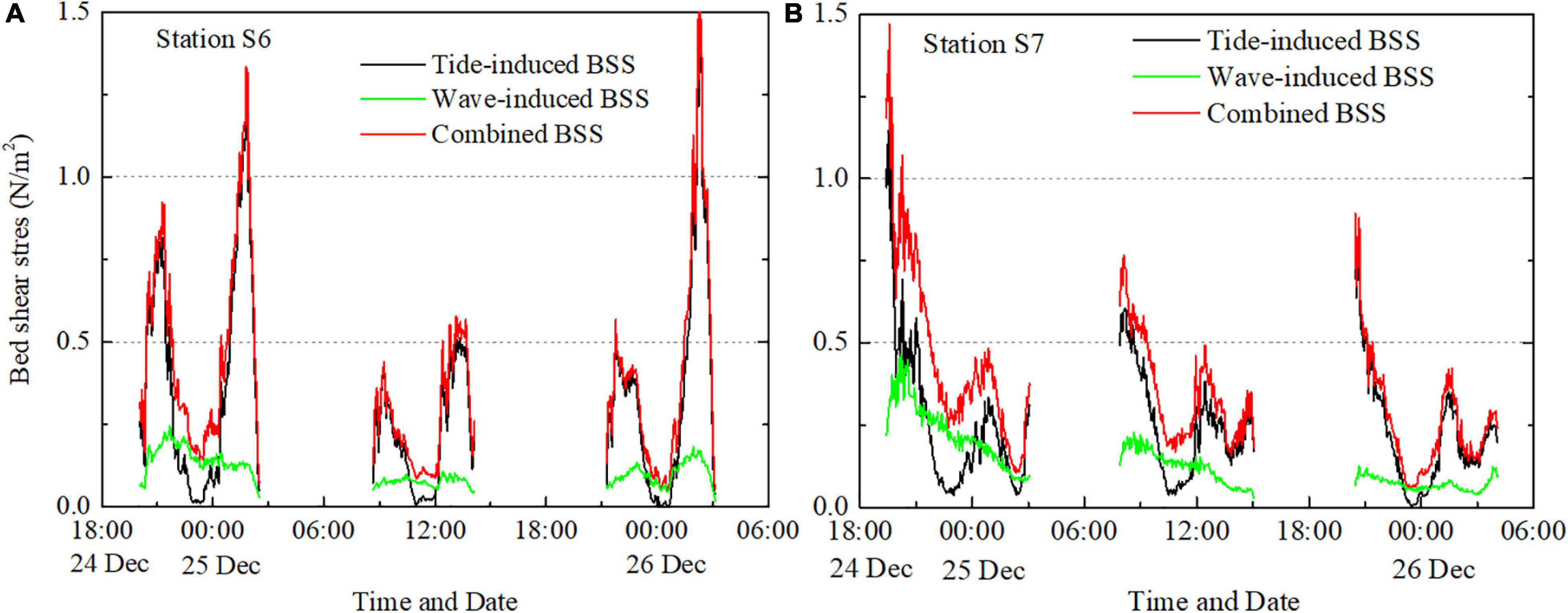
Figure 6. Tide-induced (black line), wave-induced (green line), and combined (red line) bed shear stress in Station S6 (A) and Station S7 (B).

In our study area, the critical shear stress for local sediment was measured using an in-situ annular flume (Transformed from Chen et al., 2017) and estimated to be around 0.3 N/m². The combined current and wave induced bed shear stress exceeded this value most of the time, especially at Station S7, the maximum bed shear stresses during three tidal cycles all appeared in the very shallow water stages, which were much larger than that during flood and ebb peak periods.

It is also noteworthy that when the combined bed shear stress was close to zero (e.g., at the end of each tidal cycle at Station S6), there was still sediment suspended in the water column. This is because silt-clay, which is the main component of suspended sediment in this area, settles very slowly, with settling velocities estimated at 2 mm/s (van Rijn, 2007). As a result, there was a background concentration of fine sediment advected by the tidal currents, which varies little with local hydrodynamic conditions.

Spatial Variation of Flood Surges at Middle and Lower Tidal Flats

As mentioned above, periods of very shallow water had different hydrodynamics and sediment dynamics compared to other periods. Since surges during flood period are usually more typical, only flood surges are followed with interest in this paper. To explore tidal variation in velocity and SSC, velocities and SSC are plotted as a function of water depths at Stations S6 and S7 in Figure 7. Differences can be seen between stations and among tidal cycles.

FIGURE 7

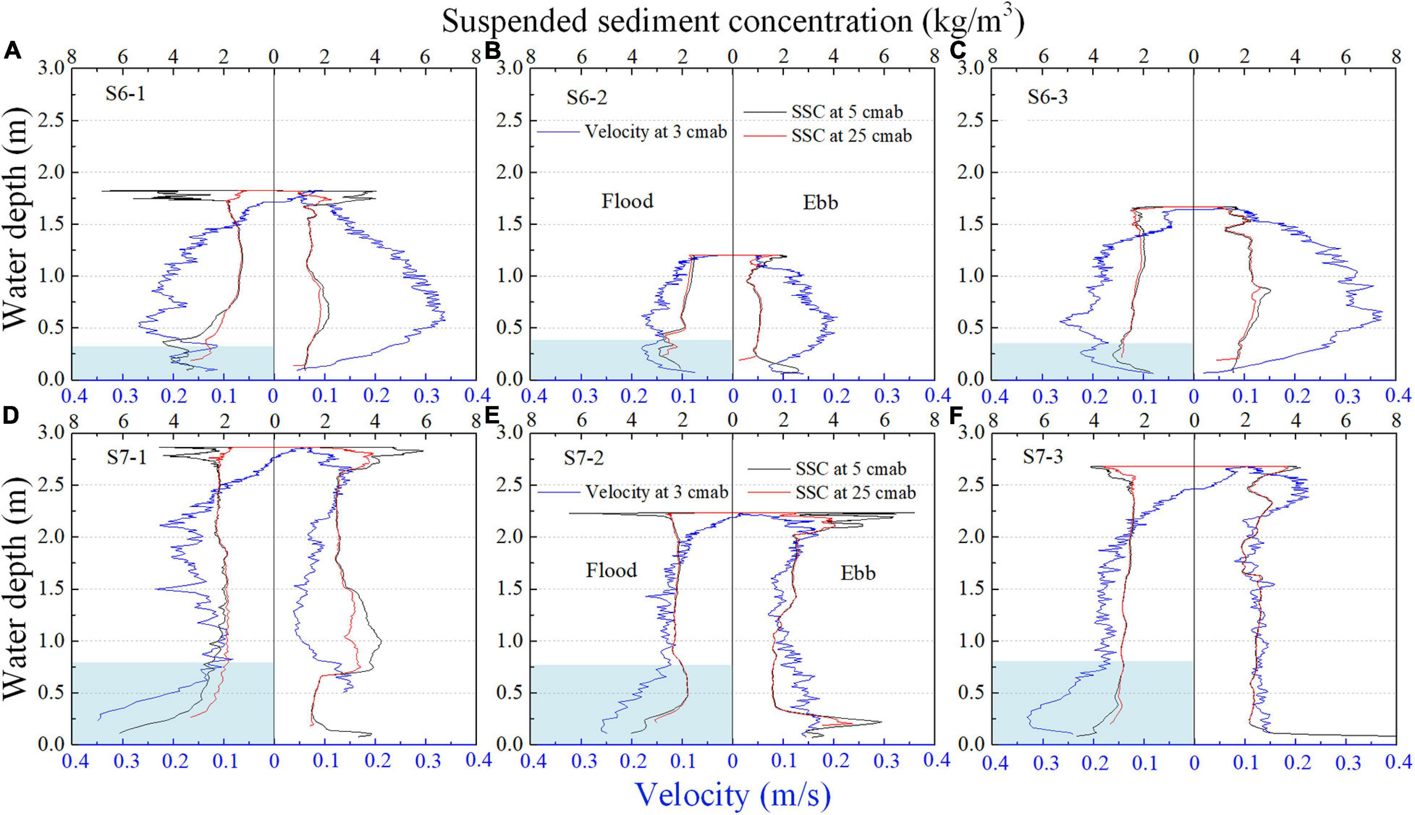
Figure 7. Relationships of near-bed velocity (blue line) and SSC (black line and red line, 5 cm above bed and 25 cm above bed, respectively) with water depth at Station S6 (A–C) and Station S7 (D–F) during three tidal cycles. The surge processes with onshore directions is highlighted with light blue shade. At Station S7 velocity and SSC surges during shallow water periods were significant, while at Station S6 velocity increases were small, accompanied by slight SSC surges.

At station S7, which is located at the lower intertidal area, velocity and SSC surges occurred during periods of very shallow water in each tidal cycle. Velocity at the beginning of each flood was the largest of the entire tidal period. Notably, velocity surges were accompanied by SSC surges. Flood-surge events in three tidal cycles are listed in Table 2. Here, the duration of flood surge is estimated from the start of flood (water level rise from zero) to the moment surge velocity decreases to low values (indicated by the light blue areas in Figure 7).

TABLE 2

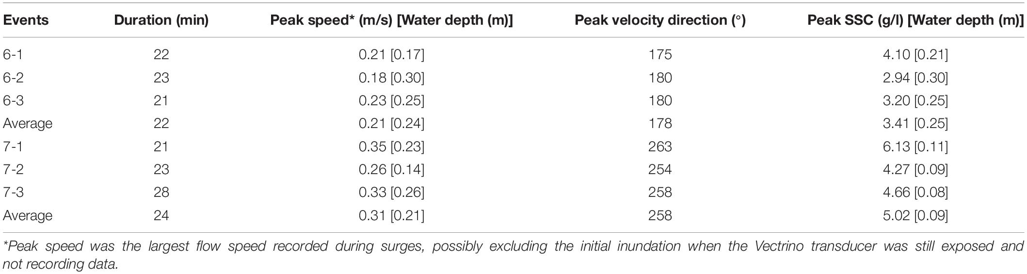
Table 2. Flood surge events at Station S6 and S7 during three tidal cycles.

Surges at Station S7 lasted more than 20 min from the initial inundation to the time velocity decreases. The peak flow of surges was directed southwestward (a general direction of 260°, which is almost perpendicular to the shoreline) at an average speed of 0.31 m/s. During surges, the peak SSC occurred prior to peak velocity (e.g., Figure 7F), which indicates that sediment suspension was intense at the tidal front current before the peak’s arrival. Therefore, during the first and second tidal cycles, the initial velocity of the tidal front might be larger than the recorded velocity peak.

Conditions at Station S6 were different from Station S7. Velocity pulses were observed during early flood, with lower magnitude at Station S6. As shown in Figures 7A–C and Table 2, the peak velocity of the surges occurred when water depth was near 20 cm, with an average value of 0.21 m/s. Since the Vectrino was installed lower at Station S6, the increasing and decreasing stages of surge velocity were fully recorded. Therefore, the peak speeds in Table 2 are considered to be the true peak velocity of surges.

Suspended Sediment Fluxes During Tidal Cycles and Flood Surges

Since the velocity data from the ADCP were not of good quality at Station S6, only SSF at Station S7 were calculated. Integrated SSF during flood surges and during both flood and ebb periods are listed in Table 3 to evaluate the contribution of surge phenomenon to suspended sediment transport at Station S7. The total SSF was in the range of 3.43–9.38 t per unit width in the cross-shore direction and 21.65–34.23 t per unit width along-shore. The along-shore suspended sediment flux was much larger than the cross-shore SSF during the whole tidal cycle, for the main direction of tidal currents was along-shore. In addition, the SSF cross-shore and along-shore varied largely among tidal cycles due to the various conditions of tides, waves and meteorology, which led to the different contribution of SSF during very shallow water stages.

TABLE 3

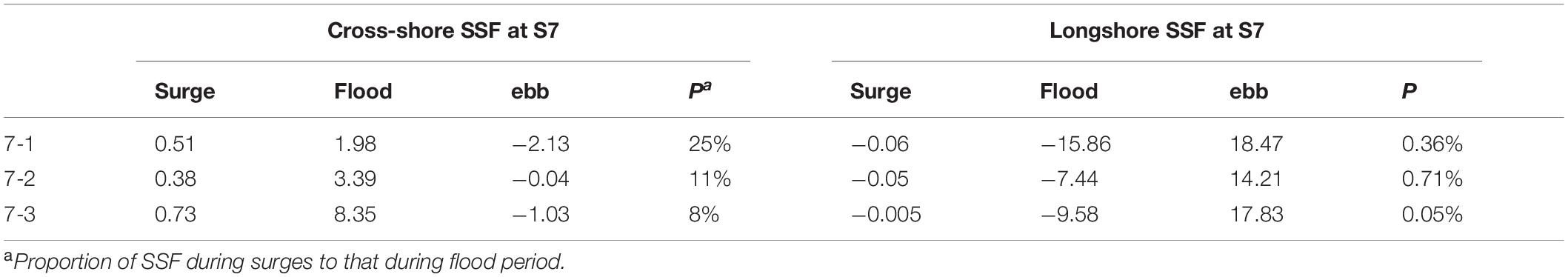
Table 3. Integrated SSF (×10³ kg/m) across and along the shoreline during different periods.

Discussion

As mentioned above, flood surges during tidal front processes on tidal flats are found worldwide (Wang et al., 1999; Gao, 2010; Friedrichs, 2011). However, questions such as which factors influence flood surges and how these surges influence sediment transport are less studied based on in-situ data. The two questions are discussed in this section, which may be helpful to understand similar phenomenon in other places.

Factors Influencing Surge Magnitude at Two Stations

According to the continuity theory, the rate of water level change and local bed slope should be responsible for the magnitude of velocity surges at tidal flats (Wang et al., 1999; Gao, 2010). At the beginning of each tidal cycle, the propagation direction of the tidal front at both stations was approximately normal to the local contour line. Therefore, the theory can be easily applied during surges, according to which the local velocity is directly proportional to the rate of water level change and inversely proportional to the local bed slope.

Figure 8 reveals the relationship between flow velocity and the ratio of water level change during flood surges. Since the 1-min data of water depth shown in the figure was linearly interpolated from the data recorded every 5 min, the rate of water level change stays the same within every 5 min, therefore resulting in a lower level of linear fitting (Figure 8). Even so, in most of the cases, higher rates of water level change contribute to larger velocities during surge stages. In addition, the linear relationship between the rate of water level change and the speed at S6 was weaker than that at S7 since the number of data used in the fitting at S6 was less.

FIGURE 8

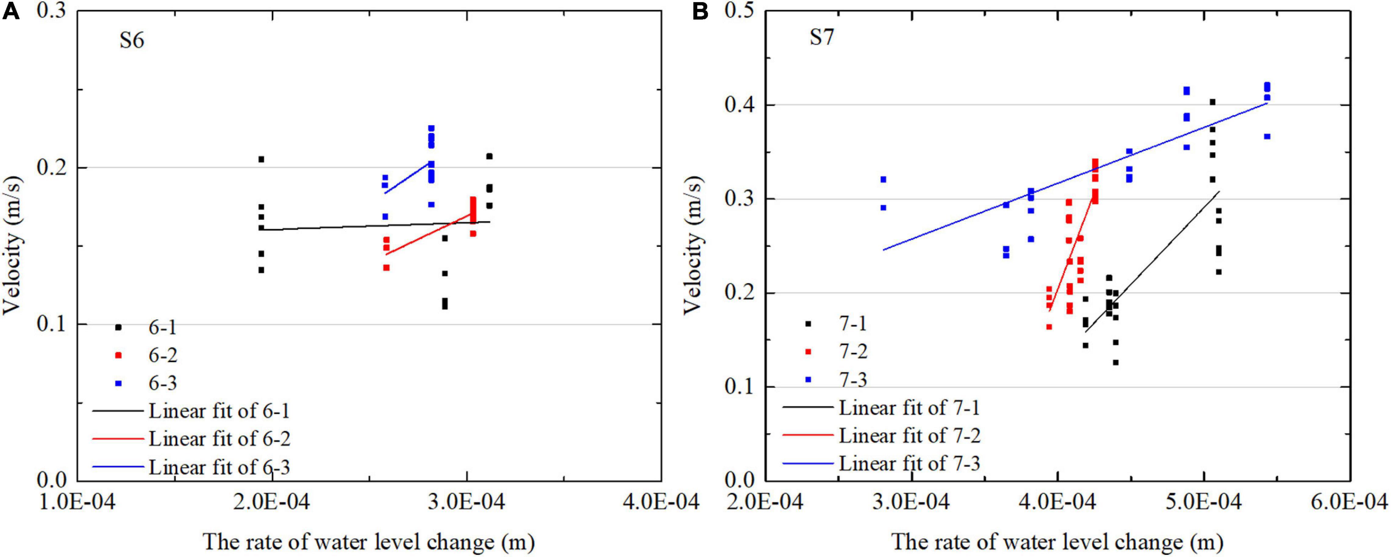
Figure 8. The relationships between the rate of water level change and the speed during surges at station S6 (A) and station S7 (B) are illustrated in dots and lines (linear fit). In most of the cases, higher rate of water level change contributes to larger velocities.

As shown in Figure 4 and Table 2, the average rate of water level changes during surges at Station S7 is 4.93 × 10^–4 m/s, which is almost 1.5 times of that at Station S6 (Table 2). According to previous study on bed elevation across this profile (Gong et al., 2017), the averaged bed slope around station S6 was approximately the same as S7 (∼0.16%). As a result of these factors, the averaged peak velocity during surges at Station S7 is higher than that at Station S6.

Compared with our earlier work using surge measurements taken in 2013 (Zhang et al., 2016a), this study documents the spatial variation of surges and the influence of surges on local sediment transport. The hydrodynamic characteristics at Station A (located between S7 and S8) in 2013 were quite different from those at Station S7 in 2015 (see Figure 6 in Zhang et al., 2016a and Figures 7A–C in this study), although the two locations were close to each other. The 2013 study took place in summer, when tidal currents were much stronger than in winter (Gong et al., 2017), which led to larger peak velocities during flood in the earlier study. However, a lower rate of water level change (only 3 × 10^–4 m/s during the surge) and larger bed slope at Station A (the slope increases toward the sea from Station S7 to Station A) led to a relatively smaller surge.

In the above discussion, the continuity theory gives a good explanation to the relative magnitude of surges occurred at different elevations. However, it’s notable that the water surface is actually not as horizontal as assumed in the continuity theory. There always exists a slope of the water surface, which is an important driver of the water level change. For a given wave height and flow speed, a larger water surface slope leads to a larger rate of water level change, resulting in a larger acceleration and surge velocity. For tidal fronts, the slope of the water surface would increase due to large bed friction where water is very shallow (Nielsen, 2018), which may also contribute to the magnitude of surges. However, related theories about deformation of tidal fronts on small-slope tidal flats are rarely found and remain to be studied.

Contribution of Flood Surges to Suspended Sediment Fluxes

Flood surges were short-duration stages and lasted for only about 24 min on average at Station S7 (Table 2), which represents about 10% of the total flood duration. However, the cross-shore suspended sediment transport during surges accounts for more than 8% of the total landward transport during flood tides, with a maximum percentage up to 25% and an average value of 15% for the three tidal cycles (Table 3). Considering the very small water depth during surges, the sediment capacity of the shallow tidal front is remarkable.

In contrast, surges contribute little to the alongshore SSF during flood tides. This is due to the change of the current direction over the tidal cycle. Currents at Station S7 were directed toward the shoreline during flood surges, and turned to long-shore direction afterward. However, resuspension and vertical mixing processes occurring during surges potentially increase the subsequent alongshore suspended sediment transport.

It is worth noting that the amount of cross-shore SSF over the entire tidal cycle varied with wave energy. Net landward suspended sediment transport was larger during the second and third tidal cycles when waves were smaller. Waves contribute to the suspension of sediment in the water and enhance the seaward transport of sediment.

It is also reasonable to speculate that the contribution of surges to total SSF at Station S6 is much smaller than at Station S7, due to the smaller velocities and SSCs during surges.

Sediment Resuspension and Morphodynamical Effects During Flood Surges

To explore the response of suspended sediment and local morphology to flow conditions, bed level changes during the whole tidal cycle and during surges were listed in Table 4. In addition, the relationship between current speed and depth-averaged SSC (Figure 9), as well as the relationship between changes in bed level and in total suspended mass per unit time (Figure 10, changes are calculated every 3 min) are also explored here.

TABLE 4

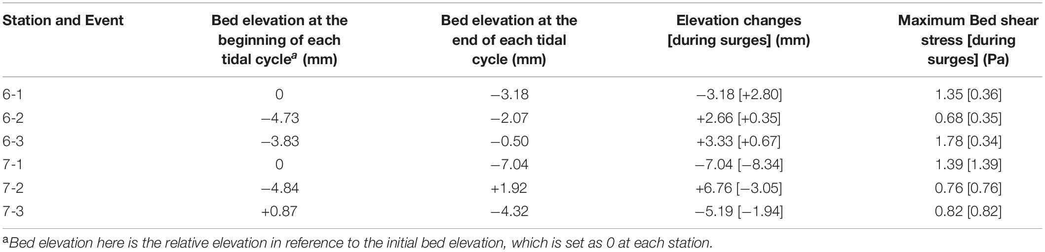
Table 4. Bed elevation changes and the maximum bed shear stress during each tidal cycle and, particularly, during flood surge evens.

FIGURE 9

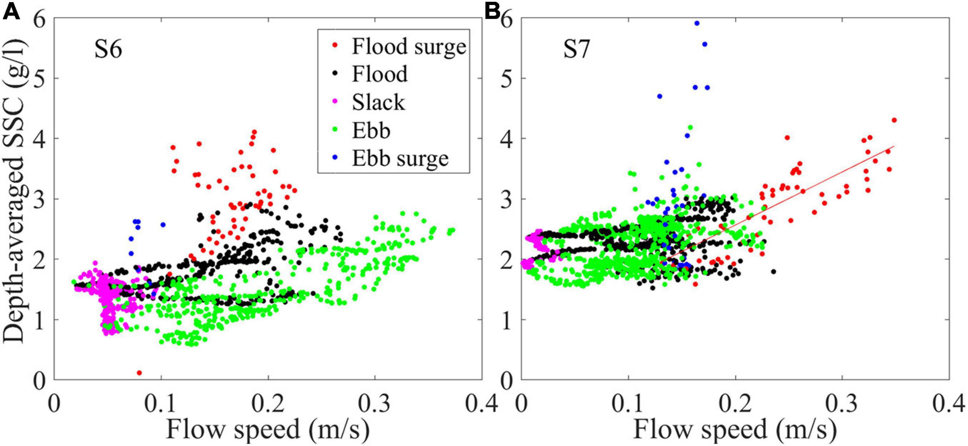
Figure 9. Relationship between near-bed flow speed and depth-averaged SSC during three tidal cycles in (A) Station S6 and (B) Station S7, in which relationship during surges is illustrated by red dots. The red line in panel (B) is a linear fitting for red dot, indicating a strong linear correlation between flow speed and SSC during surges (r = 0.8).

FIGURE 10

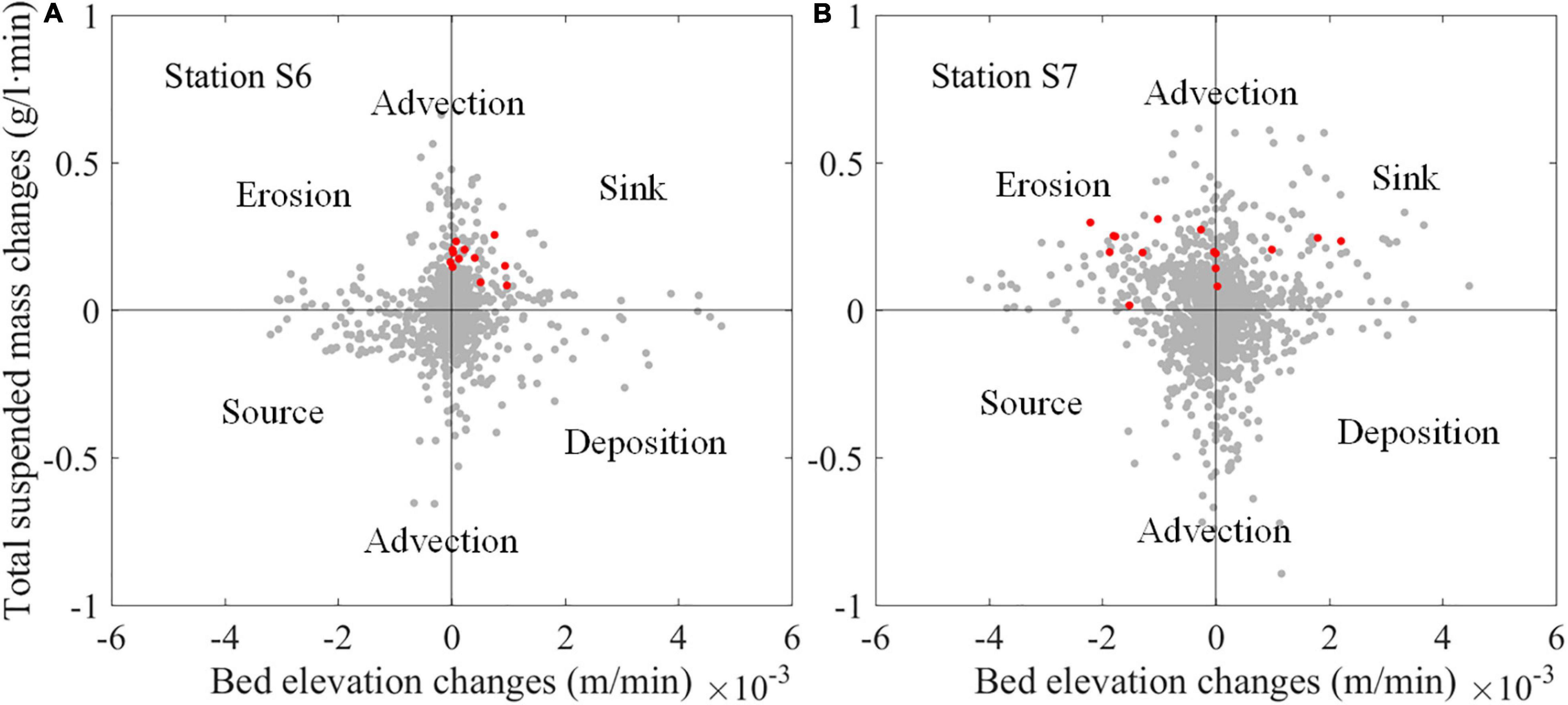
Figure 10. Relationship between the changes of bed elevation and total suspended mass in Station S6 (A) and Station S7 (B). The changes are calculated every 3 min. Red dots indicate changes during surge periods while the rest of the three tidal cycles are illustrated by gray dots.

At Station S7, the SSC responded quickly to the local hydrodynamic conditions, since a strong positive correlation between flow speed and depth-averaged SSC was exhibited (red fitting line in Figure 9B). At the same time, bed erosion occurred when the total suspended mass went up (red dots in Figure 10B, 9 out of 13 are concentrated in the fourth quadrant), and the total bed level decreased up to 8.34 mm during flood surges (Table 4), which is a direct evidence of local resuspension. Furthermore, evidence of resuspension can also be found through comparing the grain size of suspended and bed sediment (Figure 11B). The particle size distribution of suspended sediment from near the bed at initial flood was different from that at flood peak, and was more similar to that of the bed sediment.

FIGURE 11

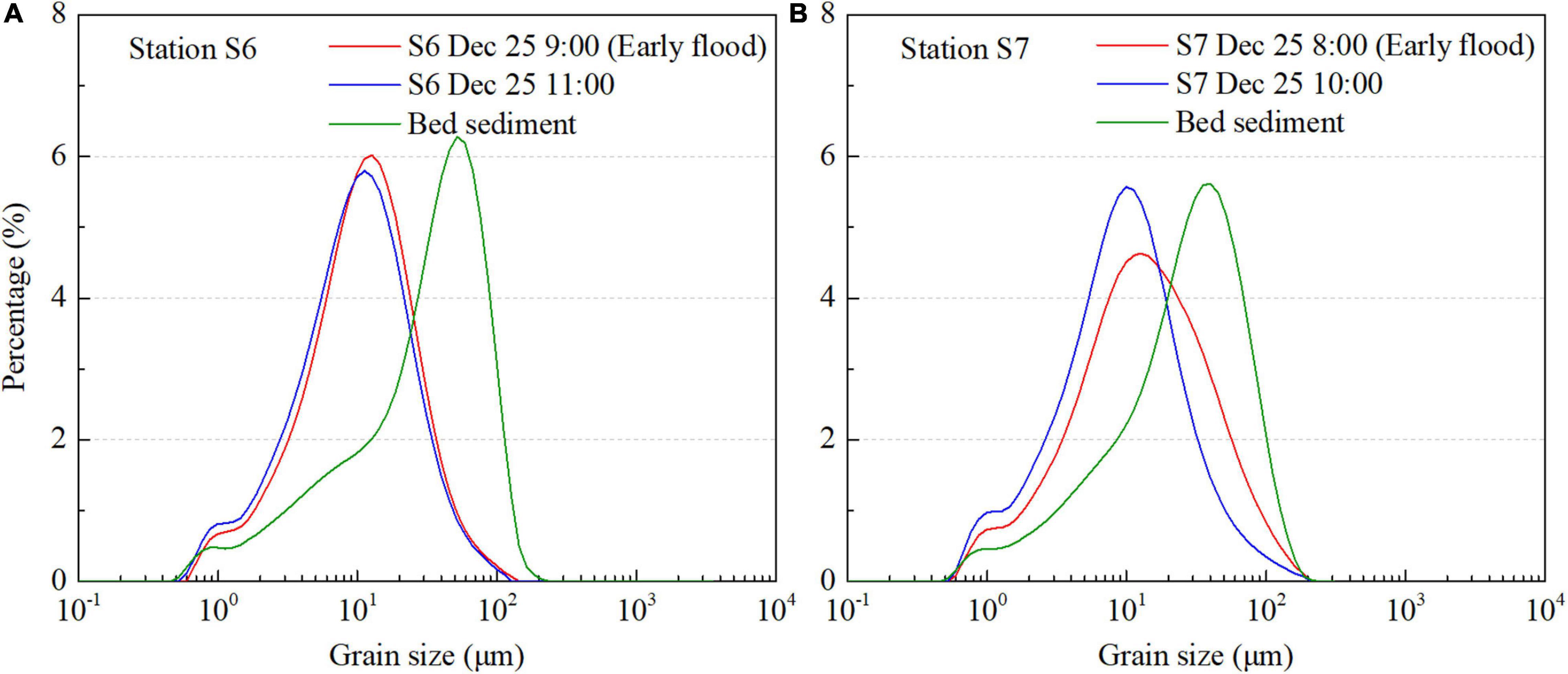
Figure 11. Grain size of bed sediment (green line), suspended sediment during early flood (red line), and flood peak (blue line) at (A) Station S6 and (B) Station S7. Water samples of suspended sediment were taken from near-bottom water column.

It is easy to understand the resuspension during flood surges at Station S7, since the bed shear stress also surged at the same time with a maximum value of 0.76–1.39 Pa in different tidal cycles (Table 4), and kept higher than 0.4 Pa during surge period, which exceeded the local critical bed shear stress (around 0.3 Pa) largely and led to strong resuspension immediately. Therefore, we suggest that resuspension occurred during flood surges at Station S7, and contributed to the increase in SSC.

There is also a relatively large SSC during tidal fronts at Station S6 (red dots in Figure 9A). However, the mechanism of the SSC surge was different from that at Station S7 since no erosion was observed during surges. In contrast, the relationship between bed level changes and total suspended mass changes (red dots in Figure 10A) indicates that tidal front water brought in large amounts of sediment, some of which was deposited at this station, with a maximum value of 2.8 mm during the surge periods (Table 4). The maximum bed shear stress during surge period was around 0.3 Pa, which was quite close to, but not larger than the critical bed shear stress. Therefore, the surge process was not strong enough for effective resuspension.

There are two possible explanations for the SSC surge during the initial flood period at Station S6. On the one hand, current direction indicates that the flood-tide surge at this station may propagate up the tidal creek, so advection from the creek may account for the high SSC during the surge. After the surge, currents were governed by the tidal front propagating across the tidal flat, which was less turbid than the tidal creek water. On the other hand, the particle size distribution of suspended sediment from near the bed at early flood was similar to flood peak but differed greatly from bed sediment at Station S6 (Figure 11A). However, we noted that after ebb tides, there was a thin layer of loose sediment covered on top of the bed at Station S6, which was not found at Station S7. It is suggested that this layer of loose sediment is suspended matters trapped from last tidal cycle and is easily suspended by the follow flood current. Therefore, the high SSC at Station S6 during the flood surge was the combined impacts from finer advected background suspended sediment and rapid resuspension of these recently deposited sediments. That is probably the reason of even a small velocity could cause high SSC.

As discussed above, flood surges are erosive on lower intertidal flats, producing local resuspension and bed level changes. Despite their short duration, flood surges are conductive to the exchange between bed sediment and suspended sediment, and lead to considerable cross-shore suspended sediment transport. It is also notable that although measurements were taken very close to the bed, there was still a vacant period just after the initial inundation and before the water depth increased to about 10 cm that no data was collected. Therefore, the real contribution of flood surges must be greater than that is discussed here.

Compared with Station S7, velocity surges are much weaker and the corresponding SSC surges are dominated by advection at the middle intertidal flats (Station S6). The lower SSC at S6 compared to S7 during peak flood suggests that sediment is deposited as the tidal front propagates up the flats. As the tidal front moves up the flats, conditions change from erosional to depositional.

Furthermore, in a longer term, erosion occurred at Station S7 while deposition occurred at S6 in winter season (Gong et al., 2017), which was consistent with that during flood surges at two stations. This maybe an indicator that the spatial variability of these surge events across the tidal flat has the potential to influence the morphology of the tidal flat. The link between the short-term surge behavior and the long-term morphological changes would be an interesting topic which requires further studies.

Conclusion

Flood surges during periods of very shallow water exist on tidal flats worldwide. This study explored the morphological effects of surge phenomenon during periods of very shallow water through near-bed measurements conducted on an intertidal mudflat. Conclusions are drawn as follows:

(1) Velocity and SSC surges are commonly occurred at both middle and lower intertidal flats during the periods of very shallow water.

(2) Flood surges on lower intertidal flats resulted in local resuspension and strong turbidity, contributing up to 25% of the onshore-suspended sediment flux during flood tides, even though they last only 10% of the flood duration.

(3) When surges travel across the flats, conditions change from erosional to depositional. On the middle intertidal flat, advection contributed more to the surges of SSC.

Data Availability Statement

The raw data supporting the conclusions of this article will be made available by the authors, without undue reservation.

Ethics Statement

Written informed consent was obtained from the individuals for the publication of any potentially identifiable images or data included in this article.

Author Contributions

QZ and ZG designed and conducted the field survey. QZ and BX performed the data analysis. QZ and XC prepared the figures and wrote the manuscript. QZ, ZG, CZ, JL, and BJ contributed to the revision of the manuscript. All authors reviewed and agreed to the final manuscript.

Funding

This work was supported by the National Natural Science Foundation of China (grant numbers: 51909073, 51879095, and 51620105005), China Post-doctoral Science Foundation (2019M661712), National Science Fund for Distinguished Young Scholars (51925905), and the Open Research Fund of State Key Laboratory of Estuarine and Coastal Research (SKLEC-KF201902).

Conflict of Interest

The authors declare that the research was conducted in the absence of any commercial or financial relationships that could be construed as a potential conflict of interest.

Acknowledgments

We would like to thank Huan Li, Hui Cai, Shanpeng Zhu, Changcai Gu, Chuang Jin, Kun Zhao, Liang Geng, Jiawei Yan, Siyu Zhu, Bingrui Liu, Yansong Zhang, and Quan Gan for their concerted efforts in technical support and fieldwork, and Yanyan Kang and Weiqi Dai for offering the satellite images. Additional thanks go to Prof. Marcel Stive, Prof. Ian Townend, and Dr. Benwei Shi for their constructive comments. Finally, the author QZ highly appreciates the funding from China Scholarship Council during her joint Ph.D. study at the USGS. Any use of trade, firm, or product names is for descriptive purposes only and does not imply endorsement by the U.S. Government.

Supplementary Material

The Supplementary Material for this article can be found online at: https://www.frontiersin.org/articles/10.3389/fmars.2021.599799/full#supplementary-material

References

Bayliss-Smith, T. P., Healey, R., Lailey, R., Spencer, T., and Stoddart, D. R. (1979). Tidal flows in salt marsh creeks. Estuar Coast. Mar. Sci. 9, 235–255. doi: 10.1016/0302-3524(79)90038-0

CrossRef Full Text | Google Scholar

Benilov, A. Y., and Filyushkin, B. N. (1970). Application of methods of linear filtration to an analysis of fluctuations in the surface layer of the sea. Atmos. Oceanic Phys. 6, 810–819.

Google Scholar

Biron, P. M., Robson, C., Lapointe, M. F., and Gaskin, S. J. (2004). Comparing different methods of bed shear stress estimates in simple and complex flow fields. Earth Surf. Process. Landform. 29, 1403–1415. doi: 10.1002/esp.1111

CrossRef Full Text | Google Scholar

Bola Os, R., Brown, J. M., and Souza, A. J. (2014). Wave–current interactions in a tide dominated estuary. Continent. Shelf Res. 87, 109–123. doi: 10.1016/j.csr.2014.05.009

CrossRef Full Text | Google Scholar

Boldt, K. V., Nittrouer, C. A., and Ogston, A. S. (2013). Seasonal transfer and net accumulation of fine sediment on a muddy tidal flat: Willapa Bay, Washington. Contin. Shelf Res. 60, S157–S172. doi: 10.5539/jgg.v10n1p109

CrossRef Full Text | Google Scholar

Boon, J. (1975). Tidal discharge asymmetry in a salt marsh drainage system. Limnol. Oceanogr. 20, 71–80. doi: 10.4319/lo.1975.20.1.0071

CrossRef Full Text | Google Scholar

Brand, A., Noss, C., Dinkel, C., and Holzner, M. (2016). High-resolution measurements of turbulent flow close to the sediment-water interface using a bistatic acoustic profiler. J. Atmosph. Oceanic Technol. 33, 769–788. doi: 10.1175/jtech-d-15-0152.1

CrossRef Full Text | Google Scholar

Bricker, J. D., and Monismith, S. G. (2007). Spectral wave–turbulence decomposition. J. Atmosph. Oceanic Technol. 24, 1479–1487. doi: 10.1175/jtech2066.1

CrossRef Full Text | Google Scholar

Carling, P. A., Williams, J. J., Croudace, I. W., and Amos, C. L. (2009). Formation of mud ridge and runnels in the intertidal zone of the Severn Estuary, UK. Contin. Shelf Res. 29, 1913–1926. doi: 10.1016/j.csr.2008.12.009

CrossRef Full Text | Google Scholar

Chen, X. D., Zhang, C. K., Paterson, D. M., Thompson, C. E. L., Townend, I. H., Gong, Z., et al. (2017). Hindered erosion: the biological mediation of noncohesive sediment behavior. Water Resour. Res. 53, 4787–4801. doi: 10.1002/2016wr020105

CrossRef Full Text | Google Scholar

Dyer, K. R. (1986). Coastal and Estuarine Sediment Dynamics. Hoboken, NJ: A Wiley-Interscience Publication.

Google Scholar

Fagherazzi, S., and Mariotti, G. (2012). Mudflat runnels: evidence and importance of very shallow flows in intertidal morphodynamics. Geophys. Res. Lett. 39, L4401–L4402.

Google Scholar

Friedrichs, C. T. (2011). “Tidal flat morphodynamics: a synthesis,” in Treatise on Estuarine and Coastal Science, eds E. Wolanski and D. McLusky (Waltham, MA: Academic Press), 137–170. doi: 10.1016/b978-0-12-374711-2.00307-7

CrossRef Full Text | Google Scholar

Gao, S. (2009). Modeling the preservation potential of tidal flat sedimentary records, Jiangsu coast, eastern China. Continent. Shelf Res. 29, 1927–1936. doi: 10.1016/j.csr.2008.12.010

CrossRef Full Text | Google Scholar

Gao, S. (2010). Extremely shallow water benthic boundary layer processes and the resultant sedimentological and morphological characteristics [in Chinese with English abstract]. Acta Sedimentol. Sin. 28, 926–932.

Google Scholar

Gong, Z., Jin, C., Zhang, C., Zhou, Z., Zhang, Q., and Li, H. (2017). Temporal and spatial morphological variations along a cross-shore intertidal profile, Jiangsu, China. Continent. Shelf Res. 144, 1–9. doi: 10.1016/j.csr.2017.06.009

CrossRef Full Text | Google Scholar

Gong, Z., Wang, Z. B., Stive, M., and Zhang, C. (2011). “Tidal flat evolution at the central Jiangsu coast, China, Asian and Pacific Coasts (APAC 2011),” in Proceedings of the Sixth International Conference on Asian and Pacific Coasts (APAC 2011) December 14–16, Hong Kong, 562–570. doi: 10.1142/9789814366489_0065

CrossRef Full Text | Google Scholar

Grant, W. D., and Madsen, O. S. (1986). The continental-shelf bottom boundary layer. Annu. Rev. Fluid Mech. 18, 265–305.

Google Scholar

Hughes, Z. J. (2012). “Tidal channels on tidal flats and marshes,” in Principles of Tidal Sedimentology, eds R. A. Dalrymple and Jr. R. W. Davis (Dordrecht: Springer Netherlands), 269–300. doi: 10.1007/978-94-007-0123-6_11

CrossRef Full Text | Google Scholar

Jaramillo, S., Sheremet, A., Allison, M. A., Reed, A. H., and Holland, K. T. (2009). Wave−mud interactions over the muddy Atchafalaya subaqueous clinoform, Louisiana, United States: wave−supported sediment transport. J. Geophys. Res. 114:C04002. doi: 10.1029/2008JC004821

CrossRef Full Text | Google Scholar

Jonsson, I. G. (1966). “Wave boundary layers and friction factors,” in Proceedings of the 10th International Conference on Coastal Engineering. Tokyo: American Society of Civil Engineers, 127–148.

Google Scholar

Kim, S., Friedrichs, C., Maa, J., and Wright, L. (2000). Estimating bottom stress in tidal boundary layer from acoustic doppler velocimeter data. J Hydraul. Eng. Asce. 126, 399–406.

Google Scholar

Lacy, J. R., and MacVean, L. J. (2016). Wave attenuation in the shallows of San Francisco Bay. Coast. Eng. 114, 159–168. doi: 10.1016/j.coastaleng.2016.03.008

CrossRef Full Text | Google Scholar

Leonardi, N., and Fagherazzi, S. (2014). How waves shape salt marshes. Geology 42, 887–890. doi: 10.1130/g35751.1

CrossRef Full Text | Google Scholar

MacVean, L. J., and Lacy, J. R. (2014). Interactions between waves, sediment, and turbulence on a shallow estuarine mudflat. J. Geophys. Res. 119, 1534–1553. doi: 10.1002/2013jc009477

CrossRef Full Text | Google Scholar

Madsen, O. S. (1994). “Spectral wave-current bottom boundary layer flows,” in Proceedings of the 24th International Conference on Coastal Engineering, Kobe, 384–398.

Google Scholar

Mariotti, G., and Fagherazzi, S. (2013). Wind waves on a mudflat: the influence of fetch and depth on bed shear stresses. Continent. Shelf Res. 60, S99–S110.

Google Scholar

Mehta, A. J., Samsami, F., Khare, Y. P., and Sahin, C. (2014). Fluid mud properties in nautical depth estimation. J. Waterw. Port Coastal Ocean Eng. 140, 210–222. doi: 10.1061/(asce)ww.1943-5460.0000228

PubMed Abstract | CrossRef Full Text | Google Scholar

Nielsen, P. (1992). Coastal Bottom Boundary Layers and Sediment Transport. Singapore: World Scientific.

Google Scholar

Nielsen, P. (2018). Bed shear stress, surface shape and velocity field near the tips of dam-breaks, tsunami and wave runup. Coastal Eng. 138, 126–131. doi: 10.1016/j.coastaleng.2018.04.020

CrossRef Full Text | Google Scholar

Nowacki, D. J., and Ogston, A. S. (2013). Water and sediment transport of channel-flat systems in a mesotidal mudflat: Willapa Bay, Washington. Continent. Shelf Res. 60, S111–S124.

Google Scholar

Pethick, J. S. (1980). Velocity surges and asymmetry in tidal channels. Estuar. Coast. Mar. Sci. 11, 331–345. doi: 10.1016/s0302-3524(80)80087-9

CrossRef Full Text | Google Scholar

Quaresma, V. D. S., Bastos, A. C., and Amos, C. L. (2007). Sedimentary processes over an intertidal flat: a field investigation at Hythe flats, Southampton Water (UK). Mar. Geol. 241, 117–136. doi: 10.1016/j.margeo.2007.03.009

CrossRef Full Text | Google Scholar

Sahin, C., Safak, I., Sheremet, A., and Mehta, A. J. (2012). Observations on cohesive bed reworking by waves: Atchafalaya Shelf, Louisiana. J. Geophys. Res. 117, 1–14.

Google Scholar

Salehi, M., and Strom, K. (2012). Measurement of critical shear stress for mud mixtures in the San Jacinto estuary under different wave and current combinations. Continent. Shelf Res. 47, 78–92. doi: 10.1016/j.csr.2012.07.004

CrossRef Full Text | Google Scholar

Schettini, C. A. F. (2002). Near bed sediment transport in the Itajaí-açu River estuary, southern Brazil. Proc. Mar. Sci. 5, 499–512. doi: 10.1016/s1568-2692(02)80036-5

CrossRef Full Text | Google Scholar

Shi, B., Cooper, J. R., Li, J., Yang, Y., Yang, S. L., Luo, F., et al. (2019). Hydrodynamics, erosion and accretion of intertidal mudflats in extremely shallow waters. J. Hydrol. 573, 31–39. doi: 10.1016/j.jhydrol.2019.03.065

CrossRef Full Text | Google Scholar

Shi, B., Cooper, J. R., Pratolongo, P. D., Gao, S., Bouma, T. J., Li, G., et al. (2017a). Erosion and accretion on a mudflat: the importance of very shallow-water effects. J. Geophys. Res. Oceans 122, 9476–9499. doi: 10.1002/2016jc012316

CrossRef Full Text | Google Scholar

Shi, B., Wang, Y. P., Yang, Y., Li, M., Li, P., Ni, W., et al. (2015). Determination of critical shear stresses for erosion and deposition based on in situ measurements of currents and waves over an intertidal mudflat. J. Coast. Res. 31, 1344–1356. doi: 10.2112/jcoastres-d-14-00239.1

CrossRef Full Text | Google Scholar

Shi, B., Yang, S. L., Wang, Y. P., Li, G. C., Li, M. L., Li, P., et al. (2017b). Role of wind in erosion-accretion cycles on an estuarine mudflat. J. Geophys. Res. 122, 193–206. doi: 10.1002/2016jc011902

CrossRef Full Text | Google Scholar

Shi, B. W., Yang, S. L., Wang, Y. P., Bouma, T. J., and Zhu, Q. (2012). Relating accretion and erosion at an exposed tidal wetland to the bottom shear stress of combined current–wave action. Geomorphology 138, 380–389. doi: 10.1016/j.geomorph.2011.10.004

CrossRef Full Text | Google Scholar

Shi, B. W., Yang, S. L., Wang, Y. P., Yu, Q., and Li, M. L. (2014). Intratidal erosion and deposition rates inferred from field observations of hydrodynamic and sedimentary processes: a case study of a mudflat-saltmarsh transition at the Yangtze delta front. Continent. Shelf Res. 90, 109–116. doi: 10.1016/j.csr.2014.01.019

CrossRef Full Text | Google Scholar

Soulsby, R. L. (1983). “Chapter 5 The bottom boundary layer of shelf seas,” in Physical Oceanography of Coastal and Shelf Seas, ed. B. Johns (Amsterdam: Elsevier Science Publishers), 189–266. doi: 10.1016/s0422-9894(08)70503-8

CrossRef Full Text | Google Scholar

Soulsby, R. L. (1995). “Bed shear-stresses due to combined waves and currents,” in Advances in Coastal Morphodynamics, eds M. J. F. Stive, H. J. De Vriend, J. Fredsœ, L. Hamm, R. L. Soulsby, C. Teisson, and J. C. Winterwerp (Delft, NL: Delft Hydraulics), 4–23.

Google Scholar

Stapleton, K. R., and Huntley, D. A. (1995). Seabed stress determinations using the inertial dissipation method and the turbulent kinetic energy method. Earth Surface Process. Landforms 20, 807–815. doi: 10.1002/esp.3290200906

CrossRef Full Text | Google Scholar

Trowbridge, J. H. (1998). Notes and correspondence on a technique for measurement of Turbulent Shear Stress in the Presence of Surface Waves. J. Atmosph. Oceanic Technol. 15, 290–298.

Google Scholar

van Rijn, L. C. (2007). Unified view of sediment transport by currents and waves. II: suspended transport. J. Hydraul. Eng. 133, 668–689. doi: 10.1061/(asce)0733-9429(2007)133:6(668)

CrossRef Full Text | Google Scholar

Wang, A., Ye, X., Du, X., and Zheng, B. (2014). Observations of cohesive sediment behaviors in the muddy area of the northern Taiwan Strait, China. Continent. Shelf Res. 90, 60–69. doi: 10.1016/j.csr.2014.04.002

CrossRef Full Text | Google Scholar

Wang, Y., Liu, Y., Jin, S., Sun, C., and Wei, X. (2019). Evolution of the topography of tidal flats and sandbanks along the Jiangsu coast from 1973 to 2016 observed from satellites. Isp. J. Photogram. Remote Sens. 150, 27–43. doi: 10.1016/j.isprsjprs.2019.02.001

CrossRef Full Text | Google Scholar

Wang, Y. P., Gao, S., Jia, J. J., Thompson, C., Gao, J. H., and Yang, Y. (2012). Sediment transport over an accretional intertidal flat with influences of reclamation, Jiangsu coast, China. Mar. Geol. 291-294, 147–161. doi: 10.1016/j.margeo.2011.01.004

CrossRef Full Text | Google Scholar

Wang, Y. P., Zhang, R. S., and Gao, S. (1999). Velocity variations in salt marsh creeks, Jiangsu, China. J. Coast. Res. 15, 471–477.

Google Scholar

Whitehouse, R. J. S., Bassoullet, P., Dyer, K. R., Mitchener, H. J., and Roberts, W. (2000). The influence of bedforms on flow and sediment transport over intertidal mudflats. Continent. Shelf Res. 20, 1099–1124. doi: 10.1016/s0278-4343(00)00014-5

CrossRef Full Text | Google Scholar

Wiberg, P. L., and Sherwood, C. R. (2008). Calculating wave-generated bottom orbital velocities from surface-wave parameters. Comput. Geosci. 34, 1243–1262. doi: 10.1016/j.cageo.2008.02.010

CrossRef Full Text | Google Scholar

Winterwerp, J. C., and Van Kesteren, W. G. (2004). Introduction to the Physics of Cohesive Sediment in the Marine Environment. Amsterdam: Elsevier.

Google Scholar

Xu, Y., and Wang, B. (1998). The mechanism and significance of flood surge along muddy tidal flat [in Chinese with English abstract]. Oceanol. Limnol. Sin. 8, 148–155.

Google Scholar

Yao, P., Su, M., Wang, Z., van Rijn, L. C., Zhang, C., Chen, Y., et al. (2015). Experiment inspired numerical modeling of sediment concentration over sand–silt mixtures. Coastal Eng. 105, 75–89. doi: 10.1016/j.coastaleng.2015.07.008

CrossRef Full Text | Google Scholar

You, Z. (2005). Estimation of bed roughness from mean velocities measured at two levels near the seabed. Continent. Shelf Res. 25, 1043–1051. doi: 10.1016/j.csr.2005.01.001

CrossRef Full Text | Google Scholar

Zhang, C., Zhang, D., Zhang, J., and Wang, Z. (1999). Tidal current-induced formation-storm-induced change-tidal current-induced recovery-Interpretation of depositional dynamics of formation and evolution of radial sand ridges on the Yellow Sea seafloor. Sci. China(Series D Earth Sci.) 9, 1–12. doi: 10.1007/bf02878492

CrossRef Full Text | Google Scholar

Zhang, Q., Gong, Z., Zhang, C., Lacy, J. R., Jaffe, B. E., and Xu, B. (2018). Bed shear stress estimation under wave conditions using near-bottom measurements: comparison of methods. J. Coast. Res. 85, 241–245. doi: 10.2112/si85-049.1

CrossRef Full Text | Google Scholar

Zhang, Q., Gong, Z., Zhang, C., Townend, I., Jin, C., and Li, H. (2016a). Velocity and sediment surge: what do we see at times of very shallow water on intertidal mudflats? Continen. Shelf Res. 113, 10–20. doi: 10.1016/j.csr.2015.12.003

CrossRef Full Text | Google Scholar

Zhang, Q., Gong, Z., Zhang, C., Zhou, Z., and Townend, I. (2016b). Hydraulic and sediment dynamics at times of very shallow water on intertidal mudflats: the contribution of waves. J. Coast. Res. 75, 507–511. doi: 10.2112/si75-102.1

CrossRef Full Text | Google Scholar

Zhang, R. S. (1992). Suspended sediment transport processes on tidal mud flat in Jiangsu Province, China. Estuar. Coast. Shelf Sci. 35, 225–233. doi: 10.1016/s0272-7714(05)80045-9

CrossRef Full Text | Google Scholar

Zhang, R. S., Shen, Y. M., Lu, L. Y., Yan, S. G., Wang, Y. H., Li, J. L., et al. (2004). Formation of Spartina alterniflora salt marshes on the coast of Jiangsu Province, China. Ecol. Eng. 23, 95–105. doi: 10.1016/j.ecoleng.2004.07.007

CrossRef Full Text | Google Scholar

Zhu, D. K., Ke, X. K., and Gao, S. (1986). Tidal flat sedimentation of Jiangsu coast [in Chinese with English abstract]. J. Oceanogr. Huang. Bohai Seas 4, 19–27.

Google Scholar

Zhu, Q. (2017). Sediment Dynamics on Intertidal Mudflats: A Study Based on in Situ Measurements and Numerical Modelling. Delft: Technische Universiteit Delft.

Google Scholar

Zhu, Q., van Prooijen, B. C., Wang, Z. B., Ma, Y. X., and Yang, S. L. (2016). Bed shear stress estimation on an open intertidal flat using in situ measurements. Estuar. Coast. Shelf Sci. 182, 190–201. doi: 10.1016/j.ecss.2016.08.028

CrossRef Full Text | Google Scholar

Zhu, Q., van Prooijen, B. C., Wang, Z. B., and Yang, S. L. (2017). Bed-level changes on intertidal wetland in response to waves and tides: a case study from the Yangtze River Delta. Mar. Geol. 385, 160–172. doi: 10.1016/j.margeo.2017.01.003

CrossRef Full Text | Google Scholar

Zhu, Q., Yang, S., and Ma, Y. (2014). Intra-tidal sedimentary processes associated with combined wave–current action on an exposed, erosional mudflat, southeastern Yangtze River Delta, China. Mar. Geol. 347, 95–106. doi: 10.1016/j.margeo.2013.11.005

CrossRef Full Text | Google Scholar