 Travis C. Tai
 U. Rashid Sumaila
 William W. L. Cheung
- 1Institute for the Oceans and Fisheries, University of British Columbia, Vancouver, BC, Canada
- 2School of Public Policy and Global Affairs, University of British Columbia, Vancouver, BC, Canada
Elevated atmospheric carbon dioxide (CO2) is causing global ocean changes and drives changes in organism physiology, life-history traits, and population dynamics of natural marine resources. However, our knowledge of the mechanisms and consequences of ocean acidification (OA) – in combination with other climatic drivers (i.e., warming, deoxygenation) – on organisms and downstream effects on marine fisheries is limited. Here, we explored how the direct effects of multiple changes in ocean conditions on organism aerobic performance scales up to spatial impacts on fisheries catch of 210 commercially exploited marine invertebrates, known to be susceptible to OA. Under the highest CO2 trajectory, we show that global fisheries catch potential declines by as much as 12% by the year 2100 relative to present, of which 3.4% was attributed to OA. Moreover, OA effects are exacerbated in regions with greater changes in pH (e.g., West Arctic basin), but are reduced in tropical areas where the effects of ocean warming and deoxygenation are more pronounced (e.g., Indo-Pacific). Our results enhance our knowledge on multi-stressor effects on marine resources and how they can be scaled from physiology to population dynamics. Furthermore, it underscores variability of responses to OA and identifies vulnerable regions and species.
Introduction
A direct consequence of elevated atmospheric CO2 concentrations is the rapid rate of ocean acidification (OA) (IPCC, 2013), causing changes to the biogeochemical composition of our world’s oceans and affecting marine ecosystem goods and services. Global sea surface pH has already decreased by 0.1 U since the Industrial R evolution, and is projected to decrease by up to 0.3 U by the year 2100 (Bindoff et al., 2019), a 10.0% increase in acidity (hydrogen concentration). Organism responses will vary across populations, taxonomic groups, and ecosystem types (Kroeker et al., 2013; Nagelkerken and Connell, 2015). Particularly, calcareous species (e.g., mussels, oysters, coccolithophore plankton, corals) are particularly vulnerable to OA as CO2 interferes with ocean pH and the saturation state of aragonite, affecting the formation of calcium carbonate (CaCO3) structures (Fabry et al., 2008; Ries et al., 2009). While less understood, OA also affects various physiological processes such as acid-base regulation, metabolism, and aerobic scope, as well as sensory abilities, reproduction, and development (Le Quesne and Pinnegar, 2012). These effects can lead to changes in population dynamics such as growth, survival, and fecundity, and ultimately affect marine ecosystem resources (Kroeker et al., 2013).
Interactions between OA and other concurrent climate change drivers (e.g., ocean warming, ocean deoxygenation) could exacerbate their impacts on marine species and ecosystems. In ectotherms, oxygen demand increases with temperature to maintain basal metabolic rates (Pörtner and Lannig, 2009). This reduces the aerobic scope (the capacity to increase aerobic metabolic rate above maintenance levels) and the relative supply of oxygen put toward other aerobic processes such as growth (Figure 1A). We see similar effects on aerobic scope with a reduction in dissolved oxygen concentration (Pörtner and Lannig, 2009). OA is proposed to operate in a similar manner, reducing the overall aerobic scope profile (Pörtner and Farrell, 2008; Figure 1A). Reducing aerobic scope can then have effects on life-history traits (Pauly and Cheung, 2017) (e.g., growth rate, maximum body size) and affect large-scale population dynamics (Cheung et al., 2011; Figure 1). However, this process is not ubiquitous and is not true for all organisms (e.g., Clark and Sandblom, 2013; Lefevre et al., 2017; Jutfelt et al., 2018); simpler alternative mechanisms for scaling physiological effects to life-history traits have yet to be proposed or identified. Studies that examined the effects of changes in multiple environmental variables on marine organisms are mostly limited to laboratory or small-scale field-based mesocosm experiments and are limited to a small number of species and ecosystems (Fabry et al., 2008; Ries et al., 2009; Alguero-Muniz et al., 2017; Doney et al., 2020), the number of environmental variables that could be controlled for as well as the limited representation of the full scope of environmental variabilities (Wahl et al., 2016). There is a call for the need to upscale the available experimental findings from OA-related experiments in terms of the number of environmental variables, species, and ecosystems (Wahl et al., 2016). Thus, it is extremely useful to use available experimental findings to inform projection models (Koenigstein et al., 2016; Furukawa et al., 2018).
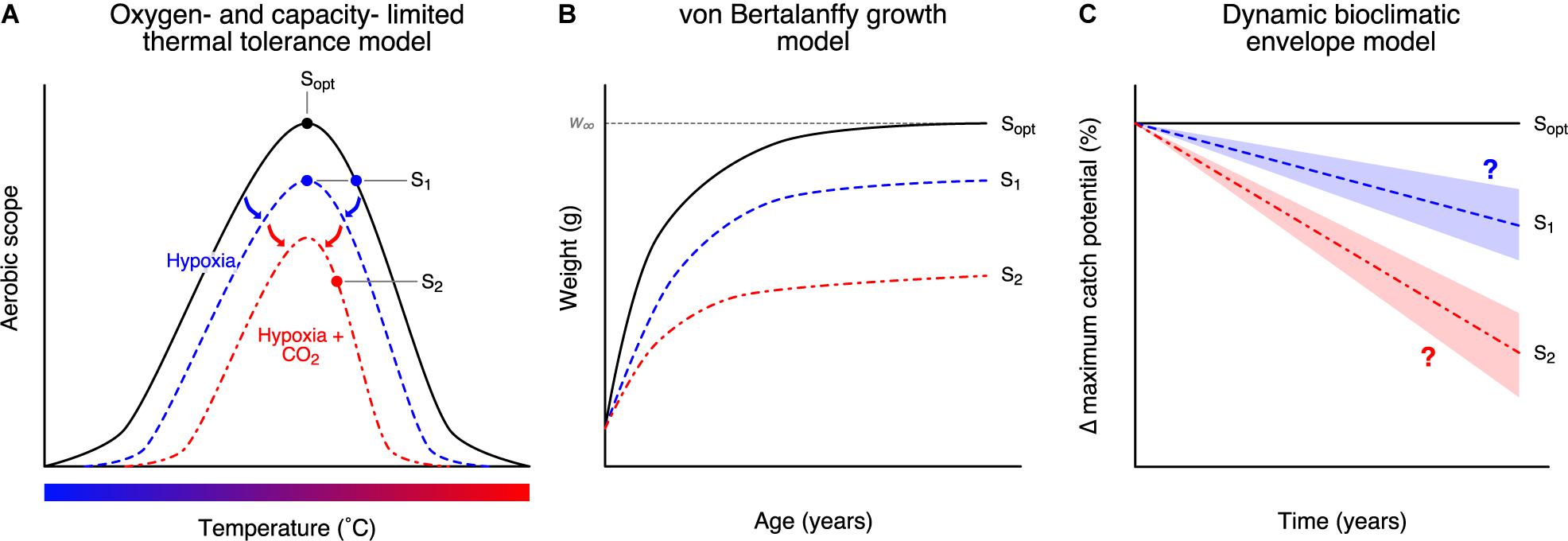
Figure 1. Modelling the pathway of the impacts of ocean acidification from organism to population level in a multi-stressor framework. OA impacts were modelled as (A) physiological impacts (Pörtner and Lannig, 2009), then translated to (B) impacts on growth (Cheung et al., 2011), and (C) impacts on fisheries catch potential (Cheung et al., 2016c). Sopt is the optimal temperature at which aerobic scope is at maximum. Deviations in temperature or other stressors such as hypoxia shrink the overall performance curve (blue curve) and reduce the overall aerobic scope (S1) (A), leading to reductions in growth rate and maximum attainable size (w∞) (B), as well as potential decreases in fisheries catch (C). Multi-stressor impacts of temperature, hypoxia, and elevated acidity will exacerbate physiological limitations and impacts on fisheries catch (red curve; S2).
Understanding the implications of the potential multi-stressor interactions for biological communities and fisheries resources at regional and global scales is important for informing climate change mitigation and adaptation policies. Here, we used a dynamic bioclimatic envelope model to project direct physiological impacts of changes in pH, temperature, and oxygen content on the spatial distribution of commercially exploited marine invertebrate populations (i.e., molluscs and crustaceans) (Pörtner and Lannig, 2009; Cheung et al., 2011; Pauly and Cheung, 2017) – the group known to be particularly sensitive to OA. Our model integrates the oxygen- and capacity-limited thermal tolerance model (Pörtner and Lannig, 2009; Deutsch et al., 2015) and the gill-oxygen limitation model (Pauly and Cheung, 2017) to determine biological responses to environmental drivers and the downstream effects on fisheries catch potential (Cheung et al., 2011, 2016c; Figure 1). Using these models, we expect that OA will affect aerobic scope and translate to changes in growth and fisheries catch, and vary depending on climate change scenario. We focus on using these specific hypotheses for how OA may interact with other drivers in impacting marine organisms – other potential mechanisms are outlined in the discussion.
Materials and Methods
Dynamic Bioclimatic Envelope Model
Changes in catch potential (described below) of commercially exploited species were estimated using a dynamic bioclimatic envelope model (DBEM) (Cheung et al., 2008b, 2011, 2016b). The DBEM predicts how species abundance will change in space (on a 0.5° longitude by 0.5° latitude grid) and time (annual time steps) using an integrative approach by linking species distribution models (Jones et al., 2012), growth models (Pauly, 1980), physiological models (Pauly, 1981), population dynamics models (Pauly, 1980; Hilborn and Walters, 1992; O’Connor et al., 2007), and macroecological models (Cheung et al., 2008a). Changes in species abundance and catch potential are driven by environmental conditions (e.g., temperature, dissolved oxygen concentration, pH) and habitat (e.g., substrate) (see Cheung et al., 2008a). We used environmental data from Earth system model projections (Dunne et al., 2013) as inputs to drive changes in species abundance. We describe the necessary components of the DBEM below; for a thorough description of the model, see Cheung et al. (2008a, 2011, 2016c).
Initial species distributions were obtained from the Sea Around Us database (Close et al., 2006; Jones et al., 2012; Pauly and Zeller, 2015). Their methods use a sequence of criteria to identify and restrict the habitat of each species on a 0.5° longitude by 0.5° latitude geospatial grid (for a detailed description1). First, species habitats were restricted based on recorded presences in Food and Agriculture Organization of the United Nations (FAO) area(s). Next species habitats were restricted to a north–south latitudinal range within the FAO area(s). An expert reviewed range-limiting polygon was overlaid over the map generated from the previous step. Finally, species-specific parameters [primarily collected from SeaLifeBase (Palomares and Pauly, 2017)] including depth range, habitat preference, and equatorial submergence were used to determine the final distribution map.
Species-specific habitat suitability was characterized by overlaying environmental variables including temperature, salinity, depth, sea-ice, primary production, and dissolved oxygen concentration over the initial species distribution maps. Relative changes in these environmental parameters from initial conditions (i.e., start of the simulation) resulted in changes in habitat suitability. Species were assigned to two depth categories – pelagic or demersal – and environmental conditions were assigned accordingly (sea surface and sea bottom, respectively). Habitat preference was also incorporated to characterize a bioclimatic envelope and habitat preference profile for each species (Cheung et al., 2008b). Carrying capacity – the maximum possible biomass in a spatial cell – is determined using the initial species distribution and is positively correlated with habitat suitability (Cheung et al., 2008b, 2016b). A major assumption of the DBEM is that each cell from the initial species distribution is at carrying capacity. As habitat within each cell changes and becomes more (less) suitable, the carrying capacity will increase (decrease).
Individual growth in the model is represented by the von Bertalanffy growth model with species-specific parameters and is constrained by ecophysiological conditions, specifically oxygen and temperature (Cheung et al., 2011). Populations grow using the logistic growth function (Hilborn and Walters, 1992) and population mortality rates are calculated from an empirical equation from Pauly (1980).
Movement of the organisms at different life stages were represented in the DBEM. Larval dispersal is simulated disperse using advection-diffusion models (Sibert et al., 1999; Cheung et al., 2008b), while net adult diffusion rate is determined by a fuzzy logic model (Cheung et al., 2008b). Animals actively move based on the distance between two geographic cells and their relative dispersal rate (e.g., quicker for large-bodied pelagic species, and slower for small reef-dwelling demersal species). Emigration rates are greater if neighbouring cells have a more favourable habitat, while immigration rates are greater if the present cell is preferable to surrounding neighbour cells.
Annual fisheries maximum catch potential (MCP) for each species was estimated by summing the maximum sustainable yield for each occupied spatial cell. Maximum sustainable yield is assumed to be equal to rKCi/4, where r is the intrinsic rate of population growth and KCi is the carrying capacity (biomass) of a spatial cell i.
Modelling Ocean Acidification Impacts in a Multi-Stressor Framework
We modelled the impacts of OA on species abundance in a multi-stressor framework through somatic growth and mortality rates by combining the oxygen- and capacity-limited tolerance and the gill-oxygen limitation hypothesis (Tai et al., 2018). First, we modelled growth rate dB/dt as a function of oxygen supply (anabolism) and oxygen demand for maintenance metabolism (catabolism) (Cheung et al., 2011):
where B is species biomass, and H and k represent the coefficients for anabolism and catabolism, respectively. Anabolism scales with body weight (W) to the exponent d < 1, while catabolism scales linearly with (W), i.e., b = 1. Values of d typically range from 0.5 to 0.95 across species (Pauly, 1981; Pauly and Cheung, 2017; Tai et al., 2018), but we assume a mid-range value of d = 0.7. Higher values of d lead to increased sensitivity of growth to temperature, while lower values lead to marginal decreases in sensitivity (Pauly and Cheung, 2017; Tai et al., 2018). Therefore, d = 0.7 is a conservative measure to use as a scaling coefficient across all species.
Effects of environmental drivers (i.e., temperature, oxygen concentration, and pH) are modelled to affect both growth rate parameters H and k. First, temperature affects both oxygen supply and demand for metabolism (Pauly and Cheung, 2017) following the Arhennius equation (e−j/T). Next, oxygen availability affects overall aerobic scope, while other physiological drivers (e.g., acidification) affects maintenance metabolism (Cheung et al., 2011):
and
The Arhennius equation constants j1 and j2 (for anabolism and catabolism, respectively) are equal to Ea/R, where Ea and R are the activation energy and Boltzmann constant, respectively. T is the absolute temperature (in Kelvin). Relative changes in oxygen [O2] and hydrogen ion [H+] concentration thus change H and k, respectively. These impacts on growth rate can first be depicted as impacts to aerobic scope (Figure 1A). Coefficients g and h were derived for each species from the maximum weight, von Bertalanffy growth rate parameter, and average environmental temperature reported in the literature (Cheung et al., 2011; Palomares and Pauly, 2017).
With changes in aerobic scope due to environmental stressors, our model predicts changes in life-history parameters including asymptotic weight (W∞) and the von Bertalanffy growth rate parameter K (Figure 1B):
and
Environmentally driven changes in life-history growth parameters will affect the size distribution of the population. We used a size transition matrix to model the probability of growing from one size class to the next, as a function of maximum body size W∞ and the von Bertalanffy growth parameter K (Quinn and Deriso, 1999; Cheung et al., 2008b).
Pauly’s (1980) empirical model was used to estimate natural population mortality rates (M):
using maximum body size, growth rate, and the average water temperature of a species range in degrees Celsius (T′). This model was chosen as it is widely used and life-history data is readily available for all of the invertebrate species tested here (Tai et al., 2018). Mortality is then incorporated into the population dynamics logistic growth model, where population abundance (A) decreases (M × A) as a function of the mortality rate.
We modelled OA impacts on survival rates using a correlative approach for both larvae and adults. We measure changes in acidity and its impacts on growth and survival rates as hydrogen ion concentration [H+]. We model changes in life-history traits based on the model:
Surv is the survival rate per year and used here as an example but is also applied to growth. Survival rate in year t is equal to the initial (init) survival rate and the relative change in [H+] between year t and initial [H+] conditions. We define Per as the value of the OA effect size (from Kroeker et al., 2013) for the percent change in survival rate with a doubling of [H+] (Supplementary Table 1). We assume a linear relationship because it is the most parsimonious assumption considering the highly variable responses across species (Ries et al., 2009; Tai et al., 2018). We assume that sensitivities of the organisms reported in Kroeker et al. (2013) represents the mean responses of the studied species in our model’s time-step (annual). OA effect sizes for both growth and survival were assigned based on taxonomic groups for crustaceans and molluscs (Supplementary Table 1). Thus, environmental changes will lead to changes in growth rate, maximum body size, and survival rates. We used the DBEM to scale up and determine how the physiological responses to OA and other environmental drivers affect species distributions and fisheries catch potential (Figure 1).
Modelled Species
We modelled the impacts of OA and climate change on 210 commercially exploited marine invertebrate species. Invertebrate species tend to be more sensitive to OA and changes in pH (Kroeker et al., 2013), while the effects on finfish species are generally less sensitive and show greater variation. We included species from the major shellfish fisheries groups including crabs, lobsters, shrimp and prawns, oysters, scallops, and squid. Most species are distributed throughout coastal waters.
Projections of Ocean Conditions
Projections of changing ocean conditions that drived the biological responses represented by the DBEM from 1950 to 2100 were obtained from Earth system models available from the Coupled Model Intercomparison Project Phase 5 (CMIP5). Specifically, we used outputs from three Earth system models: NOAA’s Geophysical Fluid Dynamics Laboratory 2M (GFDL-ESM); Max Planck Institute for Meteorology ESM-MR (MPI-ESM); and Institute Pierre Simon Laplace Climate Modelling Centre ESM-CM5-MR (IPSL-ESM). We make use of one single realization of each model. All model data were re-gridded onto a 1° × 1° grid, and subsequently interpolated onto 0.5° × 0.5° grid of the world ocean using bilinear interpolation method. Ocean condition variables that were used in the DBEM simulations included sea surface and bottom temperature, pH, oxygen level, salinity as well as sea ice extent, and surface advection. We used annual means for environmental data with 24 time steps per year. Our simulations assume that pelagic and demersal species were exposed to sea surface and bottom conditions, respectively.
Model Uncertainties
We quantified the sensitivity of our DBEM results (Cheung et al., 2016a) to three levels of uncertainty: parameter, structural, and scenario uncertainty. Sensitivity to parameter uncertainty was examined by using the upper and lower 95% confidence limits for OA effect sizes on growth and survival rates. Structural uncertainty is defined here as the variance across different earth system models used as input environmental data. We present results from three earth system models that use various socioeconomic scenarios resulting in various levels of atmospheric greenhouse gas concentrations, known as representative concentration pathways (RCPs) to develop scenarios of environmental change. In our analysis, we use a low (RCP 2.6) and a high (RCP 8.5) carbon emissions scenario for DBEM simulations (van Vuuren et al., 2011). The numbers represent radiative forcing values in the year 2100 relative to pre-industrial periods. The low emissions scenario assumes carbon emissions are strongly mitigated and annual global greenhouse gas emissions peaks within a decade but are then substantially reduced. This trajectory is the closest RCP scenario that aligns with targets set with the 2015 “Paris Agreement” from the United Nations Framework Convention on Climate Change Conference of the Parties. The high emissions scenario is our current pathway, where carbon emissions are not curbed and the burning of fossil fuels continues to be the primary source of energy for the industrial sector. With this scenario, minimal efforts are made to reduce carbon emissions or develop green energy sources. We did not assess the scenario uncertainty of the historical period (2005 and prior).
Analysis
Changes to species abundance were calculated as percent changes between initial and final conditions:
where is the mean abundance of a 10 year period. Change in MCP was also calculated using this formula.
Latitudinal centroid LC for each species was calculated by multiplying the abundance of each occupied cell by the latitude Lat of each cell:
The rate of species distribution latitudinal shift was estimated by finding the slope of a linear regression of the latitudinal centroid for each year. The rate of latitudinal shift was converted to kilometers by multiplying the estimated slope by where r = 6378.2, the approximate radius of the earth. This rate was then converted to decadal shifts. This measures the decadal rate at which species are shifting poleward to cooler waters and the “tropicalization” of marine ecosystems.
Species range size for each year was calculated by summing the product of each occupied spatial cell with its average area. Projected percent changes in range size were calculated using the same formulation as Eq. (8), providing a measure of range size contraction or expansion. Correlations between projected changes in range size and abundance of the modelled invertebrates were examined using Pearson Correlation test.
Effects of OA were isolated from effects of other global change drivers by finding the difference in the outputs between simulations run with modelled effects of OA and without OA [change in hydrogen ion concentration is set to zero in Eq. (3)]. OA is expected to amplify responses in aerobic scope and subsequent life-histories, and these effects were isolated to illustrate the separate and additive effects of OA with other critical global change stressors (i.e., ocean warming, decreased oxygen content) (Cheung et al., 2016c). The projected MCP across pelagic and demersal invertebrates were summed and their changes by year 2100 relative to the average of 1951–1960 were reported.
Results
Intermediary non-spatially explicit results show that modelled impacts of ocean warming and acidification show synergistic effects on aerobic scope, reducing aerobic scope by as much as 75% under the high CO2 scenario by the end of the century (Figure 2A). Continuing with this scenario, maximum body size was projected to decrease by as much as 66% (Figure 2B). Ocean acidification had substantial effects, accounting for over 60% of the reduction in aerobic scope and 32% of the decrease in maximum body size. Global invertebrate MCP was projected to decrease by about 12% in the high CO2 scenario due to physiological (e.g., ocean warming and acidification), and habitat constraints (e.g., primary production, habitat suitability), of which ocean acidification accounts for over 3% of this decrease (Figure 2C). Impacts under the low CO2 scenario are considerably lower, where aerobic scope and maximum body size were projected to decrease by 15 and 23%, respectively, while the change in MCP was negligible (Figure 2).
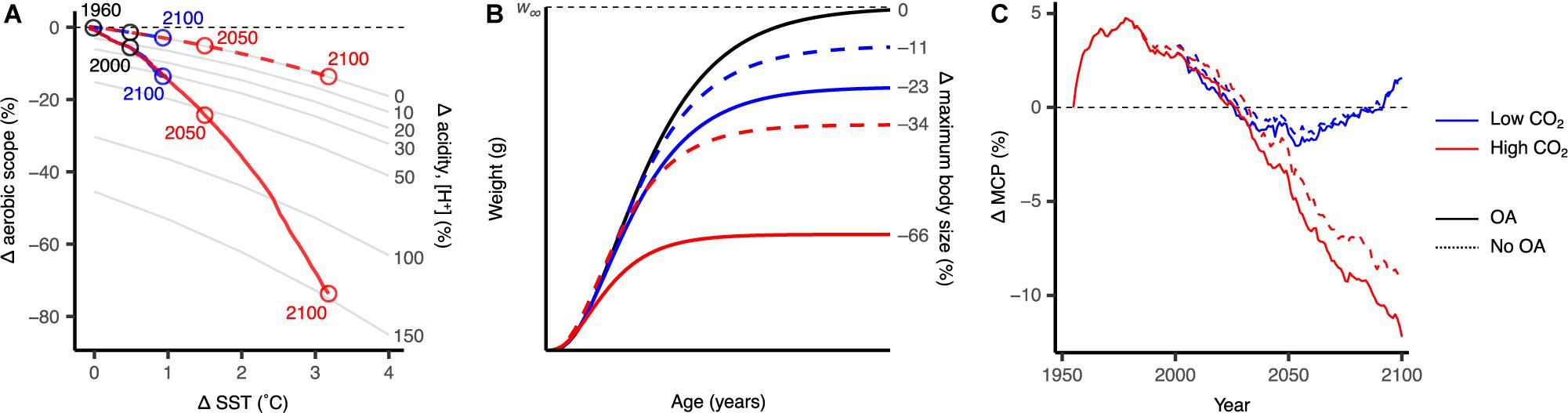
Figure 2. Scaling the multi-stressor responses from the organism level to fisheries catch under the low CO2 and high CO2 climate change scenarios (blue and red, respectively), averaged across all modelled species (N = 210). Differences between projections with and without the modelled effects of ocean acidification (OA) are shown with solid and dashed lines, respectively. (A) Effects of projected ocean warming and acidification on aerobic scope for growth. (B) Change in the von Bertalanffy growth curve and maximum body size in the 2091–2100 period. (C) Changes in global maximum catch potential (MCP) projected by the dynamic bioclimatic envelope model. Results shown are relative to the 1951–1960 period and are multimodel averages from the three earth system models used in this study.
Impacts of global change on the MCP of marine invertebrate fisheries shows regional variation where tropical regions will generally see a loss in catch while northern regions will see an increase if we continue on the “business-as-usual” high CO2 trajectory relative to the strong mitigation low CO2 trajectory (Figure 3). Increases in catch at higher latitudinal regions are largely driven by warming oceans that result in species distribution shifts and increased species turnover (Cheung et al., 2016c). Regions around the coral triangle such as the Indonesian Sea are projected to lose the most (Cheung et al., 2016c), and our models project decreases of >30% for invertebrate catch potential.
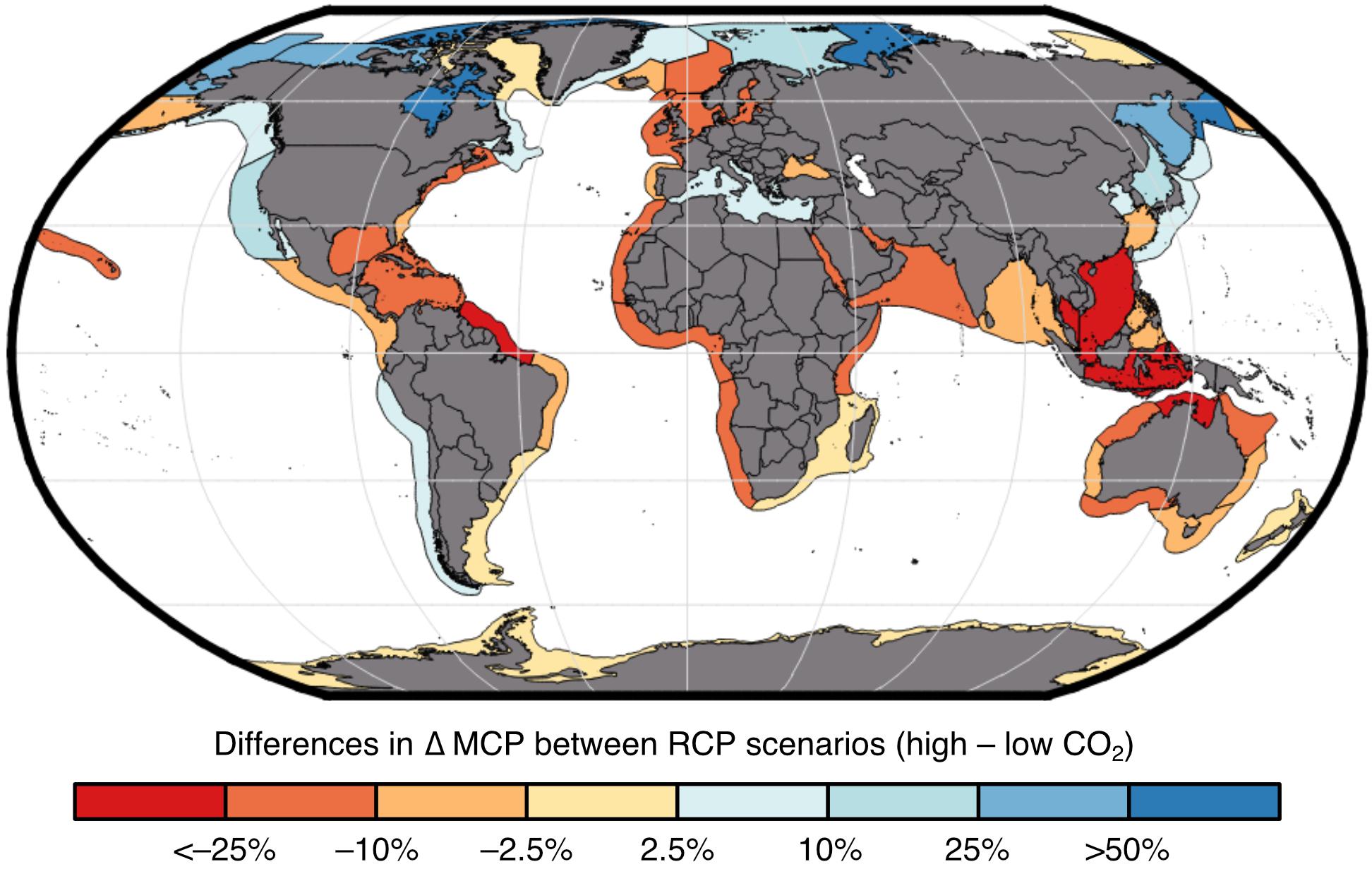
Figure 3. Projected impacts by considering multiple changes in environmental conditions on maximum catch potential (MCP) of marine invertebrates across large marine ecosystems. Results shown are for the 2091–2100 period (relative to 1951–1960) in high CO2 (RCP 8.5) relative to low CO2 scenario (RCP 2.6).
Ocean acidification is projected to decrease annual global invertebrate fisheries MCP by 0.75% for each 0.1 U decrease in surface pH, and 3.4% by the end of the century (Figures 2C, 4A), although this is highly variable across regions. West Arctic large marine ecosystems – including North Bering, Chukchi Sea, Beaufort Sea, Queen Elizabeth Islands archipelago, Canadian high Arctic, and North Greenland – are likely to be most susceptible to OA as pH is projected to decrease by up to 0.5 U and fisheries catch potential to decrease more than 20% by the end of the century in a high CO2 scenario (Figure 4B). While catch potential is projected to increase overall in Arctic regions, OA will largely reduce gains in potential catches for species sensitive to OA (Lam et al., 2014). Our projections show that these impacts due to OA are exacerbated with greater changes in surface temperature and oxygen concentration (i.e., IPSL earth system model) (Figure 4B and Supplementary Figures 1, 2). Currently, there are only a few commercial marine fisheries in the West Arctic (Zeller et al., 2011) – largely restricted by national and international agreements such as commercial fishing bans in the Beaufort Sea and central Arctic – due to our limited knowledge of the baseline state and the sustainability of fisheries exploitation across these regions (e.g., Cobb et al., 2008).
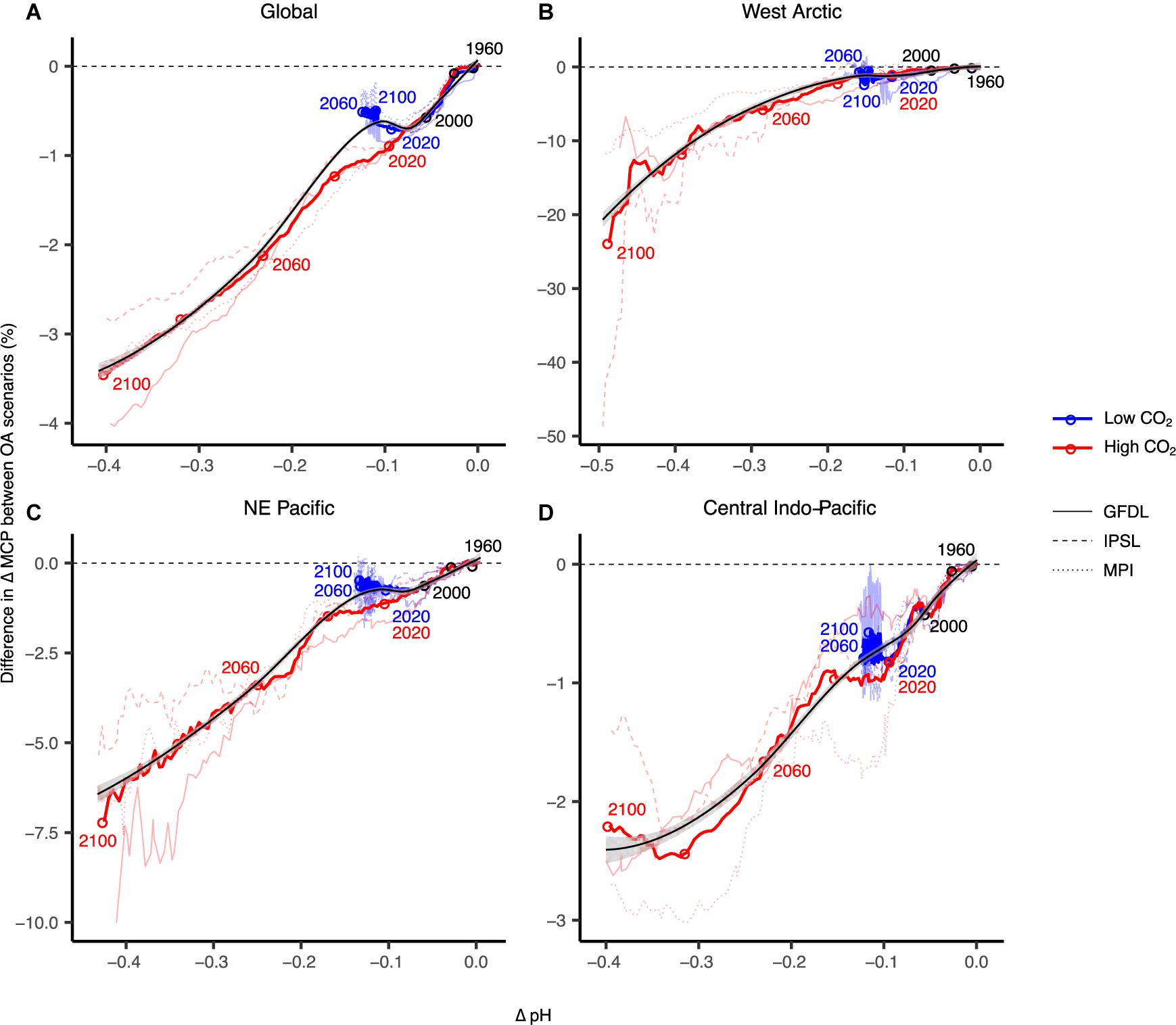
Figure 4. Projected ocean acidification (OA) impacts on maximum catch potential (MCP) of marine invertebrates in addition to other climate change stressors for global (A) and other major regions (B–D). Surface pH is used here to show the relationship between acidity and MCP. Thicker coloured lines are multi-model means and thinner lines are simulations with the different earth system models: GFDL-ESM2M; MPI-ESM-MR; IPSL-CM5A-MR. Black lines and grey bands are selected smoothed regressions and 95% confidence limits. MCP data are smoothed by a 10-year running mean and relative to 1951–1960.
Large marine ecosystems of the Northeast Pacific Ocean show decreases in MCP of up to 6% annually by year 2100 under the high CO2 scenario (Figure 4C). This region includes the highly productive fishing regions of the East Bering Sea, Gulf of Alaska, and California Current large marine ecosystems. Across this region, there are highly valuable capture fisheries including Alaskan king crab and Dungeness crab fisheries, as well as open-system mariculture fisheries such as Pacific oyster and geoduck fisheries (Tai et al., 2017). Other studies using ecosystem models of the Northeast Pacific also found amplified negative impacts on species abundance with multiple global change drivers (Ainsworth et al., 2011). Similarly, projections of OA impacts on the California Current ecosystem showed negative direct impacts on epibenthic invertebrates and downstream indirect impacts on higher trophic level species assemblages (Marshall et al., 2017).
Impacts of OA on fisheries catch potential in the Central Indo-Pacific region (i.e., Gulf of Thailand, South China Sea, Sulu-Celebes Sea, Indonesian Sea) were much less significant, where MCP decreases an additional 2% by year 2100 in the high emissions scenario (Figure 4D). Overall, catch potential across tropical regions is projected to substantially decrease overall due to global change (Cheung et al., 2016c), and while the impacts of OA are negative, they may be overshadowed by temperature-driven changes (McNeil and Sasse, 2016). However, OA effects on critical habitat forming species (e.g., corals, mussels) or key intermediate trophic-level species (e.g., seastars) could lead to substantial ecosystem changes (Hoegh-Guldberg et al., 2007; Sunday et al., 2017).
Biogeographical changes of range size showed a positive correlation (r = 0.78; Supplementary Table 2) with changes in abundance (Figure 5A), while absolute changes in range sizes were positively correlated with increased rates of latitudinal centroid shift (r = 0.52; Supplementary Table 2). For most species, OA had negative impacts on abundance and range size, as well as decreased rates of latitudinal shift (Figure 5B). Species that had large decreases in abundance and range size, quicker rates of latitudinal shift, and exacerbated effects due to OA are likely to be at greatest risk to global change (e.g., banded carpet shell, Atlantic bay scallop) (Figure 5). Such species may also face substantially elevated risk of extinction as population viability is generally positively correlated to range size (Purvis et al., 2000). Some species such as the northern quahog showed positive responses (i.e., range expansion, abundance increase) to global non-OA environmental changes (Figure 5A) and negative responses to OA, likely due to an increase in suitable habitat but limited by the sensitivity to OA. Mollusc species, particularly scallops, mussels and oysters, showed greater losses in catch potential in the high CO2 scenarios when compared with crustacean species (Supplementary Figure 3), explained by the greater effect size for the parameters used for molluscs than crustaceans (Supplementary Table 1). However, changes in catch potential for molluscs showed more variability to the effects of OA, suggesting that the interaction effects of OA and other environmental drivers in our model are not consistent across mollusc species within the same group. Conversely, crustaceans appear to be more robust to OA than molluscs (Ries et al., 2009; Whiteley, 2011; Wittmann and Pörtner, 2013; Kroeker et al., 2013) as they are generally more mobile and thus have the ability to more quickly shift their geographic range.
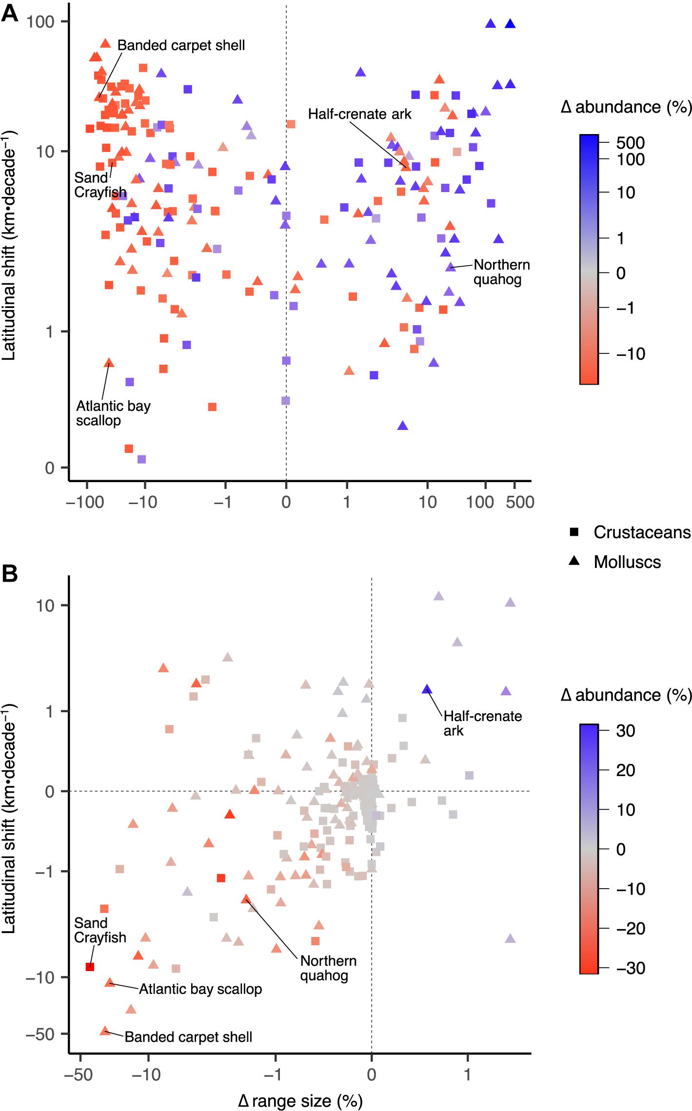
Figure 5. Biogeographical changes in range size, abundance, and distributional shift of latitudinal centroids for 210 invertebrate fisheries species in the high CO2 scenario. (A) Responses to global change drivers excluding ocean acidification, and (B) responses to ocean acidification separated from other stressors. Values shown are multi-model means for 2091–2100 period relative to 1951–1960. Correlations between variables are shown in Supplementary Table 1. Note log scales.
Sensitivity analyses showed that our model results of OA impacts are most sensitive to parameter uncertainty. Parameter uncertainty (OA effect size) accounted for most of the uncertainty (50–90%) in the first half of the model simulations, and decreased to ∼60% in later years (Figure 6). Therefore, it is imperative to obtain accurate empirical data for parameter effect size of OA responses in order to accurately project species responses to global change. This is especially important for more localized and species-specific analyses; our results summarize effects of OA across large spatial extents and many species, therefore we used mean effect sizes across taxonomic groups. Furthermore, the proportion of total uncertainty was smallest for model uncertainty, suggesting our results are robust to the different structures of Earth system models at the global scale. Scenario uncertainty initially accounted for >25% of total uncertainty but its absolute uncertainty was negligible during this early part of the simulation. Scenario uncertainty increased from the year (∼2010) where environmental conditions diverged (Supplementary Figure 2) between low and high CO2 scenarios to account for >30% of the uncertainty by the end of the simulations (Figure 6).
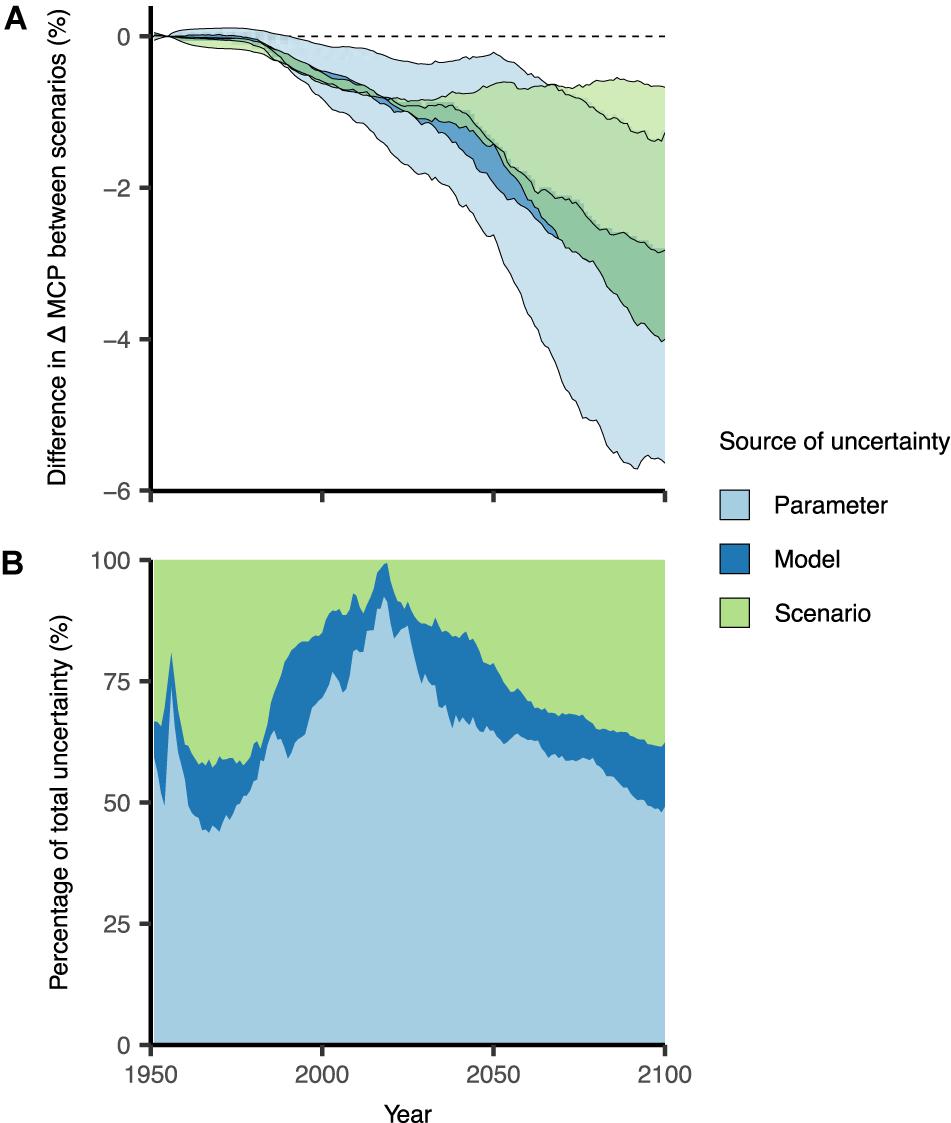
Figure 6. Testing model variability for the projected impacts on maximum catch potential (MCP) due to ocean acidification (OA). (A) Projected changes using the upper and lower bounds of parameter, model, and scenario uncertainty; and (B) the proportion of total uncertainty allocated to each source of uncertainty. Default conditions held constant when testing each source of uncertainty were: (1) parameter = mean OA effect size; (2) model = GFDL-ESM2M; and (3) scenario = RCP 8.5. Results are smoothed by 10-year running means and relative to the 1951–1960 average.
One component of uncertainty not specifically tested here is the various models of mechanistic physiological responses to environmental stressors. The models used here are much less complex than the alternatives (e.g., Then et al., 2015), which generally require a more thorough understanding of the mechanisms involved (Lefevre et al., 2017) and life-history parameters that are not readily available for all species tested. Previous studies have highlighted that the chosen models are not universally applicable (Lefevre et al., 2017; Pörtner et al., 2018), yet the oxygen- and capacity-limited thermal tolerance model provides a connection between physiological constraints and higher ecological phenomena (see response to Jutfelt et al., 2018). Thus, by combining empirical physiological and life-history models, we are able to link environmentally driven changes in aerobic scope to trade-offs with life-history parameters (Tai et al., 2018) – e.g., growth, survival – which then scale to population dynamics.
Discussion
Our current understanding indicates that marine invertebrates are at most risk to the direct effects of OA (Kroeker et al., 2013), although these effects will likely differ across regions (Figure 3). OA effects on marine invertebrate fisheries will have major implications for food security, livelihoods, and the global economy. At over 50 billion USD annually, invertebrate fisheries account for over 1/3 of the value of internationally traded seafood (FAO, 2014). Invertebrates support many valuable fisheries, especially in developing countries where over 50% of internationally traded seafood is caught (FAO, 2014). Developing tropical areas are already projected to be most susceptible to global change (Cheung et al., 2016c) and OA could exacerbate food and income insecurities currently faced in these regions. For example, in areas across the Fijian Islands invertebrates comprise over 70% of artisanal and 50% of subsistence harvests (Teh et al., 2009). Most of the non-subsistence catch in Fiji is exported with the largest invertebrate fisheries valued at $8.4 million FJD (∼$3.8 million USD) in 2003 (Teh et al., 2009). Additionally, small-island developing nations such as the Pacific Islands are highly dependent on invertebrates for both additional income sources and subsistence (Kronen et al., 2010). Ease of access and the minimal gear requirements for invertebrate fishing has facilitated women and even children to participate in subsistence harvesting and remains a source of easily attainable “backup” protein when fishing at sea is unsuccessful (Harper et al., 2013; Codding et al., 2014).
Regionally, invertebrates in the Arctic were projected to be most at risk to ocean acidification, potentially altering the trends in catch potential driven by warming. Previous studies using DBEM projected that ocean warming, reduction in sea ice and increases in primary production increase exploited fishes and invertebrates catch potential in the high latitude regions, although uncertainties of such projections are high partly because of the complexity of changing ocean biogeochemical conditions in the Arctic that were not fully represented in the Earth system models and DBEM (Cheung et al., 2016c). Here, we highlighted that the relatively larger decrease in pH in the Arctic Ocean and its impacts on invertebrates catch potential add to such uncertainties.
For some larger fishing nations invertebrate fisheries make substantial economic contributions. In Canada, lobster fisheries were valued at over $1.1 billion CAD in 2015 and its exports contributed over $2 billion CAD to the Canadian economy (DFO, 2015). Similarly, sea scallops in the United States had dockside revenues estimated at $559 million USD in 2012 (Cooley et al., 2015). Fisheries catch in regions at higher latitudes are projected to increase with global change (Cheung et al., 2016c), but this may not equate to benefits to fishers and the economy. Decreases in highly valuable species (e.g., shellfish) may outweigh any increases in catch of less valuable species, potentially resulting in lost revenues (Lam et al., 2016). If OA has largely negative effects on organism function, this could further reduce overall catch and amplify any losses in fisheries catch. Modelling of OA effects on marine fisheries resources has largely suggested negative impacts to fisheries resources (Ainsworth et al., 2011; Cheung et al., 2011; Lam et al., 2014).
Projection models such as these provide valuable insight for possible future scenarios to identify regions and species that may be most sensitive to global change, and where to concentrate adaptation and mitigation efforts. However, the extent of OA impacts remains uncertain. Impacts of OA on fisheries has been widely discussed and resulted in qualitative and quantitative modelling efforts (Cooley and Doney, 2009; Ainsworth et al., 2011; Ekstrom et al., 2015). These studies are informative and provide a baseline understanding of the potential OA impacts on species and possible downstream effects on fisheries resources. Our spatially explicit, multi-stressor model provides a step toward better understanding how the distribution and abundance of fisheries resources will change at a global scale. Such large-scale models highlight regions that are most susceptible to OA and global change, such as the Arctic (AMAP, 2013), and areas where OA may be overshadowed by other drivers, such as temperature in the tropics (Cheung et al., 2016c). Variability in responses to the different environmental conditions across regions and species indicate which environmental variables are of most concern. Moreover, the global-scale gridded modelled historical environmental conditions that our modelling used do not fully match with local conditions at specific sites as revealed from observations (Bopp et al., 2013). Future studies may apply our modelling framework to local-scale particularly in areas where site-specific data are available. Furthermore, the projected ocean acidification by the Earth system models are more representative of the open ocean where variations in pH are strongly driven by changes in atmospheric carbon dioxide level. However, many exploited invertebrates inhabit coastal areas where ocean acidification is influenced by other non-atmospheric CO2 drivers such as freshwater and nutrient inputs. Future studies could use environmental drivers projected from regional-scale high resolution biogeochemical models which could resolve some of these complexities in factors affecting ocean acidification in coastal waters and their impacts on invertebrates. This could include the incorporation of population-specific estimations of biological sensitivity, if the information is available, to provide finer-grained representations. Then, the capacity of fisheries to adapt and mitigate global change impacts can be evaluated together with biological models to better inform management decisions and conservation efforts. Our study supports previous findings that strong mitigation of CO2 emissions lead to benefits in fisheries catch potential (Cheung et al., 2016c), and that these benefits are further extended due to the minimization of OA. In addition, while our study focuses on the long-term mean trends in the responses of invertebrates to ocean acidification and other environmental drivers, our modelling framework could be applied to study the effects of compounded extremes or environmental variabilities (e.g., marine heatwaves and acidification extremes) on marine species (Cheung and Frölicher, 2020; Ainsworth et al., 2020; Burger et al., 2020).
Accurate projections of OA and global change impacts on marine fisheries require interdisciplinary integration to determine how multiple environmental drivers interact to affect species at various levels of biological organization. Also, previous modelling studies show that ocean warming, deoxygenation and changes in net primary production are important global change drivers on the catch potential and biogeography of marine species with regional variations in their relative importance. Here, we show that adding ocean acidification to these ocean variables further increases the complexity of responses of marine species to multiple environmental drivers under climate change. Thus, development of multi-stressor models requires collaboration between physiologists, biologists, oceanographers, and modellers. The development of modelling impacts of multiple drivers on marine resources is relatively new, yet numerous advances have been made to facilitate efforts and develop a thorough understanding of multi-stressor impacts (Haigh et al., 2015; Koenigstein et al., 2016). Our study contributes to the development of modelling efforts for global change, as well as to better understanding potential interactions of multiple stressors on the spatial distribution of marine fisheries resources.
Data Availability Statement
The raw data supporting the conclusion of this article will be made available by the authors, without undue reservation.
Author Contributions
TT designed and conducted the study. Original model code was written by WC and revised by TT. TT wrote the manuscript with significant contributions from US and WC. All authors reviewed and approved the manuscript.
Funding
This contribution is supported by the Social Sciences and Humanities Research Council (SSHRC) and the Natural Sciences and Engineering Research Council (NSERC) of Canada through partnerships with the OceanCanada partnership and the Marine Environmental Observation Prediction And Response (MEOPAR) Network.
Conflict of Interest
The authors declare that the research was conducted in the absence of any commercial or financial relationships that could be construed as a potential conflict of interest.
The reviewer LK declared a past co-authorship with one of the author WC to the handling editor.
Acknowledgments
WC would also like to acknowledge support from the Nippon Foundation–The University of British Columbia Nereus Program. The content of this manuscript has been published in part as part of the thesis of TT (Tai, 2019).
Supplementary Material
The Supplementary Material for this article can be found online at: https://www.frontiersin.org/articles/10.3389/fmars.2021.596644/full#supplementary-material
Footnotes
References
Ainsworth, C. H., Samhouri, J. F., Busch, D. S., Cheung, W. W. L., Dunne, J., and Okey, T. A. (2011). Potential impacts of climate change on Northeast Pacific marine foodwebs and fisheries. ICES J. Mar. Sci. 68, 1217–1229. doi: 10.1093/icesjms/fsr043
Ainsworth, T. D., Hurd, C. L., Gates, R. D., and Boyd, P. W. (2020). How do we overcome abrupt degradation of marine ecosystems and meet the challenge of heat waves and climate extremes? Glob. Chang. Biol. 26, 343–354. doi: 10.1111/gcb.14901
Alguero-Muniz, M., Alvarez-Fernandez, S., Thor, P., Bach, L. T., Esposito, M., Horn, H. G., et al. (2017). Ocean acidification effects on mesozooplankton community development: results from a long-term mesocosm experiment. PLoS One 12:e0175851. doi: 10.1371/journal.pone.0175851
Bindoff, N. L., Cheung, W. W. L., Kairo, J. G., Arístegui, J., Guinder, V. A., Hallberg, R., et al. (2019). “Changing ocean, marine ecosystems, and dependent communities,” in IPCC Special Report on the Ocean and Cryosphere in a Changing Climate, eds H. O. Pörtner, D. C. Roberts, V. Masson-Delmotte, P. Zhai, M. Tignor, E. Poloczanska, et al. (Geneva: IPCC).
Bopp, L., Resplandy, L., Orr, J. C., Doney, S. C., Dunne, J. P., Gehlen, M., et al. (2013). Multiple stressors of ocean ecosystems in the 21st century: projections with CMIP5 models. Biogeosciences 10, 6225–6245. doi: 10.5194/bg-10-6225-2013
Burger, F. A., John, J. G., and Frölicher, T. L. (2020). Increase in ocean acidity variability and extremes under increasing atmospheric CO 2. Biogeosciences 17, 4633–4662. doi: 10.5194/bg-17-4633-2020
Cheung, W. W., Close, C., Lam, V., Watson, R., and Pauly, D. (2008a). Application of macroecological theory to predict effects of climate change on global fisheries potential. Mar. Ecol. Prog. Ser. 365, 187–197. doi: 10.3354/meps07414
Cheung, W. W., and Frölicher, T. L. (2020). Marine heatwaves exacerbate climate change impacts for fisheries in the northeast Pacific. Sci. Rep. 10:6678.
Cheung, W. W. L., Dunne, J., Sarmiento, J. L., and Pauly, D. (2011). Integrating ecophysiology and plankton dynamics into projected maximum fisheries catch potential under climate change in the Northeast Atlantic. ICES J. Mar. Sci. 68, 1008–1018. doi: 10.1093/icesjms/fsr012
Cheung, W. W. L., Frolicher, T. L., Asch, R. G., Jones, M. C., Pinsky, M. L., Reygondeau, G., et al. (2016a). Building confidence in projections of the responses of living marine resources to climate change. ICES J. Mar. Sci. 73, 1283–1296. doi: 10.1093/icesjms/fsv250
Cheung, W. W. L., Jones, M. C., Reygondeau, G., Stock, C. A., Lam, V. W. Y., and Froelicher, T. (2016b). Structural uncertainty in projecting global fisheries catches under climate change. Ecol. Modell. 325, 57–66. doi: 10.1016/j.ecolmodel.2015.12.018
Cheung, W. W. L., Lam, V. W. Y., and Pauly, D. (2008b). Modelling present and climate-shifted distribution of marine fishes and invertebrates. Fish. Cent. Res. Reports 16:76.
Cheung, W. W. L., Reygondeau, G., and Frölicher, T. L. (2016c). Large benefits to marine fisheries of meeting the 1.5°C global warming target. Science 6319, 1591–1594. doi: 10.1126/science.aag2331
Clark, T. D., and Sandblom, E. (2013). Aerobic scope measurements of fishes in an era of climate change: respirometry, relevance and recommendations. J. Exp. Biol. 216, 2771–2782. doi: 10.1242/jeb.084251
Close, C., Cheung, W., Hodgson, S., Lam, V., Watson, R., and Pauly, D. (2006). Distribution ranges of commercial fishes and invertebrates. Fishes Databases Ecosyst. Fish. Cent. Res. Rep. 14, 27–37.
Cobb, D., Fast, H., Papst, M. H., Rosenberg, D., Rutherford, R., and Sareault, J. E. (2008). Beaufort Sea Large Ocean Management Area: Ecosystem Overview and Assessment Report. Winnipeg, Manitoba.
Codding, B. F., Whitaker, A. R., and Bird, D. W. (2014). global patterns in the exploitation of shellfish global patterns in the. J. Isl. Coast. Archaeol. 9, 145–149. doi: 10.1080/15564894.2014.881939
Cooley, S. R., and Doney, S. C. (2009). Anticipating ocean acidification’s economic consequences for commercial fisheries. Environ. Res. Lett. 4:024007. doi: 10.1088/1748-9326/4/2/024007
Cooley, S. R., Rheuban, J. E., Hart, D. R., Luu, V., Glover, D. M., Hare, J. A., et al. (2015). An integrated assessment model for helping the united states sea scallop (Placopecten magellanicus) fishery plan ahead for ocean acidification and warming. PLoS One 10:e0124145. doi: 10.1371/journal.pone.0124145
Deutsch, C., Ferrel, A., Seibel, B., Pörtner, H. O., and Huey, R. B. (2015). Climate change tightens a metabolic constraint on marine habitats. Science 348, 1132–1135. doi: 10.1126/science.aaa1605
DFO (2015). Fisheries and Oceans Canada National Fisheries Statistics. Available online at: http://www.dfo-mpo.gc.ca/stats/stats-eng.htm (accessed August 28, 2017).
Doney, S. C., Busch, D. S., Cooley, S. R., and Kroeker, K. J. (2020). The impacts of ocean acidification on marine ecosystems and reliant human communities. Annu. Rev. Environ. Resour. 45, 83–112. doi: 10.1146/annurev-environ-012320-083019
Dunne, J. P., John, J. G., Shevliakova, S., Stouffer, R. J., Krasting, J. P., Malyshev, S. L., et al. (2013). GFDL’s ESM2 global coupled climate-carbon earth system models. Part II: Carbon system formulation and baseline simulation characteristics. Am. Meteorol. Soc. 26, 2247–2267. doi: 10.1175/JCLI-D-12-00150.1
Ekstrom, J. A., Suatoni, L., Cooley, S. R., Pendleton, L. H., Waldbusser, G. G., Cinner, J. E., et al. (2015). Vulnerability and adaptation of US shellfisheries to ocean acidification. Nat. Clim. Chang. 5, 207–214. doi: 10.1038/nclimate2508
Fabry, V. J., Seibel, B. A., Feely, R. A., and Orr, J. C. (2008). Impacts of ocean acidification on marine fauna and ecosystem processes. ICES J. Mar. Sci. 65, 414–432. doi: 10.1093/icesjms/fsn048
Furukawa, M., Sato, T., Suzuki, Y., Casareto, B. E., and Hirabayashi, S. (2018). Numerical modelling of physiological and ecological impacts of ocean acidification on coccolithophores. J. Mar. Syst. 182, 12–30. doi: 10.1016/j.jmarsys.2018.02.008
Haigh, R., Ianson, D., Holt, C. A., Neate, H. E., and Edwards, A. M. (2015). Effects of ocean acidification on temperate coastal marine ecosystems and fisheries in the northeast pacific. PLoS One 10:e0117533. doi: 10.1371/journal.pone.0117533
Harper, S., Zeller, D., Hauzer, M., Pauly, D., and Sumaila, U. R. (2013). Women and fisheries: contribution to food security and local economies. Mar. Policy 39, 56–63. doi: 10.1016/j.marpol.2012.10.018
Hilborn, R., and Walters, C. J. (1992). Quantitative Fisheries Stock Assessment. Boston, MA: Springer US, doi: 10.1007/978-1-4615-3598-0
Hoegh-Guldberg, O., Mumby, J., Hooten, J., Steneck, S., Greenfield, P., Gomes, E., et al. (2007). Coral reefs under rapid climate change and ocean acidification. Science 318:1737.
IPCC (2013). in Climate Change 2013: The Physical Science Basis. Contribution of Working Group I to the Fifth Assessment Report of the Intergovernmental Panel on Climate Change, eds T. F. Stocker, D. Qin, G.-K. Plattner, M. Tignor, S. K. Allen, J. Boschung, et al. (Cambridge: Cambridge University Press), doi: 10.1017/CBO9781107415324
Jones, M. C., Dye, S. R., Pinnegar, J. K., Warren, R., and Cheung, W. W. L. (2012). Modelling commercial fish distributions: prediction and assessment using different approaches. Ecol. Modell. 225, 133–145. doi: 10.1016/j.ecolmodel.2011.11.003
Jutfelt, F., Norin, T., Ern, R., Overgaard, J., Wang, T., McKenzie, D. J., et al. (2018). Oxygen- and capacity-limited thermal tolerance: blurring ecology and physiology. J. Exp. Biol. 221:jeb169615. doi: 10.1242/jeb.169615
Koenigstein, S., Mark, F. C., Gößling-Reisemann, S., Reuter, H., and Poertner, H. O. (2016). Modelling climate change impacts on marine fish populations: process-based integration of ocean warming, acidification and other environmental drivers. Fish Fish. 17, 972–1004. doi: 10.1111/faf.12155
Kroeker, K. J., Kordas, R. L., Crim, R., Hendriks, I. E., Ramajo, L., Singh, G. S., et al. (2013). Impacts of ocean acidification on marine organisms: quantifying sensitivities and interaction with warming. Glob. Chang. Biol. 19, 1884–1896. doi: 10.1111/gcb.12179
Kronen, M., Vunisea, A., Magron, F., and McArdle, B. (2010). Socio-economic drivers and indicators for artisanal coastal fisheries in Pacific island countries and territories and their use for fisheries management strategies. Mar. Policy 34, 1135–1143. doi: 10.1016/j.marpol.2010.03.013
Lam, V. W. Y., Cheung, W. W. L., Reygondeau, G., and Sumaila, U. R. (2016). Projected change in global fisheries revenues under climate change. Sci. Rep. 6:32607. doi: 10.1038/srep32607
Lam, V. W. Y., Cheung, W. W. L., and Sumaila, U. R. (2014). Marine capture fisheries in the Arctic: winners or losers under climate change and ocean acidification? Fish Fish. 17, 335–357. doi: 10.1111/faf.12106
Le Quesne, W. J. F., and Pinnegar, J. K. (2012). The potential impacts of ocean acidification: scaling from physiology to fisheries∗. Fish Fish. 13, 333–344. doi: 10.1111/j.1467-2979.2011.00423.x
Lefevre, S., Mckenzie, D. J., and Nilsson, G. E. (2017). Models projecting the fate of fish populations under climate change need to be based on valid physiological mechanisms. Glob. Chang. Biol. 23, 3449–3459. doi: 10.1111/gcb.13652
Marshall, K. N., Kaplan, I. C., Hodgson, E. E., Hermann, A., Busch, D. S., McElhany, P., et al. (2017). Risks of ocean acidification in the California Current food web and fisheries: ecosystem model projections. Glob. Chang. Biol. 23, 1525–1539. doi: 10.1111/gcb.13594
McNeil, B. I., and Sasse, T. P. (2016). Future ocean hypercapnia driven by anthropogenic amplification of the natural CO2 cycle. Nature 529, 383–386. doi: 10.1038/nature16156
Nagelkerken, I., and Connell, S. D. (2015). Global alteration of ocean ecosystem functioning due to increasing human CO2 emissions. Proc. Natl. Acad. Sci.U.S.A. 112, 13272–13277. doi: 10.1073/pnas.1510856112
O’Connor, M. I., Bruno, J. F., Gaines, S. D., Halpern, B. S., Lester, S. E., Kinlan, B. P., et al. (2007). Temperature control of larval dispersal and the implications for marine ecology, evolution, and conservation. Proc. Natl. Acad. Sci. U.S.A. 104, 1266–1271. doi: 10.1073/pnas.0603422104
Palomares, M. L. D., and Pauly, D. (2017). SeaLifeBase. World Wide Web Electron. Publ., Version (06/2017). Available online at: www.sealifebase.org (accessed January 1, 2017).
Pauly, D. (1980). On the interrelationships between natural mortality, growth parameters, and mean environmental temperatuer in 175 fish stocks. ICES J. Mar. Sci. 39, 175–192. doi: 10.1093/icesjms/39.2.175
Pauly, D. (1981). The relationship between gill surface area and growth performance in fish: a generalization of von Bertalanffy’s theory of growth. Berichte Dtsch. Wissenschaftlichen Kommission für Meeresforsch. 28, 251–282.
Pauly, D., and Cheung, W. W. L. (2017). Sound physiological knowledge and principles in modeling shrinking of fishes under climate change. Glob. Chang. Biol. 24, e15–e26. doi: 10.1111/gcb.13831
Pörtner, H. O., and Farrell, A. P. (2008). Physiology and climate change. Science 322, 690–692. doi: 10.1126/science.1163156
Pörtner, H. O., and Lannig, G. (2009). “Oxygen and capacity limited thermal tolerance,” in Fish Physiology, eds J. G. Richards, A. P. Farrell, and C. J. Brauner (Burlington: Elsevier Inc), 143–191. doi: 10.1016/S1546-5098(08)00004-6
Pörtner, H.-O., Bock, C., and Mark, F. C. (2018). Oxygen- and capacity-limited thermal tolerance: blurring ecology and physiology. J. Exp. Biol. 221, jeb169615. doi: 10.1242/jeb.169615
Purvis, A., Gittleman, J. L., Cowlishaw, G., and Mace, G. M. (2000). Predicting extinction risk in declining species. Proc. R. Soc. B Biol. Sci. 267, 1947–1952. doi: 10.1098/rspb.2000.1234
Quinn, T. J. II, and Deriso, R. B. (1999). Quantitative Fish Dynamics. (New York, NY: Oxford University Press). doi: 10.1007/s13398-014-0173-7.2.
Ries, J. B., Cohen, A. L., and Mccorkle, D. C. (2009). Marine calcifiers exhibit mixed responses to CO2-induced ocean acidification. Geology 37, 1131–1134. doi: 10.1130/G30210A.1
Sibert, J. R., Hampton, J., Fournier, D. A., and Bills, P. J. (1999). An advection-diffusion-reaction model for the estimation of fish movement par. Can. J. Fish. Aquat. Sci. 56, 925–938. doi: 10.1139/f99-017
Sunday, J. M., Fabricius, K. E., Kroeker, K. J., Anderson, K. M., Brown, N. E., Barry, J. P., et al. (2017). Ocean acidification can mediate biodiversity shifts by changing biogenic habitat. Nat. Clim. Chang. 1, 81–85. doi: 10.1038/nclimate3161
Tai, T. C. (2019). Building Tools to Model the Effects of Ocean Acidification and How it Scales From Physiology to Fisheries. Ph.D. Thesis. Vancouver CA: University of British Columbia, 226.
Tai, T. C., Cashion, T., Lam, V. W. Y., Swartz, W., and Sumaila, U. R. (2017). Ex-vessel fish price database: disaggregating prices for low-priced species from reduction fisheries. Front. Mar. Sci. 4:363. doi: 10.3389/fmars.2017.00363
Tai, T. C., Harley, C. D. G., and Cheung, W. W. L. (2018). Comparing model parameterizations of the biophysical impacts of ocean acidification to identify limitations and uncertainties. Ecol. Modell. 385, 1–11. doi: 10.1016/j.ecolmodel.2018.07.007
Teh, L. C. L., Teh, L. S. L., Starkhouse, B., and Rashid Sumaila, U. (2009). An overview of socio-economic and ecological perspectives of Fiji’s inshore reef fisheries. Mar. Policy 33, 807–817. doi: 10.1016/j.marpol.2009.03.001
Then, A. Y., Hoenig, J. M., Hall, N. G., and Hewitt, D. A. (2015). Evaluating the predictive performance of empirical estimators of natural mortality rate using information on over 200 fish species. ICES J. Mar. Sci. 72, 82–92. doi: 10.1093/icesjms/fsu136
van Vuuren, D. P., Edmonds, J., Kainuma, M., Riahi, K., Thomson, A., Hibbard, K., et al. (2011). The representative concentration pathways: an overview. Clim. Change 109, 5–31. doi: 10.1007/s10584-011-0148-z
Wahl, M., Saderne, V., and Sawall, Y. (2016). How good are we at assessing the impact of ocean acidification in coastal systems? Limitations, omissions and strengths of commonly used experimental approaches with special emphasis on the neglected role of fluctuations. Mar. Freshwater Res. 67, 25–36. doi: 10.1071/mf14154
Whiteley, N. M. (2011). Physiological and ecological responses of crustaceans to ocean acidification. Mar. Ecol. Prog. Ser. 430, 257–271. doi: 10.3354/meps09185
Wittmann, A. C., and Pörtner, H. O. (2013). Sensitivities of extant animal taxa to ocean acidification. Nat. Clim. Chang. 3, 995–1001. doi: 10.1038/nclimate1982
Keywords: multi-stressor, range shift, climate change, shellfish, fisheries catch, future scenarios, modelling, interdisciplinary primary research article
Citation: Tai TC, Sumaila UR and Cheung WWL (2021) Ocean Acidification Amplifies Multi-Stressor Impacts on Global Marine Invertebrate Fisheries. Front. Mar. Sci. 8:596644. doi: 10.3389/fmars.2021.596644
Received: 19 August 2020; Accepted: 10 June 2021;
Published: 07 July 2021.
Edited by:
Nina Bednarsek, Southern California Coastal Water Research Project, United StatesReviewed by:
Lester Kwiatkowski, UMR 8539 Laboratoire de Météorologie Dynamique (LMD), FranceKirk N. Sato, University of Washington, United States
Victor M. Aguilera, Universidad Católica del Norte, Chile
Copyright © 2021 Tai, Sumaila and Cheung. This is an open-access article distributed under the terms of the Creative Commons Attribution License (CC BY). The use, distribution or reproduction in other forums is permitted, provided the original author(s) and the copyright owner(s) are credited and that the original publication in this journal is cited, in accordance with accepted academic practice. No use, distribution or reproduction is permitted which does not comply with these terms.
*Correspondence: Travis C. Tai, dHRhaTJAYWx1bW5pLnV3by5jYQ==