 Caren Barceló1*†
 Richard D. Brodeur2
 Lorenzo Ciannelli1Elizabeth A. Daly3
 Craig M. Risien1
 Gonzalo S. Saldías4
 Jameal F. Samhouri5
- 1College of Earth, Ocean, and Atmospheric Sciences, Oregon State University, Corvallis, OR, United States
- 2Fish Ecology Division, Northwest Fisheries Science Center, National Oceanic and Atmospheric Administration, Newport, OR, United States
- 3Cooperative Institute of Marine Resource Studies, Oregon State University, Newport, OR, United States
- 4Departamento de Física, Facultad de Ciencias, Universidad del Bío-Bío, Concepción, Chile
- 5Conservation Biology Division, Northwest Fisheries Science Center, National Marine Fisheries Service, National Oceanic and Atmospheric Administration, Seattle, WA, United States
The vast spatial extent of the ocean presents a major challenge for monitoring changes in marine biodiversity and connecting those changes to management practices. Remote-sensing offers promise for overcoming this problem in a cost-effective, tractable way, but requires interdisciplinary expertise to identify robust approaches. In this study, we use generalized additive mixed models to evaluate the relationship between an epipelagic fish community in the Northeastern Pacific Ocean and oceanographic predictor variables, quantified in situ as well as via remote-sensing. We demonstrate the utility of using MODIS Rrs555 fields at monthly and interannual timescales to better understand how freshwater input into the Northern California Current region affects higher trophic level biology. These relationships also allow us to identify a gradient in community composition characteristic of warmer, offshore areas and cooler, nearshore areas over the period 2003–2012, and predict community characteristics outside of sampled species data from 2013 to 2015. These spatial maps therefore represent a new, temporally and spatially explicit index of community differences, potentially useful for filling gaps in regional ecosystem status reports and is germane to the broader ecosystem-based fisheries management context.
Introduction
Major initiatives worldwide have recognized the importance of measuring diversity and community structure as indicators of ecosystem condition (Skidmore and Pettorelli, 2015). Satellite-based remote sensing (RS) is a tool that provides habitat information across large extents at high spatial and temporal resolutions, having the potential to describe the distribution of multiple facets of biodiversity, including species distributions, alpha diversity, predator-prey overlap, and community composition (Skidmore and Pettorelli, 2015; Pittman, 2017; Wallis et al., 2017; Walters and Scholes, 2017; Muller-Karger et al., 2018). As a greater variety of RS-based oceanographic information becomes increasingly available and accessible, scientists have coupled these data with biological datasets collected in situ to develop knowledge in key areas of seascape ecology research, which are in turn useful for fisheries management and dynamic ocean management (Zwolinski et al., 2011; Hazen et al., 2013; Scales et al., 2017). Three key topic areas of seascape ecology research [i.e., research linking oceanography with landscape ecology (Pittman et al., 2011)] include: (1) a better understanding of how terrestrial landscapes affect adjacent seascape patterns and processes, (2) determining which structural attributes of seascapes (defined in Pittman et al., 2011, as: ‘wholly or partially submerged marine landscapes’) drive biotic assemblages and distribution of biodiversity, and (3) quantifying the impacts of climate change on seascape patterns (Pittman et al., 2011). In this study, we address the first two areas and demonstrate potential applicability of our approach to the third.
Pelagic fish and invertebrate communities are among the most ecologically, culturally, and economically important components of marine ecosystems worldwide (Pikitch et al., 2014). The species we focus on here (salmon, sardines, anchovies, squid and mackerel) are at once the object of dedicated and emerging fisheries and critical links connecting lower and higher trophic levels in the coastal ocean (Pikitch et al., 2014; Szoboszlai et al., 2015). As such, understanding the dynamics of pelagic communities is fundamental to ecosystem-based fisheries management efforts. As in other regions, the pelagic community composition of the California Current Large Marine Ecosystem (CCLME) has varied substantially in response to changes in environmental conditions (Brodeur et al., 2006; Ralston et al., 2015; Peterson et al., 2017; Morgan et al., 2019). One of the major environmental drivers influencing the coastal ocean off Washington, Oregon, and northern California is the input of freshwater from the Columbia River (e.g., Hickey et al., 2005; Henderikx Freitas et al., 2018) and the small coastal rivers along the coast (Mazzini et al., 2014; Saldías et al., 2020). These freshwater outflows are a significant source of nutrients, sediments, organic matter and other constituents for the coastal ocean (Sigleo and Frick, 2007; Goñi et al., 2013). The Columbia River plume has been identified as a crucial environment providing nutrients and enhancing the coastal productivity to sustain the ecosystem during periods of delayed upwelling (Hickey and Banas, 2008; Kudela et al., 2010). Thus, the plume can modulate plankton distribution and the aggregation of zooplankton around plume fronts (e.g., Morgan et al., 2005; Hickey et al., 2010). However, the use of RS data products related to coastal freshwater input in the study of epipelagic community dynamics is very limited.
Moving toward ecosystem-based fisheries management of the CCLME requires consideration of the effects of environmental variability and climate on the biota (Field et al., 2006), including the development and evaluation of ecological indicators that directly and indirectly measure environmental impacts on marine communities (Levin et al., 2009; Samhouri et al., 2014; Thompson et al., 2019). Under current marine management policies, predictions of species and ecosystem distributions are necessary for ongoing integrated ecosystem assessments and indicator development (Hidalgo et al., 2016). Leveraging RS data, predictive statistical models can allow for near real-time and hind-casted distributions of individual species as well as community metrics onto multi-layered RS fields. Innovative methods are being used to couple high-resolution RS data with field survey data via statistical modeling techniques to generate fine-resolution predictive maps (Manderson et al., 2011; Hobday and Hartog, 2014; Thorson et al., 2020). However, research that integrates satellite RS data with species diversity, has largely focused on alpha-diversity metrics (e.g., Pittman et al., 2007; Hazen et al., 2013) and less on other community metrics, such as ordination scores representative of assemblage similarities/dissimilarities. Ultimately, forecasts of individual species distributions and community composition metrics can provide an important foundational layer to be used in marine spatial planning, such as dynamic ocean management (Lewison et al., 2015; Maxwell et al., 2015 and references therein).
In this study, we use a pelagic seascape approach and model the epipelagic fish and macro-invertebrate community structure off the coasts of Oregon and Washington using RS and in situ oceanographic biophysical data. First, we assess the relationships among species across different months and community groups. To understand the relationship between community structure and the environment, we use generalized additive mixed effects models (GAMMs) and couple ordination scores with both local in situ collected environmental data and remotely sensed oceanographic data fields. Using the results of these community seascape models, we construct predictive spatial maps of community composition onto the RS layers as hind-casts and predictions at yearly and seasonal scales. From these community structure prediction maps, we extract time series of predicted community gradients. We propose that by coupling readily available RS data with community metrics, we can predict community species composition in the pelagic marine realm, gaining information that can potentially be of use for dynamic regional ocean management.
Materials and Methods
Survey Specifics
From 1998 to 2012 NOAA’s Northwest Fisheries Science Center’s Fish Ecology Division regularly conducted pelagic surface trawl surveys within the Northern California Current (NCC) epipelagic ecosystem with the primary goal of quantifying the marine survival and habitat associations of juvenile salmonids [Juvenile Salmon and Ocean Ecosystem Survey (JSOES); Brodeur et al., 2005]. These surveys were conducted regularly each year in spring-early summer, and late summer, off the coasts of Oregon and Washington between 44.25 and 48.23°N and −125.61 and −123.97°W (Figure 1A). Here, we analyze survey data collected between 2003 to 2012 in order to synchronize with MODIS data availability. The sampling methodology of these surveys was altered after 2012 with respect to the geographical and temporal extent of sampling, and modifications to the gear, impacting catchability and abundance estimates of certain species (Wainwright et al., 2019). However, while comparable ecosystem data (with similar gear configuration) from 2013 to 2015 were collected, they were not made available to us for this analysis/validation purposes. Approximately, 10 transects consisting of between 6 and 8 stations extend from the nearshore to off the continental shelf (approximately 50 km from shore). Thirty-minute surface tows were conducted at each station with a Nordic 264 rope trawl (Nor’Eastern Trawl Systems, Inc., Bainbridge Island, WA, United States) at a speed over ground of approximately 6 km/h. The length of the trawl is 108 m long with a mouth opening of 30 m × 20 m, and the head rope at approximately 1 m from the surface. The mesh size varies along the length of the rope trawl, ranging between 162.6 cm at the mouth to 8.9 cm at the cod end, which had a 0.8 cm liner inside.
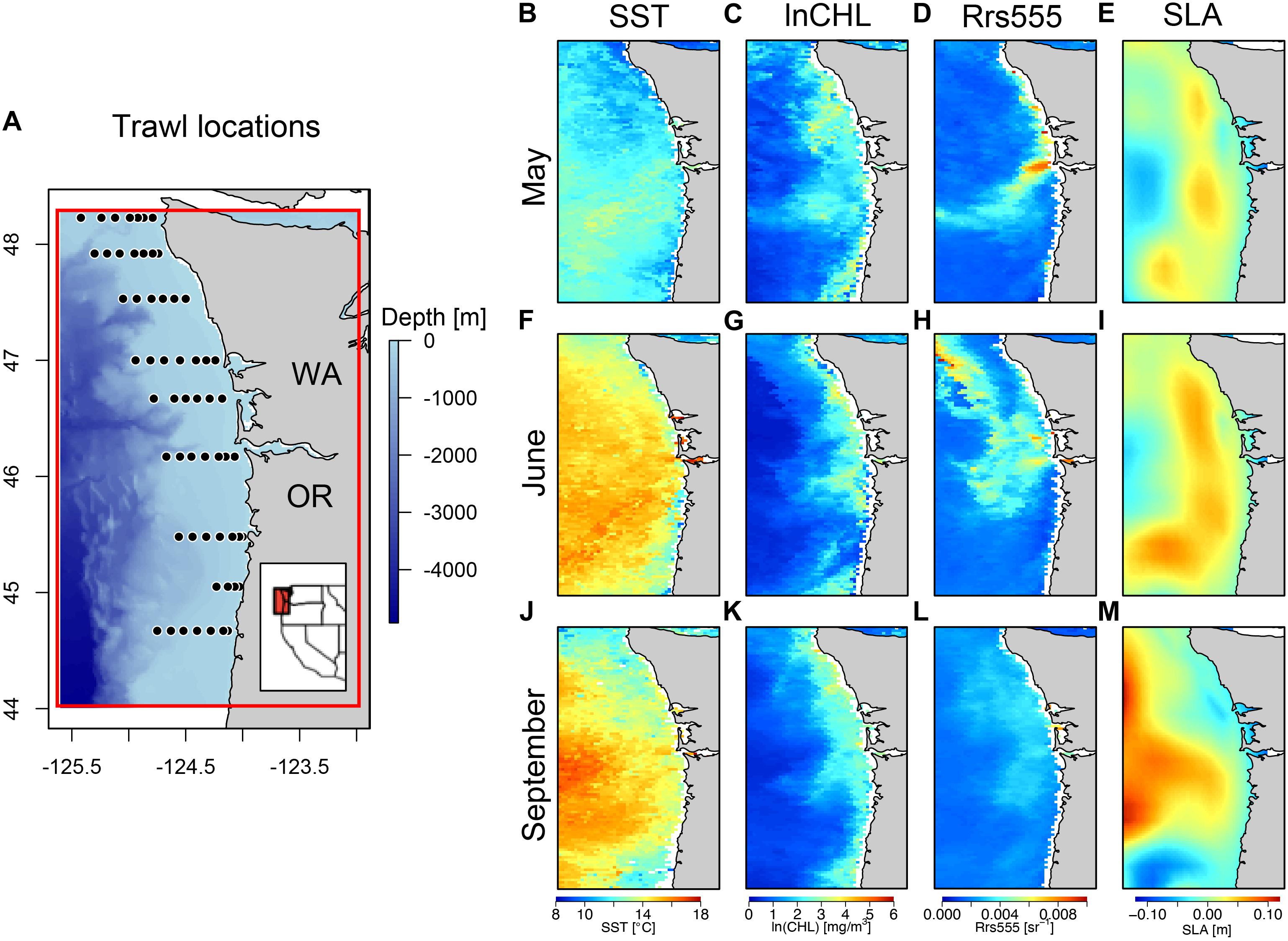
Figure 1. Juvenile salmon and ocean ecosystem survey locations with remotely sensed oceanographic conditions. Locations where survey trawls were conducted off the coast of Oregon and Washington, United States and where in situ oceanographic conditions were measured (not in all years/months) along with images of (A) ETOPO bathymetry (m), (B) MODIS Sea Surface Temperature (SST [°C]), (C) MODIS Chlorophyll-a [mg/m3], (D) MODIS remote sensing reflectance at 555 nm [sr–1], (E) AVISO+TG Sea Level Anomaly [SLA (m)]. (B–E) Example monthly average composites of the remotely sensed data for month of May, (F–I) for June and (J–M) for September of 2006. Red box in inset extent map of the west coast of the United States corresponds to red box surrounding sampling extent in zoomed in bathymetric map.
Species Data
For this study, we restricted the hauls to only those conducted exclusively during daylight hours of the months of May, June, and September. The cruises occurred during the last half of the cruise month, however, on few occasions, some trawls were conducted into the first few days of the next month (into July for example for the June cruise, similarly for May and September). Due to the mesh size used in the trawl, we restricted our community analysis to those species quantitatively retained by the trawl, including both invertebrate and fish species. All species captured in the trawl were identified, counted and measured, with the exception of large catches, where a random sub-sample of fish from each species was measured, counted and weighed and then total abundance re-calculated based on total weight. Catches were standardized by calculating catch-per-unit-effort (CPUE, number per km2) using the distance fished (geographic distance between beginning and end of trawl) (Figure 1A; Daly et al., 2012). Of the total quantitatively sampled species captured between 2003 and 2012 in May, June, and September, we restricted the epipelagic community analysis presented here to species that were found in 3% or more of the sampled stations.
In situ and Remotely Sensed Oceanographic Data
In situ (IS) ocean temperature, salinity, and pressure were recorded at each meter of the water column down to 5 m from the bottom, or to 100 m depth, either prior to or immediately after conducting each surface trawl at a station using a Sea-Bird SBE 19 SeaCAT conductivity/temperature/depth profiler (CTD). At each trawl station (Figure 1A), water samples were collected with a Niskin bottle at a depth of 3 m, and filtered at sea. Pigments were later extracted and analyzed using acetone (90% HPLC grade). Sample fluorescence was measured with a Turner Designs fluorometer (Arar and Collins, 1997). Following Lentz (1992), we calculated mixed layer depth as the depth where the temperature difference relative to the sea surface exceeded 0.02°C.
Moderate Resolution Imaging Spectroradiometer (MODIS) Aqua ocean temperature and multi-spectral color fields for the region off Oregon and Washington were acquired from http://ocean.color.gsfc.nasa.gov/. Specifically, sea surface temperature (SST), chlorophyll-a (CHL), and Remote sensing reflectance at 555 nm (Rrs555) fields were used. SST and satellite derived metrics of primary productivity have been commonly used to define marine habitat for pelagic species as they describe both the thermal conditions as well as potential prey availability (Suryan et al., 2012). Rrs555 fields have been previously used to map the surface expansion of the Columbia River plume throughout the annual cycle (Thomas and Weatherbee, 2006; Mazzini et al., 2015; Saldías et al., 2016) and is likely a good descriptor of community differences due to biological responses to plume-influenced waters (Saldías et al., 2016). All MODIS fields were smoothed using a two-dimensional 3 × 3 grid cell median filter to reduce noise associated with cloud edges and to enhance frontal features in satellite images (Wall et al., 2008; Saldías et al., 2016).
Sea level anomaly (SLA) data were obtained by combining gridded, daily AVISO altimeter fields (Pujol et al., 2016) with low-pass filtered coastal tide gauge data (Risien and Strub, 2016). This 0.25° × 0.25°, blended dataset improves SLA estimates along the coast by removing altimeter data approximately 55–70 km from the coastline and replacing it with a linear interpolation between the tide gauge and remaining offshore altimeter data (Risien and Strub, 2016). In order to have a consistent grid resolution for all RS data fields, we interpolated the blended SLA data to the 4 km MODIS grid using a Barnes objective analysis scheme (Barnes, 1964; Emery and Thomson, 2004). As we were interested in quantifying the distinct water properties associated with distributions of species in the local community, we used both SST and SLA in this study (as done in other species distribution studies, see Becker et al., 2016). SLA and SST are correlated at large scales (Emery et al., 2011) and in the data used here. While MODIS SST is limited to the skin of the sea surface (top 10 microns), SLA is integrative, providing information about the density structure of the water column. As SLA is related to pycnocline depth it may impact habitat quality and availability for distinct species (e.g., a higher SLA is indicative of a deeper pycnocline and therefore potentially more diluted prey availability for pelagic fish and invertebrates, whereas a lower SLA is indicative of a shallower pycnocline which may in turn concentrate prey for pelagic species).
We collocated sampling dates (using actual trawl dates, rather than assigned cruise month) and locations (midpoint of the start and end locations) of surface trawls (Figure 1) with coincident 8-day MODIS and SLA data to the nearest 4 km grid cell for all fields. As we were interested in understanding the fluctuations of the community associated with the regional features (upwelling front, Columbia River plume, eddies) at monthly and interannual time scales, we used 8-day MODIS composites, which McKibben et al. (2012) show to be adequate for comparing IS with RS data off central Oregon. While the sampled species and in situ time series begin in 1998, the time series analyzed here begins in 2003 to allow for the use of consistent RS fields and temporally congruent IS data. Prior to 2003, AVHRR SST and SeaWiFS ocean color data were collected by two distinct satellites with different orbits and timings. The MODIS-Aqua instrument collects SST and ocean color information simultaneously, thus avoiding the issue of mismatched data in time and space. Additionally, SeaWiFS data are only available through mid-December 2010, which does not cover the in situ sampling time series (up to 2012) or the prediction period (up to 2015). To better understand the correlations of IS and collocated RS fields across all stations, all months, and all years, we ran Pearson correlations and report the correlation values (Supplementary Figure 1). In order to create maps of predicted community gradients and to maximize the number of cloud-free grid cells, we created monthly composites of all MODIS and blended SLA fields for the period 2003 to 2012 and predicted community scores onto 3 years (2013–2015) outside of the in situ monthly data collections (2003–2012) (Figures 1B–E). The RS-based oceanographic monthly composited images for the months of May, June, and September between 2003 and 2015 are presented in the Supplemental Information (Supplementary Figures 2–5, respectively).
Community Analysis of the Epipelagic
Non-metric multidimensional scaling (NMDS) ordination (Clarke and Warwick, 2001; McCune and Grace, 2002) using Bray–Curtis dissimilarities was used to quantify the variability in community composition by year and season of the epipelagic juvenile and adult nekton and associated macro-invertebrate community. We specifically chose to use NMDS ordination to quantify the community composition as we do not assume that species are linearly related to each other [a central assumption of principal component analysis (PCAs)/empirical orthogonal functions (EOFs)] (McCune and Grace, 2002).
To explore the spatial changes of the epipelagic nekton and associated macro-invertebrate community by year and season, we performed a NMDS ordination of hauls in species space with a random starting configuration, calculating a dissimilarity matrix using the Bray–Curtis distance measure. The community dataset was composed of 23 relative species abundances (CPUE) by 1215 individual hauls as sample units. The 23 species consisted of salmon, forage fish, and some top predator species, as well as several gelatinous macro-zooplankton and squid representing the macroinvertebrate community. The relative species abundances (CPUE) were log10(x + 1) transformed to reduce the variation between different species abundances. In order to visualize the relationships of in situ and RS data in relation to axes of the NMDS ordination – we used vegan’s envfit (Wood and Scheipl, 2014) function to first obtain a vector overlay on the ordination representing a linear regression of the environmental variables with each NMDS axes. Next, to visualize potential non-linear relationships between each environmental variable and the ordination, we used the ordisurf function that fits a generalized additive model with each variable individually, and produces response surfaces of oceanographic conditions overlaid on the ordination using 2-D thin-plate regression splines. The degree of smoothing is automatically selected by cross validation (Wood and Scheipl, 2014).
We performed a hierarchical cluster analysis to define two community clusters (refer to dendrogram of hauls in Supplementary Figure 6), henceforth referred to as cold and warm communities as they were distributed along the temperature gradient associated with NMDS axis 1. Multiple Response Permutation Procedure (MRPP) was used to determine if the two clusters were significantly different from one another (refer to McCune and Grace, 2002 for a methodological description of MRPP) (A-statistic = 0.056, p < 0.01). MRPP was also conducted by year and month to determine whether these two clusters were significantly different from one another across all years and months (A-statistic range: 0.046 to 0.057, p < 0.01). To assess the exclusivity and fidelity of the species to particular clusters, as well as the statistical significance of the relationship between species abundance and groups of sites in each month, we performed an indicator species analysis (ISA) (McCune and Grace, 2002) on the two groups identified a priori by the hierarchical cluster analysis for each season of data. All non-parametric multivariate statistical analyses were done in R v. 3.4.0 (R Core Team, 2019) using the vegan and indicspecies libraries (Oksanen et al., 2019; R Core Team, 2019; De Caceres and Jansen, 2020).
Relating Community Composition to in situ or Remotely Sensed Oceanographic Data
We used the dimensionless NMDS axis 1 scores from the ordination of hauls in species space as response variables in GAMMs (Zuur et al., 2009) to explore the non-linear effects of oceanographic conditions on the community structure. The GAMM analyses focus on the cold to warm community gradients and how the Columbia River plume affected species communities. We constructed two model set ups, using NMDS axis 1 as the response variables and either in situ and remotely sensed variables as co-variates (i.e., NMDS1∼IS covariates and NMDS1∼RS covariates) (Table 3). We selected the best fit models for each based on minimization of the AIC. All final models and model selection details for NMDS1 are reported in Table 3. Only the community seascape model (NMDS1∼RS) results are discussed here, the other model (NMDS1∼IS) and their resulting functional relationships with environmental co-variates are presented in the Supplemental Information.
Using the linear and non-linear functional relationships of RS environmental data with NMDS axis 1 derived from the GAMM, we predicted the spatial distribution of the response variable (NMDS axis 1) for the different years (2003–2012) and month (May, June, and September) combinations, using monthly composited satellite images. We also used the relationships of NMDS axis 1 to RS covariates, to predict outside the range of the data (2013–2015 in May, June, and September) used here. Spatial predictions were restricted to within the minimum convex hull surrounding the sampled locations.
Generalized additive mixed effects models are a non-linear regression technique where the covariates (environmental variables) are modeled with non-parametric smoothing functions (Hastie and Tibshirani, 1990; Wood, 2015) in the gamm4 library of R (Wood and Scheipl, 2014). GAMMs do not require an a priori assumption of the type of relationship between the covariates and response variables in a model. The environmental co-variates were used as the fixed effects in the models and individual stations as the random effect to account for within station correlation. Variable selection was achieved by minimizing the Akaike information criterion (AIC) as well as the genuine cross validation (gCV) score for each set of models. To calculate gCV, we fit each model to a randomly selected training dataset (with 90% of the total observations), generated predictions for a validation dataset (with the remaining 10% of the observations) and then calculated the prediction error. This procedure was repeated a total of 500 times and a model gCV criterion score was computed by taking the mean squared prediction error (Ciannelli et al., 2007, 2012). The candidate model with the lowest combined AIC (weighted more heavily) and gCV criterion scores was determined to be the best model for determining local IS and RS data relationships with NMDS1.
Results
Oceanographic Correlates With Individual NCC Epipelagic Species
For each species (at stations with positive catch only), we provide the median and range values of remotely sensed oceanographic data (SLA, SST, CHL, Rrs555) in Table 1. The median and range of in situ sampled oceanographic variables (temperature, salinity, density at 10 m depth, and chlorophyll-a (CHL) concentration sampled at 3 m depth), for all 23 species included in this analysis are included in Supplementary Table 1.
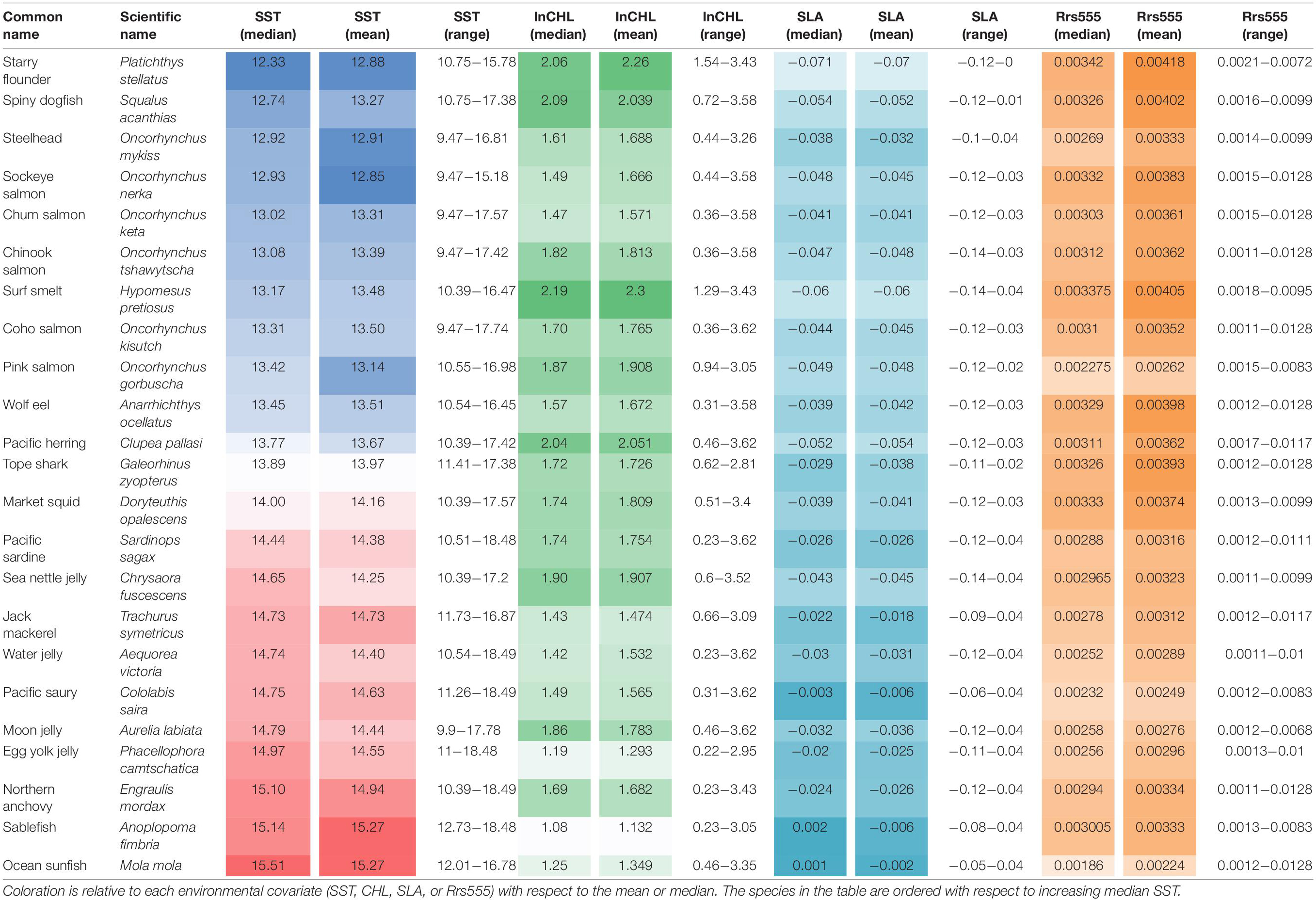
Table 1. Summarized remotely sensed collocated data with positive presence for each species present in more than 3% of the total hauls conducted between 2003 and 2012 during the spring-summer season.
Starry flounder (Platichthys stellatus) followed by surf smelt (Hypomesus pretiosus) were caught most often at the lowest temperatures (median in situ temperature: 10.2, 10.95°C, for each species, respectively), whereas ocean sunfish (Mola mola), followed by sablefish (Anoplopoma fimbria) and then Pacific saury (Cololabis saira), were caught most often at the highest temperatures (median in situ temperature at 10 m depth of 14.2, 13.78, 13.25°C, for each species, respectively). Sablefish (median: 0.657 mg/m3) followed by Pacific saury (median: 0.669 mg/m3) and steelhead (Oncorhynchus mykiss; median: 0.933 mg/m3) were more often caught at stations that had low chlorophyll concentrations, in contrast to starry flounder (median: 1.74 mg/m3) and surf smelt (1.69 mg/m3). Starry flounder was also present in the most saline waters (median salinity: 32.49) followed by pink salmon (O. gorbuscha; median salinity: 32.12), in contrast to steelhead (median salinity: 31.45) and sockeye salmon (O. nerka; median salinity: 31.70). Rrs555 fields were effective at identifying plume vs. non-plume species during sampled months. Specifically, species shown previously to have an affinity for plume waters (Brodeur et al., 2005) including market squid (Doryteuthis opalescens), wolf eel (Anarrhichthys ocellatus), and tope shark (Galeorhinus zyopterus), were captured at relatively high Rrs555 values (>0.003 sr–1). Other species, such as Pacific saury, ocean sunfish, pink salmon, and jellies [including, egg-yolk jelly (Phacellophora camtschatica), moon jelly (Aurelia labiata), and water jelly (Aequorea victoria)], species characteristically associated with the warm community (Brodeur et al., 2005), were captured at relatively low Rrs555 values.
Interannual and Monthly Community Variability
The NMDS 2-D ordination of the survey hauls (1215 total hauls and 23 species) had a final stress of 0.42 (Figures 2A–D). There were significant differences in the communities of fish and macroinvertebrates sampled off Oregon and Washington amongst years (data from months and stations for a given year) (Table 2). However, the degree of differentiation between years was low given the large variability associated with spatial variables and ocean conditions (e.g., Oregon vs. Washington and cold vs. warm conditions) (Figure 2B). The overall yearly MRPP A-statistic was 0.013 (p < 0.05) for year-to-year comparisons when using sample units from the full sampling grid in each month.
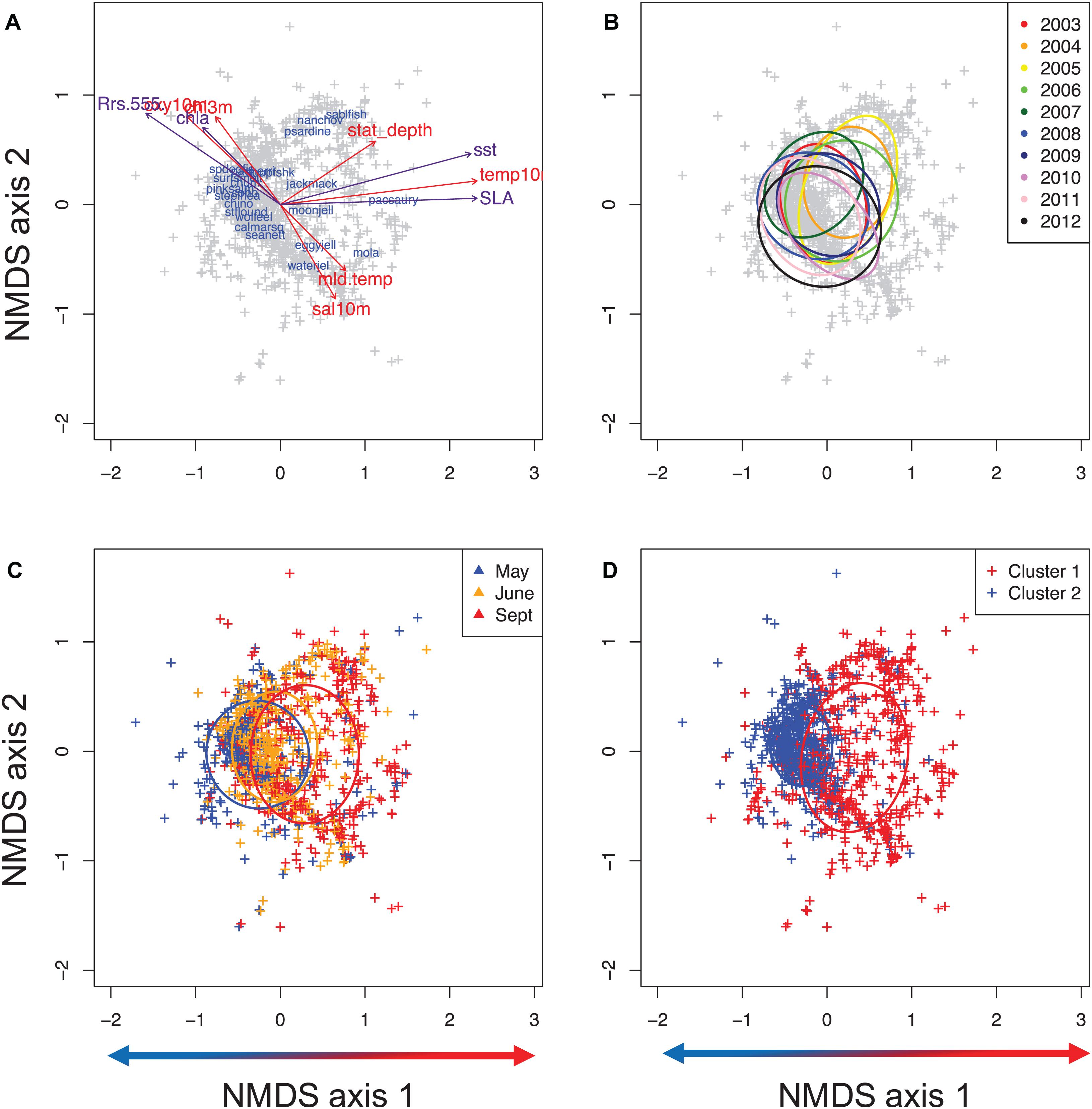
Figure 2. Non-metric Multidimensional Scaling (NMDS) ordination plots of all stations sampled between 2003 and 2012. (A) species centroid overlay with environmental vector overlay, (B) stations colored by year, (C) stations colored by month, (D) Cluster 1: warm vs. cluster 2: cold community clusters. Arrows along axis 1 represent temperature gradient along axes from cold on the left to warm on the right.
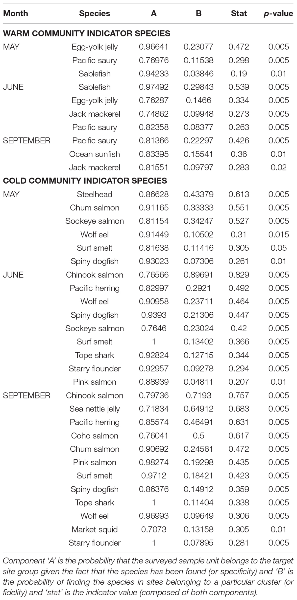
Table 2. Indicator species for both warm and cold community clusters by cruise month.
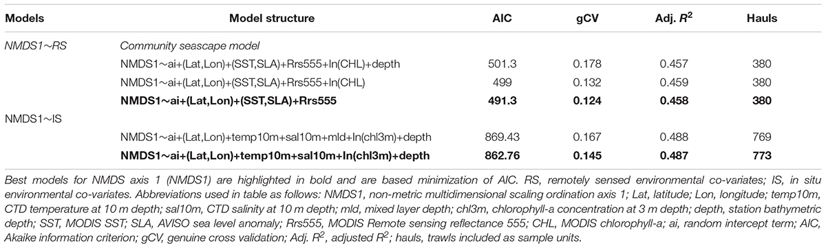
Table 3. Generalized additive mixed model structures and results for models of NMDS axis 1 and NMDS axis 2 with in situ or remotely sensed co-variates and model performance metrics.
Indicator Species of Monthly Community Clusters
Indicator species of monthly communities are presented in Table 2. Pacific saury was the only consistent warm community indicator across all three cruise months. The other warm indicator species differed by month (Table 2). The months of May and June included egg-yolk jelly and sablefish as indicators of the warm community, while in June, Jack mackerel (Trachurus symmetricus) was also an indicator of this warm community cluster. The warm community in September included Pacific saury and Jack mackerel as well as ocean sunfish. The indicator species of the cold community cluster were more variable than those of the warm cluster. The cold cluster indicator species across all months, included salmonids [Chum (O. keta), Chinook (O. tshawytscha), Coho (O. kisutch), Sockeye, Pink salmon], Pacific herring (Clupea pallasii), surf smelt, as well as wolf eel, and Spiny dogfish (Squalus acanthias) (see Table 2). Market squid was a significant cold indicator species in September but not in other months. Steelhead was also found to be an indicator species for the cold community only for the month of May. Species differed by month in their specificity, probability and fidelity to a particular community cluster (Table 2).
In situ Environment Relationships With Community Composition
With respect to the in situ sampled environment, the ordination had a notable cold-warm gradient along NMDS axis 1 and a salinity gradient along NMDS axis 2 (henceforth referred to as NMDS1 and NMDS2). Simple linear regressions indicated that NMDS1 was positively correlated with in situ temperature at 10 m depth and the seafloor depth of the sampling location, which was also partially negatively correlated with NMDS2 (Figure 2A). In situ salinity was positively correlated along NMDS2 while mixed layer depth was positively correlated along both NMDS1 and NMDS2. In situ chlorophyll (at 3 m depth) was negatively correlated with NMDS1 and NMDS2 (Figures 2A, 3A–H). The surfaces of each in situ physical and biological variable overlaid on the NMDS ordination presents the non-linear component of each variable in relation to the community composition (with both NMDS axes) of each haul the ordination (Figures 3A–H). Temperature at 10 m depth had higher temperatures at positive NMDS1 scores and lower temperatures at negative NMDS1, while having both high and low values of temperature at both extremes of NMDS2 (Figures 3A–H). Salinity was more linearly related to NMDS2, indicating a gradient of fresh to warm waters with a positive correlation along NMDS2 (Figures 2A, 3A–H). Chlorophyll had a negative relationship with both NMDS axes (Figure 2A). While oxygen was only sampled from 2006 to 2012, we overlay the non-linear relationship with the community (Figure 3D), but do not use it in the analyses. Communities sampled at shallower stations were concentrated in the upper left quadrant of the ordination (low values of NMDS axis 1 and high NMDS2) whereas communities sampled the deeper water column stations were on the right side of the NMDS ordination (all NMDS2, and NMDS1 values > 0) (Figure 3E). Mixed layer depth largely showed a positive linear relationship with both NMDS axes (Figure 3F). Relationships with latitude, longitude are also presented (Figures 3G,H).
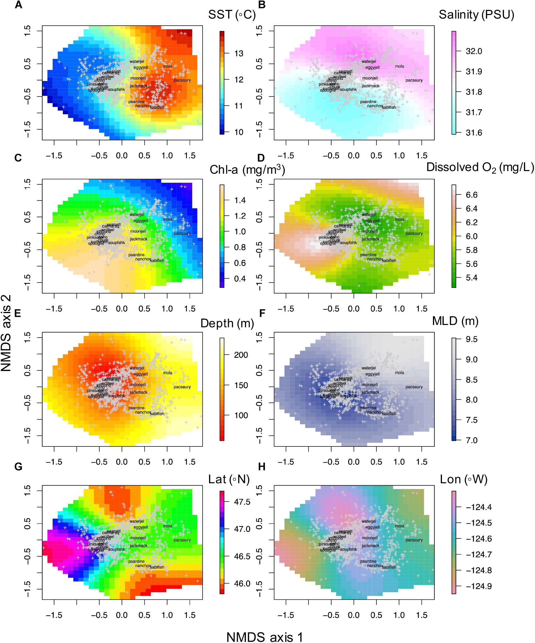
Figure 3. Non-linear relationships of in situ CTD derived oceanographic variables with community structure NMDS axis 1 and axis 2. (A) Temperature at 10 m depth (SST, °C), (B) salinity at 10 m depth (psu), (C) log (chlorophyll at 3 m depth) (mg/m3), (D) dissolved oxygen concentration at 10 m depth (mg/L), (E) station bathymetric depth (m), (F) mixed layer depth (m), (G) latitude (Lat, °N), (H) longitude (Lon, °W).
Remotely Sensed Environment Relationships With Community Composition
The relationships of the RS data fields showed slightly different patterns than the IS data as expected, given the different data sources and depth at which the variables were measured relative to satellite data measurements (see Figures 3, 4). MODIS-Aqua SST had a different pattern compared to the in situ data at 10 m depth. Relatively warm SST (>14°C) ranged between −0.5 to 1.5 values along NMDS1 and along almost the entire NMDS2 (Figure 4A). SST of less than 13°C was restricted to the far-right side of the ordination (NMDS1 values less than −0.5) (Figure 4A). Rrs555 showed a similar pattern to in situ salinity in relation to the ordination, with high values in the lower right quadrant of the NMDS (Figure 4B). MODIS Chl-a demonstrated an almost identical pattern to that observed with in situ Chl-a collected at 3 m depth (Figure 4C).
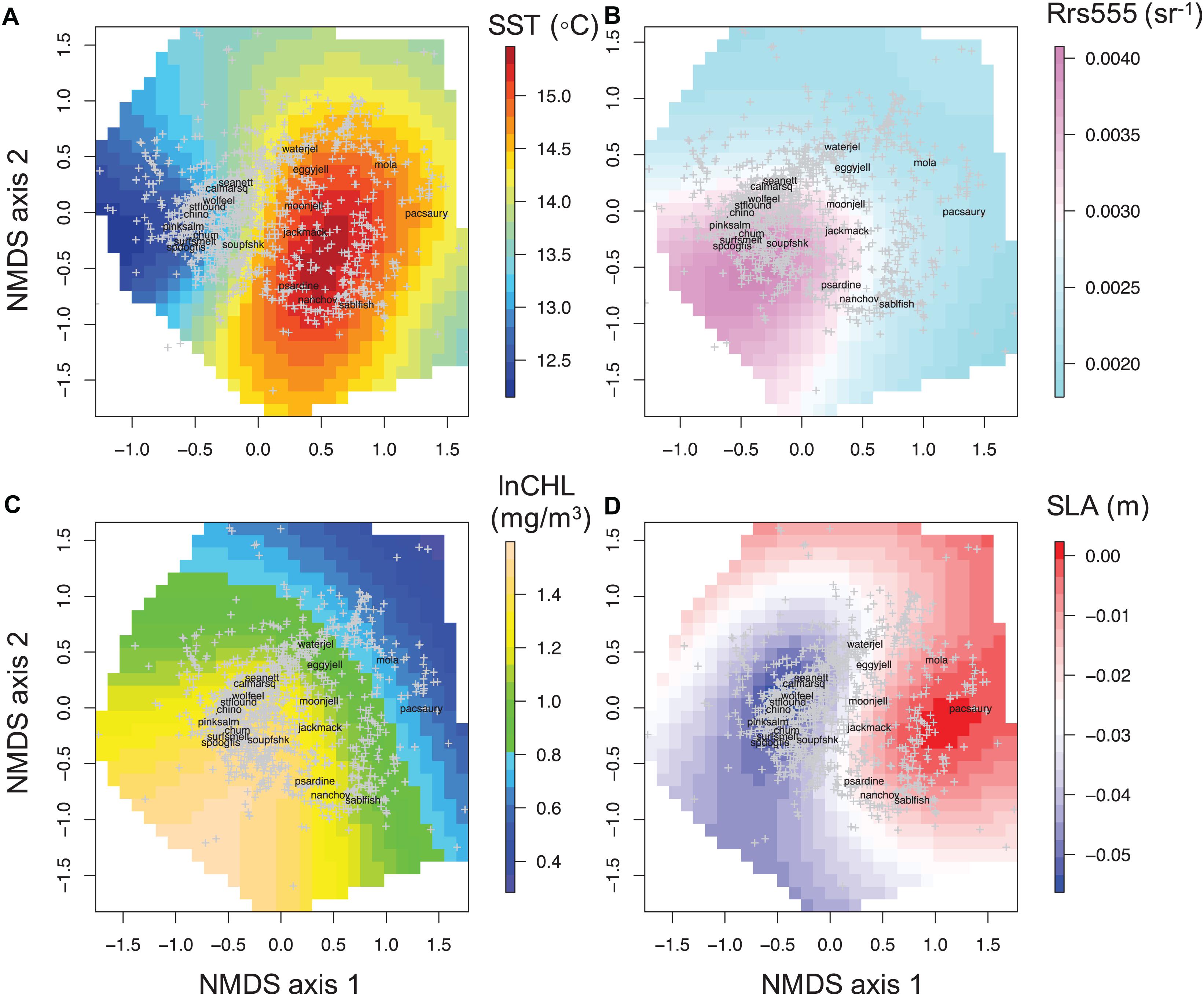
Figure 4. Non-linear relationships of remotely sensed oceanographic variables with the epipelagic Northern California Current community structure. Colors denote a gradient along each environmental variable in two dimensions overlain on the ordination; (A) sea surface temperature; SST (°C), (B) remote sensing reflectance at 555 nm; Rrs555 (sr– 1), (C) log transformed chlorophyll-a concentration; lnCHL (mg/m3), (D) sea level anomaly; SLA (m).
Community Seascape Model Results
The final RS NMDS axis 1 model explained 45.8% of the variability in NMDS axis 1 and included as covariates: (1) an interaction of latitude and longitude, (2) an interaction of SLA, SST, and (3) Rrs555 (Table 3). The average spatial pattern of NMDS axis 1, with low NMDS axis 1 values distributed along most of Washington and higher NMDS axis 1 values distributed off Oregon (Figure 5A). The GAMM interaction biplot of SST and SLA showed a positive relationship of NMDS axis 1 with both SST and SLA (Figure 5B). There was a non-linear relationship of NMDS1 to the Rrs555 data field, with high NMDS1 at low values of Rrs555 (<0.004 sr–1). At Rrs555 values >0.004 sr–1 there was a quasi-linear relationship with negative NMDS axis 1 scores (Figure 5C).
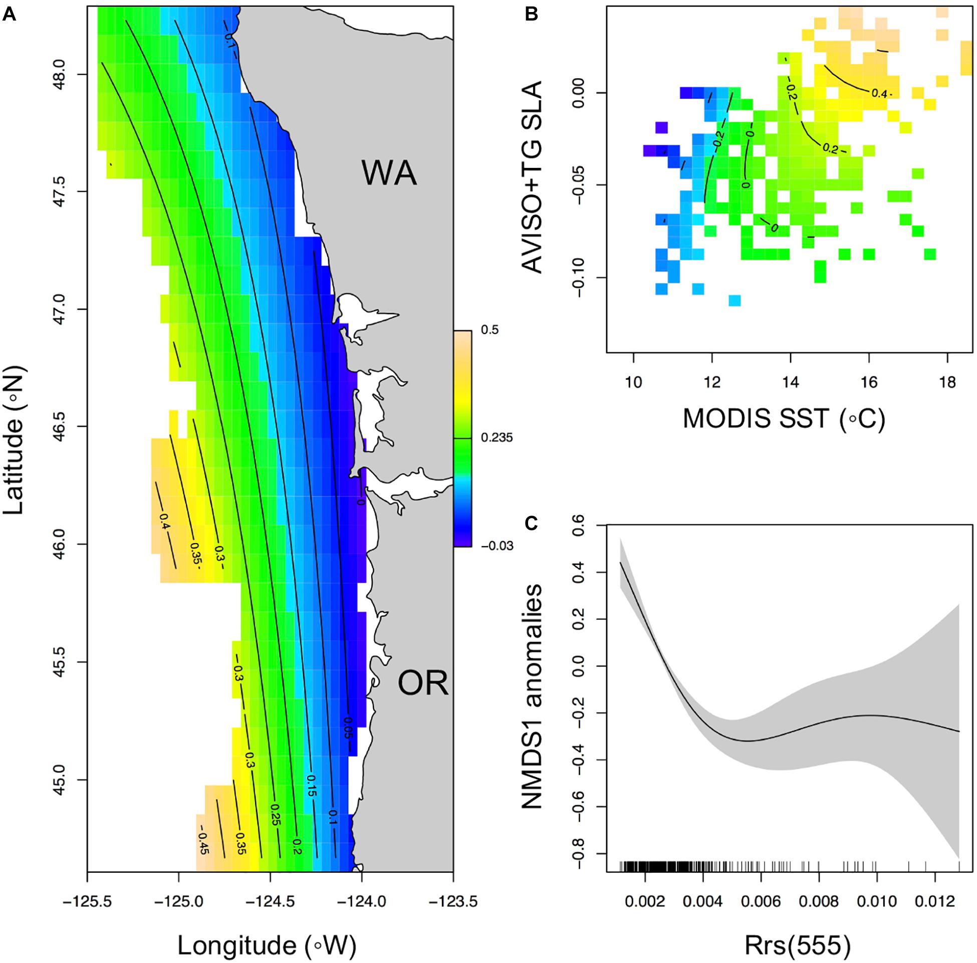
Figure 5. Generalized additive mixed effects model relationships of NMDS axis 1 with significant remotely sensed oceanographic covariates (SST, SLA, and Rrs555). (A) Map of the average spatial distribution of NMDS1 across the sampled time period and area, (B) biplot of the NMDS1 relationship with both SST and SLA, (C) the partial plot of the response of NMDS1 with Rrs555.
Remote Sensing-Based Prediction of Ordination Scores
The best fit NMDS1∼RS model (community seascape model) had significant correlations with the interaction term of latitude and longitude, interaction of MODIS SST with AVISO+TG SLA, and with Rrs555 (Figure 5). Positive values of NMDS1 were generally found offshore, and at higher SST and SLA values and vice-a-versa for negative NMDS1 values. While a formal threshold analysis was not done here, the Rrs555 value where there is no change in NMDS1 occurs at approximately 0.004 sr–1.
Based on the community seascape model (NMDS1∼RS; Figure 5), spatial predictions of NMDS axis 1 values (indicating the gradient from cold to warm communities) indicated differences across years and months (Figure 6). Based on boxplots of extracted predicted NMDS axis 1 values for the Oregon and Washington regions as well as the whole sampled region, Oregon had a higher presence of warm community during all months–years (Figure 7), while Washington had a greater presence of the cold community across all months–years (Figure 5). During some months and years (May 2005, May 2008, June 2008, June 2012, June 2006, September 2006, September 2012, June 2014), the difference between Oregon and Washington was pronounced (Figure 7).
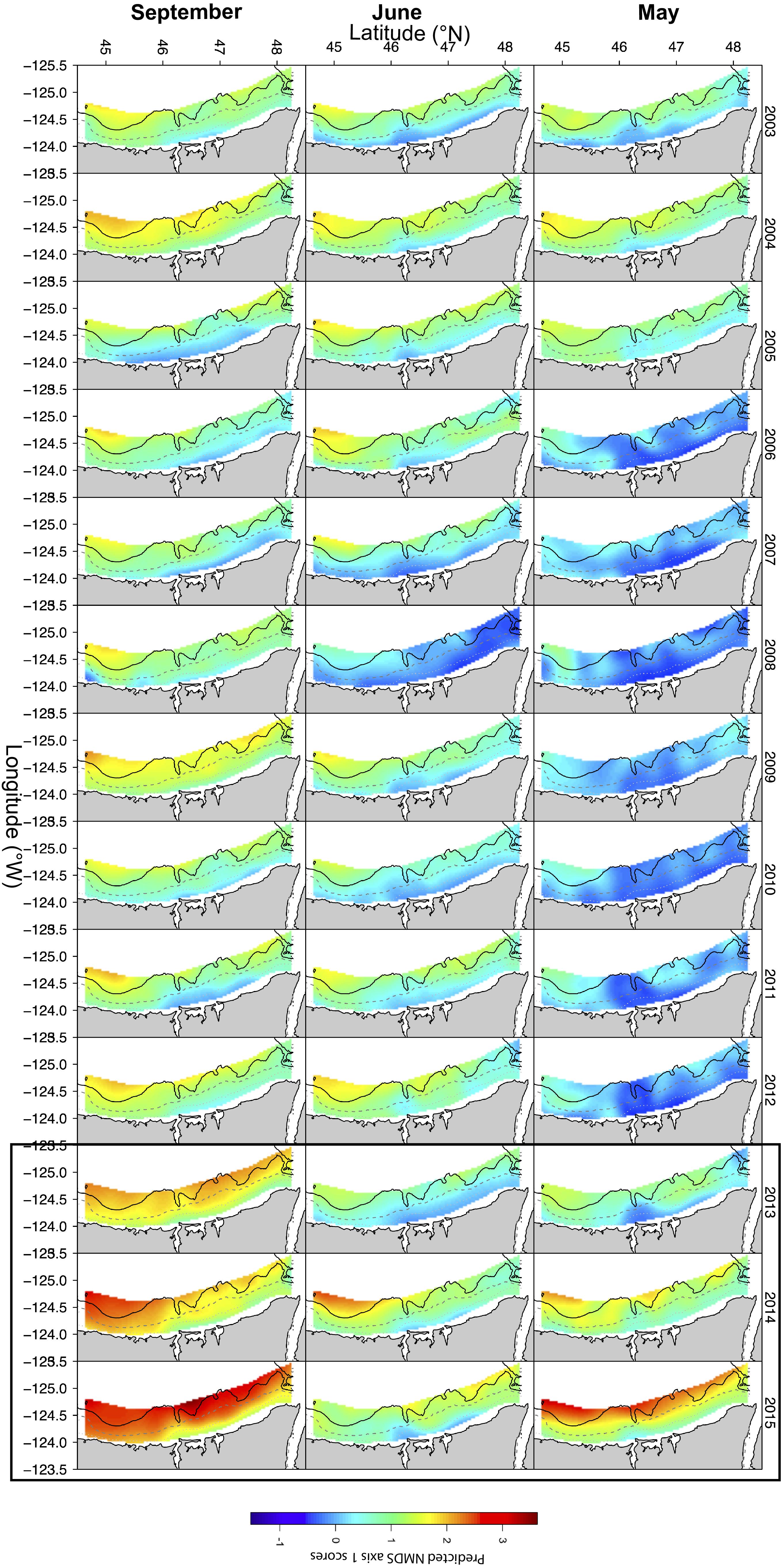
Figure 6. Spatial predictions of NMDS axis 1 (representing the warm to cold-onshore community composition gradient) onto statistically (GAMM) combined remotely sensed MODIS data products in May (top row), June (middle row) and September (bottom row) between 2003 and 2012. May, June and September months of years 2013–2015 are predicted using prior data. Black box surrounding years 2013–2015 encompasses month/years where predictions were made outside of the range of the data included in the GAMMs.
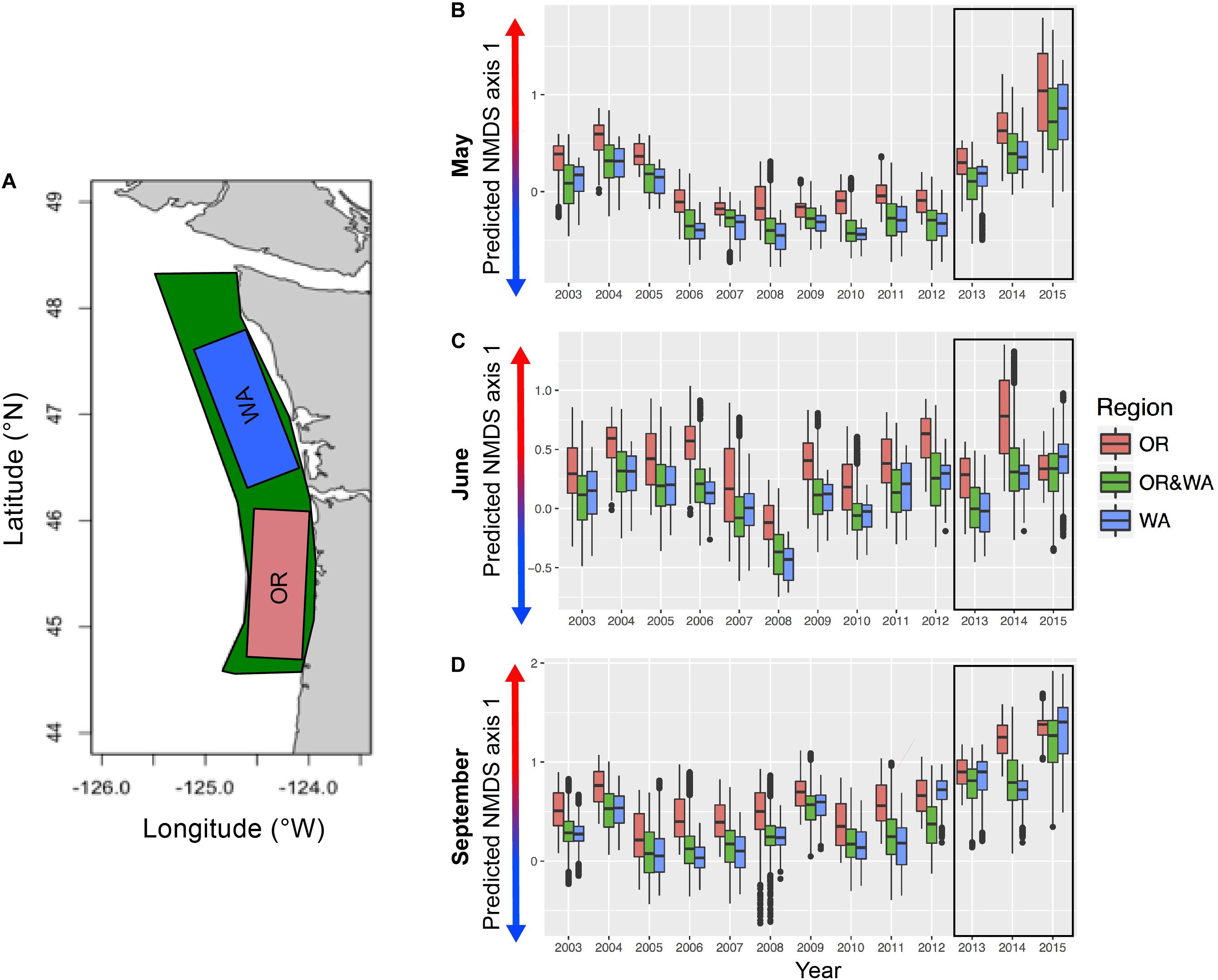
Figure 7. Epipelagic community seascape index. Boxplots of the warm to cold community composition gradient (values plotted in boxplots are NMDS axis 1 scores) in each region [(A) entire area sampled (green), OR (pink) and WA (blue)] during the month of (B) May, (C) June, (D) September. Higher values of NMDS axis 1 represent greater presence of warm community (warmer colors on arrows), lower values of NMDS axis 1 represent greater presence of cold community (cooler colors on arrows). Black box surrounding years 2013–2015 encompasses month/years where predictions were made outside of the range of the data included in the GAMMs.
In May, the period between 2003 and 2005 had a higher presence of the warm community across the entire sampled extent, with a greater presence of the warm community in Oregon than for Washington or the full region (Figure 7). For this month, from 2006 to 2012, there was a lower presence of cold community across the whole region (Figure 7). For May 2013–2015, a significant increase in the presence of the warm community was predicted for all regions, with 2015 having the highest presence of the warm-offshore community within our hind-casted and fore-casted time series. In June, between 2003 and 2005 there was a greater incursion of the warm community than other years (Figure 7). Years with little to no presence of the warm community included 2007 and 2008 (Figures 5, 6). For both Oregon and Washington, September of 2004 and 2009 had the highest predicted warm community presence.
Between 2013 and 2015, for May and September there was a pronounced predicted increase in the presence of the warm-offshore community, especially off Oregon (high positive values of NMDS1). June and September of 2014 both had notably higher predicted presence of the warm community relative to the full area and to the Washington area. For all regions, June 2015 was similar to the long-term mean predicted NMDS1 scores. However, in both May and September, the predicted NMDS1 scores were higher than any previous year and had values greater than the most positive of the observed NMDS1 scores (up to 2012).
Discussion
The field of pelagic seascape ecology so far has dealt mainly with the prediction of species distributions onto RS data fields (e.g., Alvarez-Berastegui et al., 2014, 2016), as well as the long-standing tradition of categorizing ocean waters based on RS data (Jerlov, 1968; Kavanaugh et al., 2014). More recently, predicting individual species distributions onto clustered RS data fields has also been attempted. For example, Breece et al. (2016) classified MODIS ocean color and SST fields, and then predicted Atlantic sturgeon habitat (using acoustic receiver tracked movements of individuals) onto categorized images based on a cluster analysis of multiple RS data fields. Here, we chose a different seascape approach: prediction of community gradients onto RS data by linking ordination axes describing community composition onto statistically amalgamated RS-data fields given the relationships defined by non-linear regressions (GAMMs). The relationships between marine species distributions and the environment are often non-linear (McCune, 2006; Lintz et al., 2011), as are the relationships of gradations in community composition to the environment. Our use of a continuous community gradient response variable (ordination axes) avoids drawbacks associated with classified community clusters, which includes unrealistic crisp borders and potential misclassification of species to distinct clusters (Lintz et al., 2011). It also allows for the description of non-linearities between individual RS data fields and community gradients (e.g., Figures 4A–D). Our approach of using a community metric has been instrumental in uncovering useful ecological information that other approaches could not have revealed. Notably, we found that at the community level, spatial and temporal dynamics are well represented by and correlated with remotely sensed and in situ oceanographic variables, indicating a high degree of spatio-temporal variability of each identified assemblage (e.g., warm–cold) in the NCC.
This is the first study in this region that assesses Rrs555 in relation to the nekton and macro-invertebrate community. MODIS Rrs555 data are known to be related to pelagic biology in this region (Thomas and Weatherbee, 2006; Saldías et al., 2016), but this is the first study in this region to demonstrate the utility of using MODIS Rrs555 fields for biological studies. Furthermore, the species associated with the highest Rrs555 median values are generally understood to be related to the plume or relatively fresh waters, while those with the lowest Rrs555 median values given their distributions during this sampling period are indicators for the ‘warm community’ (Brodeur et al., 2005). In addition, we demonstrate the utility of using the interaction of both SST and SLA, as together they capture the local physical expression of ocean indices such as PDO and the North Pacific Gyre Oscillation in species distribution models, rather than individually or together as additive co-variates (as is often done in species distribution modeling of organisms). SST in this region is at times strongly influenced by the warmer Columbia River plume waters (Saldías et al., 2016) and relatively cool upwelled waters during the spring-summer season. From our correlations of collocated MODIS SST and SLA at sampling locations, SST is positively correlated with SLA, indicating that these variables capture complementary yet distinct aspects of the marine environment (SST is only representative of the surface skin conditions of the ocean and SLA provides a more depth integrative understanding of the surface ocean capturing both density and regional circulation features).
The GAMM models predicted community differences based on RS oceanographic variables, capturing predicted NMDS1 scores outside the range observed during the sampled 10 years during all months. This is likely indicative of a distinct offshore community configuration occurring in the Oregon and Washington shelf and slope waters during the 2014–2015 (variable by season) period, due to anomalously warm water temperatures during 2014–2015 heatwave years (Gentemann et al., 2017; Peterson et al., 2017; Brodeur et al., 2019; Morgan et al., 2019). There are limitations with respect to the inferences we can make about the spatio-temporal community predictions past the extent of our empirical sampled data. That said, our results do suggest an anomalous offshore community in 2014–2015 which agrees with results from other studies in the region and adjacent that analyzed empirical data from that time period (e.g., Brodeur et al., 2019; Morgan et al., 2019). For example, Auth et al. (2018) recently identified novel ichthyoplankton assemblages in this region after 2014, due to the Northeastern Pacific (NEP) marine heatwave of 2014–2016 influencing the early and more coastal spawning of northern anchovy and Pacific sardine, and the more northerly and coastal spawning of Pacific hake (Merluccius productus). In the central California Current System, Santora et al. (2017) identified anomalously high diversity during this 2014–2016 NEP marine heatwave. Our prediction of community composition onto RS-data fields allowed for the spatial distribution of the compositional gradient, and thus has broader ecological implications. Almost all years and months had a significantly lower presence of the warm community along the Washington shelf than off Oregon (Figures 5, 6). This region is similar to that identified by Barceló et al. (2018) as a cold water refugia and provides evidence that the coastal region off southern Washington has a consistent onshore affinity community that is consistent across multiple months during the spring-summer upwelling season.
The two community clusters identified in this study, represent what we describe as the ‘cold community’ or the ‘warm community.’ These communities are represented by pelagic species that have either warm (offshore and/or southern) or cold-water (northern and/or nearshore) affinities (Brodeur et al., 2003). The ‘warm community’ might be further subdivided into a Columbia River plume vs. the warm, but non-plume community (Supplementary Figure 6). However, this separation was not distinguished in this study, and possibly not clearly defined for all months due to the variable spatial extent of the plume as well as the use of the plume by a wide range of both warm and cold affinity, nearshore and offshore species. Northern anchovy and Pacific sardine clustered together with sablefish in the ordination (Figure 2A) in a different region of the ordination than either Pacific saury or ocean sunfish, and are species known to be associated with the Columbia River Plume during the spring-summer upwelling season (Emmett et al., 2004; Litz et al., 2008).
The indicator species in each month for the monthly warm clusters (Table 1) consistently had Pacific saury as an indicator. This species is often captured at offshore stations; however, its schooling behavior leads to a highly variable catch predictability in these stations (Brodeur and Pearcy, 1986; Brodeur et al., 2004, 2005). Sablefish (age-0) was also an indicator of the ‘warm community’ in May and June, but given median values of CTD salinity and Rrs555 it may also be a Columbia River plume associated species (Brodeur and Pearcy, 1986). The ISA indicated that September also included Jack mackerel and ocean sunfish, likely due to an increased presence of warm offshore water along the shelf. With respect to the shared indicator species among the 3 months, May and June shared two of the species, and June and September shared two different species, while all 3 months shared Pacific saury. This is indicative of an expected, compositional continuum (vs. completely different warm communities between May to September) throughout the spring-summer season of makeup of the offshore community composition.
The fluctuation of the warm vs. cold community gradient has implications from a food-web and fisheries perspective. The closer to shore the preferred habitat for species of warm water affinity is, the higher the degree of competition and/or potential habitat compression for colder affinity species (such as juvenile and sub-adult salmonids). This concept is analogous to vertical habitat compression of the mesopelagic community due to the vertical expansion of oxygen minimum zones (Stewart et al., 2014; Checkley et al., 2017), but instead, from a horizontal perspective. A concentrated presence of the cold community into the near-shore implies potentially higher competition among similar trophic level species, leading to reduced success, as well as higher predation by coastal predators (colonial seabirds and pinnipeds), potentially further reducing already low populations of forage fish and salmon species. On the other hand, the near-shore intrusion and increased presence of the offshore community may introduce higher trophic level species (e.g., Santora et al., 2020), such as albacore, making these species more easily available to the fishery (less travel time to fishing grounds for fishers).
Further, community seascape derived indices can add to integrated ecosystem assessments, by filling in gaps in survey coverage (e.g., resulting from global pandemics) and providing information about the state of the ecosystem that can then be used to relate to other trophic levels and human activities. Similar to the cold-water lipid-rich copepod community versus warm-water, lipid-poor copepods in the northeastern Pacific Ocean (Peterson et al., 2017), the warm–cold community gradient metrics described here (Figures 5, 6) have both spatial and temporal qualities. As such, they measure both the ‘flavor’ of the regional community, as well as the spatial presence of different community groups. This metric of warm–cold epipelagic fish fluctuations could be added to the suite of regional biological condition indicators of the upper ocean that have been related to higher trophic levels, such as salmon returns (Burke et al., 2013), or as a predictor for the yearly distribution of albacore habitat for fishermen. This metric also could contribute to the suite of diversity indicators used in the California Current Integrated Ecosystem Assessments as a new, community composition-based indicator of upper ocean ecosystem state. Furthermore, these data and community predictions could be integrated into seasonal forecasting products, such as J-SCOPE1 (Siedlecki et al., 2016; Malick et al., 2020) and extended to use Regional Ocean Model System (ROMS) data to provide useful information on coastal pelagic species’ essential fish habitat.
In this study, we combined analytical techniques for understanding community structure with in situ and RS oceanographic observations to develop a better understanding of the community seascape. This analysis determined the habitat associations and community gradients in this upwelling and river-plume influenced pelagic marine ecosystem. These results demonstrated a statistically significant relationship between in situ and remotely sensed environmental variables and community composition that can have major benefits in monitoring and managing multi-species communities regionally, ranging from zooplankton to mammal and seabird communities. Daily satellite passes, and calculated satellite data composites (weekly, monthly) allow for continually updating community seascape maps that can be easily visualized by managers and stakeholders. The information gained by this approach allows for the identification of distinct communities and associated habitat characteristics for the whole community as well as distinct species and is directly applicable to ecosystem-based management as this metric could be linked to salmon returns data (Burke et al., 2013) and landings data of other species. This index, however, does not replace the important need for maintaining long time series of biological fishery independent surveys in the ocean so as to be able to “seatruth” (Barth et al., 2019) these remotely sensed derived indices.
Data Availability Statement
Publicly available datasets were analyzed in this study. These data are available through a data request to NOAA-NWFSC’s Estuarine and Ocean Ecology Program [contact: David Huff (david.huff@noaa.gov) or Brian Burke (brian.burke@noaa.gov)].
Ethics Statement
All animal work was conducted according to relevant national guidelines. Fish were collected under the Endangered Species Act (ESA) Section 10 permit #1410-7A, which is the federal procedure for research directed by NOAA that includes ESA-listed species. Neither NOAA nor OSU collections of fishes required a separate review by an Institutional Animal Care and Use Committee.
Author Contributions
CB with input from all authors, developed concept. RB and ED contributed biological and oceanographic data. LC provided base generalized additive model and gCV code. GS and CR contributed satellite data. CB conducted analysis and developed all figures and tables. All authors discussed the results and edited the manuscript.
Funding
This study was result of research supported by NOAA’s Fisheries and the Environment Program (NOAA FATE Project ID: 12-01), NSF’s Graduate Research Fellowship Program (Grant No: 1214109 to CB). Contributing support for this work was provided by NOAA’s Integrated Ecosystem Assessment (NOAA IEA) Program via the OSU/NOAA’s Cooperative Institute of Marine Resources Studies (CIMRS). Publication funds for this article were provided by CIMRS-OSU and NRT-DESE: Risk and uncertainty quantification in marine science’ (Grant No: 1545188 to LC).
Conflict of Interest
The authors declare that the research was conducted in the absence of any commercial or financial relationships that could be construed as a potential conflict of interest.
Acknowledgments
We are indebted to the dedication of the many scientists who participated on the cruises, and to the captain and crew of the fishing vessels that assisted in sampling throughout the years. We thank federal agencies: Bonneville Power Administration (Department of Energy) and NOAA Fisheries - Northwest Fisheries Science Center (Department of Commerce) for providing funding for the Juvenile Salmon and Ocean Ecosystem Survey and personnel throughout the years. We are particularly thankful for helpful comments on earlier versions of the manuscript received by reviewers and the editor, FM-K, and two reviewers, as well as internal NOAA-NMFS-NWFSC reviews received by Dr. Brian Burke and Dr. Rich Zabel.
Supplementary Material
The Supplementary Material for this article can be found online at: https://www.frontiersin.org/articles/10.3389/fmars.2021.586677/full#supplementary-material
Footnotes
References
Alvarez-Berastegui, D., Ciannelli, L., Aparicio-Gonzalez, A., Reglero, P., Hidalgo, M., Lopez-Jurado, J. L., et al. (2014). Spatial scale, means and gradients of hydrographic variables define pelagic seascapes of bluefin and bullet tuna spawning distribution. PLoS One 9:e109338. doi: 10.1371/journal.pone.0109338
Alvarez-Berastegui, D., Hidalgo, M., Tugores, M. P., Reglero, P., Aparicio-González, A., Ciannelli, L., et al. (2016). Pelagic seascape ecology for operational fisheries oceanography: modelling and predicting spawning distribution of Atlantic bluefin tuna in western Mediterranean. ICES J. Mar. Sci. 73, 1851–1862. doi: 10.1093/icesjms/fsw041
Arar, E. J., and Collins, G. B. (1997). In Vitro Determination of Chlorophyll a and Pheophytin a in Marine and Freshwater Algae by Fluorescence US EPA Method 445.0. Available online at: https://permanent.fdlp.gov/lps68140/m445-0.pdf (accessed July 9, 2017).
Auth, T. D., Daly, E. A., Brodeur, B. D., and Fisher, J. L. (2018). Phenological and distributional shifts in ichthyoplankton associated with recent warming in the northeast Pacific Ocean. Glob. Chang. Biol. 24, 259–272. doi: 10.1111/gcb.13872
Barceló, C., Ciannelli, L., and Brodeur, R. D. (2018). Pelagic marine refugia and climatically sensitive areas in an eastern boundary current upwelling system. Glob. Chang. Biol. 24, 668–680. doi: 10.1111/gcb.13857
Barnes, S. L. (1964). A technique for maximizing details in numerical weather map analysis. J. Appl. Meteorol. Climatol. 3, 396–409. doi: 10.1175/1520-0450(1964)003<0396:atfmdi>2.0.co;2
Barth, J. A., Allen, S. E., Dever, E. P., Evans, W., Feely, R. A., Fisher, J. L., et al. (2019). Better regional ocean observing through cross-national cooperation: a case study from the northeast pacific. Front. Mar. Sci. 6:93. doi: 10.3389/fmars.2019.00093
Becker, E., Forney, K., Fiedler, P. C., Barlow, J., Chivers, S. J., Edwards, C. A., et al. (2016). Moving towards dynamic ocean management: How well do modeled ocean products predict species distributions? Remote Sens. 8:149. doi: 10.3390/rs8020149
Breece, M. W., Fox, D. A., Dunton, K. J., Frisk, M. G., Jordaan, A., and Oliver, M. J. (2016). Dynamic seascapes predict the marine occurrence of an endangered species: Atlantic sturgeon Acipenser oxyrinchus oxyrinchus. Methods Ecol. Evol. 7, 725–733. doi: 10.1111/2041-210x.12532
Brodeur, R. D., Auth, T. D., and Phillips, A. J. (2019). Major shifts in pelagic micronekton and macrozooplankton community structure in an upwelling ecosystem related to an unprecedented marine heatwave. Front. Mar. Sci. 6:212. doi: 10.3389/fmars.2019.00212
Brodeur, R. D., Fisher, J. P., Emmett, R. L., Morgan, C. A., and Casillas, E. (2005). Species composition and community structure of pelagic nekton off Oregon and Washington under variable oceanographic conditions. Mar. Ecol. Prog. Ser. 298, 41–57. doi: 10.3354/meps298041
Brodeur, R. D., Fisher, J. P., Teel, D. J., Emmett, R. L., Casillas, E., and Miller, T. W. (2004). Juvenile salmonid distribution, growth, condition, origin, and environmental and species associations in the northern California Current. Fish. Bull. 102, 24–46.
Brodeur, R. D., and Pearcy, W. G. (1986). Distribution and relative abundance of pelagic non-salmonid nekton off Oregon and Washington, 1979-1984. NOAA Tech. Rep. 46, 515–535.
Brodeur, R. D., Pearcy, W. G., and Ralston, S. (2003). Abundance and distribution patterns of nekton and micronekton in the northern California Current transition zone. J. Oceanogr. 59, 515–535.
Brodeur, R. D., Ralston, S., Emmett, R. L., Trudel, M., Auth, T. D., and Phillips, A. J. (2006). Anomalous pelagic nekton abundance, distribution, and apparent recruitment in the northern California current in 2004 and 2005. Geophys. Res. Lett. 33:L22S08.
Burke, B. J., Peterson, W. T., Beckman, B. R., Morgan, C., Daly, E. A., and Litz, M. (2013). Multivariate models of adult Pacific Salmon returns. PLoS One 8:e54134. doi: 10.1371/journal.pone.0054134
Checkley, D. M., Asch, R. G., and Rykaczewski, R. R. (2017). Climate, Anchovy, and Sardine. Annu. Rev. Mar. Sci. 9, 469–493. doi: 10.1146/annurev-marine-122414-033819
Ciannelli, L., Bailey, K. M., Chan, K.-S., and Stenseth, N. C. (2007). Phenological and geographical patterns of walleye pollock (Theragra chalcogramma) spawning in the western Gulf of Alaska. Can. J. Fish. Aquat. Sci. 64, 713–722. doi: 10.1139/f07-049
Ciannelli, L., Bartolino, V., and Chan, K.-S. (2012). Non-additive and non-stationary properties in the spatial distribution of a large marine fish population. Proc. Biol. Sci. 279, 3635–3642. doi: 10.1098/rspb.2012.0849
Clarke, K. R., and Warwick, R. M. (2001). Changes in Marine Communities: An Approach to Statistical Analysis and Interpretation, 2nd Edn. Plymouth: PRIMER-E, Ltd.
Daly, E. A., Brodeur, R. D., Fisher, J. P., Weitkamp, L. A., Teel, D. J., and Beckman, B. R. (2012). Spatial and trophic overlap of marked and unmarked Columbia River basin spring Chinook salmon during early marine residence with implications for competition between hatchery and naturally produced fish. Environ. Biol. Fish. 94, 117–134. doi: 10.1007/s10641-011-9857-4
De Caceres, M., and Jansen, F. (2020). Package ‘Indicspecies’. Function to Assess the Strength and Significance of Relationships of Species Site Group Associations. Version 1.5.1 edn.
Emery, W. J., Strub, T., Leben, R., Foreman, M., McWilliams, J. C., Han, G., et al. (2011). “Satellite altimetry applications off the coasts of North America,” in Coastal Altimetry, eds S. Vignudelli, A. Kostianoy, P. Cipollini, and J. Benveniste (Berlin: Springer), 417–451. doi: 10.1007/978-3-642-12796-0_16
Emery, W. J., and Thomson, R. E. (2004). Data Analysis Methods in Physical Oceanography, 2nd Edn. Amsterdam: Elsevier.
Emmett, R. L., Brodeur, R. D., and Orton, P. M. (2004). The vertical distribution of juvenile salmon (Oncorhynchus spp.) and associated fishes in the Columbia River plume. Fish. Oceanogr. 13, 392–402. doi: 10.1111/j.1365-2419.2004.00294.x
Field, J., Francis, R., and Aydin, K. (2006). Top-down modeling and bottom-up dynamics: linking a fisheries-based ecosystem model with climate hypotheses in the Northern California Current. Prog. Oceanogr. 68, 238–270. doi: 10.1016/j.pocean.2006.02.010
Gentemann, C., Fewings, M., and Garcia-Reyes, M. (2017). Satellite sea surface temperatures along the West Coast of the United States during the 2014-2016 northeast pacific marine heat wave. Geophys. Res. Lett. 44, 312–319. doi: 10.1002/2016gl071039
Goñi, M. A., Hatten, J. A., Wheatcroft, R. A., and Borgeld, J. A. (2013). Particulate organic matter export by two contrasting small mountainous rivers from the Pacific Northwest, USA. J. Geophys. Res. Biogeosci. 118, 112–134. doi: 10.1002/jgrg.20024
Hazen, E. L., Jorgensen, S., Rykaczewski, R. R., Bograd, S. J., Foley, D. G., Jonsen, I. D., et al. (2013). Predicted habitat shifts of Pacific top predators in a changing climate. Nat. Clim. Change 3, 234–238. doi: 10.1038/nclimate1686
Henderikx Freitas, F., Saldías, G. S., Goñi, M., Shearman, R. K., and White, A. E. (2018). Temporal and spatial dynamics of physical and biological properties along the Endurance Array of the California Current ecosystem. Oceanography 31, 80–89. doi: 10.5670/oceanog.2018.113
Hickey, B., and Banas, N. (2008). Why is the northern end of the California Current System so productive? Oceanography 21, 90–107. doi: 10.5670/oceanog.2008.07
Hickey, B., Geier, S., Kachel, N., and MacFadyen, A. (2005). A bi-directional river plume: the Columbia in summer. Cont. Shelf Res. 24, 1631–1656. doi: 10.1016/j.csr.2005.04.010
Hickey, B., Kudela, R. M., Nash, J., Bruland, K. W., Peterson, W. T., MacCready, P., et al. (2010). River influences on shelf ecosystems: introduction and synthesis. J. Geophys. Res. Oceans 115:C00B17.
Hidalgo, M., Secor, D. H., and Browman, H. I. (2016). Observing and managing seascapes: linking synoptic oceanography, ecological processes, and geospatial modelling. ICES J. Mar. Sci. 73, 1825–1830. doi: 10.1093/icesjms/fsw079
Hobday, A. J., and Hartog, J. R. (2014). Derived ocean features for dynamic ocean management. Oceanography 27, 134–145. doi: 10.5670/oceanog.2014.92
Kavanaugh, M. T., Hales, B., Saraceno, M., Spitz, Y. H., White, A. E., and Letelier, R. M. (2014). Hierarchical and dynamic seascapes: a quantitative framework for scaling pelagic biogeochemistry and ecology. Prog. Oceanogr. 120, 291–304. doi: 10.1016/j.pocean.2013.10.013
Kudela, R. M., Horner-Devine, A. R., Banas, N. S., Hickey, B. M., Peterson, T. D., McCabe, R. M., et al. (2010). Multiple trophic levels fueled by recirculation in the Columbia river plume. Geophys. Res. Lett. 37:L18607. doi: 10.1029/2010GL044342
Lentz, S. J. (1992). The surface boundary layer in coastal upwelling regions. J. Phys. Oceanogr. 22, 1517–1539. doi: 10.1175/1520-0485(1992)022<1517:tsblic>2.0.co;2
Levin, P. S., Fogarty, M. J., Murawski, S. A., and Fluharty, D. (2009). Integrated ecosystem assessments: developing the scientific basis for ecosystem-based management of the ocean. PLoS Biol. 7:e1000014. doi: 10.1371/journal.pbio.1000014
Lewison, R., Hobday, A. J., Maxwell, S., Hazen, E., Hartog, J. R., Dunn, D. C., et al. (2015). Dynamic ocean management: identifying the critical ingredients of dynamic approaches to ocean resource management. Bioscience 65, 486–498. doi: 10.1093/biosci/biv018
Lintz, H. E., McCune, B., Gray, A. N., and McCulloh, K. A. (2011). Quantifying ecological thresholds from response surfaces. Ecol. Model. 222, 427–436. doi: 10.1016/j.ecolmodel.2010.10.017
Litz, M. N. C., Heppell, S. S., Emmett, R. L., and Brodeur, R. (2008). Ecology and distribution of the northern subpopulation of northern anchovy (Engraulis modax) off the US west coast. Calif. Coop. Ocean. Fish. Invest. Rep. 49, 167–182.
Malick, M. J., Siedlecki, S. A., Norton, E. L., Kaplan, I. C., Haltuch, M. A., Hunsicker, M. E., et al. (2020). Environmentally driven seasonal forecasts of Pacific hake distribution. Front. Mar. Sci. 7:578490. doi: 10.3389/fmars.2020.578490
Manderson, J., Palamara, L., Kohut, J., and Oliver, M. J. (2011). Ocean observatory data are useful for regional habitat modeling of species with different vertical habitat preferences. Mar. Ecol. Prog. Ser. 438, 1–17. doi: 10.3354/meps09308
Maxwell, S. M., Hazen, E. L., Lewison, R. L., Dunn, D. C., Bailey, H., Bograd, S. J., et al. (2015). Dynamic ocean management: defining and conceptualizing real-time management of the ocean. Mar. Policy 58, 42–50. doi: 10.1016/j.marpol.2015.03.014
Mazzini, P. L., Barth, J. A., Shearman, R. K., and Erofeev, A. (2014). Buoyancy-driven coastal currents off Oregon during fall and winter. J. Phys. Oceanogr. 44, 2854–2876. doi: 10.1175/jpo-d-14-0012.1
Mazzini, P. L., Risien, C. M., Barth, J. A., Pierce, S. D., Erofeev, A., Dever, E. P., et al. (2015). Anomalous near-surface low-salinity pulses off the Central Oregon coast. Sci. Rep. 5:17145.
McCune, B. (2006). Non-parametric habitat models with automatic interactions. J. Veg. Sci. 17, 819–830. doi: 10.1111/j.1654-1103.2006.tb02505.x
McCune, B., and Grace, J. B. (2002). Analysis of Ecological Communities. (Gleneden Beach, OR: MjM Software), 304.
McKibben, S. M., Strutton, P. G., Foley, D. G., Peterson, T. D., and White, A. E. (2012). Satellite-based detection and monitoring of phytoplankton blooms along the Oregon coast. J. Geophys. Res. Oceans 117:C12002.
Morgan, C., Beckman, B., Weitkamp, L. A., and Fresh, K. L. (2019). Recent Ecosystem Disturbance in the Northern California Current. Fisheries 44, 465–474. doi: 10.1002/fsh.10273
Morgan, C. A., De Robertis, A., and Zabel, R. W. (2005). Columbia River plume fronts. I. Hydrography, zooplanktoon distribution, and community composition. Mar. Ecol. Prog. Ser. 299, 19–31. doi: 10.3354/meps299019
Muller-Karger, F. E., Hestir, E., Ade, C., Turpie, K., Roberts, D. A., Siegel, D., et al. (2018). Satellite sensor requirements for monitoring Essential Biodiversity Variables of coastal ecosystems. Ecol. Appl. 28, 749–760.
Oksanen, J., Blanchet, F. G., Friendly, M., Kindt, R., Legendre, P., McGlinn, D., et al. (2019). vegan: Community Ecology Package. R package version 2.5-6. Available online at: https://CRAN.R-project.org/package=vegan (accessed July 9, 2017).
Peterson, W. T., Fisher, J. L., Strub, P. T., Du, X., Risien, C., Peterson, J., et al. (2017). The pelagic ecosystem in the Northern California Current off Oregon during the 2014–2016 warm anomalies within the context of the past 20 years. J. Geophys. Res. Oceans 122, 7267–7290. doi: 10.1002/2017JC012952
Pikitch, E. K., Rountos, K. J., Essington, T. E., Santora, C., Pauly, D., Watson, R., et al. (2014). The global contribution of forage fish to marine fisheries and ecosystems. Fish Fish. 15, 43–64. doi: 10.1111/faf.12004
Pittman, S., Christensen, J., Caldow, C., Menza, C., and Monaco, M. (2007). Predictive mapping of fish species richness across shallow-water seascapes in the Caribbean. Ecol. Model. 204, 9–21. doi: 10.1016/j.ecolmodel.2006.12.017
Pittman, S., Kneib, R., Simenstad, C., and Nagelkerken, I. (2011). Seascape ecology: application of landscape ecology to the marine environment. Mar. Ecol. Prog. Ser. 427, 187–190. doi: 10.3354/meps09139
Pujol, M.-I., Faugère, Y., Taburet, T., Dupuy, S., Pelloquin, C., Ablain, M., et al. (2016). DUACS DT2014: the new multi-mission altimeter data set reprocessed over 20 years. Ocean Sci. 12, 1067–1090. doi: 10.5194/os-12-1067-2016
R Core Team (2019). R: A Language and Environment for Statistical Computing. Vienna: R Foundation for Statistical Computing.
Ralston, S., Field, J. C., and Sakuma, K. M. (2015). Long-term variation in a central California pelagic forage assemblage. J. Mar. Syst. 146, 26–37. doi: 10.1016/j.jmarsys.2014.06.013
Risien, C. M., and Strub, P. T. (2016). Blended sea level anomaly fields with enhanced coastal coverage along the US west coast. Sci. Data 3:160013.
Saldías, G. S., Shearman, R. K., Barth, J. A., and Tufillaro, N. (2016). Optics of the offshore Columbia River plume from glider observations and satellite imagery. J. Geophys. Res. Oceans 121, 2367–2384. doi: 10.1002/2015jc011431
Saldías, G. S., Strub, P. T., and Shearman, R. K. (2020). Spatio-temporal variability and ENSO modulation of turbid freshwater plumes along the Oregon coast. Estuar. Coast. Self Sci. 243:106880. doi: 10.1016/j.ecss.2020.106880
Samhouri, J. F., Haupt, A. J., Levin, P. S., Link, J. S., and Shufford, R. (2014). Lessons learned from developing integrated ecosystem assessments to inform ecosystem based management. ICES J. Mar. Sci. 71, 1205–1215. doi: 10.1093/icesjms/fst141
Santora, J. A., Hazen, E. L., Schroeder, I. D., Bograd, S. J., Sakuma, K. M., and Field, J. C. (2017). Impacts of ocean climate variability on biodiversity of pelagic forage species in an upwelling ecosystem. Mar. Ecol. Prog. Ser. 580, 205–220. doi: 10.3354/meps12278
Santora, J. A., Mantua, N. J., Schroeder, I. D., Field, J. C., Hazen, E. L., and Bograd, S. J. (2020). Habitat compression and ecosystem shifts as potential links between marine heatwaves and record whale entanglements. Nat. Commun. 11:536. doi: 10.1038/s41467-019-14215-w
Scales, K. L., Schorr, G. S., Hazen, E. L., Bograd, S. J., Miller, P. I., Andrews, R. D., et al. (2017). Should I stay or should I go? Modelling year-round habitat suitability and drivers of residency for fin whales in the California Current. Divers. Distrib. 23, 1204–1215. doi: 10.1111/ddi.12611
Siedlecki, S. A., Kaplan, I. C., Hermann, A. J., Nguyen, T. T., Bond, N. A., Newton, J. A., et al. (2016). Experiments with seasonal forecasts of ocean conditions for the northern region of the California Current upwelling system. Sci. Rep. 6:27203.
Sigleo, A., and Frick, W. (2007). Seasonal variations in river flow and nutrient concentrations in a Northwestern USA watershed. Estuar. Coast. Shelf Sci. 73, 368–378.
Skidmore, A. K., and Pettorelli, A. (2015). Agree on biodiversity metrics to track from space: ecologists and space agencies must forge a global monitoring strategy. Nature 523, 403–406. doi: 10.1038/523403a
Stewart, J. S., Hazen, E. L., Bograd, S., Byrnes, J. E. K., Foley, D. G., Gilly, W. F., et al. (2014). Combined climate- and prey-mediated range expansion of Humboldt squid (Dosidicus gigas), a large marine predator in the California Current System. Glob. Change Biol. 20, 1832–1843. doi: 10.1111/gcb.12502
Suryan, R. M., Santora, J. A., and Sydeman, W. J. (2012). New approach for using remotely sensed chlorophyll a to identify seabird hotspots. Mar. Ecol. Prog. Ser. 451, 213–225. doi: 10.3354/meps09597
Szoboszlai, A. I., Thayer, J. A., Wood, S. A., Sydeman, W. J., and Koehn, L. E. (2015). Forage species in predator diets: synthesis of data from the California Current. Ecol. Inform. 29, 45–56. doi: 10.1016/j.ecoinf.2015.07.003
Thomas, A. C., and Weatherbee, R. A. (2006). Satellite-measured temporal variability of the Columbia River plume. Remote Sens. Environ. 100, 167–178. doi: 10.1016/j.rse.2005.10.018
Thompson, A., Harvey, C. J., Sydeman, W. J., Barceló, C., Bograd, S. J., Brodeur, R. D., et al. (2019). Indicators of pelagic forage community shifts in the California Current Large Marine Ecosystem, 1998-2016. Ecol. Indic. 105, 215–228. doi: 10.1016/j.ecolind.2019.05.057
Thorson, J., Cheng, W., Hermann, A. J., Iannelli, J. N., Litzow, M. A., O’Leary, C. A., et al. (2020). Empirical orthogonal function regression: linking population biology to spatial varying environmental conditions using climate projections. Glob. Change Biol. 26, 4638–4649. doi: 10.1111/gcb.15149
Wainwright, T. C., Emmett, R. L., Weitkamp, L. A., Hayes, S. A., Bentley, P. J., and Harding, J. A. (2019). Effect of marine mammal excluder device on trawl catches of salmon and other pelagic animals. Mar. Coast. Fish. 11, 17–31. doi: 10.1002/mcf2.10057
Wall, C. C., Muller-Karger, F. E., Roffer, M. A., Hu, C., Yao, W., and Luther, M. E. (2008). Satellite remote sensing of surface oceanic fronts in coastal waters off west–central Florida. Remote Sens. Environ. 112, 2963–2976. doi: 10.1016/j.rse.2008.02.007
Wallis, C. I., Brehm, G., Donoso, D. A., Fiedler, K., Homeier, J., Paulsch, D., et al. (2017). Remote sensing improves prediction of tropical montane species diversity but performance differs among taxa. Ecol. Indic. 83, 538–549. doi: 10.1016/j.ecolind.2017.01.022
Walters, M., and Scholes, R. (eds) (2017). The GEO Handbook on Biodiversity Observation Networks. (Berlin: Springer), 39–78.
Wood, S. (2015). Mixed GAM Computation Vehicle with GCV/AIC/REML Smoothness Estimation R package version 1.8-6. Available online at: https://mran.microsoft.com/snapshot/2015-10-27/web/packages/mgcv/mgcv.pdf (accessed July 9, 2017).
Wood, S., and Scheipl, F. (2014). gamm4: Generalized Additive Mixed Models Using mgcv and lme4. R package version 0.2-3. Available online at: http://CRAN.R-project.org/package=gamm4 (accessed July 9, 2017).
Zuur, A., Ieno, E. N., and Walker, N. (2009). Mixed Effects Models and Extensions in Ecology. New York, NY: Springer.
Keywords: pelagic ecosystem, community composition and assembly, generalized additive models, remote sensing, ecosystem indicators, Northern California Current, Northeastern Pacific Ocean
Citation: Barceló C, Brodeur RD, Ciannelli L, Daly EA, Risien CM, Saldías GS and Samhouri JF (2021) Time-Varying Epipelagic Community Seascapes: Assessing and Predicting Species Composition in the Northeastern Pacific Ocean. Front. Mar. Sci. 8:586677. doi: 10.3389/fmars.2021.586677
Received: 23 July 2020; Accepted: 11 January 2021;
Published: 12 February 2021.
Edited by:
Frank Edgar Muller-Karger, University of South Florida, United StatesReviewed by:
Tom William Bell, University of California, Santa Barbara, United StatesStefano Aliani, National Research Council (CNR), Italy
Copyright © 2021 Barceló, Brodeur, Ciannelli, Daly, Risien, Saldías and Samhouri. This is an open-access article distributed under the terms of the Creative Commons Attribution License (CC BY). The use, distribution or reproduction in other forums is permitted, provided the original author(s) and the copyright owner(s) are credited and that the original publication in this journal is cited, in accordance with accepted academic practice. No use, distribution or reproduction is permitted which does not comply with these terms.
*Correspondence: Caren Barceló, Y2FyZW4uYmFyY2Vsb0BnbWFpbC5jb20=; Y2FyZW4uYmFyY2Vsb0Bub2FhLmdvdg==
†Present address: Caren Barceló, ECS Federal, LLC on behalf of the Office of Science and Technology, NOAA Fisheries, Silver Spring, MD, United States