Unusually Paced Life History Strategies of Marine Megafauna Drive Atypical Sensitivities to Environmental Variability

Understanding why different life history strategies respond differently to changes in environmental variability is necessary to be able to predict eco-evolutionary population responses to change. Marine megafauna display unusual combinations of life history traits. For example, rays, sharks and turtles are all long-lived, characteristic of slow life histories. However, turtles also have very high reproduction rates and juvenile mortality, characteristic of fast life histories. Sharks and rays, in contrast, produce a few live-born young, which have low mortality rates, characteristic of slow life histories. This raises the question if marine megafaunal responses to environmental variability follow conventional life history patterns, including the pattern that fast life histories are more sensitive to environmental autocorrelation than slow life histories. To answer this question, we used a functional trait approach to quantify for different species of mobulid rays, cheloniid sea turtles and carcharhinid sharks – all inhabitants or visitors of (human-dominated) coastalscapes – how their life history, average size and log stochastic population growth rate, log(λ_s), respond to changes in environmental autocorrelation and in the frequency of favorable environmental conditions. The faster life histories were more sensitive to temporal frequency of favourable environmental conditions, but both faster and slower life histories were equally sensitive, although of opposite sign, to environmental autocorrelation. These patterns are atypical, likely following from the unusual life history traits that the megafauna display, as responses were linked to variation in mortality, growth and reproduction rates. Our findings signify the importance of understanding how life history traits and population responses to environmental change are linked. Such understanding is a basis for accurate predictions of marine megafauna population responses to environmental perturbations like (over)fishing, and to shifts in the autocorrelation of environmental variables, ultimately contributing toward bending the curve on marine biodiversity loss.

Introduction

Being able to accurately predict how populations of organisms respond to environmental change is one of the key challenges for biologists today (Clements and Ozgul, 2016; Salguero-Gómez et al., 2016). How populations respond to changes in their environment is mediated by the survival, growth and reproduction rates of individuals (Franco and Silvertown, 1996, 2004; Tuljapurkar and Haridas, 2006). Different combinations of these demographic rates comprise different life history strategies (Gaillard et al., 2016; Salguero-Gómez et al., 2016; Paniw et al., 2018). Different life histories, in turn, are linked to different types of population responses to environmental change. For example, slow life histories are characterized by low mortality, low fecundity and low development rates (Gaillard et al., 1989; Salguero-Gómez et al., 2016), and populations of slow life history are generally buffered against increased environmental variability (Morris et al., 2008, 2011; Dalgleish et al., 2010; Saether et al., 2013; but see Jongejans et al., 2010; McDonald et al., 2017). Fast life histories are characterized by high mortality, high fecundity and high development rates (Gaillard et al., 1989; Salguero-Gómez et al., 2016). In contrast to slow life history populations, fast life history populations are very sensitive to environmental variability, and their population sizes can fluctuate greatly if environmental variability is high (Morris et al., 2008; McDonald et al., 2017). Unraveling how life history strategies and demographic rates are linked can therefore provide in depth understanding of how populations respond to environmental change (Salguero-Gómez et al., 2016; Paniw et al., 2018; Smallegange and Berg, 2019).

Responses to environmental change of populations characterized by different life history strategies are extensively studied in stochastic population analyses, in which demographic rates and population growth vary over time (Getz and Haight, 1989; Lande et al., 1997). In these analyses, environmental autocorrelation (see Table 1, which has definitions of terms used in this study) is assumed to be absent; that is, the future environmental state is unrelated to the current one. In nature, however, environmental autocorrelation is usually positive; that is, the current and future environmental state are likely to be similar (Ariño and Pimm, 1995; Halley, 1996; Inchausti and Halley, 2002). Yet, we are only beginning to unravel whether links between individual survival, growth and reproduction rates and life history strategies identified in the absence of environmental autocorrelation hold when environmental autocorrelation is positive (or negative; Paniw et al., 2018). Environmental autocorrelation can leave a signature in the autocorrelation of demographic rates (Ariño and Pimm, 1995; Paniw et al., 2018). Theoretical studies have shown that a change in the autocorrelation of demographic rates may increase or decrease population growth rate depending on the life history strategy (Tuljapurkar et al., 2009). Using a cross-taxonomical approach, Paniw et al. (2018) illustrated that fast life histories were more sensitive to simulated autocorrelation in demographic rates than slow life histories. Smallegange and Berg (2019), on the other hand, found, in a species-specific analysis, that the slow life history reef manta ray Mobula alfredi was more sensitive to simulated environmental autocorrelation than the fast life history beach hopper Orchestia gammarellus. Not only environmental autocorrelation determines how demographic rates and population growth vary over time, also good environment frequency (Table 1): the temporal frequency with which favorable environmental conditions occur (Caswell, 2001). For example, Smallegange and Berg (2019) found that the fast life history species O. gammarellus was very sensitive to good environment frequency, in contrast to the slow life history species M. alfredi. With predicted global changes in environmental patterning (García-Carreras and Reuman, 2011) due to, e.g., shifts in environmental autocorrelation or good environment frequency, it is urgent to gain in-depth understanding of the life history processes that result in distinct demographic responses between different life history strategies to such shifts.

TABLE 1

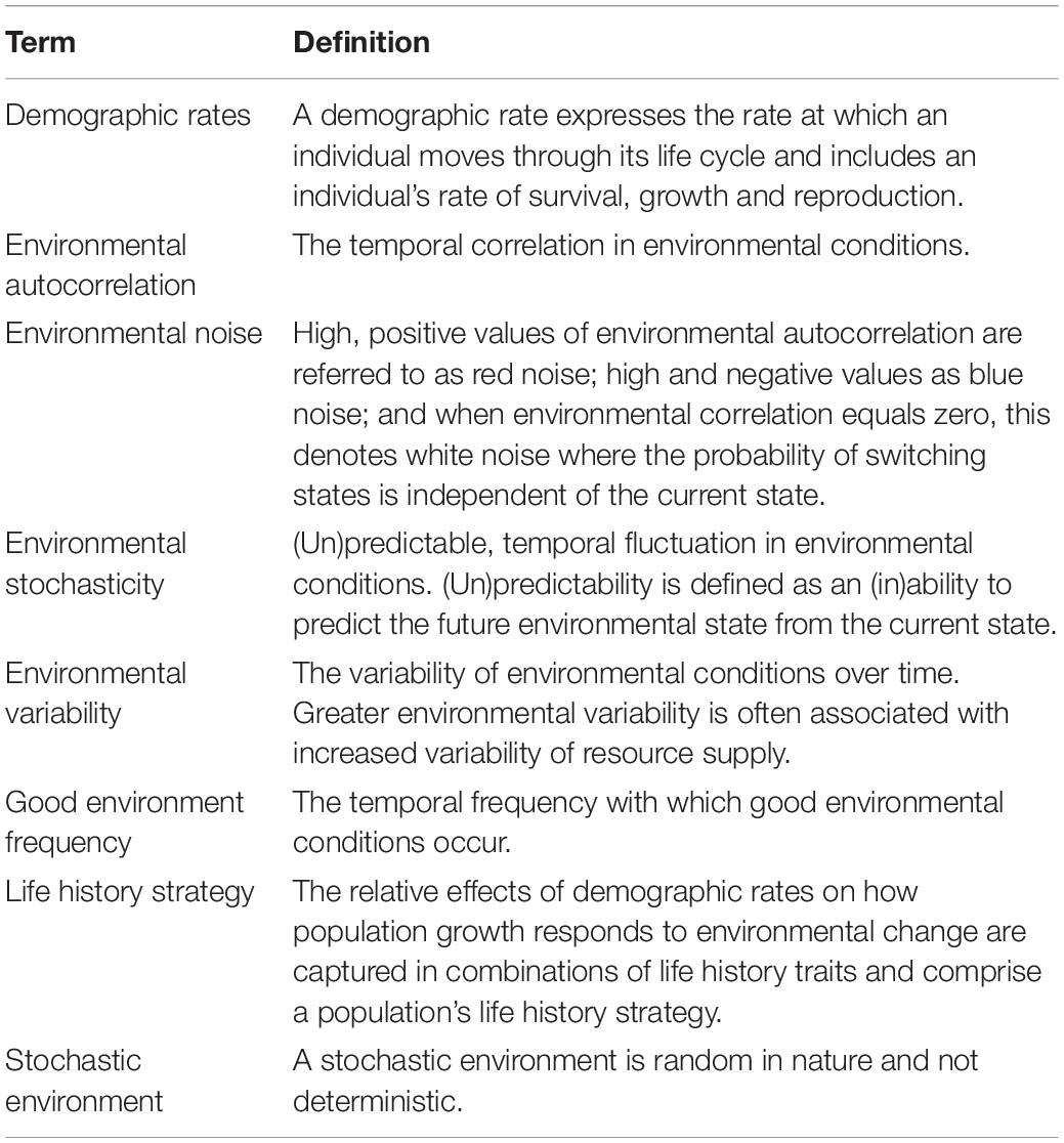
Table 1. Definitions of important terms.

Marine megafauna are globally recognized as providing significant economic, cultural, and ecological values (Bakker et al., 2016; Teh et al., 2018). Despite this, many marine megafauna species have experienced population declines, putting some species at risk of extinction (Paleczny et al., 2010; Davidson et al., 2012; Randhawa et al., 2015). Charismatic marine megafauna that inhabit coastalscapes are mobulid rays, carcharhinid sharks and cheloniid sea turtles. They fulfill key roles as predators or grazers in coastal ecosystems in the (sub)tropics (Ferretti et al., 2010; Roff et al., 2016), yet their persistence is threatened by (over)fishing, loss of breeding habitat, pollution, habitat disturbance and pathogens (Clarke et al., 2006; Estes et al., 2011; Brooks et al., 2013; Mourier and Planes, 2013; Vianna et al., 2013; Ward-Paige et al., 2013; Dwyer et al., 2020; Jatmiko and Catur Nugroho, 2020). As a result, most of these marine megafauna are now listed as vulnerable, near-threatened or endangered on the international union for conservation of nature red list of threatened species (Marshall et al., 2011; Brooks et al., 2013).

Mobulids, carcharhinids and cheloniids all have several slow life history characteristics in common (Heppell et al., 1999; Musick, 1999): they are all long-lived [20–30 years for many carcharhinids (Ward-Paige et al., 2010); > 40 years for many mobulids (Marshall et al., 2011) and > 60 years for cheloniids (Chaloupka and Limpus, 2005)], mature relatively late in life [5–10 years for carcharhinids and mobulids (Branstetter, 1987; Kneebone et al., 2008; Marshall et al., 2011); 20–40 years for cheloniids (Davenport, 1997; Zug et al., 1997; Casale et al., 2003; Broderick et al., 2003)], and display relatively slow, physiological growth and development (Killam and Parsons, 1989; Davenport, 1997; Zug et al., 1997; Casale et al., 2003; Broderick et al., 2003). Reproductive strategies, however, differ markedly between cheloniids, and the mobulids and carcharhinids. Whereas mobulids and carcharhinids are live-bearing, producing on average 1–5 pups per breeding event (Wetherbee et al., 1997; Ward-Paige et al., 2010; Marshall et al., 2011; Whitney et al., 2012), characteristic of slow life histories [Stearns, 1992; but note that, e.g., the tiger shark Galeocerdo cuvier can produce up to 80 pups per breeding event (Hammerschlag et al., 2018)], cheloniids can lay hundreds of eggs within one nesting season (Heppell et al., 1996a, b; Miller, 1997; Broderick et al., 2003), characteristic of fast life histories (Stearns, 1992). These large differences in reproductive strategy lead to large differences in juvenile mortality rates, which are relatively low for mobulids and carcharhinids, characteristic of slow life histories [Stearns, 1992; but note again that juvenile mortality is high in the tiger shark (Ward-Paige et al., 2010)], and very high for cheloniids (Heppell et al., 1996a, b; Miller, 1997; Broderick et al., 2003), characteristic of fast life histories (Stearns, 1992). With ongoing climate change impacting ecosystems worldwide, an urgent question is how the subtly different life history strategies of mobulids, carcharhinids and cheloniids buffer or intensify their demographic responses to climate change induced shifts in environmental stochasticity (Table 1; Carr et al., 1978; Morreale et al., 1982; Limpus and Reed, 1985; Janzen, 1994; Hawkes et al., 2009; Mourier et al., 2013; Moffitt et al., 2015; Marn et al., 2017a). This requires in depth understanding of their demographic responses to shifts in environmental autocorrelation and good environment frequency (Table 1), and the physiological processes that drive these (Marn et al., 2017b), which is all essential for the successful conservation management of marine megafauna (Cortés, 2002; Oh et al., 2017; Byrne et al., 2019).

Here we use a life history trait approach to explore if the subtly different life history strategies of mobulid rays, carcharhinid sharks and cheloniid sea turtles are differentially sensitive to environmental autocorrelation and good environment frequency. We describe individual life histories from a dynamic energy budget (DEB) perspective, and examine how the environment affects the change in individual life histories, thereby generating the dynamics of population structure (Webb et al., 2010). Such an approach can offer mechanistic insights into how individual level processes affect population responses to environmental change. The traditional approach to do so is to use physiologically structured population models (PSPMs). However, the analysis of PSPMs requires rather complicated methodology and PSPMs typically are more mathematical representations of biological systems (deRoos and Persson, 2013). We therefore resort to using the recently developed DEB integral projection model (DEB-IPM; Smallegange et al., 2017). In contrast to PSPMs, IPMs are data-driven, provide a way of synthesizing complex life history information and can be analyzed using more straightforward mathematical techniques (Smallegange and Coulson, 2013). The DEB-IPM takes data on individual life histories as input parameters to describe growth and reproduction following a simple version of the standard model of Kooijman’s DEB theory (Kooijman, 2010), also known as the Kooijman-Metz model (Kooijman and Metz, 1984). Mortality and the association between parent and offspring characteristics do not follow DEB theory, and are estimated from individual-level observations (Smallegange et al., 2017).

Using the DEB-IPM, we examine population-level responses in fitness and in mean size (as a proxy for population structure) to a wide range of environmental autocorrelation and good environment frequency values, and ask (i) if the overall slower mobulid and carcharhinid life histories show higher sensitivities of log stochastic population growth rates, log(λ_s), to environmental autocorrelation than the turtles that also display some fast life history characteristics, (ii) if the different life histories show different sensitivities of log(λ_s) to good environment frequency, and (iii) if the log(λ_s) responses can be captured by any of the life history traits within the DEB-IPM (mortality, growth, reproduction) along an axis of life history speed. We parameterized DEB-IPMs for four species of mobulid rays, five species of carcharhinid sharks, and four species of cheloniid sea turtle. For each species, we carried out stochastic simulations to assess if they show high or low sensitivity of log(λ_s) and of mean body size to shifts in environmental autocorrelation and good environment frequency. Environments with varying environmental autocorrelation and good environment frequency were simulated using a stochastic demographic model in which the temporal sequence of good and bad food environments is driven by a Markovian process that governs the serial correlation of environment states. In order to cover a wide range of such stochastic environments (Table 1), we varied this serial correlation from blue to white to red environmental noise color (corresponding to a negative first-order autocorrelation, no autocorrelation, and a positive first-order autocorrelation of the temporal sequence, respectively; Table 1) for two values of good environment frequency. Next, we varied good environment frequency from almost zero to almost one, in the absence of environmental autocorrelation (white noise: Table 1). Finally, across stochastic environments, we conducted perturbation analyses to assess which functional trait had the strongest effect on log(λ_s), and we assessed how functional traits relate to variation in log(λ_s). Our approach allows us to assess whether the effects of environmental autocorrelation and good environment frequency on a select group of marine megafauna demography can be predicted from the life history traits that comprise each species’ life history strategy.

Methods

Brief Description of the DEB-IPM

The demographic functions that describe growth and reproduction in the DEB-IPM are derived from the Kooijman-Metz model (Kooijman and Metz, 1984), which is a simple version of the standard model of Kooijman’s DEB theory, but still fulfils the criteria for general explanatory models for the energetics of individuals (Sousa et al., 2010). The Kooijman-Metz model assumes that individual organisms are isomorphic (body surface area and volume are proportional to squared and cubed length, respectively). The rate at which an individual ingests food, I, is assumed to be proportional to the maximum ingestion rate I_max, the current feeding level Y and body surface area, and hence to the squared length of an organism: I = I_maxYL². Ingested food is assimilated with a constant efficiency ε. A constant fraction κ of assimilated energy is allocated to soma (metabolic maintenance and growth); this energy equals κεI_maxYL² and is used to first cover maintenance costs, which are proportional to body volume following ξL³ (ξ is the proportionality constant relating maintenance energy requirements to cubed length), while the remainder is allocated to somatic growth. The remaining fraction 1–κ of assimilated energy, the reproduction energy, is allocated to reproduction in case of adults and to the development of reproductive organs in case of juveniles, and equals (1−κ)εI_maxYL². This means that, if an individual survives from year t to year t + 1, it grows from length L to length L′ following a von Bertalanffy growth curve, $\frac{dL}{dt}={\stackrel{.}{r}}_{\text{B}}\left(L_m\cdot \text{Y–L}\right)$, where r_B is the von Bertalanffy growth rate and L_m = κεI_max/ξ is the maximum length under conditions of unlimited resource. Both κ and I_max are assumed to be constant across experienced feeding levels, and therefore L_m is also assumed constant. If a surviving female is an adult, she also produces offspring. According to the Kooijman-Metz model, reproduction, i.e., the number of offspring produced by an individual of length L between time t and t + 1, equals $Y\cdot R_{\text{m}}\cdot L^2/L_{\text{m}}^2$. The parameter R_m is the maximum reproduction rate of an individual of maximum length L_m. Note that R_m is proportional to (1–κ) (Kooijman and Metz, 1984), whereas L_m is proportional to κ, which controls energy conservation. However, the role of κ in the DEB-IPM is mostly implicit, as κ is used as input parameter only in the starvation condition (see below), whereas R_m and L_m are measured directly from data. Like L_m, R_m is also proportional to I_max; since both κ and I_max are assumed to be constant across experienced feeding levels, R_m is also assumed constant.

The above individual life history events are captured in the DEB-IPM by four fundamental functions to describe the dynamics of a population comprising cohorts of females of different sizes (Smallegange et al., 2017): (1) the survival function, S(L(t)) (unit: y^–1), describing the probability of surviving from year t to year t + 1; (2) the growth function, G(L′,L(t)) (unit: y^–1), describing the probability that an individual of body length L at year t grows to length L′ at t + 1, conditional on survival; (3) the reproduction function, R(L(t)) (unit: # y^–1), giving the number of offspring produced between year t and t + 1 by an individual of length L at year t; and (4) the parent-offspring function, D(L′,L(t)) (unit: y^–1), the latter which describes the association between the body length of the parent L and offspring length L′ (i.e., to what extent does offspring size depend on parental size). The DEB-IPM assumes no effect of temperature on fundamental functions. Denoting the number of females at year t by N(L,t) means that the dynamics of the body length number distribution from year t to t + 1 can be written as:

$N(L^{\prime },t+1)={\int }_{\mathrm{\Omega }}\left[D(L^{\prime },L(t))R\left(L\left(t\right)\right)+G(L^{\prime },L(t))S(L(t))\right]N(L,t)\mathit{d}L(1)$

where the closed interval Ω denotes the length domain. Implicitly underlying the population-level model of eqn 1, like in any IPM, is a stochastic, individual-based model, in which individuals follow Markovian growth trajectories that depend on an individual’s current state (Easterling et al., 2000). This individual variability is in standard IPMs modeled in the functions describing growth, G(L′,L(t)), and the parent-offspring association,D(L′,L(t)), using a probability density distribution, typically Gaussian (Easterling et al., 2000). In the DEB-IPM, this individual variability arises from how individuals experience the environment; specifically, the experienced feeding level Y follows a Gaussian distribution with mean E(Y) and standard deviation σ(Y). It means that individuals within a cohort of length L do not necessarily experience the same feeding level due to demographic stochasticity (e.g., individuals, independently of each other, have good or bad luck in their feeding experience).

The survival function S(L(t)) in Eq. 1 is the probability that an individual of length L survives from year t to t + 1:

$S(L(t))=\{\begin{array}{cc}{e}^{-{\mathrm{\mu }}_{\text{j}}}\mathit{\hspace{1em}}\hfill & \text{for}{L}_b\le L<L_p\&L\le L_{m}E(Y)/\mathrm{\kappa },\hfill \\ e^{-{\mathrm{\mu }}_{\text{a}}}\mathit{\hspace{1em}}\hfill & \text{for}{L}_p\le L\le L_m\&L\le L_{m}E(Y)/\mathrm{\kappa },\hfill \\ 0\mathit{\hspace{1em}}\hfill & otherwise\hfill \end{array}(2)$

where E(Y) can range from zero (empty gut) to one (full gut). Here, individuals that experience E(Y) = 1 can be assumed to always have a full gut. Individuals die from starvation at a body length at which maintenance requirements exceed the total amount of assimilated energy, which occurs when L > L_m⋅E(Y)/κ and hence, then, S(L(t)) = 0 (e.g., an individual of size L_m will die of starvation if E(Y) < κ). Juveniles and adults often have different mortality rates, and, thus, juveniles (L_b≤L < L_p) that do not die of starvation (i.e., L≤L_m⋅E(Y)/κ) have a mortality rate of μ_j, and adults (L_p≤L≤L_m) that do not die of starvation (i.e., L≤L_m⋅E(Y)/κ) have a mortality rate of μ_a.

The function G(L′,L(t)) is the probability that an individual of body length L at year t grows to length L′ at t + 1, conditional on survival, and, following common practice (Easterling et al., 2000; Coulson, 2012; Merow et al., 2014), follows a Gaussian distribution:

$G(L^{\prime },L(t))=\frac{1}{\sqrt{2\mathrm{\pi }{\mathrm{\sigma }}_{\text{L}}^2\left(L(t+1)\right)}}{e}^{\frac{-(L^{\prime }-E{\left(L(t+1)\right)}^2}{2{\mathrm{\sigma }}_{\text{L}}^2\left(L(t+1)\right)}}(3)$

with the growth realized by a cohort of individuals with length L(t) equaling

$E\left(L\left(t+1\right)\right)=\{\begin{array}{cc}L\left(t\right)e^{-{\stackrel{\_}{r}}_{\text{B}}}+(1-e^{-{\stackrel{\_}{r}}_{\text{B}}})L_{\text{m}}E\left(Y\right)forL\le L_{m}E(Y),\hfill & \\ L\left(t\right)\mathit{\hspace{1em}\hspace{1em}\hspace{1em}\hspace{1em}\hspace{1em}\hspace{1em}\hspace{1em}\hspace{1em}\hspace{1em}\hspace{1em}\hspace{0.5em}\hspace{0.25em}}otherwise\mathit{\hspace{1em}}\hfill & \end{array}(4)$

assuming individuals do not shrink under starvation conditions (Smallegange et al., 2017), and the variance in length at time t + 1 for a cohort of individuals of length L as

${\mathrm{\sigma }}^2\left(L(t+1)\right)=\{\begin{array}{cc}{(1-e^{-{\stackrel{\_}{r}}_{\text{B}}})}^2{L}_{\text{m}}^2{\mathrm{\sigma }}^2\left(Y\right)forL\le L_{m}E(Y),\hfill & \\ 0\mathit{\hspace{1em}}\mathit{\hspace{1em}\hspace{1em}\hspace{1em}\hspace{1em}\hspace{1em}\hspace{1em}\hspace{1em}\hspace{0.5em}\hspace{0.25em}}otherwise\hfill \end{array}(5)$

where σ(Y) is the standard deviation of the expected feeding level.

The reproduction function R(L(t)) gives the number of offspring produced between year t and t + 1 by an individual of length L at year t:

$R\left(L(t)\right)=\{\begin{array}{c}\hfill 0\mathit{\hspace{1em}\hspace{1em}\hspace{1em}\hspace{1em}\hspace{1em}\hspace{1em}\hspace{1em}\hspace{1em}\hspace{1em}\hspace{1em}\hspace{1em}\hspace{1em}\hspace{1em}\hspace{1em}\hspace{1em}\hspace{1em}\hspace{1em}\hspace{1em} }\mathrm{for}{L}_b\le L<L_p\hfill \\ \hfill E\left(Y\right)R_{m}L{\left(t\right)}^2/L_m^2\mathrm{for}{L}_p\le L\le L_{m}E(Y)\hfill \\ \hfill \frac{R_m}{1-\mathrm{\kappa }}\left[E\left(Y\right)L{\left(t\right)}^2-\frac{\mathrm{\kappa }L{(t)}^3}{L_m}\right]\mathrm{for}{L}_{m}E(Y)<L\le L_{m}E(Y)/\mathrm{\kappa }\hfill \end{array}(6)$

Individuals are mature when they reach puberty at body length L_p and only surviving adults reproduce (Eq. 1); thus, only individuals within a cohort of length L_p≤L≤L_mY/κ reproduce. When maintenance costs cannot be covered (starvation), ingested energy is rechannelled from reproduction to maintenance, which occurs for L > L_mE(Y).

The probability density function D(L′,L(t)) gives the probability that the offspring of an individual of body length L are of length L′ at year t + 1, and hence describes the association between parent and offspring character values:

$D(L^{\prime },L\left(t\right))=\{\begin{array}{cc}0\mathit{\hspace{1em}}\hfill & \text{for}L<L_p\hfill \\ \frac{1}{\sqrt{2\mathrm{\pi }{\mathrm{\sigma }}_{L_{\text{b}}}^2\left(L\left(t\right)\right)}}{e}^{\frac{-(L^{\prime }-E_{L_{\text{b}}}{\left(L\left(t\right)\right)}^2}{2{\mathrm{\sigma }}_{L_{\text{b}}}^2\left(L\left(t\right)\right)}}\mathit{\hspace{1em}}\hfill & \text{otherwise}\hfill \end{array}(7)$

where E_Lb (L(t)) is the expected size of offspring produced by a cohort of individuals with length L(t), and ${\mathrm{\sigma }}_{L_{\text{b}}}^2(L\left(t\right))$ the associated variance. For simplicity, we set E_Lb (L(t)) constant and assumed its associated variance,${\mathrm{\sigma }}_{L_{\text{b}}}^2\left(L\left(t\right)\right)$, to be very small.

Parameterization of the DEB-IPM

We took values for the fraction of assimilated energy allocated to maintenance and growth, κ, from the Add My Pet database (Add-my-pet, 2020), if available, and otherwise assumed κ = 0.8, as in the generalized animal (Kooijman, 2010; Table 2); mortality rates are all estimates of natural mortality rates. Most parameter estimates were taken directly from the literature (references in Table 2), but for some species they had to be calculated from other life history parameters, which is explained below.

TABLE 2

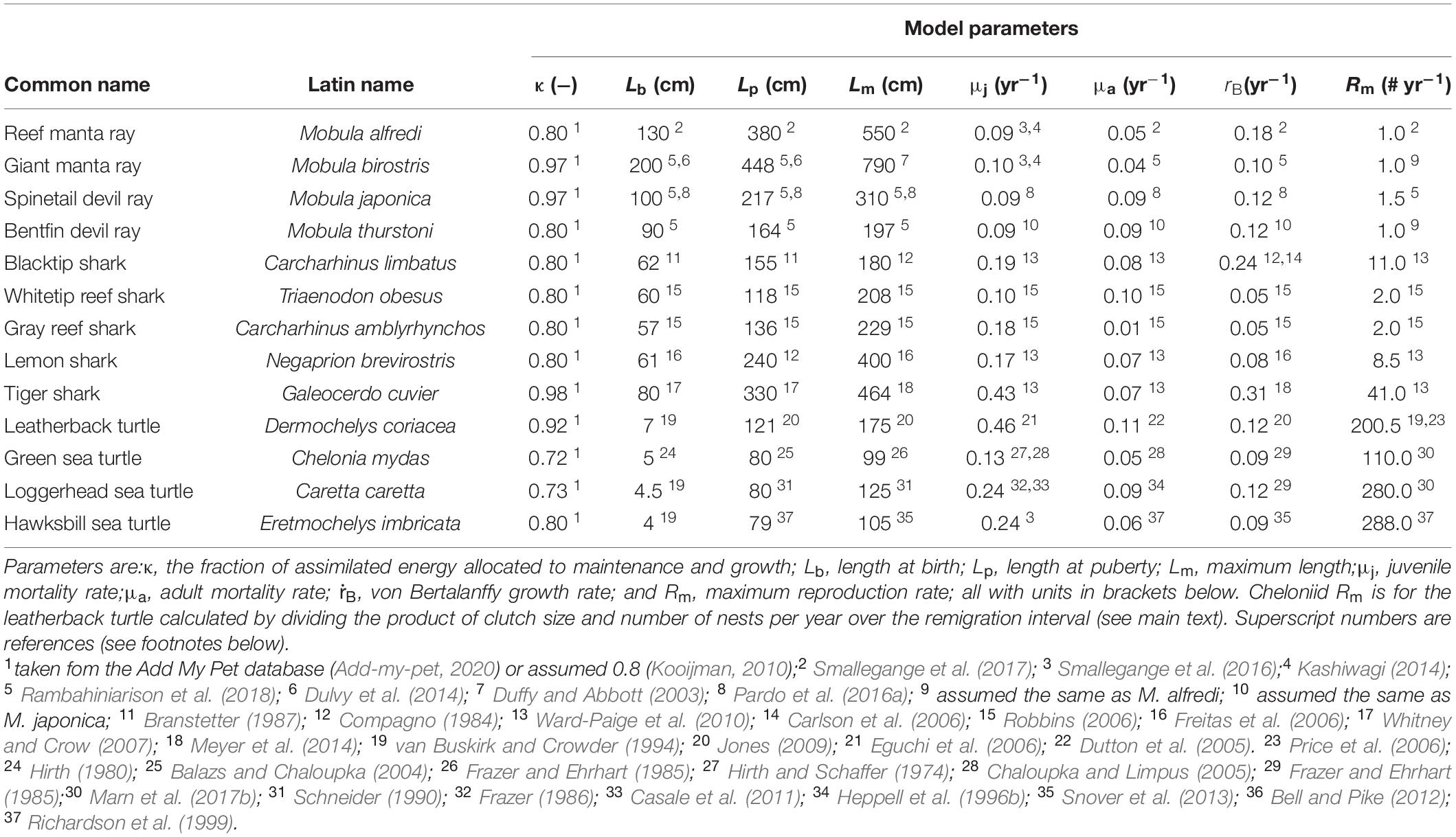
Table 2. Model parameters for the mobulid, carcharhinid and cheloniid species.

Mobulid Rays

In case of M. alfredi, we calculated juvenile mortality rate μ_i from its yearling survival rate (P_y = 0.63 yr^–1), its juvenile survival rate (P_j = 0.95 yr^–1) and its average age at maturity (α = 10; Kashiwagi, 2014; Smallegange et al., 2016): ${\mathrm{\mu }}_{\text{i}}=-\text{log}\left(\sqrt[10]{P_{\text{y}}\times P_{\text{j}}^9}\right)$ (Table 2), assuming P = e^−μ (Caswell, 2001). In case of M. birostris, we were unable to find estimates for μ_i. We instead took M. alfredi yearling survival rate (P_y = 0.63 yr^–1) and juvenile survival rate (P_j = 0.95 yr^–1; Kashiwagi, 2014; Smallegange et al., 2016), and, given the fact that M. birostris matures on average at 9 years of age (Dulvy et al., 2014; Rambahiniarison et al., 2018), ${\mathrm{\mu }}_{\text{i}}=-\text{log}\left(\sqrt[9]{P_{\text{y}}\times P_{\text{j}}^8}\right)$ (Table 2). We also could not find an estimate for M. birostris R_m and therefore assumed it equaled that of M. alfredi (Table 2). Finally, in case of M. thurstoni, we were unable to find estimates for μ_j and μ_a, and assumed these to equal those of M. japanica (Table 2).

Carcharhinids Sharks

In case of C. limbatus, N. brevirostris, and G. cuvier we calculated juvenile mortality rate, μ_j, as μ_j = −log $\left(\sqrt[\text{α}]{P_{\text{m}}}\right)$ with P_m as the survival probability from newborn to maturity, and α as average age at maturity (yr). In case of C. limbatus, P_m = 0.26 and α = 7 yr; in case of N. brevirostris, P_m = 0.12 and α = 12.7 yr, and in case of G. cuvier, P_m = 0.02 and α = 9 yr (Ward-Paige et al., 2010; Table 2). For the latter three species, adult mortality rate, μ_a, was calculated as μ_a = −log $\left(\sqrt[l]{P_{\text{a}}}\right)$, where P_a is the natural mortality rate over the adult life span, l. For C. limbatus, P_a = 0.25 and l = 18 yr; for N. brevirostris, P_a = 0.18 and l = 25 yr, and for G. cuvier, P_a = 0.68 and l = 28 yr (Table 2). In case of T. obesus and C. amblyrhynchos, μ_j and μ_a were calculated from life tables of age-specific, yearly survival rates (Robbins, 2006).μ_j = −log $\left(\sqrt[\text{α}-1]{P_1\times P_2\times \dots \times P_{\text{α}-1}}\right)$ and μ_a = −log $\left(\sqrt[1]{P_{\text{α}}\times P_{\text{α}+1}\times \dots \times P_1}\right)$ (Table 2).

Cheloniid Turtles

In case of C. mydas, C. caretta and E. imbricata we calculated μ_i as μ_j = −log $\left(\sqrt[\text{α}]{P_{\text{m}}}\right)$. In case of C. mydas, P_m = 0.01 [as 10 out of 1,000 eggs need to survive for a population to persist (Hirth and Schaffer, 1974)] and α = 35 yr (Chaloupka and Limpus, 2005); in case of C. caretta, P_m = 0.025 [as 2.5 out of 1,000 eggs need to survive for a population to persist (Frazer, 1986)] and α = 26 yr (Casale et al., 2011); and in case of E. imbricata, P_m = 0.01 (we assumed, like C. mydas, that 10 out of 1,000 eggs need to survive for a population to persist) and α = 30 yr (Limpus, 1992; Chaloupka and Limpus, 1997; Table 2). For all cheloniid species, adult mortality rate, μ_a, was calculated as μ_a = −log(P_s), where P_s is the annual adult survival rate. For D. coriacea, P_s = 0.89 (Dutton et al., 2005); for C. mydas, P_s = 0.95 (Chaloupka and Limpus, 2005); for C. caretta, P_s = 0.91 (Heppell et al., 1996b); and for E. imbricata, P_s = 0.94 (Richardson et al., 1999; Table 2). Finally, in case of D. coriacea, we calculated maximum reproduction rate R_m as R_m = (c×n)/i, where c is the mean clutch size of a single nest, n is the mean number of nests produced per year, and i is the remigration interval, which is the minimal number of years between reproductive seasons (Table 2). For all other sea turtles, R_m was taken directly from the literature (Table 2).

Stochastic Demographic Model

We used the stochastic demographic model p(t + 1) = A(t)⋅p(t), where p(t) is the population vector at time t and A(t) is a DEB-IPM at time t defined by a two-state Markov chain that gives the probability distribution of environment states at time t. In this chain, state 1 is the good environment and state 2 is the bad environment. This results in the following Markov chain habitat transition matrix H (Caswell, 2001, p. 379):

$\mathbf{\text{H}}=\left[\begin{array}{cc}\hfill 1-p\mathit{\hspace{1em}}\hfill & \hfill q\hfill \\ \hfill p\mathit{\hspace{1em}}\hfill & \hfill 1-q\hfill \end{array}\right](8)$

where p is the probability of switching from the good to the bad environment, and q is the probability of switching from the bad to the good environment. The serial or autocorrelation of the Markov chain equals ρ = 1–p–q (Caswell, 2001, p. 379). High, positive values of ρ are referred to as red noise; high and negative values of ρ as blue noise; and ρ = 0 denotes white noise where the probability of switching states is independent of the current state (Table 1). The good environment frequency is given by f = q/(p + q) (Caswell, 2001, p. 379). We used a high feeding level E(Y)_high and a low feeding level E(Y)_low to define the good and bad environmental states, respectively. Specifically, E(Y)_low is the expected feeding level associated with population decline (λ < 1) and E(Y)_high as the expected feeding level associated with population increase (λ > 1). For the rays and sharks, we set E(Y)_low = 0.7 and E(Y)_high = 1.0 and for the turtles that have a slightly faster life history speed, we set E(Y)_low = 0.6 and E(Y)_high = 1.0 (Smallegange and Berg, 2019). We set σ(Y) = 0.3. We aimed to independently study the effects of environmental autocorrelation ρ and good environment frequency f (Table 1). We thus varied ρ across the full noise gradient, while keeping f fixed at f = 0.5; and over a gradient of white and red noise, while keeping f fixed at f = 0.75. We varied f across the full gradient ranging from almost zero to almost unity, while keeping ρ constant at ρ = 0.5. Each stochastic simulation was generated in MatLab (MATLAB. version 9.2.0.556344 [R2017a], The MathWorks, Inc., Natick, MA, United States) by iterating H over a time series of length 50,000 (with an initial transient length of 500 discarded, a starting population of one individual in each size bin, and with the initial environment state chosen randomly [see also Tuljapurkar et al., 2003]; e.g., Smallegange et al., 2014). This sequence determines the environment state, and hence the feeding level E(Y), that a population experiences at each time step, from which the individual-level functions were calculated to construct A(t), i.e., the DEB-IPM at time t defined by the feeding level E(Y) at time t. At each time step, A(t) was stored with associated vectors of population structure to calculate the log of the stochastic population growth rate λ_s as $\text{log}({\mathrm{\lambda }}_s)=\frac{1}{\mathrm{\tau }}{\sum }_{\mathrm{\tau }=0}^{\mathrm{\tau }-1}{r}_{\text{t}}$ with r_t = log[p(t + 1)/p(t)], where τ = 50,000 – 500 = 49,500. At each time step, also the mean of the body size distribution was calculated, after which we used the pooled mean body size, calculated as the grand mean of all mean body sizes over time period τ, for our analysis. For a given species, a decrease in pooled mean body size across a stochastic gradient would indicate an increase in the proportion of juveniles in the population, where an increase in pooled mean body size would indicate an increase in the proportion of adults in the population.

Perturbation Analysis

We conducted a perturbation analysis in MatLab (MATLAB. version 9.2.0.556344 [R2017a]) to examine the elasticity of the log stochastic population growth rate, log(λ_s), to perturbation of each of the life history parameters: length at birth L_b, length at puberty L_p, maximum length L_m, juvenile mortality rate μ_j, adult mortality rate μ_a, von Bertalanffy growth rate ${\stackrel{.}{r}}_{\text{B}}$, and maximum reproduction rate R_m (Table 2). This analysis allows us to identify which life history parameter is most influential to log(λ_s), and if this depends on the type of stochastic environment. In order to do this, we perturbed each parameter by 1% and calculated the elasticity of log(λ_s) to each model parameter. We excluded the parameter κ(fraction of assimilated energy allocated to maintenance and growth), because it cannot be perturbed directly as, apart from occurring in the starvation condition (Eq. 2), it is implicitly included in the model within L_m (which is mathematically proportional to κ) and R_m (which is mathematically proportional to [1–κ]; Kooijman and Metz, 1984).

Linking Life History Parameters to log(λ_s) Across Stochastic Environments

Four of the model parameters are life history characteristics that place species on the fast-slow life history continuum. Specifically, fast (or slow) life histories are characterized by high (or low) mortality rate μ_j and μ_a, high (or low) individual growth rate ${\stackrel{.}{r}}_{\text{B}}$, high (or low) reproduction rate R_m (Gaillard et al., 1989: Stearns, 1992; Salguero-Gómez et al., 2016). It would thus be interesting to assess if the magnitude change in log(λ_s) over the environmental autocorrelation, ρ, or good environment frequency, f, gradient is linked to species-specific parameter values. For example, the reef manta ray M. alfredi, a slow life history species, characterized by low values of μ_j, μ_a, ${\stackrel{.}{r}}_{\text{B}}$, and R_m, is more sensitive to a change in environmental autocorrelation than the fast life history species O. gammarellus, characterized by high values of μ_j, μ_a, ${\stackrel{.}{r}}_{\text{B}}$, and R_m (Smallegange and Berg, 2019). In a cross-species comparison, you would then expect a correlation between the values of μ_j, μ_a, ${\stackrel{.}{r}}_{\text{B}}$, and R_m and the magnitude with which the log stochastic population growth rate, log(λ_s), responds to changes in ρ. To this end, we first normalized (scaled) ${\stackrel{.}{r}}_{\text{B}}$ and R_m to compare across species (μ_j, μ_a already only take values between zero and unity), and then used a linear model with each (normalized) model parameter as a continuous explanatory variable to test its relationship to the difference between log(λ_s) at the end and at the start of each stochastic gradient. Analyses were carried out in MatLab (MATLAB. version 9.2.0.556344 [R2017a]).

Results

Shifts in log(λ_s) and Pooled Mean Body Size Across Stochastic Environments

Across the gradient of environmental autocorrelation ρ, the log stochastic population growth rate, log(λ_s), of mobulids increased as ρ increased from zero (white noise) to high positive (red noise), both when good environment frequency f is fixed at f = 0.5 and f = 0.75 (Figure 1A). For all mobulid species, log(λ_s) was higher when f is fixed at f = 0.75 (gray lines in Figure 1A) then when f = 0.5 (black lines in Figure 1A). Carcharhinids log(λ_s) values were hardly affected by environmental autocorrelation, except for the tiger shark (G. cuvier), for which log(λ_s) showed a hump-shaped response over the environmental autocorrelation gradient (Figure 1B). Like the mobulids, log(λ_s) of the carcharhinids was higher when f is fixed at f = 0.75 (gray lines in Figure 1B) than when f = 0.5 (black lines in Figure 1B), particularly for the tiger shark G. cuvier. Cheloniid log(λ_s) was the least sensitive to temporal autocorrelation, because log(λ_s) for most species only decreased very slightly over the environmental autocorrelation ρ gradient before showing a small but sudden drop in value as ρ approached unity (Figure 1C). Like the mobulids and most carcharhinids, cheloniid log(λ_s) was higher when good environment frequency f is fixed at f = 0.75 (gray lines in Figure 1C) than when f = 0.5 (black lines in Figure 1C). Across the gradient of good environment frequency f (while keeping ρ = 0), log(λ_s) increased for all species, but the increase was greater for carcharhinids and cheloniids, than for mobulids (Figures 1D,E).

FIGURE 1

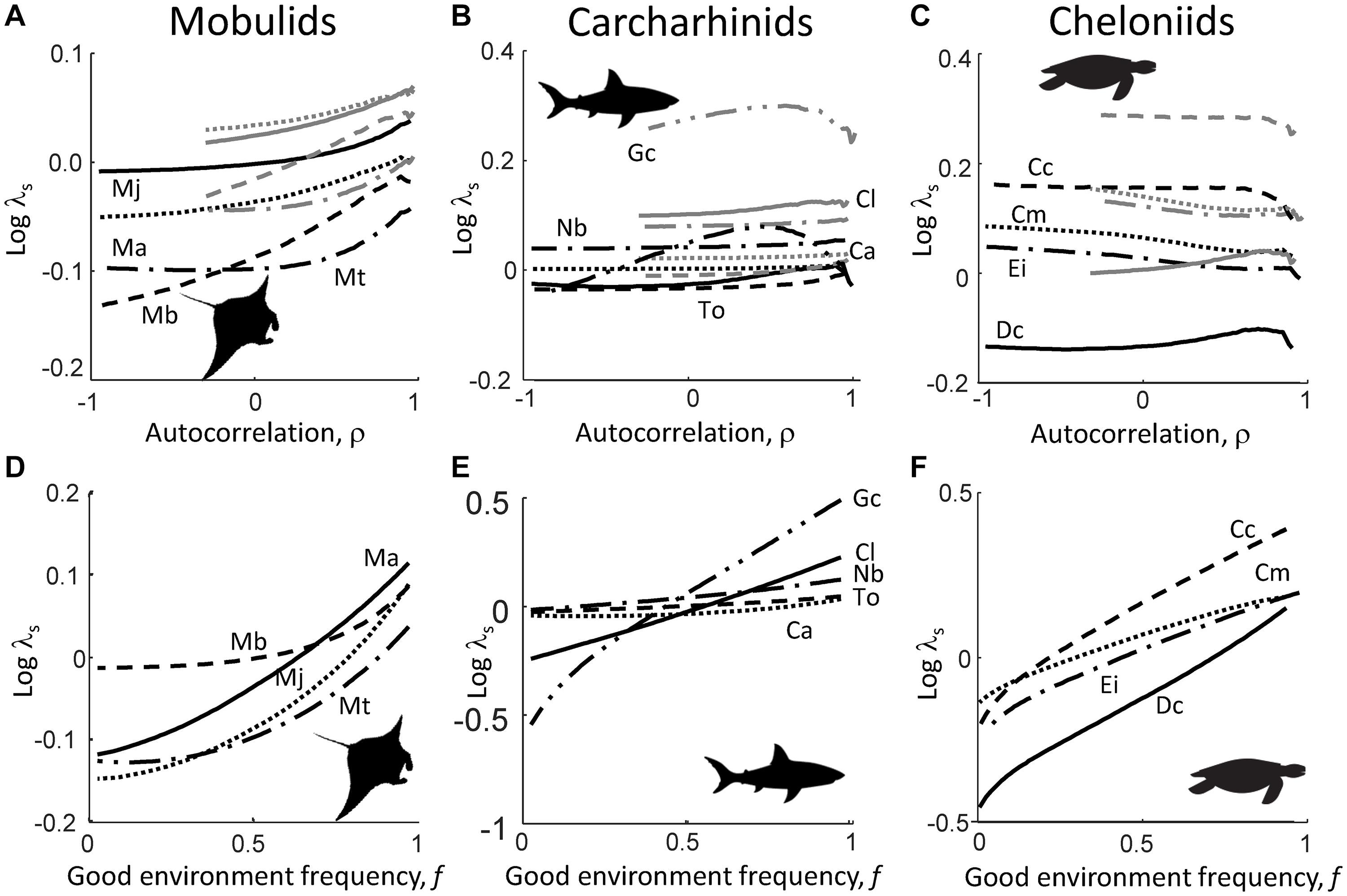
Figure 1. Shifts in the log stochastic population growth rate, log(λ_s), across the gradient of environmental autocorrelation ρ ranging from negative (blue noise), zero (white noise) and positive (red noise) for mobulids (A), carcharhinids (B), and cheloniids (C); and shifts in log(λ_s) across the gradient of good environment frequency f ranging from almost zero (stochastic environments are characterized by predominantly bad food conditions) to almost unity (stochastic environments are characterized by predominantly good food conditions) for mobulids (D), carcharhinids (E), and cheloniids (F). Black lines in the top panels are log(λ_s) values when the good environment frequency is fixed at f = 0.5; gray lines in the top panels when f = 0.75. Mobulid species are M. alfredi (Ma; solid lines), M. birostris (Mb; dotted lines), M. japonica (Mj; dashed lines), and M. thurstoni (Mj; dash-dot lines); carcharhinid species are C. limbatus (Cl; solid lines), T. obesus (To; dotted lines), C. amblyrhynchos (Ca; dashed lines), N. brevirostris (Nb; dash-dot lines), and G. cuvier (Gc; dash-dot-dot lines); cheloniid species are D. coriacea (Dc; solid lines), C. mydas (Cm; dotted lines), C. caretta (Cc; dashed lines), and E. imbricatea (Ei; dash-dot lines). Note difference in y-scale between (A) versus (B) and (C), and (D) versus (E) and (F).

Pooled mean body size of mobulids and carcharhinids (Figures 2A,B) was largely insensitive to shifts in environmental autocorrelation ρ, both when good environment frequency f is fixed at f = 0.5 and f = 0.75 (Figures 2A,B), and was also largely insensitive to shifts in good environment frequency f (Figures 2D,E). The exception to the latter patterns was the tiger shark (G. cuvier), for which pooled mean body size increased with increasing ρ, both when f is fixed at f = 0.5 and f = 0.75 (Figure 2B), and decreased with increasing f (Figure 2E). In contrast, pooled mean body size of cheloniids increased with increasing values of environmental autocorrelation ρ, with a sudden, sharp increase as ρ approached unity, both when f is fixed at f = 0.5 and f = 0.75 (Figure 2C), whereas it decreased with increasing values of f (Figure 2F). Finally, overall, pooled mean body size across the environmental autocorrelation ρ gradient was for some species, like the tiger shark (G. cuvier) and leatherback turtle (D. coriacea) higher when f = 0.75, than when f = 0.5, although the extent of this difference varied between species (Figures 2A–C).

FIGURE 2

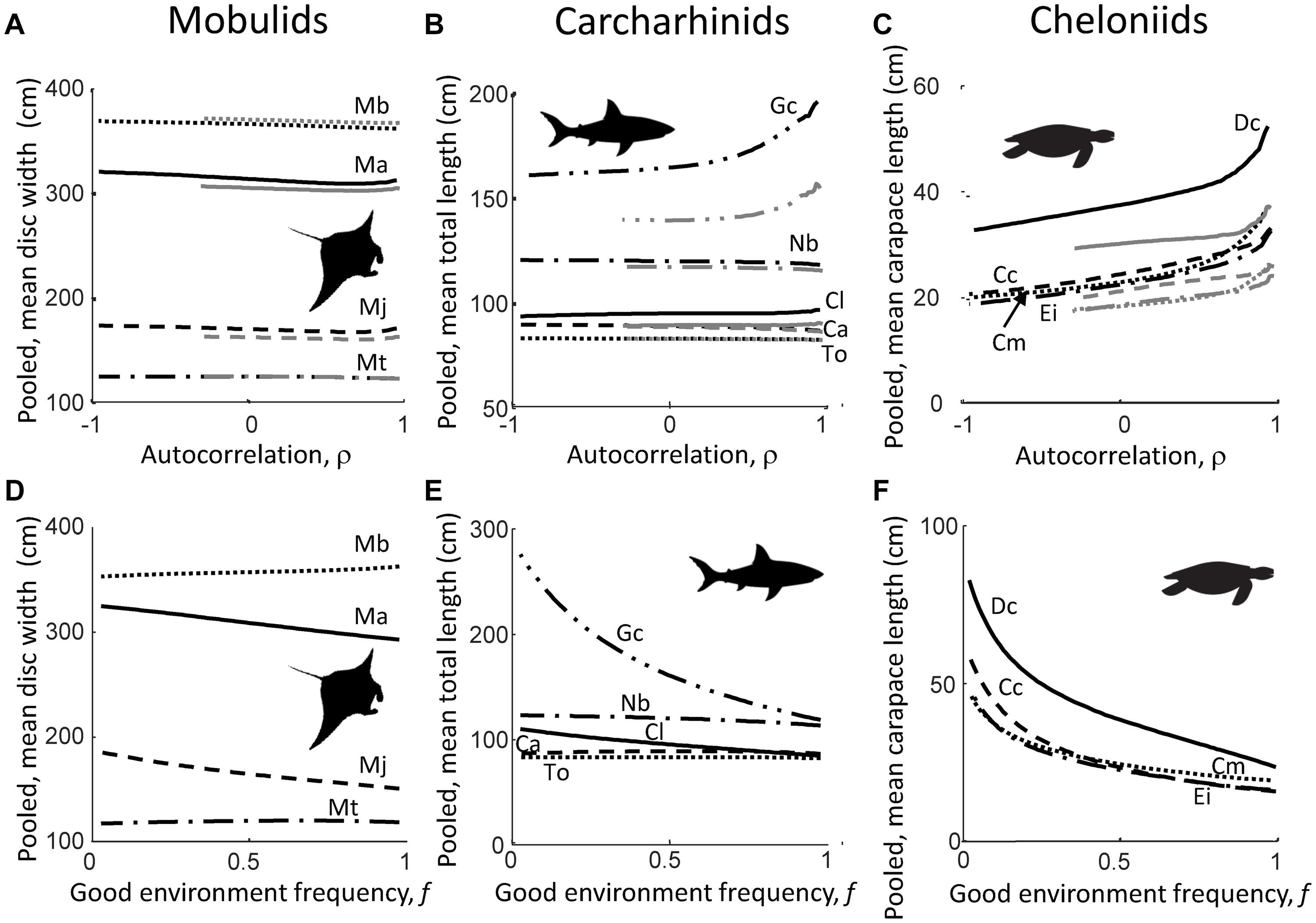
Figure 2. Shifts in pooled mean body size across the gradient of environmental autocorrelation ρ (A–C), and across the gradient of good environment frequency f ranging from almost zero to almost unity (D,E), for mobulids (A,D), carcharhinids (B,E), and cheloniids (C,F). Black lines in (A–C) are pooled, mean body size values when the good environment frequency is fixed at f = 0.5; gray lines when f = 0.75. Mobulid species are M. alfredi (Ma; solid lines), M. birostris (Mb; dotted lines), M. japonica (Mj; dashed lines), and M. thurstoni (Mj; dash-dot lines); carcharhinid species are C. limbatus (Cl; solid lines), T. obesus (To; dotted lines), C. amblyrhynchos (Ca; dashed lines), N. brevirostris (Nb; dash-dot lines), and G. cuvier (Gc; dash-dot-dot lines); cheloniid species are D. coriacea (Dc; solid lines), C. mydas (Cm; dotted lines), C. caretta (Cc; dashed lines), and E. imbricatea (Ei; dash-dot lines). Note difference in y-scale between panels.

Elasticity of log(λ_s) to Perturbation of Life History Parameters Across Stochastic Environments

The perturbation analyses revealed which life history parameter elicited relatively the highest change in the log stochastic population growth rate, log(λ_s), within a single stochastic environment. Four parameters influenced log(λ_s) most: an increase (or decrease) in length at puberty, L_p, decreased (or increased) log(λ_s); an increase (or decrease) in maximum length, L_m, increased (or decreased) log(λ_s); an increase (or decrease) in juvenile mortality rate, μ_j, decreased (or increased) log(λ_s); and an increase (or decrease) in the von Bertalanffy growth rate, ${\stackrel{.}{r}}_{\text{B}}$, increased (or decreased) log(λ_s).

Along the environmental autocorrelation gradient of ρ, while keeping good environment frequency, f, fixed at f = 0.5, log(λ_s) was predominantly most sensitive to perturbation of maximum length, L_m, across the mobulid species (Table 3). Exceptions were log(λ_s) of the reef manta ray M. alfredi, which was most sensitive to perturbation of length at puberty L_p, and log(λ_s) of the bentfin devil ray M. thurstoni, which was most sensitive to perturbation of L_p at the most negative values of ρ (Table 3). Carcharhinid log(λ_s) was, across species, most sensitive to perturbation of either L_p or L_m across the ρ gradient (Table 3). Cheloniid log(λ_s) was across most of the ρ gradient most sensitive to perturbation of L_p and L_m, but also to perturbation of juvenile mortality rate μ_i and von Bertalanffy growth rate ${\stackrel{.}{r}}_{\text{B}}$, depending on species and ρ value (Table 3).

TABLE 3

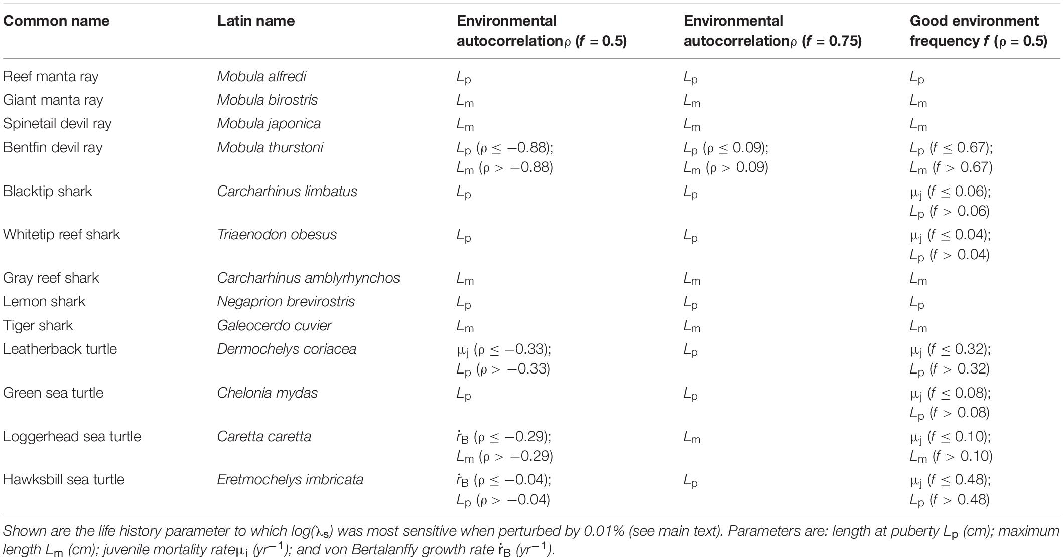
Table 3. The elasticity of the log stochastic population growth rate, log(λ_s), to perturbation of life history parameters across the environmental autocorrelation gradient ρ and across the good environment frequency f.

Running the same perturbation analyses across the environmental autocorrelation gradient ρ, but with the good environment frequency f fixed at f = 0.75, showed that the sensitivity response of mobulid log(λ_s) was very similar to when f = 0.5: mobulids were still mostly sensitive to perturbation of maximum length L_m (Table 3). Exceptions were again M. alfredi and M. thurstoni, for which, at a larger range of negative values of ρ, log(λ_s) is most sensitive to perturbation of length at puberty, L_p. Carcharhinid log(λ_s) was equally sensitive to perturbation of L_p or L_m when f = 0.75 compared to when f = 0.5 (Table 3). Finally, cheloniid log(λ_s) showed the largest difference in sensitivity response across the environmental autocorrelation ρ gradient, depending on whether f = 0.5 or f = 0.75. When f = 0.75, none of the cheloniids log(λ_s) were sensitive to perturbation of juvenile mortality rate μ_i, or the von Bertalanffy growth rate ${\stackrel{.}{r}}_{\text{B}}$; instead, log(λ_s) was always sensitive to perturbation of length at puberty L_p, except for the loggerhead turtle, C. caretta, which log(λ_s) was always most sensitive to perturbation of maximum length L_m (Table 3).

Running the perturbation analyses across the gradient of good environment frequency, f (while keeping environmental autocorrelation ρ = 0) revealed that log(λ_s) showed strikingly similar patterns in elasticity to perturbation of life history parameters as observed across the ρ gradient, with f kept constant at f = 0.5 (Table 3). Specifically, each mobulid log(λ_s) was most sensitive to perturbation of the same life history parameter as observed across the environmental autocorrelation ρ gradient (with f = 0.5; Table 3). The higher values of M. thurstoni log(λ_s) were also mostly sensitive to perturbation of maximum length, L_m, at higher values of f (log(λ_s) was also most sensitive to perturbation of maximum length, L_m, at higher ρ values, with f fixed at f = 0.5; Table 3). For each carcharhinid species, log(λ_s) was mostly sensitive to perturbation of the same life history parameter as observed across the environmental autocorrelation ρ gradient (with f = 0.5; Table 3), with some small differences. At very low good environment frequency f values, log(λ_s) of the blacktip shark C. limbatus and whitetip reef shark T. obesus were most sensitive to perturbation of juvenile mortality rate, μ_i, instead of length at puberty, L_p, at the most negative ρ values (Table 3). Finally, cheloniid log(λ_s) was again most sensitive to perturbation of L_p, L_m or μ_i, but not ${\stackrel{.}{r}}_{\text{B}}$ (as across the ρ gradient with f = 0.5: Table 3), as loggerhead turtle C. caretta and hawksbill turtle E. imbricata log(λ_s) were most sensitive to perturbation of μ_i at low values of f (as opposed to ${\stackrel{.}{r}}_{\text{B}}$ along the lowest range of the ρ gradient with f = 0.5; Table 3).

Linking Life History Parameters to log(λ_s) Across Stochastic Environments

The difference in the log stochastic population growth rate, log(λ_s), between environmental autocorrelation ρ = 1 and ρ = −1 (Figure 1) decreased significantly with increasing scaled, maximum reproduction rate R_m, both when good environment frequency f = 0.5 and when f = 0.75 (Figures 3B,E). There was no significant relationship between the difference in log(λ_s) at ρ = 1 and ρ = −1 and juvenile mortality rate μ_j (Figures 3A,D) or scaled von Bertalanffy growth rate, ${\stackrel{.}{r}}_{\text{B}}$ (Figures 3C,F). In contrast, the difference in log(λ_s) between f = 1 and f = 0 increased significantly with increasing juvenile mortality rate μ_i (Figure 3G), showed a non-significant, positive trend with increasing scaled, maximum reproduction rate R_m (Figure 3H), and increased significantly with increasing, scaled von Bertalanffy growth rate, ${\stackrel{.}{r}}_{\text{B}}$ (Figure 3I). Adult mortality rate μ_a did not significantly relate to the difference in log(λ_s) at ρ = 1 and ρ = −1 with f = 0.50 ($\widehat{e}$ = −0.01; p = 0.98; R² < 0.01), to the difference in log(λ_s) at ρ = 1 and ρ = −1 with f = 0.75 ($\widehat{e}$ = −0.001; p = 0.97; R² < 0.01), and to the difference in log(λ_s) between f = 1 and f = 0 ($\widehat{e}$ = 3.06; p = 0.30; R² = 0.10).

FIGURE 3

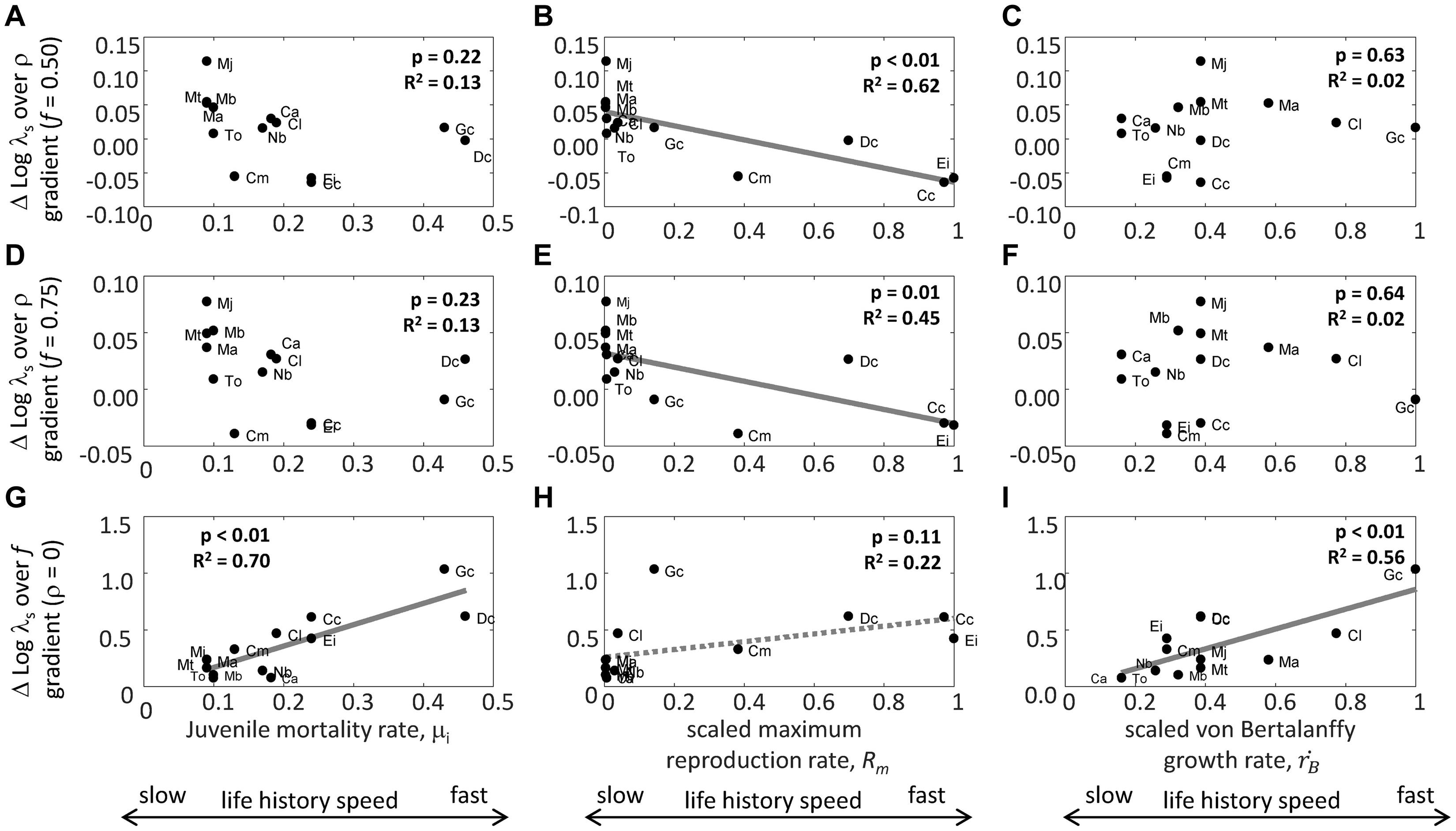
Figure 3. Relationship between juvenile mortality rate, μ_i (yr^–1) (A,D,G), scaled maximum reproduction rate R_m (# yr^–1), (B,E,H), scaled von Bertalanffy growth rate, ${\stackrel{.}{r}}_B$ (yr^–1), (C,F,I) and the difference between the log stochastic population growth rate, log(λ_s), at the end and beginning of the environmental autocorrelation ρ gradient with good environment frequency f = 0.50 (A–C), the difference between log(λ_s) at the end and beginning of the environmental autocorrelation ρ gradient with f = 0.75, (D–F), and the difference between log(λ_s) at the end and beginning of the good environment frequency f gradient (with ρ = 0; G–I). P-values and R² values are indicated for each relationship in each panel, with significant relationships plotted (note: H indicates a non-significant trend). Abbreviations are Mobulid species M. alfredi (Ma), M. birostris (Mb), M. japonica (Mj), and M. thurstoni (Mj); carcharhinid species C. limbatus (Cl), T. obesus (To), C. amblyrhynchos (Ca), N. brevirostris (Nb), and G. cuvier (Gc); and cheloniid species D. coriacea (Dc), C. mydas (Cm), C. caretta (Cc), and E. imbricatea (Ei). The relationship between μ_i, R_m and ${\stackrel{.}{r}}_B$ and the fast-slow life history speed continuum is indicated.

Discussion

Our goal was to assess whether the effects of environmental autocorrelation and good environment frequency on a select group of marine megafauna demography can be predicted from the life history traits that comprise each species’ life history strategy. We found that responses in how the log stochastic population growth rate, log(λ_s), varied across the environmental autocorrelation and good environment frequency gradients were grossly captured by variation in three life history traits: juvenile mortality rate, (scaled) maximum reproduction rate and von Bertalanffy growth rate. Higher values of these traits are characteristic of faster life histories, whereas lower values of these traits are characteristic of slower life histories (Gaillard et al., 2016; Salguero-Gómez et al., 2016). Along this mortality-reproduction axis of life history speed we found that the turtles, the blacktip shark and the tiger shark displayed a higher increase in log(λ_s) with increasing good environment frequency than the other sharks and the rays. Across the environmental autocorrelation gradient from blue to red noise, we found that log(λ_s) of the turtles and the tiger shark decreased, whereas log(λ_s) of the other sharks and the rays increased in similar magnitude across the same gradient.

Are There General Life History Patterns Across Stochastic Environments?

Changes in the patterning of environmental stochasticity (Table 1) may have significant implications for population viability worldwide (Heino and Sabadell, 2003; Ruokolainen et al., 2009; Fey and Wieczynski, 2016). It is thus urgent to gain an in-depth understanding of the life history processes that result in distinct population responses between slow and fast life histories to shifts in environmental stochasticity. The conventional approach to do so partitions variation in life history statistics used to describe both ecological and evolutionary dynamics – like generation time, age at maturity and mean lifetime reproductive success – across many species along an axis of life history speed and an axis of reproductive strategy (Stearns, 1989, Gaillard et al., 2016; Salguero-Gómez et al., 2016; Paniw et al., 2018; Capdevila et al., 2020). A population’s position in this 2D life history space is then taken to inform on its response to environmental change. This conventional approach is phenomenological and lacks a mechanistic representation of the biological processes that give rise to the observed variation in life history statistics (Musick, 1999; Salguero-Gómez, 2017; Salguero-Gómez et al., 2018). Instead, we used a recently developed functional trait approach where the demographic processes of growth and reproduction are described mechanistically by individual energy budgets (Smallegange et al., 2017). Because the model is constructed from (functional) life history traits, we were able to directly relate variation in life history traits to the demographic consequences of shifts in environmental stochasticity.

Unsurprisingly, we found that, as the good environment frequency increased, the log stochastic population growth rate, log(λ_s), of all species increased, although species at the slow end of our mortality-reproduction axis of life history speed (predominantly the rays) showed a lower increase than the species at the fast end of the life history speed axis (particularly the turtles, blacktip shark, and tiger shark). We surmise that this difference in response is predominantly due to differences in reproduction rates between the slower and faster life history strategies. The faster life histories have relatively high maximum reproduction rates (R_m). Because for non-starving adults, reproduction is proportional to the product of expected feeding level E(Y) and R_m (Eq. 6), an increase in the frequency of high E(Y) has a proportionally larger effect on population growth of fast life histories than that of slow ones. This effect is reflected in the response of pooled, mean body size across the gradient of good environment frequency. Whereas pooled, mean body size of the slower life histories showed at most a slight, steady decline across this gradient, pooled, mean body size of the faster life histories decreased greatly with increasing good environment frequency. The latter shift in population size-structure reflects a substantial, relative increase in the proportion of small (juvenile) individuals compared to large (adult) ones, and thus an increase in reproduction, in line with the relatively strong increase in log(λ_s) over this gradient. Despite the fact that pooled, mean body size decreased with increasing good environment frequency, it should be noted that the largest size that an individual can attain, L_∞ (Kooijman, 2010), will increase because it is positively related with feeding level following the relationship L_∞ = L_m.E(Y) (Smallegange et al., 2017).

A more surprising finding was that, over the environmental autocorrelation gradient from blue (high, negative values of ρ) to red noise (high, positive values of ρ), log(λ_s) of the faster life histories decreased in value, whereas log(λ_s) of the slower life histories increased in value of similar magnitude. This result is surprising because it contrasts with the result that Paniw et al. (2018) found, in which log(λ_s) of faster life histories changed in absolute value more over the environmental autocorrelation gradient from white to red noise than log(λ_s) of slower species. The latter pattern is in line with empirical and theoretical findings (Franco and Silvertown, 2004; Morris et al., 2008, 2011; Salguero-Gómez et al., 2016), whereas the pattern that we found is not. One reason could be that the taxa that we studied differ in their life history traits in ways that do not fit the typical pace-of-life axis of variation in life history strategy that has emerged from large(r), cross-taxonomical studies on animals and plants (Gaillard et al., 1989; Salguero-Gómez et al., 2016; Paniw et al., 2018), including aquatic species (Cortés, 2002; Frisk et al., 2005; Quetglas et al., 2016; Capdevila et al., 2020). Specifically, the fast-slow life history strategy continuum is bounded by the fast-living end where species develop quickly, have high reproduction rates, but also high mortality rates, and the slow-living end where species develop slowly, have low reproduction rate, but also low mortality rates (Stearns, 1992). Following this characterization, empirical and theoretical findings have shown that slow life history species are typically less sensitive to environmental autocorrelation than fast life history species, precisely because they are long-lived (Franco and Silvertown, 2004; Salguero-Gómez et al., 2016), have long generation times (Tuljapurkar et al., 2009), and low juvenile and adult mortality rates (Morris et al., 2008, 2011). The slower life history species in our study indeed have lower mortality rates than the faster species, but all the species that we studied are long-lived with long generation times. It is perhaps this atypical combination of life history traits that marine megafauna display that underlies the contrasting demographic responses to environmental autocorrelation of the slower and faster life histories, which, in our study, are characterized by low, respectively, high juvenile mortality and reproduction. The next step is thus to mechanistically understand how temporal stochasticity in environmental conditions drives these contrasting demographic responses between the turtles and tiger shark on the one hand, and the rays and other sharks the other hand.

In response to a shift from blue to red environmental autocorrelation, log(λ_s) of all rays showed the highest increase in value, whereas log(λ_s) of the turtles and the tiger shark showed the highest decrease in value. The turtles and the tiger shark have in common that they have very high juvenile mortality rates, higher than those of the rays. Additionally, the turtles show by far the greatest leap in growth from hatchling to length at puberty. All of this means that any prolonged period of unfavorable environmental conditions, which occurred either half the time (f = 0.5) or a quarter of the time (f = 0.75) under the red noise environments we investigated, have high negative impact on juvenile persistence in these species. Long periods of unfavorable environmental conditions slow individual growth (Eqn 6), prolonging the period over which juveniles are exposed to high mortality until they reach their size at puberty. As a result, fewer will survive as adults to reproduce, lowering log(λ_s). This process is reflected in the population size-structure: pooled, mean body size of the turtles and tiger shark increased over the environmental autocorrelation gradient as log(λ_s) decreased, reflecting reduced reproduction and proportional decrease of smaller sized individuals. The rays, in contrast, appeared to profit from the prolonged periods of favorable conditions under red noise, judging from the increase in log(λ_s) and corresponding slight decline in pooled, mean body size (due to increased reproduction) across the environmental autocorrelation gradient from blue to red. These results provide a fresh perspective onto the theoretical prediction that populations that recover slowly from past perturbations [like long-lived [iteroparous] species in constant environments (Salguero-Gómez et al., 2016)] should be more sensitive to environmental autocorrelation than those that are more resilient (Tuljapurkar and Haridas, 2006). Our finding that long-lived marine megafauna are sensitive to environmental autocorrelation, coupled with the fact that a similar functional trait analysis revealed that the manta ray M. alfredi was more sensitive to environmental autocorrelation than the fast life history amphipod O. gammarellus (Smallegange and Berg, 2019), are in line with the latter theoretical prediction. Conventional approaches, however, have found that population persistence of long-lived animal and plant species in autocorrelated environments is buffered from environmental variation, and, crucially, this patterns was independent of reproductive strategy (e.g., Metcalf and Koons, 2007; Morris et al., 2008). Yet, we find that it is precisely the reproductive strategy of marine megafauna that plays such an important role in their demographic responses, because it determines whether populations grow or decline over the environmental autocorrelation gradient in environmental conditions. The finding by Paniw et al. (2018) that fast life histories were on average more sensitive to environmental autocorrelation than slow species explained 50% of the variance in sensitivity to environmental autocorrelation. Perhaps the remaining variation is unexplained because not all species (groups) strictly map onto the fast-slow life history continuum (this study; Jongejans et al., 2010; McDonald et al., 2017). Finding general life history patterns in how species respond to environmental change is important as it aids our prediction of population persistence, extinction, and diversification (Salguero-Gómez et al., 2016), particularly in the absence of species-specific information in case of many marine organisms (Heppell et al., 1999). However, we should not lose sight of the fact that general life history patterns are not always expected (Galipaud and Kokko, in press), in which case it can be crucial to mechanistically understand how specific interactions between environmental conditions and life history traits drive a population’s response to environmental autocorrelation.

Some Implications for Assessing the Impact of Environmental Change on Marine Megafauna Persistence

The global demand for marine animal products such as shark fins (Clarke et al., 2006), swim bladders (Sadovy and Cheung, 2003; Clarke, 2004), and ray gill plates (White et al., 2006; Ward-Paige et al., 2013) is unsustainable (Berkes et al., 2006; Lenzen et al., 2012). Particularly for the slower life history species has the intense fishing exploitation that targets these demands resulted in population declines and increased risks of extinction, sometimes with synergistic effects of environmental conditions (Jennings et al., 1999; Schindler et al., 2002). Assessing how responses to environmental change of species with contrasting life history strategies differ within an ecological community is thus essential to manage mixed fisheries (Musick, 1999; Jennings and Rice, 2011; Link, 2013). Scholars of chondrichthyans – cartilaginous fishes including rays and sharks – often use the maximum intrinsic rate of population increase, r_max, to assess a population’s status. When population trajectories are lacking, which is often the case for oceanic species (Bradshaw et al., 2007), r_max can be a useful statistic to evaluate a species’ relative risk of overexploitation by fishing (Dulvy et al., 2014) as it can be taken as the equivalent of the fishing mortality that drives a species to extinction (Myers and Mertz, 1998). The statistic r_max is estimated by solving the Euler–Lotka equation (Myers and Mertz, 1998), the most simple versions of which take survival and reproduction schedules as input parameters (Stearns, 1992). Like the Euler–Lotka equation (Stearns, 1992), a DEB-IPM is parameterized by survival and reproduction rates, but also takes the von Bertalanffy growth rate and three length parameters as input (Smallegange et al., 2017). However, whereas the Euler–Lotka equation assumes density-independence (Stearns, 1992), a DEB-IPM can account for density-dependence, either simulated via the expected feeding level E(Y), or incorporated mechanistically by including resource dynamics (Smallegange et al., 2017). Many applications of the Euler–Lotka equation to chondrichthyan demographic responses to environmental perturbations set survival to maturity close to unity (García et al., 2008; Hutchings et al., 2012; Dulvy et al., 2014, but see Pardo et al., 2016a, b), assuming very high juvenile survival rates because chondrichthyans invest highly into offspring. Yet even within this group of species, reproductive strategies can differ greatly (Branstetter, 1990). Our analysis using the DEB-IPM warns against assuming high juvenile survival across chondrichthyans, because the different reproductive strategies of at least some carcharhinids sharks and mobulid rays can result in markedly different demographic responses to environmental change.

Our perturbation analyses revealed that the log stochastic population growth rate, log(λ_s), of all marine megafauna that we studied was, across most, if not all of the length of each stochastic gradient, most sensitive to perturbation of length at puberty, L_p, or maximum length, L_m. Because we took a life history approach, we can examine how a change in either parameter affects population performance. A decrease in L_p, all else being equal, means that individuals start reproducing at a smaller size (Kooijman and Metz, 1984), but they may also produce fewer or smaller offspring (Hume, 2019). In rays and sharks, a decrease in size at maturity can reduce fecundity, because smaller mothers produce smaller offspring (Sibly et al., 2018; Hume, 2019), which have been postulated to have lower fitness (Motta et al., 2007; Hume, 2019). However, in, e.g., the lemon shark, smaller juveniles have higher survival rates than larger individuals of the same age, which could favor maturation at a smaller size (Dibattista et al., 2007). Additionally, several conspecific sea turtle populations differ in length at puberty (Goshe et al., 2010; Bell and Pike, 2012; Snover et al., 2013; Avens et al., 2015, 2017, 2020; Marn et al., 2019). To investigate how the interaction between the benefits and costs of maturing at a smaller size affects population growth rates, we re-ran all our analyses for a scenario in which length at puberty of all cheloniid species is increased by 10% or decreased by 10% (Supplementary Appendix). We found that our results are robust against perturbation of length at puberty, because increasing or decreasing length at puberty of sea turtles by 10% did not qualitatively affect how different life history traits are linked to population responses to shifts in environmental stochasticity (Supplementary Appendix). The other parameter that log(λ_s) was very sensitive to was maximum length, L_m. A decrease in L_m will result in smaller individuals within a population (Eqn 4). Smaller individuals lay fewer eggs (because R_m is related to L_m (Smallegange et al., 2017: Supplementary Appendix) so that a decrease in L_m can reduce population size. In the marine environment, a decrease in L_m can be caused by the selective (over)fishing of large individuals, because prolonged (over)fishing of the largest individuals can impose selection on the developmental processes underlying growth and development and drive contemporary evolutionary responses in L_p and L_m toward earlier maturation at smaller sizes (Waples and Audzijonyte, 2016). In many fishes, selective (over)fishing has reduced mean body size (Frisk et al., 2005; Fenberg and Roy, 2008). For example, mean body size of whale sharks Rhincodon typus has declined in response to fishing, and, at the same time, population abundance has reduced (Bradshaw et al., 2009). These observations, in concert with our findings, signify the importance of understanding the eco-evolutionary interaction between (evolutionary) shifts in life history traits and population growth to be able to better predict population responses of marine megafauna to fishing and environmental change.

Conclusion and Outlook

We found that, across a range of mobulid, carcharhinid and cheloniid species, faster life histories were more sensitive to temporal frequency of good environment conditions, but both faster and slower life histories were equally sensitive, although of opposite sign, to environmental autocorrelation. These patterns are atypical, likely following from the unusual life history traits that these megafauna display. Our analysis is a first exploration of marine megafaunal life history strategies across stochastic environments. As such, we did not take into account specifics of the different species life histories, although our post hoc perturbation of length at puberty of sea turtles did not qualitatively affect how marine megafaunal life history traits are linked to shifts in environmental stochasticity (Supplementary Appendix). Most sea turtles undergo a major ontogenetic habitat shift between oceanic and neritic foraging areas (Ramirez et al., 2015, 2017; Tomaszewicz et al., 2017, 2018). The disconnect and timing of occupation of different feeding habitats could have an impact on sea turtle population responses to shifts in environmental stochasticity. Observed changes in marine systems due to climate change include shifts in range and changes in algal, plankton and fish abundances (Intergovernmental Panel on Climate Change [IPCC], 2007), thus affecting food availability (Hamann et al., 2013) and potentially the environmental autocorrelation of food availability over time, or the frequency with which food availability is favorable (good environment frequency). Because such climate-induced changes can impact population responses to harvesting (Isomaa et al., 2014; Smallegange and Ens, 2018), future work should focus on understanding the impact of shifting environmental stochasticity on (harvested) populations (Huntingford et al., 2013; Boulton and Lenton, 2015). Other shifts in environmental stochasticity are associated with sea temperature. For example, the Pacific Decadal Oscillation and North Pacific sea surface temperatures have become more red-shifted in the period from 1900 to 2015 (Huntingford et al., 2013; Boulton and Lenton, 2015). The reddening of such climate variability entails that populations experience prolonged periods of potentially favorable conditions, but most likely also of unfavorable, more extreme conditions (van der Bolt et al., 2018). Prolonged periods of high temperate can skew sex ratios in sea turtles (Spotila et al., 1987), reduce hatchling survival (Spotila and Standora, 1985; Matsuzawa et al., 2002; Glen et al., 2003; Godfrey and Mrosovsky, 2006), and reduce nesting and feeding habitats due to increasing frequency of storms associated with high sea surface temperature (Hawkes et al., 2009; Pike and Stiner, 2007; Pike et al., 2015). More elaborate, species-specific DEB models that include effects of temperature (e.g., Marn et al., 2017a, b, 2019; Stubbs et al., 2020) could form the basis to explore in detail how populations respond to such environmental change. All in all, our findings signify the importance of understanding how life history traits and population responses to environmental change are linked. Such understanding is a basis for accurate predictions of marine megafauna population responses to environmental perturbations like (over)fishing, and to shifts in the autocorrelation of environmental variables, ultimately contributing toward bending the curve on marine biodiversity loss.

Data Availability Statement

The datasets generated in this study can be found in online repositories. The names of the repository/repositories and accession number(s) can be found below: https://doi.org/10.6084/m9.figshare.12738749.

Author Contributions

IS conceived of the project and took the lead in design, coordination, and writing. All authors brought distinctive expertise to the collaboration and contributed importantly to the ideas represented, as well as through the drafting and revising of the manuscript.

Funding

IS acknowledges funding from the Netherlands Organisation for Scientific Research (VIDI grant no. 864.13.005).

Conflict of Interest

The authors declare that the research was conducted in the absence of any commercial or financial relationships that could be construed as a potential conflict of interest.

Acknowledgments

We thank Anieke van Leeuwen and two reviewers for valuable comments on an earlier version of this manuscript.

Supplementary Material

The Supplementary Material for this article can be found online at: https://www.frontiersin.org/articles/10.3389/fmars.2020.597492/full#supplementary-material

References

Add-my-pet (2020). Database of Code, Data and DEB Model Parameters. Available at: https://www.bio.vu.nl/deb/deblab/add_my_pet/index_main.html (accessed October 9, 2020).

Google Scholar

Ariño, A., and Pimm, S. L. (1995). On the nature of population extremes. Evol. Ecol. 9, 429–443. doi: 10.1007/bf01237765

CrossRef Full Text | Google Scholar

Avens, L., Goshe, L. R., Coggins, L., Shaver, D. J., Higgins, B., and Landry, A. M. Jr., et al. (2017). Variability in age and size at maturation, reproductive longevity, and long-term growth dynamics for Kemp’s ridley sea turtles in the Gulf of Mexico. PLoS One 12:e0173999. doi: 10.1371/journal.pone.0173999

PubMed Abstract | CrossRef Full Text | Google Scholar

Avens, L., Goshe, L. R., Coggins, L., Snover, M. L., Pajuelo, M., Bjorndal, K. A., et al. (2015). Age and size at maturation and adult stage duration for loggerhead sea turtles in the western North Atlantic. Mar. Biol. 162, 1749–1767. doi: 10.1007/s00227-015-2705-x

CrossRef Full Text | Google Scholar

Avens, L., Goshe, L. R., Zug, G. R., Balaze, G. H., Benson, S. R., and Harris, H. (2020). Regional comparison of leatherback sea turtle maturation attributes and reproductive longevity. Mar. Biol. 167:4.

Google Scholar

Bakker, E. S., Pagès, J. F., Arthur, R., and Alcoverro, T. (2016). Assessing the role of large herbivores in the structuring and functioning of freshwater and marine angiosperm ecosystems. Ecography 39, 162–179. doi: 10.1111/ecog.01651

CrossRef Full Text | Google Scholar

Balazs, G. H., and Chaloupka, M. (2004). Spatial and temporal variability in somatic growth of green sea turtles (Chelonia mydas) resident in the Hawaiian Archipelago. Mar. Biol. 145, 1043–1059. doi: 10.1007/s00227-004-1387-6

CrossRef Full Text | Google Scholar

Bell, I., and Pike, D. A. (2012). Somatic growth rates of hawksbill turtles Eretmochelys imbricata in a northern Great Barrier Reef foraging area. Mar. Ecol. Prog. Ser. 446, 275–283. doi: 10.3354/meps09481

CrossRef Full Text | Google Scholar

Berkes, F., Hughes, T. P., Steneck, R. S., Wilson, J. A., Bellwood, D. R., and Crona, B. (2006). Globalization, roving bandits, and marine resources. Science 311, 1557–1558. doi: 10.1126/science.1122804

PubMed Abstract | CrossRef Full Text | Google Scholar

Boulton, C. A., and Lenton, T. M. (2015). Slowing down of North Pacific climate variability and its implications for abrupt ecosystem change. Proc. Natl Acad. Sci.U.S.A. 112, 11496–11501. doi: 10.1073/pnas.1501781112

PubMed Abstract | CrossRef Full Text | Google Scholar

Bradshaw, C. J. A., Fitzpatrick, B. M., Steinberg, C. C., Brook, B. W., and Meekan, M. G. (2009). Decline in whale shark size and abundance at Ningaloo Reef over the past decade: the world’s largest fish is getting smaller. Biol. Conserv. 141, 1894–1905. doi: 10.1016/j.biocon.2008.05.007

CrossRef Full Text | Google Scholar

Bradshaw, C. J. A., Mollet, H. F., and Meekan, M. G. (2007). Inferring population trends for the world’s largest fish from mark–recapture estimates of survival. J. Anim. Ecol. 76, 480–489. doi: 10.1111/j.1365-2656.2006.01201.x

PubMed Abstract | CrossRef Full Text | Google Scholar

Branstetter, S. (1987). Age and growth estimates for blacktip, Carcharhinus limbatus, and spinner, C. brevipinna, sharks from the Northwestern Gulf of Mexico. Copeia 4, 964–974. doi: 10.2307/1445560

CrossRef Full Text | Google Scholar

Branstetter, S. (1990). “Early life-history implications of selected carcharhinoid and lamnoid sharks of the northwest Atlantic,” in Elasmobranchs as Living Resources: Advances in the Biology Ecology Systematics and the Status of the Fisheries NOAA Technical Report NMFS 90, Vol. 90, eds H. L. J. Pratt, S. H. Gruber, and T. Taniuchi (NOAA), 17–28.

Google Scholar

Broderick, A. C., Glen, F., Godley, B. J., and Hays, G. C. (2003). Variation in reproductive output of marine turtles. J. Exp. Mar. Biol. Ecol. 288, 95–109. doi: 10.1016/s0022-0981(03)00003-0

CrossRef Full Text | Google Scholar

Brooks, E. J., Sims, D. W., Danylchuk, A. J., and Sloman, K. A. (2013). Seasonal abundance, philopatry and demographic structure of Caribbean reef shark (Carcharhinus perezi) assemblages in the north-east Exuma Sound, The Bahamas. Mar. Biol. 160, 2535–2546. doi: 10.1007/s00227-013-2246-0

CrossRef Full Text | Google Scholar

Byrne, M. E., Vaudo, J. J., Harvey, G. C. M. N., Johnston, W., Wetherbee, B. M., and Shivji, M. (2019). Behavioral response of a mobile marine predator to environmental variables differs across ecoregions. Ecography 42, 1569–1578. doi: 10.1111/ecog.04463

CrossRef Full Text | Google Scholar

Capdevila, P., Beger, M., Blomberg, S. P., Hereu, B., Linares, C., and Salguero-Gómez, R. (2020). Longevity, body dimension and reproductive mode drive differences in aquatic versus terrestrial life history strategies. Funct. Ecol. 34, 1613–1625. doi: 10.1111/1365-2435.13604

CrossRef Full Text | Google Scholar

Carlson, J. K., Sulikowski, J. R., and Baremore, I. E. (2006). Do differences in life history exist for blacktip sharks, Carcharhinus limbatus, from the United States South Atlantic Bight and Eastern Gulf of Mexico? Environ. Biol. Fish. 77, 279–292. doi: 10.1007/s10641-006-9129-x

CrossRef Full Text | Google Scholar

Carr, A. F., Carr, M. H., and Meylan, A. B. (1978). The ecology and migrations of sea turtles. 7, the West Caribbean green turtle colony. Bull. AMNH 162:1.

Google Scholar

Casale, P., Mazaris, A. D., and Freggi, D. (2011). Estimation of age at maturity of loggerhead sea turtles Caretta caretta in the Mediterranean using length-frequency data. Endanger. Spec. Res. 13, 123–129. doi: 10.3354/esr00319

CrossRef Full Text | Google Scholar

Casale, P., Nicolosi, P., Freggi, D., Turchetto, M., and Argano, R. (2003). Leatherback turtles (Dermochelys coriacea) in Italy and in the Mediterranean basin. Herpetol. J. 13, 135–140.

Google Scholar

Caswell, H. (2001). Matrix Population Models. Sunderland, MA: Sinauer Associates.

Google Scholar

Chaloupka, M., and Limpus, C. (2005). Estimates of sex- and age-class-specific survival probabilities for a southern Great Barrier Reef green sea turtle population. Mar. Biol. 146, 1251–1261. doi: 10.1007/s00227-004-1512-6

CrossRef Full Text | Google Scholar

Chaloupka, M. Y., and Limpus, C. J. (1997). Robust statistical modelling of hawksbill sea turtle growth rates (southern Great Barrier Reef). Mar. Ecol. Prog. Ser. 146, 1–8. doi: 10.3354/meps146001

CrossRef Full Text | Google Scholar

Clarke, S. C. (2004). Understanding pressures on fishery resources through trade statistics: a pilot study of four products in the Chinese dried seafood market. Fish Fish. 5:5374.

Google Scholar

Clarke, S. C., McAllister, M. K., Milner-Gulland, E. J., Kirkwood, G. P., Michielsens, C., Agnew, D. J., et al. (2006). Global estimates of shark catches using trade records from commercial markets. Ecol. Lett. 9, 1115–1126. doi: 10.1111/j.1461-0248.2006.00968.x

PubMed Abstract | CrossRef Full Text | Google Scholar

Clements, C., and Ozgul, A. (2016). Including trait-based early warning signals helps predict population collapse. Nat. Commun. 7:10984.

Google Scholar

Compagno, L. J. V. (1984). FAO Species Catalogue. Vol. 4. Sharks of the world. An Annotated and Illustrated Catalogue of Shark Species Known to Date. Part 2 - Carcharhiniformes. FAO Fish. Synop. 125(4/2):251-655. Rome: FAO.

Google Scholar

Cortés, E. (2002). Incorporating uncertainty into demographic modeling: application to shark populations and their conservation. Conserv. Biol. 16, 1048–1062. doi: 10.1046/j.1523-1739.2002.00423.x

CrossRef Full Text | Google Scholar

Coulson, T. (2012). Integral projections models, their construction and use in posing hypotheses in ecology. Oikos 121, 1337–1350. doi: 10.1111/j.1600-0706.2012.00035.x

CrossRef Full Text | Google Scholar

Dalgleish, H. J., Koons, D. N., and Adler, P. B. (2010). Can life history traits predict the response of forb populations to changes in climate variability? J. Anim. Ecol. 98, 209–217. doi: 10.1111/j.1365-2745.2009.01585.x

CrossRef Full Text | Google Scholar

Davenport, J. (1997). Temperature and the life-history strategies of sea turtles. J. Thermal Biol. 22, 479–488. doi: 10.1016/s0306-4565(97)00066-1

CrossRef Full Text | Google Scholar

Davidson, A. D., Boyer, A. G., Kim, H., Pompa-Mansilla, S., Hamilton, M. J., Costa, D. P., et al. (2012). Drivers and hotspots of extinction risk in marine mammals. Proc. Natl. Acad. Sci. U.S.A. 109, 3395–3400. doi: 10.1073/pnas.1121469109

PubMed Abstract | CrossRef Full Text | Google Scholar

deRoos, A. M., and Persson, L. (2013). Population and Community Ecology of Ontogenetic Development (Monographs in Population Biology, 51). Princeton, NJ: Princeton University Press.

Google Scholar

Dibattista, J. D., Feldheim, K. A., Gruber, S. H., and Hendry, A. P. (2007). When bigger is not better: selection against large size, high condition and fast growth in juvenile lemon sharks. J. Evol. Biol. 20, 201–212. doi: 10.1111/j.1420-9101.2006.01210.x

PubMed Abstract | CrossRef Full Text | Google Scholar

Duffy, C. A. J., and Abbott, D. (2003). Sightings of mobulid rays from northern New Zealand, with confirmation of the occurrence of Manta birostris in New Zealand waters. N. Z. J. Mar. Freshwat. Res. 37, 715–721. doi: 10.1080/00288330.2003.9517201

CrossRef Full Text | Google Scholar

Dulvy, N. K., Pardo, S. A., Simpfendorfer, C. A., and Carlson, J. K. (2014). Diagnosing the dangerous demography of manta rays using life history theory. PeerJ 2:e400. doi: 10.7717/peerj.400

PubMed Abstract | CrossRef Full Text | Google Scholar

Dutton, D. L., Dutton, P. H., Chaloupka, M., and Boulon, R. H. (2005). Increase of a Carribean leather back turtle Dermochelys coriacea nesting population linked to long-term nest protection. Biol. Cons. 126, 186–194. doi: 10.1016/j.biocon.2005.05.013

CrossRef Full Text | Google Scholar

Dwyer, R. G., Krueck, N. C., Udyawer, V., Heupel, M. R., Chapman, D., Pratt, H. L., et al. (2020). Individual and population benefits of marine reserves for reef sharks. Curr. Biol. 30, 480–489. doi: 10.1016/j.cub.2019.12.005

PubMed Abstract | CrossRef Full Text | Google Scholar

Easterling, M. R., Ellner, S. P., and Dixon, P. M. (2000). Size-specific sensitivity: applying a new structured population model. Ecology 81, 694–708. doi: 10.1890/0012-9658(2000)081[0694:sssaan]2.0.co;2

CrossRef Full Text | Google Scholar

Eguchi, T., Dutton, P. H., Garner, S. A., and Alexander-Garner, J. (2006). “Estimating juvenile survival rates and age at first nesting of leatherback turtles at St. Croix, US Virgin Islands,” in Proceedings of the 26th Annual Symposium on Sea Turtle Biology and Conservation (Miami, FL: U.S. Department of Commerce. NOAA Technical Memorandum NMFS-SEFSC).

Google Scholar

Estes, J., Terborgh, J., Brashares, J., Power, M., Berger, J., Bond, W., et al. (2011). Trophic downgrading of planet earth. Science 333, 301–306.

Google Scholar

Fenberg, P. B., and Roy, K. (2008). Ecological & evolutionary consequences of size-selective harvesting: how much do we know? Mol. Ecol. 17, 209–220.

Google Scholar

Ferretti, F., Worm, B., Britten, G. L., Heithaus, M. R., and Lotze, H. K. (2010). Patterns and ecosystem consequences of shark declines in the ocean. Ecol. Lett. 13, 1055–1071.

Google Scholar

Fey, S. B., and Wieczynski, D. J. (2016). The temporal structure of the environment may influence range expansions during climate warming. Glob. Change Biol. 23, 635–645. doi: 10.1111/gcb.13468

PubMed Abstract | CrossRef Full Text | Google Scholar

Franco, M., and Silvertown, J. (1996). Life history variation in plants: an exploration of the fast-slow continuum hypothesis. Phil. Trans. R. Soc. B 351, 1341–1348. doi: 10.1098/rstb.1996.0117

CrossRef Full Text | Google Scholar

Franco, M., and Silvertown, J. (2004). A comparative demography of plants based upon elasticities of vital rates. Ecology 85, 531–538. doi: 10.1890/02-0651

CrossRef Full Text | Google Scholar

Frazer, N. B. (1986). Survival from egg to adulthood in a declining population of loggerhead turtles, Caretta caretta. Herpetologica 42, 47–55.

Google Scholar

Frazer, N. B., and Ehrhart, L. M. (1985). Preliminary growth models for green, Chelonia mydas, and loggerhead, Caretta caretta, turtles in the wild. Copeia 1, 73–79. doi: 10.2307/1444792

CrossRef Full Text | Google Scholar

Freitas, R. H. A., Rosa, R. S., Gruber, S. H., and Wetherbee, B. M. (2006). Early growth and juvenile population structure of lemon sharks, Negaprion brevirostris, in the Atol das Rocas Biological Reserve, off north-east Brazil. J. Fish Biol. 68, 1319–1332. doi: 10.1111/j.0022-1112.2006.00999.x

CrossRef Full Text | Google Scholar

Frisk, M. G., Miller, T. J., and Dulvy, N. K. (2005). Life histories & vulnerability to exploitation of elasmobranchs: inferences from elasticity, perturbation & phylogenetic analyses. J. Northwest Atlantic Fish. Sci. 35, 27–45.

Google Scholar

Gaillard, J.-M., Lemâitre, J. F., Berger, V., Bonenfant, C., Devillard, S., Douhard, M., et al. (2016). “Life histories, axes of variation,” in Encyclopedia of Evolutionary Biology, Vol. 2, ed. R. M. Kliman (Cambridge, MA: Academic Press), 312–323. doi: 10.1016/b978-0-12-800049-6.00085-8

CrossRef Full Text | Google Scholar

Gaillard, J. -M., Pontier, D., Allainé, D., Lebreton, J. D., Trouvilliez, J., Clobert, J., et al. (1989). An analysis of demographic tactics in birds and mammals. Oikos 56, 59–76. doi: 10.2307/3566088

CrossRef Full Text | Google Scholar

Galipaud, M., and Kokko, H. (in press). Adaptation, and plasticity in life-history theory: how to derive predictions. Evol. Hum. Behav. doi: 10.1016/j.evolhumbehav.2020.06.007

CrossRef Full Text | Google Scholar

García, V. B., Lucifora, L. O., and Myers, R. A. (2008). The importance of habitat and life history to extinction risk in sharks, skates, rays and chimaeras. Proc. R. Soc. B 275, 83–89. doi: 10.1098/rspb.2007.1295

PubMed Abstract | CrossRef Full Text | Google Scholar

García-Carreras, B., and Reuman, D. C. (2011). An empirical link between the spectral colour of climate and the spectral colour of field populations in the context of climate change. J. Anim. Ecol. 80, 1042–1048. doi: 10.1111/j.1365-2656.2011.01833.x

PubMed Abstract | CrossRef Full Text | Google Scholar

Getz, W. M., and Haight, R. G. (1989). Population Harvesting: Demographic Models of Fish, Forest, and Animal Resources. Princeton, NJ: Princeton University Press.

Google Scholar

Glen, F., Broderick, A. C., Godley, B. J., and Hays, G. C. (2003). Incubation environment affects phenotype of naturally incubated green turtle hatchlings. J. Mar. Biol. Assoc. U.K 83, 1183–1186. doi: 10.1017/s0025315403008464h

CrossRef Full Text | Google Scholar

Godfrey, M. H., and Mrosovsky, N. (2006). Pivotal temperature for green sea turtles, Chelonia mydas, nesting in Suriname. Herpetol. J. 16, 55–61.

Google Scholar

Goshe, L. R., Avens, L., Scharf, F. S., and Southwood, A. L. (2010). Estimation of age at maturation and growth of Atlantic green turtles (Chelonia mydas) using skeletochronology. Mar. Biol. 157, 1725–1740. doi: 10.1007/s00227-010-1446-0

CrossRef Full Text | Google Scholar

Halley, J. M. (1996). Ecology, evolution and 1/f-noise. Trends Ecol. Evol. 52, 91–100.

Google Scholar

Hamann, M., Fuentes, M. M. P. B., Ban, N. C., and Mocellin, V. J. L. (2013). “Climate change and marine turtles,” in The Biology of Sea Turtles, Vol. III, eds J. Wyneken, K. J. Lohmann, and J. A. Musick (Boca Raton, FL: CRC Press), 353–397. doi: 10.1201/b13895-14

CrossRef Full Text | Google Scholar

Hammerschlag, N., Skubel, R. A., Sulikowski, J., Irschick, D. J., and Gallagher, A. J. (2018). A comparison of reproductive and energetic states in a marine apex predator (the tiger shark, Galeocerdo cuvier). Physiol. Biochem. Zool. 91, 933–942. doi: 10.1086/698496

PubMed Abstract | CrossRef Full Text | Google Scholar

Hawkes, L. A., Broderick, A. C., Godfrey, M. H., and Godley, B. J. (2009). Climate change and marine turtles. Endange. Spec. Res. 7, 137–154. doi: 10.3354/esr00198

CrossRef Full Text | Google Scholar

Heino, M., and Sabadell, M. (2003). Influence of coloured noise on the extinction risk in structured population models. Biol. Conserv. 110, 315–325. doi: 10.1016/s0006-3207(02)00235-5

CrossRef Full Text | Google Scholar

Heppell, S. S., Crowder, L. B., and Menzel, T. R. (1999). “Life table analysis of long-lived marine species with implications for conservation and management,” in Proceedings of the Symposium Conservation of Long-Lived Marine Animals on Life in the Slow Lane: Ecology and Conservation of Long-Lived Marine Animals, ed. J. A. Musick (Monterey, CA), 137–148.

Google Scholar

Heppell, S. S., Crowder, L. B., and Crouse, D. T. (1996a). Models to evaluate headstarting as a management tool for long-lived turtles. Ecol. Appl. 6, 556–565. doi: 10.2307/2269391

CrossRef Full Text | Google Scholar

Heppell, S. S., Limpus, C. J., Crouse, D. T., Frazer, N. B., and Crowder, L. B. (1996b). Population model analysis for the loggerhead sea turtle, Caretta caretta, in Queensland. Wildlife Res. 23, 143–159. doi: 10.1071/wr9960143

CrossRef Full Text | Google Scholar

Hirth, H. F. (1980). Some aspects of the nesting behaviour and reproductive biology of marine turtles. Am. Zool. 20, 507–523. doi: 10.1093/icb/20.3.507

PubMed Abstract | CrossRef Full Text | Google Scholar

Hirth, H. F., and Schaffer, W. (1974). Survival rates of the green turtle, Chelonia mydas, necessary to maintain stable populations. Copeia 1974, 544–546. doi: 10.2307/1442553

CrossRef Full Text | Google Scholar

Hume, J. B. (2019). Higher temperatures increase developmental rate & reduce body size at hatching in the small-eyed skate Raja microocellata: implications for exploitation of an elasmobranch in warming seas. Fish Biol. 95, 655–658. doi: 10.1111/jfb.13997

PubMed Abstract | CrossRef Full Text | Google Scholar

Huntingford, C., Jones, P. D., Livina, V. N., Lenton, T. M., and Cox, P. M. (2013). No increase in global temperature variability despite changing regional patterns. Nature 500, 327–330. doi: 10.1038/nature12310

PubMed Abstract | CrossRef Full Text | Google Scholar

Hutchings, J. A., Myers, R. A., García, V. B., Lucifora, L. O., and Kuparinen, A. (2012). Life-history correlates of extinction risk and recovery potential. Ecol. Appl. 22, 1061–1067. doi: 10.1890/11-1313.1

CrossRef Full Text | Google Scholar

Inchausti P, and Halley, J. M. (2002). The long-term variability and spectral colour of animal populations. Evol. Ecol. Res. 4, 1–16.

Google Scholar

Intergovernmental Panel on Climate Change [IPCC] (2007). “Summary for policymakers,” in Climate Change 2007: Climate Change Impacts, Adaptation, and Vulnerability. Contribution of Working Group II to the Fourth Assessment Report of the Intergovernmental Panel on Climate Change, eds S. Solomon, D. Quin, M. Manning, Z. Chen, M. Marquis, K. B. Averyt, et al. (Cambridge: Cambridge University Press). doi: 10.18772/22008034792.11

CrossRef Full Text | Google Scholar

Isomaa, M., Kaitala, V., and Laakso, J. (2014). Precautionary management of Baltic Sea cod (Gadus morhua callarias) under different environmental noise and harvesting strategies. Boreal Environ. Res. 19, 39–50.

Google Scholar

Janzen, F. J. (1994). Vegetational cover predicts the sex ratio of hatchling turtles in natural nests. Ecology 75, 1593–1599. doi: 10.2307/1939620

CrossRef Full Text | Google Scholar

Jatmiko, I., and Catur Nugroho, S. (2020). Biological and population parameters of tiger Shark Galeocerdo cuvier, landed in Tanjung Luar, West Nusa Tenggara. E3S Web Conf. 147:02010. doi: 10.1051/e3sconf/202014702010

CrossRef Full Text | Google Scholar

Jennings, S., Greenstreet, S. P. R., and Reynolds, J. D. (1999). Structural change in an exploited fish community: a consequence of differential fishing effects on species with contrasting life histories. J. Anim. Ecol. 68, 617–627. doi: 10.1046/j.1365-2656.1999.00312.x

CrossRef Full Text | Google Scholar

Jennings, S., and Rice, J. (2011). Towards an ecosystem approach to fisheries in Europe: a perspective on existing progress and future directions. Fish Fish. 12, 125–137. doi: 10.1111/j.1467-2979.2011.00409.x

CrossRef Full Text | Google Scholar

Jones, T. T. (2009). Energetics of the Leatherback Turtle, Dermochelys Coriacea. PhD thesis. Vancouver: Univ British Columbia.

Google Scholar

Jongejans, E., De Kroon, H., Tuljapurkar, S., and Shea, K. (2010). Plant populations track rather than buffer climate fluctuations. Ecol. Lett. 13, 736–743. doi: 10.1111/j.1461-0248.2010.01470.x

PubMed Abstract | CrossRef Full Text | Google Scholar

Kashiwagi, T. (2014). Conservation Biology and Genetics of the Largest Living Rays: Manta Rays. PhD Thesis. Queensland, QLD: University of Queensland.

Google Scholar

Killam, K. A., and Parsons, G. R. (1989). Age and growth of the blacktip shark, Carcharhinus limbatus, near Tampa Bay, Florida. Fish. Bull. 87, 845–867.

Google Scholar

Kneebone, J., Natanson, L. J., Andrews, A. H., and Howell, W. H. (2008). Using bomb radiocarbon analyses to validate age and growth estimates for the tiger shark, Galeocerdo cuvier, in the western North Atlantic. Mar. Biol. 154, 423–434. doi: 10.1007/s00227-008-0934-y

CrossRef Full Text | Google Scholar

Kooijman, S. A. L. M. (2010). Dynamic Energy Budget Theory for Metabolic Organization. Cambridge: Cambridge University Press.

Google Scholar

Kooijman, S. A. L. M., and Metz, J. A. J. (1984). On the dynamics of chemically stressed populations: the deduction of population consequences from effects on individuals. Ecotoxicol. Environ. Saf. 8, 254–274. doi: 10.1016/0147-6513(84)90029-0

CrossRef Full Text | Google Scholar

Lande, R., Saether, B. -E., and Engen, S. (1997). Threshold harvesting for sustainability of fluctuating resources. Ecology 78, 1341–1350. doi: 10.1890/0012-9658(1997)078[1341:thfsof]2.0.co;2

CrossRef Full Text | Google Scholar

Lenzen, M., Moran, D., Kanemoto, K., Foran, B., Lobefaro, L., and Geschke, A. (2012). International trade drives biodiversity threats in developing nations. Nature 486:109112.

Google Scholar

Limpus, C. J. (1992). The hawksbill turtle, Eretmochelys imbricata, in Queensland: population structure within a southern Great Barrier Reef feeding ground. Wildlife Res. 19, 489–506. doi: 10.1071/wr9920489

CrossRef Full Text | Google Scholar

Limpus, C. J., and Reed, P. C. (1985). Green sea turtles stranded by cyclone Kathy on the south-western coast of the Gulf of Carpentaria. Wildlife Res. 12, 523–533. doi: 10.1071/wr9850523

CrossRef Full Text | Google Scholar

Link, J. S. (2013). Ecosystem approaches to fisheries: a global perspective. Fisheries 38:463. doi: 10.1080/03632415.2013.851556

CrossRef Full Text | Google Scholar

Marn, N., Jusup, M., Catteau, S., Kooijman, S. A. L. M., and Klanjšček, T. (2019). Comparative physiological energetics of Mediterranean and North Atlantic loggerhead turtles. J. Sea Res. 143, 100–118. doi: 10.1016/j.seares.2018.06.010

CrossRef Full Text | Google Scholar

Marn, N., Jusup, M., Legović, T., Kooijman, S. A. L. M., and Klanjšček, T. (2017a). Environmental effects on growth, reproduction, and life-history traits of loggerhead turtles. Ecol. Mod. 360, 163–178. doi: 10.1016/j.ecolmodel.2017.07.001

CrossRef Full Text | Google Scholar

Marn, N., Kooijman, S. A., Jusup, M., and Legović, T. (2017b). Inferring physiological energetics of loggerhead turtle (Caretta caretta) from existing data using a general metabolic theory. Mar. Environ. Res. 126, 14–25. doi: 10.1016/j.marenvres.2017.01.003

PubMed Abstract | CrossRef Full Text | Google Scholar

Marshall, A. D., Kashiwagi, T., Bennett, M. B., Deakos, M., Stevens, G., Mcgregor, F., et al. (2011). Manta Alfredi. The IUCN Red List of Threatened Species. Version 2015.2.

Google Scholar

Matsuzawa, Y., Sato, K., Sakamoto, W., and Bjorndal, K. (2002). Seasonal fluctuations in sand temperature: effects on the incubation period and mortality of loggerhead sea turtle (Caretta caretta) pre-emergent hatchlings in Minabe. Japan. Mar. Biol. 140, 639–646. doi: 10.1007/s00227-001-0724-2

CrossRef Full Text | Google Scholar

McDonald, J. L., Franco, M., Townley, S., Ezard, T. H., Jelbert, K., and Hodgson, D. J. (2017). Divergent demographic strategies of plants in variable environments. Nat. Ecol. Evol. 1:29.

Google Scholar

Merow, C., Dahlgren, J. P., Metcalf, C. J. E., Childs, D. Z., Evans, M. E. K., Jongejans, E., et al. (2014). Advancing population ecology with integral projection models: a practical guide. Methods Ecol. Evol. 5, 99–110. doi: 10.1111/2041-210x.12146

CrossRef Full Text | Google Scholar

Metcalf, C. J. E., and Koons, D. N. (2007). Environmental uncertainty, autocorrelation and the evolution of survival. Proc. R. Soc B 274, 2153–2160. doi: 10.1098/rspb.2007.0561

PubMed Abstract | CrossRef Full Text | Google Scholar

Meyer, C. G., O’Malley, J. M., Papastamatiou, Y. P., Dale, J. J., Hutchinson, M. R., Anderson, J. M., et al. (2014). Growth and maximum size of tiger sharks (Galeocerdo cuvier) in Hawaii. PLoS One 9:e84799. doi: 10.1371/journal.pone.0084799

PubMed Abstract | CrossRef Full Text | Google Scholar

Miller, J. D. (1997). “Reproduction in sea turtles,” in The Biology of Sea Turtles, eds P. L. Lutz and J. A. Musick (Boca Rato, FL: CRC Press), 51–82.

Google Scholar

Moffitt, S. E., Moffitt, R. A., Sauthoff, W., Davis, C. V., Hewett, K., and Hill, T. M. (2015). Paleoceanographic insights on recent oxygen minimum zone expansion: lessons for modern oceanography. PLoS One 1:e0115246. doi: 10.1371/journal.pone.0115246

PubMed Abstract | CrossRef Full Text | Google Scholar

Morreale, S. J., Ruiz, G. J., and Standora, E. (1982). Temperature-dependent sex determination: current practices threaten conservation of sea turtles. Science 216, 1245–1247. doi: 10.1126/science.7079758

PubMed Abstract | CrossRef Full Text | Google Scholar

Morris, W. F., Altmann, J., Brockman, D. K., Cords, M., Fedigan, L. M., Pusey, A. E., et al. (2011). Low demographic variability in wild primate populations: fitness impacts of variation, covariation, and serial correlation in vital rates. Am. Natural. 177, E14–E28.

Google Scholar

Morris, W. F., Pfister, C. A., Tuljapurkar, S., Haridas, C. V., Boggs, C. L., Boyce, M. S., et al. (2008). Longevity can buffer plant and animal populations against changing climatic variability. Ecology 89, 19–25. doi: 10.1890/07-0774.1

CrossRef Full Text | Google Scholar

Motta, F. S., Namora, R. C., Gadig, O. B. F., and Braga, F. M. S. (2007). Reproductive biology of the Brazilian sharpnose shark (Rhizoprionodon lalandii) from southeastern Brazil. ICES J. Mar. Sci. 64, 1829–1835. doi: 10.1093/icesjms/fsm159

CrossRef Full Text | Google Scholar

Mourier, J., Mills, S. C., and Planes, S. (2013). Population structure, spatial distribution and life-history traits of blacktip reef sharks Carcharhinus melanopterus. J. Fish Biol. 82, 979–993. doi: 10.1111/jfb.12039

PubMed Abstract | CrossRef Full Text | Google Scholar

Mourier, J., and Planes, S. (2013). Direct genetic evidence for reproductive philopatry and associated fine-scale migrations in female blacktip reef sharks (Carcharhinus melanopterus) in French Polynesia. Mol. Ecol. 22, 201–214. doi: 10.1111/mec.12103

PubMed Abstract | CrossRef Full Text | Google Scholar

Musick, J. A. (1999). “Life in the slow lane: ecology and conservation of long-lived marine animals,” in Proceedings of the Symposium Conservation of Long-Lived Marine Animals, Monterey, CA.

Google Scholar

Myers, R. A., and Mertz, G. (1998). The limits of exploitation: a precautionary approach. Ecol. Appl. 8, 165–169.

Google Scholar

Oh, B. Z. L., Sequeira, A. M. M., Meekan, M. G., Ruppert, J. L. W., and Meeuwig, J. J. (2017). Predicting occurrence of juvenile shark habitat to improve conservation planning. Conserv. Biol. 31, 635–645. doi: 10.1111/cobi.12868

PubMed Abstract | CrossRef Full Text | Google Scholar

Paleczny, M., Hammill, E., Karpouzi, V., and Pauly, D. (2010). Population trend of the world’s monitored seabirds, 1950–2010. PLoS One 10:e0129342. doi: 10.1371/journal.pone.0129342

PubMed Abstract | CrossRef Full Text | Google Scholar

Paniw, M., Ozgul, A., and Salguero-Gómez, R. (2018). Interactive life-history traits predict sensitivity of plants and animals to temporal autocorrelation. Ecol. Lett. 21, 275–286. doi: 10.1111/ele.12892

PubMed Abstract | CrossRef Full Text | Google Scholar

Pardo, S. A., Kindsvater, H. K., Cuevas-Zimbrón, E., Soso-Nishizaki, O., Pérez-Jímenez, J. C., and Dulvy, N. K. (2016a). Growth, productivity, and relative extinction risk of a data-sparse devil ray. Sci. Rep. 6:33745.

Google Scholar

Pardo, S. A., Kindsvater, H. K., Reynolds, J. D., and Dulvy, N. K. (2016b). Maximum intrinsic rate of population increase in sharks, rays, and chimaeras: the importance of survival to maturity. Can. J. Fish. Aqu. Sci. 73, 1159–1163. doi: 10.1139/cjfas-2016-0069

CrossRef Full Text | Google Scholar

Pike, D. A., Roznik, E. A., and Bell, I. (2015). Nest inundation from sea-level rise threatens sea turtle population viability. R. Soc. Open Sci. 2:150127. doi: 10.1098/rsos.150127

PubMed Abstract | CrossRef Full Text | Google Scholar

Pike, D. A., and Stiner, J. C. (2007). Sea turtle species vary in their susceptibility to tropical cyclones. Oecologia 153, 471–478. doi: 10.1007/s00442-007-0732-0

PubMed Abstract | CrossRef Full Text | Google Scholar

Price, E. R., Wallace, B. P., Reina, R. D., Spotila, J. R., Paladino, F. V., Piedra, R., et al. (2006). Size, growth, and reproductive output of adult female leatherback turtles Dermochelys coriacea. Endanger. Spec. Res. 1, 41–48. doi: 10.3354/esr001041

CrossRef Full Text | Google Scholar

Quetglas, A., Rueda, L., Alvares-Berastegui, D., Guijarro, B., and Massutí, E. (2016). Contrasting responses to harvesting and environmental drivers of fast and slow life history species. PLoS One 11:e0148770. doi: 10.1371/journal.pone.0148770

PubMed Abstract | CrossRef Full Text | Google Scholar

Rambahiniarison, J. M., Lamoste, M. J., Rohner, C. A., Murray, R., Snow, S., Labaja, J., et al. (2018). Life history, growth, and reproductive biology of four mobulid species in the Bohol Sea, Philippines. Front. Mar. Sci. 5:269. doi: 10.3389/fmars.2018.00269

CrossRef Full Text | Google Scholar

Ramirez, M. D., Avens, L., Seminoff, J. A., Goshe, L. R., and Heppell, S. S. (2015). Patterns of loggerhead turtle ontogenetic shifts revealed through isotopic analysis of annual skeletal growth increments. Ecosphere 6, 1–17.

Google Scholar

Ramirez, M. D., Avens, L., Seminoff, J. A., Goshe, L. R., and Heppell, S. S. (2017). Growth dynamics of juvenile loggerhead sea turtles undergoing an ontogenetic habitat shift. Oecologia 183, 1087–1099. doi: 10.1007/s00442-017-3832-5

PubMed Abstract | CrossRef Full Text | Google Scholar

Randhawa, H. S., Poulin, R., and Krkošek, M. (2015). Increasing rate of species discovery in sharks coincides with sharp population declines: implications for biodiversity. Ecography 38, 96–107. doi: 10.1111/ecog.00793

CrossRef Full Text | Google Scholar

Richardson, J. I., Bell, R., and Richardson, T. H. (1999). Population ecology and demographic Implications drawn from an 11-year study of nesting Hawksbill turtles, Eretmochelys imbricata, at Jumby Bay, Long Island, Antigua, West Indies. Chelonian Conserv. Biol. 3, 244–250.

Google Scholar

Robbins, W. D. (2006). Abundance, Demography and Population Structure of the Grey Reef Shark (Carcharhinus amblyrhynchos) and The White Tip Reef Shark (Triaenodon obesus) (Fam. Charcharhinidae). PhD thesis. Douglas QLD: James Cook University.

Google Scholar

Roff, G., Doropoulos, C., Rogers, A., Bozec, Y. M., Krueck, N. C., Aurellado, E., et al. (2016). The ecological role of sharks on coral reefs. Trends Ecol. Evol. 31, 395–407.

Google Scholar

Ruokolainen, L., Linden, A., Kaitala, V., and Fowler, M. S. (2009). Ecological and evolutionary dynamics under coloured environmental variation. Trends Ecol. Evol. 24, 555–563. doi: 10.1016/j.tree.2009.04.009

PubMed Abstract | CrossRef Full Text | Google Scholar

Sadovy, Y., and Cheung, W. L. (2003). Near extinction of a highly fecund fish: the one that nearly got away. Fish Fish. 4:8699.

Google Scholar

Salguero-Gómez, R. (2017). Applications of the fast–slow continuum and reproductive strategy framework of plant life histories. New Phytol. 213, 1618–1624. doi: 10.1111/nph.14289

PubMed Abstract | CrossRef Full Text | Google Scholar

Salguero-Gómez, R., Jones, O. R., Jongejans, E., Blomberg, S. P., Hodgson, D. J., Mbeau-Ache, C., et al. (2016). Fast–slow continuum and reproductive strategies structure plant life-history variation worldwide. Proc. Natl Acad. Sci. U.S.A. 113, 230–235. doi: 10.1073/pnas.1506215112

PubMed Abstract | CrossRef Full Text | Google Scholar

Salguero-Gómez, R., Violle, C., Gimenez, O., and Childs, D. (2018). Delivering the promises of trait-based approaches to the needs of demographic approaches, and vice versa. Funct. Ecol. 32, 1424–1435.

Google Scholar

Schindler, D. E., Essington, T. E., Kitchell, J. F., Boggs, C., and Hilborn, R. (2002). Sharks and tunas: fisheries impacts on predators with contrasting life histories. Ecol. Appl. 12, 735–748. doi: 10.1890/1051-0761(2002)012[0735:satfio]2.0.co;2

CrossRef Full Text | Google Scholar

Schneider, W. (1990). FAO Species Identification Sheets for Fishery Purposes. Field Guide to the Commercial Marine Resources of the Gulf of Guinea. Rome: FAO.

Google Scholar

Sibly, R. M., Kodric-Brown, A., Luna, S. M., and Brown, J. H. (2018). The shark-tuna dichotomy: why tuna lay tiny eggs but sharks produce large offspring. R. Soc. Open Sci. 5:180453. doi: 10.1098/rsos.180453

PubMed Abstract | CrossRef Full Text | Google Scholar

Smallegange, I. M., and Berg, M. (2019). A functional trait approach to identifying life history patterns in stochastic environments. Ecol. Evol. 9, 9350–9361. doi: 10.1002/ece3.5485

PubMed Abstract | CrossRef Full Text | Google Scholar

Smallegange, I. M., Caswell, H., Toorians, M. E. M., and de Roos, A. M. (2017). Mechanistic description of population dynamics using dynamic energy budget theory incorporated into integral projection models. Methods Ecol. Evol. 8, 146–154. doi: 10.1111/2041-210x.12675

CrossRef Full Text | Google Scholar

Smallegange, I. M., and Coulson, T. (2013). Towards a general, population-level understanding of eco-evolutionary change. Trends Ecol. Evol. 28, 143–148. doi: 10.1016/j.tree.2012.07.021

PubMed Abstract | CrossRef Full Text | Google Scholar

Smallegange, I. M., Deere, J. A., and Coulson, T. (2014). Correlative changes in life-history variables in response to environmental change in a model organism. Am. Nat. 183, 784–797. doi: 10.1086/675817

PubMed Abstract | CrossRef Full Text | Google Scholar

Smallegange, I. M., and Ens, H. M. (2018). Trait-based predictions and responses from laboratory mite populations to harvesting in stochastic environments. J. Anim. Ecol. 87, 893–905. doi: 10.1111/1365-2656.12802

PubMed Abstract | CrossRef Full Text | Google Scholar

Smallegange, I. M., van der Ouderaa, I. B. C., and Tibiriçá, Y. (2016). Effects of yearling, juvenile and adult survival on reef manta ray (Manta alfredi) demography. PeerJ 4:e2370. doi: 10.7717/peerj.2370

PubMed Abstract | CrossRef Full Text | Google Scholar

Snover, M. L., Balazs, G. H., Murakawa, S. K. K., Hargrove, M. R. R., and Seitz, W. A. (2013). Age and growth rates of Hawaiian hawksbill turtles (Eretmochelys imbricata) using skeletochronology. Mar. Biol. 160, 37–46. doi: 10.1007/s00227-012-2058-7

CrossRef Full Text | Google Scholar

Sousa, T., Domingos, T., Poggiale, J. C., and Kooijman, S. A. L. M. (2010). Dynamic energy budget theory restores coherence in biology. Philos. Trans. R. Soc. Lond. B Biol. Sci. 365, 3413–3428. doi: 10.1098/rstb.2010.0166

PubMed Abstract | CrossRef Full Text | Google Scholar

Spotila, J. R., and Standora, E. A. (1985). Environmental constraints on the thermal energetics of sea turtles. Copeia 3, 694–702. doi: 10.2307/1444763

CrossRef Full Text | Google Scholar

Spotila, J. R., Standora, E. A., Morreale, S. J., and Ruiz, G. J. (1987). Temperature dependent sex determination in the green turtle (Chelonia mydas): effects on the sex ratio on a natural nesting beach. Herpetologica 43:74.

Google Scholar

Stearns, S. C. (1992). The Evolution of Life Histories. Oxford: Oxford University Press, 247.

Google Scholar

Stubbs, J. L., Marn, N., Vanderklift, M. A., Fossette, S., and Mitchell, N. J. (2020). Simulated growth and reproduction of green turtles (Chelonia mydas) under climate change and marine heatwave scenarios. Ecol. Model. 431:109185. doi: 10.1016/j.ecolmodel.2020.109185

CrossRef Full Text | Google Scholar

Saether, B.-E., Coulson, T., Grøtan, V., Engen, S., Altwegg, R., Armitage, K. B., et al. (2013). How life history influences population dynamics in fluctuating environments. Am. Natural. 182, 743–759. doi: 10.1086/673497

PubMed Abstract | CrossRef Full Text | Google Scholar

Stearns, S. C. (1989). Trade-offs in life-history evolution. Funct. Ecol. 3, 259–268.

Google Scholar

Teh, L. S., Teh, L. C. L., and Jolis, G. (2018). An economic approach to marine megafauna conservation in the coral triangle: marine turtles in Sabah, Malaysia. Mar. Policy 89, 1–10. doi: 10.1016/j.marpol.2017.12.004

CrossRef Full Text | Google Scholar

Tomaszewicz, C. N. T., Seminoff, J. A., Avens, L., Goshe, L. R., Gruez-Baron, J. M., Peckham, S. H., et al. (2018). Expanding the coastal forager paradigm: long-term pelagic habitat use by green turtles Chelonia mydas in the eastern Pacific Ocean. Mar. Ecol. Prog. Ser. 587, 217–234. doi: 10.3354/meps12372

CrossRef Full Text | Google Scholar

Tomaszewicz, C. N. T., Seminoff, J. A., Peckham, S. H., Avens, L., and Kurle, C. M. (2017). Intrapopulation variability in the timing of ontogenetic habitat shifts in sea turtles revealed using δ15N values from bone growth rings. J. Anim. Ecol. 86, 694–704. doi: 10.1111/1365-2656.12618

PubMed Abstract | CrossRef Full Text | Google Scholar

Tuljapurkar, S., Gaillard, J.-M., and Coulson, T. (2009). From stochastic environments to life histories and back. Philos. Trans. R. Soc. B Biol. Sci. 364, 1499–1509. doi: 10.1098/rstb.2009.0021

PubMed Abstract | CrossRef Full Text | Google Scholar

Tuljapurkar, S., and Haridas, C. V. (2006). Temporal autocorrelation and stochastic population growth. Ecol. Lett. 9, 327–337. doi: 10.1111/j.1461-0248.2006.00881.x

PubMed Abstract | CrossRef Full Text | Google Scholar

Tuljapurkar, S., Horvitz, C. C., and Pascarella, J. B. (2003). The many growth rates and elasticities of populations in random environments. Am. Natural. 162, 489–502. doi: 10.1086/378648

PubMed Abstract | CrossRef Full Text | Google Scholar

van Buskirk, J., and Crowder, L. B. (1994). Life-history variation in marine turtles. Copeia 1994, 66–81. doi: 10.2307/1446672

CrossRef Full Text | Google Scholar

van der Bolt, B., van Nes, E. H., Bathiany, S., Vollebregt, M. E., and Scheffer M. (2018). Climate reddening increases the chance of critical transitions. Nat. Clim. Chang. 8, 478–484.

Google Scholar

Vianna, G. M. S., Meekan, M. G., Meeuwig, J. J., and Speed, C. W. (2013). Environmental influences on patterns of vertical movement and site fidelity of grey reef sharks (Carcharhinus amblyrhynchos) at aggregation sites. PLoS One 8:e60331. doi: 10.1371/journal.pone.0060331

PubMed Abstract | CrossRef Full Text | Google Scholar

Waples, R. S., and Audzijonyte, A. (2016). Fishery-induced evolution provides insights into adaptive responses of marine species to climate change. Front. Ecol. Environ. 14:217–224. doi: 10.1002/fee.1264

CrossRef Full Text | Google Scholar

Ward-Paige, C. A., Davis, B., and Worm, B. (2013). Global population trends and human use patterns of Manta and Mobula rays. PLoS One 8:e74835. doi: 10.1371/journal.pone.0074835

PubMed Abstract | CrossRef Full Text | Google Scholar

Ward-Paige, C. A., Mora, C., Lotze, H. K., Pattengill-Semmens, C., McClenachan, L., et al. (2010). Large-scale absence of sharks on reefs in the greater-Caribbean: a footprint of human pressures. PLoS One 5:e11968. doi: 10.1371/journal.pone.0011968

PubMed Abstract | CrossRef Full Text | Google Scholar

Webb, C. T., Hoeting, J. A., Ames, G. M., Pyne, M. I., and Poff, N. L. (2010). A structured and dynamic framework to advance traits-based theory and prediction in ecology. Ecol. Lett. 13, 267–283. doi: 10.1111/j.1461-0248.2010.01444.x

PubMed Abstract | CrossRef Full Text | Google Scholar

Wetherbee, B. M., Crow, G. L., and Lowe, C. G. (1997). Distribution, reproduction and diet of the gray reef shark Carcharhinus amblyrhynchos in Hawaii. Mar. Ecol. Prog. Ser. 151, 181–189. doi: 10.3354/meps151181

CrossRef Full Text | Google Scholar

White, W. T., Giles, J., Dharmadi, D., and Potter, I. C. (2006). Data on the bycatch fishery and reproductive biology of mobulid rays (Myliobatiformes) in Indonesia. Fish. Res. 82, 65–73. doi: 10.1016/j.fishres.2006.08.008

CrossRef Full Text | Google Scholar

Whitney, N. M., and Crow, G. L. (2007). Reproductive biology of the tiger shark (Galeocerdo cuvier) in Hawaii. Mar. Biol. 151, 63–70. doi: 10.1007/s00227-006-0476-0

CrossRef Full Text | Google Scholar

Whitney, N. M., Pyle, R. L., Holland, K. N., and Barcz, J. T. (2012). Movements, reproductive seasonality, and fisheries interactions in the whitetip reef shark (Triaenodon obesus) from community-contributed photographs. Environ. Biol. Fish. 93, 121–136. doi: 10.1007/s10641-011-9897-9

CrossRef Full Text | Google Scholar

Zug, G. R., Kalb, H. J., and Luzar, S. J. (1997). Age and growth in wild kemp’s ridley seaturtle Lepidochelys kempii from skeletochronological data. Biol. Conserv. 80, 261–268. doi: 10.1016/s0006-3207(96)00143-7

CrossRef Full Text | Google Scholar