 Vincent Raoult1*
 Clive N. Trueman2
 Kelsey M. Kingsbury3
 Bronwyn M. Gillanders3
 Matt K. Broadhurst4
 Jane E. Williamson5
 Ivan Nagelkerken3
 David J. Booth6
 Victor Peddemors7
 Lydie I. E. Couturier8Troy F. Gaston1
- 1School of Environmental and Life Sciences, University of Newcastle, Ourimbah, NSW, Australia
- 2Ocean and Earth Science, University of Southampton, Southampton, United Kingdom
- 3Southern Seas Ecology Laboratories, School of Biological Sciences and The Environment Institute, The University of Adelaide, Adelaide, SA, Australia
- 4Fisheries Conservation Technology Unit, National Marine Science Centre, New South Wales Department of Primary Industries, Southern Cross University, Coffs Harbour, NSW, Australia
- 5Department of Biological Sciences, Macquarie University, Sydney, NSW, Australia
- 6School of Life Sciences, University of Technology Sydney, Sydney, NSW, Australia
- 7New South Wales Department of Primary Industries, Sydney Institute of Marine Science, Mosman, NSW, Australia
- 8Univ Brest, IRD, Ifremer, CNRS, LEMAR, Plouzané, France
Determining the geographic range of widely dispersed or migratory marine organisms is notoriously difficult, often requiring considerable costs and typically extensive tagging or exploration programs. While these approaches are accurate and can reveal important information on the species, they are usually conducted on only a small number of individuals and can take years to produce relevant results, so alternative approaches may be preferable. The presence of latitudinal gradients in stable carbon isotope compositions of marine phytoplankton offers a means to quickly determine likely geographic population ranges of species that rely on productivity from these resources. Across sufficiently large spatial and temporal scales, the stable carbon isotopes of large coastal or pelagic marine species should reflect broad geographic patterns of resource use, and could be used to infer geographic ranges of marine populations. Using two methods, one based on a global mechanistic model and the other on targeted low-cost latitudinal sampling of fishes, we demonstrate and compare these stable isotope approaches to determine the core population geography of an apex predator, the great hammerhead (Sphyrna mokarran). Both methods indicated similar geographic ranges and suggested that S. mokarran recorded in south-eastern Australia are likely to be from more northern Australian waters. These approaches could be replicated in other areas where coastlines span predictable geographic gradients in isotope values and be used to determine the core population geography of highly mobile species to inform management decisions.
Introduction
Determining the habitat ranges of mobile species is a key precursor for their effective population management (Hobday et al., 2011). For marine species that migrate across large distances, tagging approaches (photo-identification, passive or active tags) are the most widespread methods used to determine geographic ranges (Queiroz et al., 2019). However, while tagging can provide important spatial information (Queiroz et al., 2019) telemetry tags are expensive and satellite tags can have failure rates approaching 50% (Hofman et al., 2019). Also, tags are not always appropriate for smaller species or those that occur in deeper water. Further, tags usually provide few data points that, while informative for certain applications (e.g., determining if individuals use particular habitats, Barnes et al., 2019) have only recently reached population scales > 1,000 for a few commercially important species, such as Atlantic bluefin tuna (Thunnus thynnus) (Block, 2019). Inter-jurisdictional collaborations can alleviate some of these restrictions for producing population-scale tagging outputs on less valuable species, but for regionally isolated work the approach remains challenging (Sequeira et al., 2019). In addition, because tagging relies on collecting data over long periods (i.e., up to 13 years, Holmes et al., 2014), there are inherent delays in subsequent management applications.
An alternative method that provides information on the past geography of migratory species without the logistical and temporal costs described above involves stable isotope analysis, which can be derived from non-lethal tissue sampling. Specifically, the relative abundance of stable isotopes of carbon and nitrogen in marine animal tissues have been used extensively to infer resource use and to examine trophic interactions (Post, 2002). More recently, stable isotope compositions of tissues have been used to address spatial questions such as identifying ocean basin-scale patterns of resource use (Bird et al., 2018), and even reconstructing individual migration histories from archived samples (Trueman et al., 2019). Stable isotope methods offer a means to determine the geographic ranges of migratory marine organisms over large temporal scales (annual to decadal, depending on preserved tissue types) at relatively low costs ($10s USD per sample compared to $100s to 1000s per acoustic or satellite tag, respectively). Nevertheless, there are some caveats that have hindered wider use of this approach.
Spatial applications of stable isotope tracers require a priori knowledge of the spatial distribution of stable isotope ratios (frequently presented as a spatial model or ‘isoscape,’ West et al., 2009). Constructing isoscape models from geographically referenced samples is logistically challenging, especially in offshore marine environments, and relatively few sample-based, marine isoscape models have been constructed (Revill et al., 2009; St. John Glew et al., 2019). Moreover, isotopic compositions of baseline organisms in marine systems are likely to be spatio-temporally dynamic, especially in temperate regions with broad temperature shifts. Therefore, isoscapes created from single sampling events may not describe isotopic gradients expressed in consumer organisms across seasons.
In pelagic marine environments, phytoplankton δ13C values are primarily influenced by the concentration and isotopic composition of dissolved inorganic carbon, and phytoplankton taxonomy and growth (Rau et al., 1982), which strongly covary with temperature and thus latitude. The isotopic fractionation of carbon during photosynthetic fixation by phytoplankton facilitates developing mechanistic biogeochemical models that predict spatio-temporal variations in oceanic phytoplankton δ13C values with reasonable accuracy and precision (e.g., Magozzi et al., 2017). Mechanistic models predicting δ15N values have also been developed (Somes et al., 2010), and regional foraging models have been designed around this isotope (Madigan et al., 2016). However, there is some uncertainty around trophic correction factors of δ15N values for higher-order predators (Olin et al., 2013). This means that the decision to use either δ15N or δ13C models to construct isoscapes will be system or species dependent. Extending mechanistic models predicting isotopic compositions of primary production to observed isotopic compositions of higher trophic level animals is complex. Such models require assumptions of the isotopic effects associated with trophic discrimination factors and food web structure (Bird et al., 2018).
Consequently, while stable isotope methods are an attractive tool for inferring the spatial ecology of marine consumers, as for all ecological modeling, the confidence placed in any inferences depends on the quality of the reference dataset. The relative differences in reference isotope data produced by mechanistic or sample-driven approaches are not well understood, with both methods suffering from either logistical or theoretical limitations. Mechanistic approaches often target low trophic level organisms (plankton or planktivores) (Magozzi et al., 2017) while sample-driven approaches typically capture higher-order predators (Logan et al., 2020), making the two approaches difficult to compare.
Sample-driven isoscape approaches require relatively intensive sampling efforts and are typically only feasible for studying commercially important taxa such as tunas (e.g., Logan et al., 2020). Species that are only sporadically caught or have low commercial value will rarely justify the sampling efforts needed to construct reliable two-dimensional spatial isotope models. For these species, alternative sample-driven approaches, relying on more easily sampled indicator species to construct a reference dataset may be more appropriate, although creating bespoke isoscape models can be logistically challenging (St. John Glew et al., 2019). Nevertheless, where spatial variation in one or more stable isotopes is largely defined by latitudinal gradients, one-dimensional linear models may be sufficient to identify likely latitudinal foraging. However, it is important to acknowledge that in coastal or neritic waters, latitudinal variation of δ13C values may be overpowered by broader isotopic signatures from sources of productivity like macrophytes or marine plants (Hill et al., 2006; Raoult et al., 2018) and from inshore-offshore gradients (Kopp et al., 2015). This could mean latitudinal influences on δ13C values of coastal organisms are more difficult to detect than in pelagic environments—without extensive sampling to account for the range of coastal influences.
Assuming trophic enrichment of stable isotopes can be corrected mathematically, any relatively sedentary species can be used to construct sample-driven, latitudinal models provided they are collected in large enough numbers from a range of habitats and locations that account for the possible range in coastal influences. In parallel, using a global oceanic biogeochemical reference model grounded with localized regional targeted sampling could help extrapolate patterns to broader areas while validating the accuracy of the mechanistic model, and incorporate some of the uncertainty surrounding coastal influences on marine δ13C values. The result would potentially greatly reduce the cost of creating isoscapes while providing justification for using mechanistic approaches that extend beyond sampling areas.
Here we draw on both sample-driven and mechanistic approaches to generate reference isoscapes to infer regional geographic ranges in a high-trophic level and globally threatened (listed as Critically Endangered; Rigby et al., 2019) migratory marine consumer: the great hammerhead (Sphyrna mokarran). Genetic studies on S. mokarran indicate they perform widespread migrations across territorial waters (Guttridge et al., 2017), which makes identifying their geographic range necessary to prioritize effective conservation areas. Off eastern Australia, S. mokarran is caught by bather-protection gillnets (Sumpton et al., 2011; Broadhurst and Cullis, 2020) and fisheries (Roff et al., 2018) in diminishing relative abundances from Cairns, North Queensland (∼17°S) to Woolongong, New South Wales (NSW) (∼34°S) (Raoult et al., 2019). Their apparent rarity off NSW has led to S. mokarran being regionally listed as Vulnerable (Rigby et al., 2019). However, there is a possibility that NSW waters are not part of the core geographic range for this species, and that much of the population spends most of their lives in more northern waters. Deciphering the predominant habitat range and migration of S. mokarran off south-eastern Australia may facilitate more precise conservation-status assessments. The paucity of catches in NSW waters along with a very high discard mortality (Broadhurst and Cullis, 2020) complicates tagging studies that can address this lack of data, although collections of tissue samples obtained from bather-protection programs are available.
Our objective was to determine the geographic range of S. mokarran off NSW, Australia, using stable isotope data obtained from specimens caught in bather-protection gillnets. We assessed whether captured specimens were residents to this area, or whether their core geographic range was more northern than NSW. Our specific aims were to create and compare isoscapes using (i) a sample-driven approach that relied on targeted fish sampling from local commercial fisheries and on zooplanktivore sampling from coastal reefs and could only examine latitudinal patterns, and (ii) a mechanistic approach using a global biogeochemical model that could examine both longitudinal and latitudinal patterns. As a synthesis, we provide a framework for using similar approaches to determine the geographic ranges of other wide-ranging species.
Materials and Methods
Sampling
Muscle tissue samples were collected from 27 S. mokarran caught as bycatch in bather-protection gillnets deployed off Ballina/Evans Head (28.77° S, 153.60° E to 29.10° S; 153.44° E, n = 25) and Newcastle (31.25° S, 146.92° E, n = 2), NSW during summer and autumn, 2018 (see Broadhurst and Cullis, 2020 for a description of the gear; Figure 1). These muscle samples were the same as those used and described in Raoult et al. (2019).
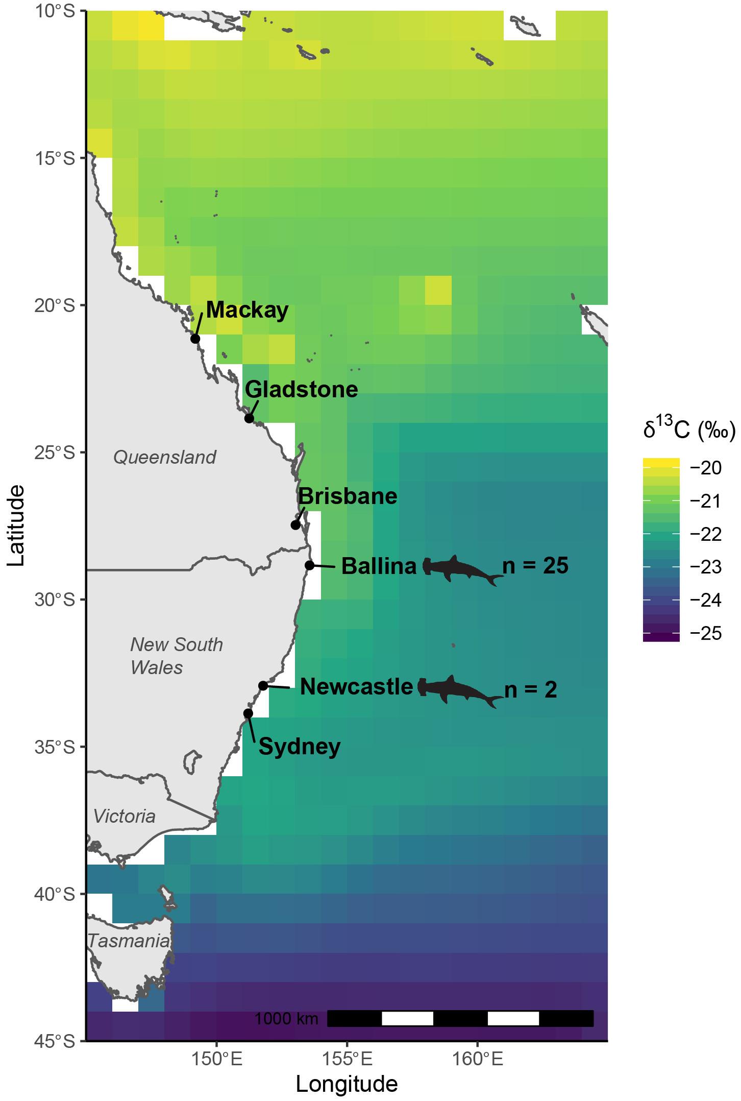
Figure 1. Modeled, biomass-weighted annual median δ13C values of oceanic phytoplankton off eastern Australia per degree of latitude extracted from NEMO-MEDUSA framework, which predicts stable isotope values from modeled sea surface temperature, dissolved inorganic carbon content and isotopic composition and phytoplankton biomass and growth rates. Locations where great hammerhead shark (Sphyrna mokarran) samples were collected are indicated by shark outlines.
Geo-located reference isoscape fish samples were used to constrain latitudinal gradients in consumer δ13C values and were obtained from various sources during austral summers between 2011 and 2018. Fisheries-caught species mostly consisting of fishes but including some cephalopods were purchased directly from fishing co-operatives in January 2018, and only locally landed species (waters adjacent to the fishing co-operative) were included. All operational NSW co-operatives were sampled between Ballina (28.87° S, 153.58° E) and the New South Wales – Victoria border (37.07° S, 149.89° E). Research trawl samples were also obtained off eastern Tasmania (41.25° S, 148.34° E) from the University of Tasmania’s FV Bluefin using a demersal trawl at depths of ∼80 m on the continental shelf in 2016. Reef manta ray (Mobula alfredi) stable isotope values from muscle tissues were obtained from North Stradbroke (27.40° S, 153.53° E) and Lady Elliot islands (24.11° S, 152.71° E) in southern Queensland from Couturier et al. (2013), sampled in 2011 and 2012. Planktivorous reef fishes were captured in a separate juvenile fish survey in 2017 and 2018 from the southern end of the Great Barrier Reef to the New South Wales – Victoria border (Kingsbury et al., 2020). In general, the fishes selected to create the isoscape were considered likely to be feeding from pelagic food webs and were unlikely to be undertaking large annual north/south migrations. Relatively few species were available that fit both criteria, and to create a suitable reference dataset, we sampled across a wide latitudinal range and included a broad range of species at different life history stages. We corrected for potential trophic enrichment effects on δ13C values using the approach outlined below.
Stable Isotope Analysis
Approximately 1-g samples of muscle tissue indicative of yearly resource use (Malpica-Cruz et al., 2013) were extracted from S. mokarran and the fishes obtained from fishing co-operatives and placed onto individual HCl-cleaned glass petri dishes. Samples were dried at 60°C for at least 48 h, then ground into a fine powder using a Retsch MM200 ball mill1. Sphyrna mokarran samples were lipid- and urea-extracted to prevent those components from affecting stable isotope values (Carlisle et al., 2016), as per the methods described in Raoult et al. (2019).
Adjusting Stable Isotope Values for Trophic Enrichment and Lipid Content
High lipid content in muscle tissues can affect δ13C values (Shipley et al., 2017). As a result, all fish samples, excluding lipid and urea-extracted S. mokarran tissues with C:N ratios > 3.5 (indicative of high lipid content), were mathematically corrected using the equation from Post et al. (2007).
Stable isotopes of carbon are typically enriched at higher trophic levels. Since our data comprised various species that were likely feeding at different trophic levels, it was first necessary to correct for confounding effects. To achieve this, we constructed the formula using the widely accepted relationship of enrichment of δ13C values with δ15N values (Caut et al., 2009):
Where δ13Ccorrected is the δ13C value adjusted for trophic enrichment, δ13Cmeasured is the δ13C value from the muscle sample of a fish, δ15Nmeasured is the δ15N value of the same sample, δ15Nmin the lowest δ15N value across all samples in the data set, Δ15N is the 15N diet-tissue discrimination factor for that type of fish, and Δ13C is the 13C the diet-tissue discrimination factor for that same fish. For fishes in this data set, a mean (±SD) Δ15N of 2.5 ± 1.1‰Δ13C of 1.8 ± 1.2‰ was used (Caut et al., 2009). Squid Δ13C of mantle tissue is approximately 0‰ (Hobson and Cherel, 2006), so no transformations were applied. Transformed values that had δ13C values more enriched than −18‰ could indicate possible feeding on benthic algae (Fry et al., 1983; Frédérich et al., 2009; Greenwood et al., 2010; Eurich et al., 2019), however, removing extremes of values would create bias in the following model. To adjust for this, we pre-emptively removed highly enriched δ13C values > −14‰ before analyses.
The δ13Ccorrected values were corrected to the trophic level of a coral reef planktivore, which meant these were still enriched relative to true phytoplankton isotopic values. The difference between exclusive zoo- and phyto-planktivore δ13C values and particulate organic matter (POM) is typically ∼1–2‰ according to planktivore-specific studies (Frédérich et al., 2009; Greenwood et al., 2010). To allow comparison of these results with modeled NEMO-MEDUSA values (see below), all sample-driven δ13Ccorrectedvalues had 1.5‰ subtracted to reflect this plankton-planktivore enrichment.
For S. mokarran, elasmobranch-specific discrimination factors for lipid-extracted muscle were used with a mean (±SD) Δ15N of 2.8 ± 0.3‰ and Δ13C of 1.2 ± 0.4‰ (Hussey et al., 2010). However, there is uncertainty in these values, and diet-tissue discrimination factors are known to affect stable isotope models (Bond and Diamond, 2011). Further, while the sample size of S. mokarran (n = 27) was relatively large for elasmobranch studies, our sampling distribution may not reflect the true distribution of the population. To account for both uncertainty in diet-tissue discrimination factors and population size, we employed a Monte Carlo Markov Chain (MCMC) approach incorporating the variability of the discrimination factors as in Hussey et al. (2010) (0.3‰ for Δ15N and 0.4‰ for Δ13C) to calculate the δ13Ccorrected in the formula above. The distributions of each discrimination factor were modeled assuming a normal distribution with 1,000 samples, and we ran 10,000 simulations. Resulting δ13C values had 1.5‰ subtracted from them to align with the sample-driven data. The result should provide a broad, conservative estimate of the distribution of the δ13C values in the sampled population of S. mokarran.
Modeling Relationships Between Reference δ13C Values and Latitude
We used a general additive model (GAM) framework using the package mgcv (Wood and Wood, 2015) in R to model the relationship between trophic enrichment and lipid-corrected δ13C values in referenced fish and squid data (δ13Cfish) and latitude. We fitted corrected δ13Cfish values as the response variable using a smoothing term with latitude as the predictor and five nodes. This number of nodes was chosen because increases did not significantly improve model fit (R2 increase < 0.05), while creating apparent overfit with nodes at each location where samples were collected. While we did not achieve an empirically ideal model using diagnostic criteria such as estimated degrees of frequency relative to k-values, we are confident that the number of nodes chosen was high enough to detect major trends without over-fitting the model.
Median, biomass-weighted annual modeled phytoplankton δ13C values (δ13Cplk) were generated from NEMO-MEDUSA biogeochemical model output as described in Magozzi et al. (2017), extracting δ13Cplk values from the three degrees of longitude closest to the Australian coastline. Modeled δ13Cplk values were used in a similar fashion as the measured fish and squid reference data. A GAM was used to assess the relationship between modeled δ13Cplk values and latitude. The aim was not only to determine the core geographic range of S. mokarran across a greater latitudinal and longitudinal range, but also to determine whether the mechanistic model aligned with patterns detected in the field-sampled data. Incorporating uncertainty into latitude and longitude bins produced by the mechanistic approach is important to align with the sample-driven technique, however, global models typically have no reliable way of estimating uncertainty (Cooter and Schwede, 2000). To provide a more conservative estimate, we used the mean residual distance of the NEMO-MEDUSA data from the mechanistic GAM for each longitude and latitude bin. Larger confidence intervals would likely only extend the possible area where these sharks would occur, rather than change the geographic center of the area, so this approach is largely insensitive to the chosen confidence interval for this step.
Predicting Sphyrna mokarran Latitudinal Range From Reference Data
Latitudes corresponding to the 1,000 MCMC modeled S. mokarran δ13C values were estimated using the two GAM models linking latitude to δ13Cfish and δ13Cplk values. We partitioned the simulated δ13Cshark data into bins corresponding to 1° latitudinal ranges, where the minimum and maximum δ13C values corresponded to the lower and higher 95% confidence intervals of the GAM produced from the sample-driven reference isoscape (δ13Cfish). The partitioning was such that any given modeled S. mokarranδ13C value could have multiple ‘bins’ where it could occur due to the bin width, thus producing a ‘range’ of possible geographic locations for a single datum. The resulting cumulative counts of the number of modeled sharks assigned to each specific latitude were then transformed into proportions relative to our modeled population. We assumed that likely modeled population peak areas that made up ∼50% of the total population comprised the core habitat for the sampled population.
For both GAM models, multimodal distributions that may occur are assumed to be an artifact of the GAM pattern that can create two or more solutions for one sample depending on the number of nodes. A solution to this problem is to assume the modal peak furthest from the site the animals were caught is the least likely to be the ‘true’ habitat, and to ignore that distribution. Where prior data are available on habitat use of the species (i.e., no use of open ocean/pelagic only and tropical/temperate preference) these can also be used to inform on the validity of the model outputs. These are, of course, open to interpretation, which is why we present the raw model outputs here to highlight that the results of this approach need to be transparent to inspire confidence in the implications.
Cross-Checking of Validity of Models
A risk when producing models on a single study species is that the observed and apparently valid model patterns may be a coincidence brought on by the selected parameters. To determine whether our method could be applied more broadly to other species, we then followed the pattern identical to the above but using data from sharks with habitat distributions inferred from catch data: the southern sawshark (Pristiophorus nudipinnis) and common sawshark (P. cirratus). Both species were combined as ‘ Pristiophorus spp.’ because their fisheries data are not reliably differentiated. These mesopredators are primarily found in south-eastern Australia near Bass Strait (Raoult et al., 2020) and on the coastal shelf and slope. Data from Raoult et al. (2015) (n = 49) were supplemented with other samples obtained from the same trawls used for sample-driven samples (n = 9). For these species we used the diet-tissue discrimination factor of muscle from leopard sharks (Triakis semifasciata), which have a benthic lifestyle similar to Pristiophorus spp., on a fish-based diet from Kim et al. (2012) (Δ15Nof 5.5 ± 0.4‰ and Δ13C of 3.5 ± 0.6‰). Low C:N ratios (<2.5) suggest possible urea impacts. Since urea was not extracted from these tissues, urea is likely depleting δ15N values by ∼0.8‰ (Carlisle et al., 2016). We therefore added 0.8 ± 0.2‰ to δ15N values to compensate and included this uncertainty within the MCMC framework described above. We expected that the core latitude range identified using this approach should broadly align with known habitat distributions, which would provide some clarity as to the ubiquity of the approach.
Results
In total, 681 specimens were used to constrain reference consumer δ13Cfish values and produce a latitudinal relationship (Supplementary Table 1). Modeled δ13Cplk values increased from the south to the north off eastern Australia, with higher values associated with coastal regions north of the New South Wales – Queensland border (Figure 1). This pattern was followed by consistent δ13C values along the NSW coastline, before values rapidly depleted south of the New South Wales – Victoria border.
Descriptive Models of Field-Sampled and Modeled δ13C Values
General additive models summarizing the spatial variation in δ13Cfish values detected a significant effect for the smoothed latitude term (edf = 3.99, F = 2302, p < 0.001) corresponding to higher δ13Cfish values toward the equator. Across the latitudinal gradient, the GAM predicted a break in the positive relationship between latitude and δ13Cfish values between ∼37 and ∼32°S (Figure 2). The deviance explained for this GAM was 29.4%, reflecting the broad distributions of points. The GAM for the mechanistic model δ13Cplk data detected similar effects for the latitudinal smoothing term (edf = 3.98, F = 744, p < 0.001) and the broad pattern agreed approximately with the GAM informed from independent field-sampled consumer δ13Cfish values, with differences in δ13C values generally < 1, and no greater than 1.5 (Supplementary Figure 1). The main differences between the two models was that δ13Cfish values increased dramatically north of 30°S. As expected for outputs from a relatively simple mechanistic model, the GAM explained a high proportion (96.8%) of the deviance in δ13Cplk values with a low mean residual distance of 0.2‰.
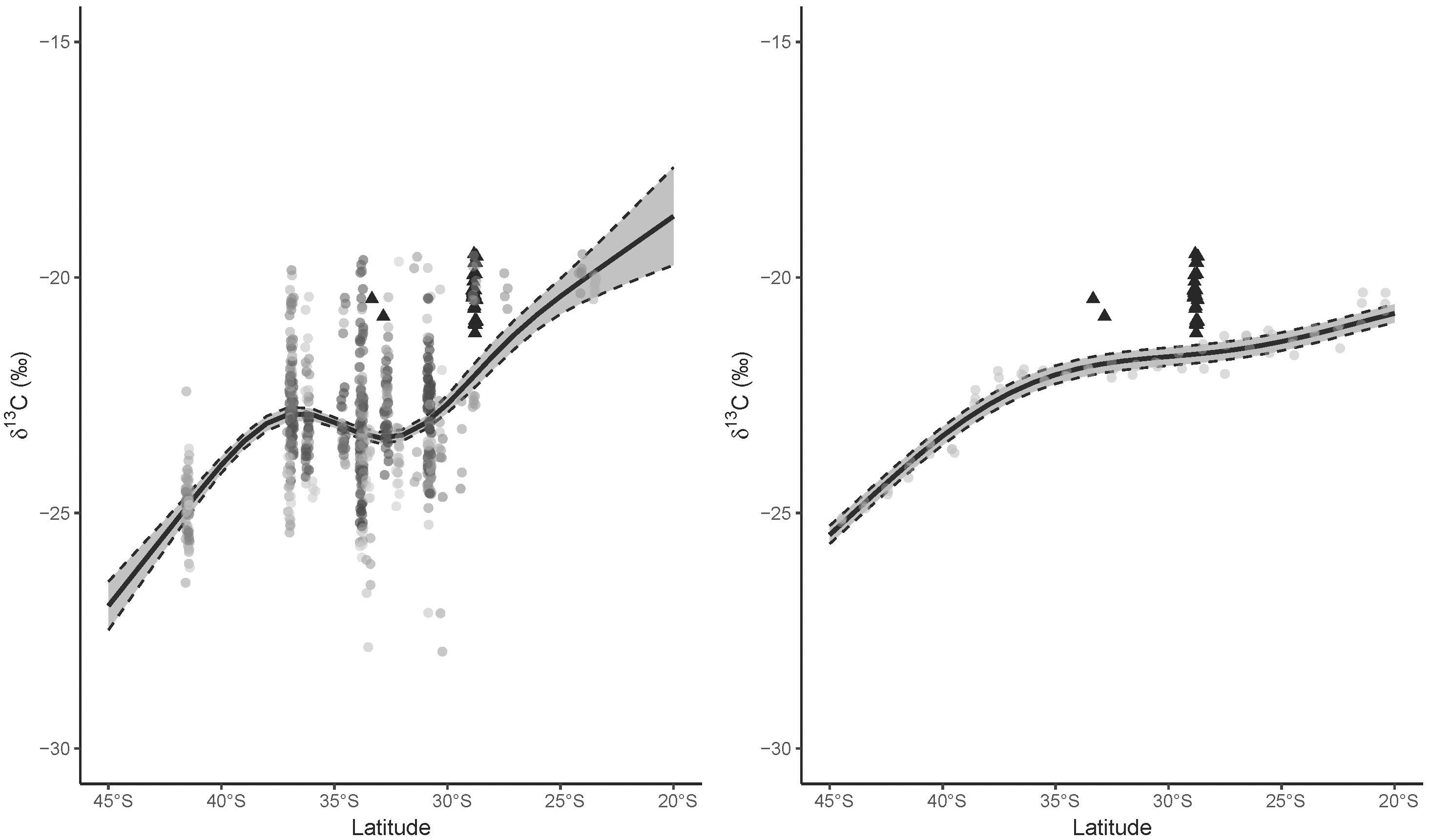
Figure 2. Relationship between latitude and δ13C values calculated from (left) trophic enrichment-adjusted values of fishes and cephalopods (only mean individual values displayed, species in colors) collected along the east coast of Australia (black dashed lines indicate 95% confidence interval around the model), and (right) the comparable range of yearly mean coastal δ13Cplk values from the NEMO-MEDUSA data. Different species used to calculate the relationship indicated in different colored circles, and great hammerhead shark (Sphyrna mokarran) mean individual trophic enrichment-adjusted values are indicated in black triangles along with their associated latitude at capture.
Predicted Habitat Range of Sphyrna mokarran
The likely latitude of foraging estimated for the modeled population for S. mokarran using field sampled δ13Cfish values as the reference had a normal distribution, with nearly 80% of the population situated between 26°S and 18°S, which was the northern-most extent of where sample-driven data were collected. The highest proportion of the population was near Gladstone, Queensland (Figure 3). In comparison, while the mechanistic model also suggests the S. mokarran geographic range was north of capture locations, the core geographic range was concentrated north of 15°S (Figure 3).
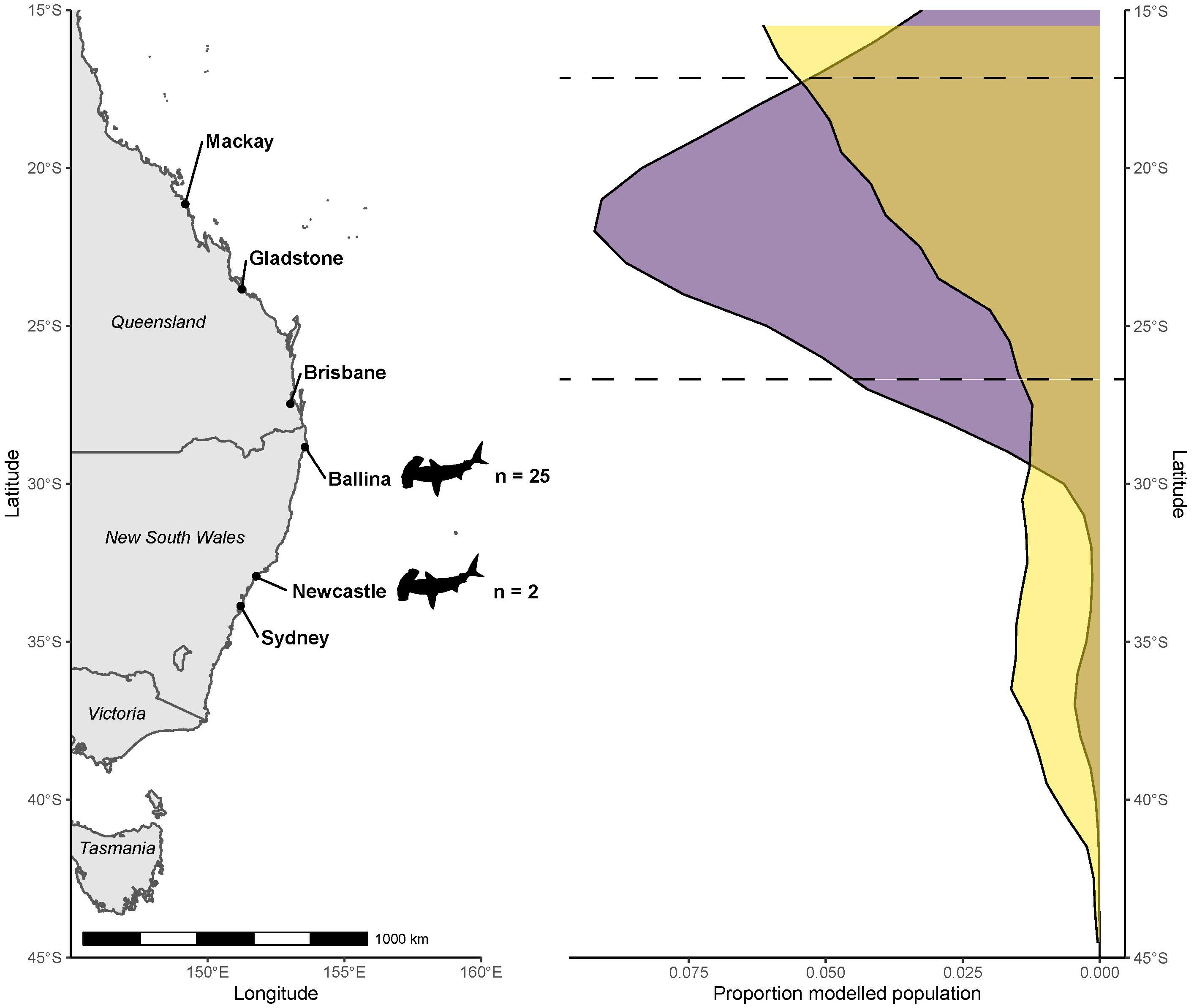
Figure 3. Modeled population geographic range of coastal great hammerhead sharks (Sphyrna mokarran) inferred from δ13C stable isotope values of their muscle tissues, and those from the various marine fish species, used to produce a latitude - δ13Cfish value relationship (purple). Corresponding modeled population density from the mechanistic NEMO-MEDUSA data shown for comparison (yellow). Dashed lines indicate latitudes that contained nearly 80% of the modeled population from the sample-driven model. Locations where great hammerhead shark samples were collected are indicated by shark outlines.
The likely latitude of foraging estimated for the modeled population for S. mokarran using mechanistically modeled δ13Cplk values as the reference was concentrated north of the NSW/Queensland border and probably extended further north than 10°S (Figure 4). The largest proportion of the population was measured along the coast of Queensland, and at 12°S, which broadly extended east and west at those latitudes and decreased north of this. It also extended east from 20°S with a relatively high proportion near the Des Belona plateau west of New Caledonia.
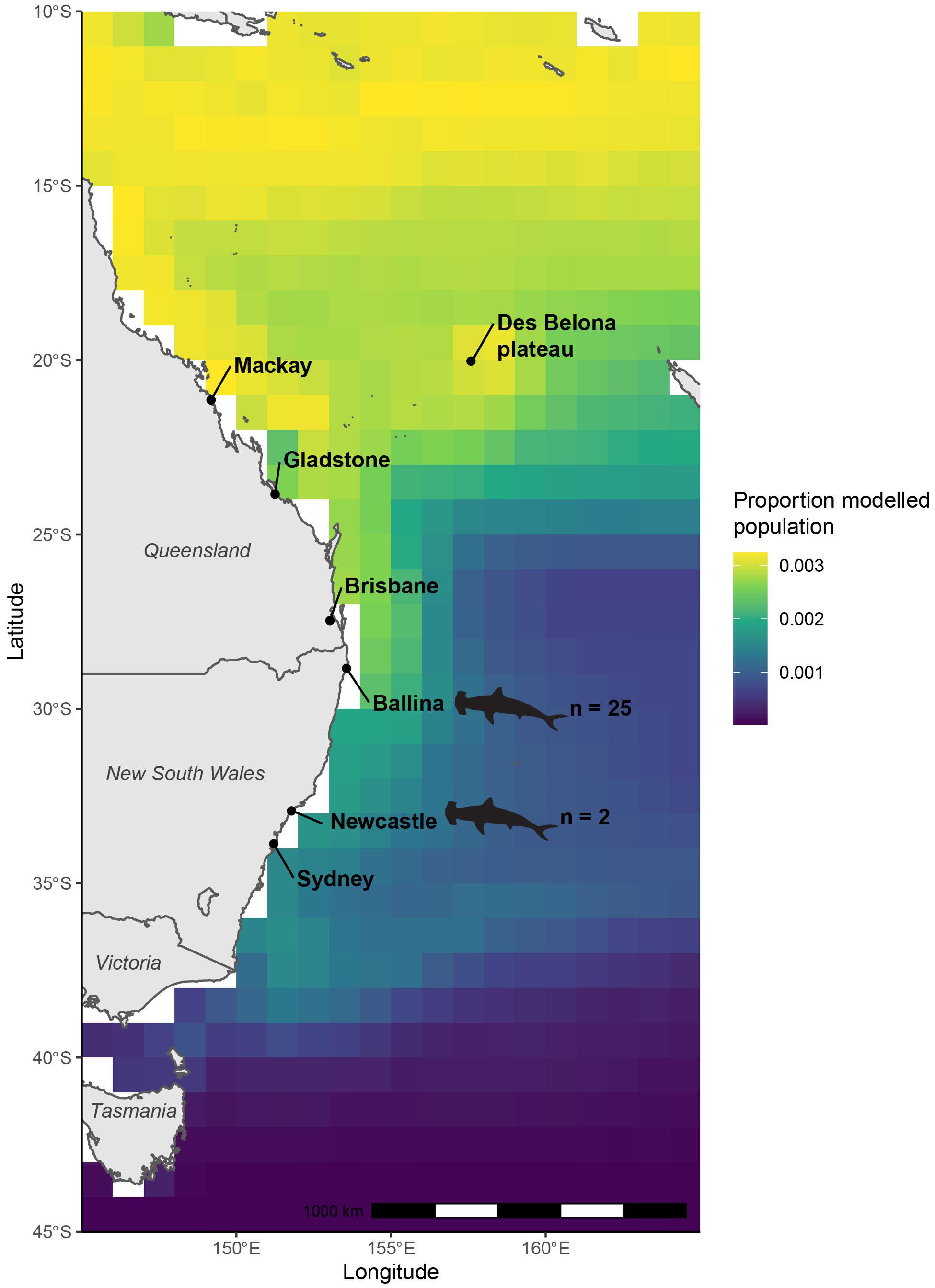
Figure 4. Modeled population geographic range of great hammerhead sharks (Sphyrna mokarran) inferred from δ13C stable isotope values of muscle tissues of great hammerhead sharks and biomass-weighted annual median δ13Cplk values of oceanic phytoplankton extracted from NEMO-MEDUSA framework. Locations where great hammerhead shark samples were collected are indicated by shark outlines.
Cross-Checking of Validity of Models
Previous work (Raoult et al., 2020) indicated that core Pristiophorus spp. habitat (where highest abundances and records are recorded) is on the north-east side of Bass Strait near the Victoria – New South Wales border (∼37°S) (Supplementary Figure 2). The field sampled model suggested a concentration around Bass Strait (40°S), providing the second peak more north than 30°S is ignored (Supplementary Figure 3). The NEMO-MEDUSA modeling agreed with the sample-based approach, with the highest proportion of modeled population at 40°S and decreasing rapidly north of 37°S (Supplementary Figure 4).
Discussion
Both the sampling-based and mechanistic (NEMO-MEDUSA) approaches used in this study support a hypothesis that the sampled S. mokarran caught in NSW bather-protection gillnets off in south-eastern Australia relied on food resources obtained further north off eastern Australia. And the species is likely only present in south-eastern Australian waters during the warmer summer/autumn months. If so, there may be no permanent resident population of S. mokarran in NSW waters, and any S. mokarran observed in this area are likely to be seasonal vagrants that fed primarily in Queensland waters.
Such wide latitudinal movements among S. mokarran support known migrations across other areas of the species distribution (especially in the Atlantic Ocean), and are similar to those recorded for regional carcharhinids such as the bull shark (Carcharhinus leucas) (Lee et al., 2019), and for the reef manta ray (M. alfredi) (Couturier et al., 2011). These movements may reflect physiologically driven preferences for sub-tropical and tropical water temperatures, which in the austral summer come with abundant inshore food sources such as schooling Australian cownose rays (Rhinoptera neglecta) (Tagliafico et al., 2020). This hypothesis aligns with the mechanistic model for Australian S. mokarran, which suggests a geographic range as far north as 10°S. Certainly the species is occasionally recorded in catches of baited drumlines off Cairns (17°S) (QLD shark control data, 20202).
While it is possible that some of the geographic range determined here could be at least be partially affected by prey species feeding at a higher latitude, the sporadic records of S. mokarran during the austral summer in NSW suggest the observed patterns are real. Targeted sampling of S. mokarran within the northern end of the geographic range near Cairns, QLD (identified as ‘core’ here) should help validate whether the inferences drawn are correct. Given the ongoing fisheries pressures on this species in this population’s eastern Australian core geographic range off Queensland (Roff et al., 2018), we suggest inter-state cooperation is necessary to address the above shortfalls and to collaboratively protect S. mokarran throughout its eastern Australian distribution.
Methodological Considerations
The outputs of the two methods produced different patterns, but both suggested that south-eastern Australia was not a core habitat for S. mokarran. The sample-driven approach implied a more constrained range, while the mechanistic approach suggested a range that started at a similar latitude, but extended further north, with peak density distributions of the populations that were ∼6° different. When applying the approaches to more southerly Pristiophorus spp., both aligned well with the known distributions of the species—provided open-ocean patterns that extend north and east of 30°S and 155°E, respectively, are ignored, since Pristiophorus spp. only occur in south-eastern Australia on the continental shelf or slope.
One possible common factor precluding the complete alignment of methods for both S. mokarran and Pristiophorus spp. was the low number of baseline samples at the extreme distributions of the models (north and south), which would increase sensitivity for error. In such cases, the outputs from the mechanistic model may be more reliable until broader datasets are obtained.
Notwithstanding the above, either the mechanistic or sample-driven approaches could be used to determine the broad geographic range of captured populations of both species. Using a single-axis (i.e., latitudinal), sample-driven approach that does not account for longitudinal variation was sufficiently informative and able to answer the research question with a coastline that aligns with latitudinal change in δ13C values, while costing considerably less to produce than an approach that would include longitudinal data.
Despite the utility of our approach, there are several assumptions that need to be considered when interpreting the results and extending to other species. In particular, 13C stable isotope ratios are primarily driven by diet rather than geographic location, with terrestrial, coastal, and neritic (macrophyte, phytoplankton, saltmarsh, and seagrass) sources all having distinct carbon values as a result of different photosynthetic pathways (Raoult et al., 2018) across a greater isotopic range (∼20‰) than other factors such as depth and latitude (McMahon et al., 2013). This means that for studies aiming to extract a geographic signal from stable isotope values, data will inherently have wide variability because of individual patterns in diet and space use, especially for species that occupy coastal areas. The variability of the sample-driven data for a single species at a single latitude are evidence of these effects. However, by incorporating large data sets as in the present study and others (Bird et al., 2018; Logan et al., 2020), it is possible to decipher the underlying geographic patterns at useful levels of spatial resolution, especially on a continental-scale latitudinal plane where the spatial variation of 13C stable isotope ratios is more easily detected.
Studies seeking to use this model in Australia or replicate the approach elsewhere should consider that species relying on estuarine or terrestrial productivity (like C. leucas) might not be appropriate focal subjects. For such species that rely on estuarine productivity, it is likely that localized primary producers will have a greater influence on δ13C values than phytoplankton-derived productivity and their latitudinal patterns. Where coastal species are the focus (as in this case), larger sampling populations for both the focal species and the sampling-based model should be obtained to ensure that coastal variability is adequately assessed. The similarity of the sample-driven model we produced from coastal species to those produced from pelagic sources obtained previously in the same area (Revill et al., 2009) provides evidence that latitudinal coastal stable isotope patterns are not dissimilar from pelagic ones, and that latitudinal variation can be measured from coastal species on sufficiently large scales. We also draw on results of Bird et al. (2018) who showed (using a global compilation of δ13C data from sharks tissues) that the δ13C values of muscle tissues in coastal and neritic sharks do indeed follow latitudinal gradients predicted and measured in phytoplankton, implying that overall, phytoplankton provide the majority of carbon fueling food webs leading to coastal shark production. Thus, while coastal productivity likely influences δ13C values of study species as well as species used for sample-driven models, it should still be possible to infer data from phytoplankton-based models if researchers are aware of these possible influences.
The eastern coastline of Australia is a challenging geographic area in which to apply this approach because the poleward-flowing East Australian Current strongly impacts annual patterns in δ13C values. Consequently, the presence of detectable patterns implies that our approach should be even more successful in other parts of the world with less dynamic circulation. More specifically, the patterns for both our mechanistic and sample-driven approaches were similar to previous attempts at sample-driven approaches obtained from a broad suite of consumers collected further offshore (Revill et al., 2009), indicating that such an approach would be repeatable and reusable on decadal scales. Similarly, the use of diet-tissue discrimination factors to correct for isotopic enrichment with trophic level has uncertainty, which we addressed using MCMC simulations. Due to the low relative difference between low and high latitude δ13C values (7‰ across 25° of latitude or approximately 2700 km), we also reiterate that this approach cannot be used to infer fine-scale (<1° of latitude) geographic location. Rather, as in this study, interpretations are limited to answering questions on broad geographic ranges such as the direction (north, south, east, west) of the habitat relative to capture point.
Multimodality of modeled geographic ranges can occur as indicated here, implying the possibility of more than one geographic habitat for one sample population. Multimodality could be driven by individual preferences in diet, which has been identified in S. mokarran and other elasmobranchs (Matich et al., 2011; Raoult et al., 2019)—although larger sampling sizes should reduce the likelihood of multimodality with this approach. We suggest assuming core habitat ranges should be connected to the nearest identified core habitat, and to discount other detected habitats as possible artifacts. If biological information is available for the species (i.e., limits of thermal tolerances or bathymetry links) these data can be used to refine the modeled outputs. For example, in our case it is unlikely that some of the population extends southeast into the Pacific Ocean as the model suggests since those water temperatures are likely outside of physical tolerances for this species, although S. lewini has been known to dive periodically to waters at ∼5°C (Jorgensen et al., 2009). For species for which there is little biological information available, outputs may be less reliable if multimodal distributions are apparent. If researchers using this approach are aware of such limitations, then this method is robust for determining core geographic range on a broad scale for many wide-ranging marine organisms.
Beyond methodological considerations, projects attempting to use similar approaches to examine the geographic patterns of other species should be aware of some of the broader issues we encountered. For example, extrapolating geographic ranges for species that may occur beyond the sample-driven latitudinal range (further north of 20°S in our case) can lead to greater uncertainty. In those instances, we recommend researchers compare their sample-driven patterns to those from the NEMO-MEDUSA data or source samples from latitudinal extremes in the published literature. The model presented here does not account for known habitat preference (like bathymetry) that would otherwise be constraining, and the results should be interpreted accordingly. Ideally, those replicating the approach would incorporate known habitat ranges into the model to constrain results more appropriately. We highlight that the strength of our approach is the ability to use bulk muscle stable isotope values to populate the sampling-based relationship from various species of sources, provided individual sample %C and %N (to correct for lipids) data are available. In our instance there were very few usable data from north of Gladstone, Queensland, which led to a steep extrapolation of δ13C values that might not be valid. Other studies conducted in areas that have been more broadly sampled historically (i.e., the north Atlantic) may be able to rely on previous work more readily (Le Loc’h et al., 2008).
Appropriate thought needs to be given to the temporal scale being studied, as marine productivity varies seasonally, interannually, and gradually with climate (Gonzalez-Rodriguez, 1994; San Martin et al., 2006; Shen et al., 2015). The use of higher trophic level animals should result in long temporal averaging of signals through food chains associated with addition of turnover rates. Any seasonal variability in carbon source δ13C values will thus be strongly attenuated through food chains and in animals with slow isotopic assimilation rates. Tissue selection for both target species and sample-driven isoscape creation will also relate directly to the interpretations that can be extracted from this approach. The isoscape designed here used muscle primarily because it has approximately annual turnover rates, depending on the age class of the sampled animals (Kim et al., 2012). Since the objective here was to determine long-term geographic range, tissues with longer turnover like muscle or cartilage (Malpica-Cruz et al., 2012) were preferable. Turnover rates of the mechanistic and sampling-based isoscapes also need to be examined across similar temporal scales as the target population. In our case, we examined annual means in the mechanistic model to align with muscle tissue selection. If researchers wanted to study short-term patterns, they could sample tissues that turn over rapidly like blood or liver, and adjust mechanistic models accordingly. However, we recommend longer turnover tissues like muscle may provide more robust results that will average localized changes in productivity that would otherwise affect results.
Appropriate consumer tissue preparation prior to these approaches is critical. Urea and lipids affect δ15N and δ13C values (Carlisle et al., 2016), and these patterns are difficult to accurately correct for using mathematical approaches (Shipley et al., 2017). Incorporating uncertainty (e.g., with MCMC approach) in diet-tissue discrimination factors that account for lipid and urea effects helps alleviate this issue, but results would still be centered based on the mean of these values, which may not be appropriate for the study species. We strongly suggest that lipid and urea extractions are conducted on all bulk tissues used for geographic range calculations to reduce the uncertainty that can result from these effects.
When selecting species to target for sampling-based reference isoscape creation, we initially assumed that juvenile zooplanktivorous fishes (e.g., Abudefduf spp.) would provide a more reliable signal than fishes at higher trophic levels. However, after examining the stable isotope values from multiple local studies it was apparent that some of the northernmost values from the southern Great Barrier Reef were likely feeding on turf algae rather than plankton, and these data were excluded from the analyses. We therefore recommend comparing corrected δ13Cfish values to geographically similar turf algae and plankton values where possible to help inform the sampling-based data in this way. Signal noise in juvenile planktivorous fishes could also be caused by rapid (<20 days) tissue turnover (Weidel et al., 2011), which could reflect seasonal stable isotope values rather than the yearly values recorded in larger, slower growing fishes. Of note, even tertiary predators like flathead Platycephalus spp. and pink snapper Pagrus auratus provided useful reference information, which suggests that targeted species can be from broad trophic ranges, provided these species have relatively constrained geographic ranges. Validating the outputs from this approach would, however, strengthen its reliability for management, and this could be done by consistently sampling species with known restricted habitat ranges along the coast.
Notwithstanding the stated caveats, clearly mechanistic isoscape models such as the NEMO-MEDUSA isotope extension (Magozzi et al., 2017) can be used to infer spatial influences on isotopic variation in measured samples and therefore geographic distributions (e.g., Bird et al., 2018; Trueman et al., 2019). To use this approach, calibration is crucial between the mechanistic isoscape and the study samples. This calibration must consider isotopic effects associated with trophic enrichment, tissue composition, and time averaging. Accounting for these issues is not trivial, and we recommend that mechanistic models are not used in isolation to infer geographic assignments. Rather, the isotopic composition of geo-referenced field samples (using the broad reference species approach outlined here) should be used to first determine appropriate calibrations. Such an approach would still be comparatively low-cost relative to large tagging programs, especially since the data can be re-used for different species.
Data Availability Statement
The original contributions presented in the study are included in the article/Supplementary Material, further inquiries can be directed to the corresponding author/s.
Ethics Statement
The animal study was reviewed and approved by the New South Wales Animal Care and Ethics Committee (NSW ACEC ref no. 06/08).
Author Contributions
VR, CT, VP, MB, JW, and TG conceived the study. VR conducted the fieldwork and sample analysis. KK, BG, DB, IN, and LC provided the additional data and advice on analyses. VR and CT analyzed the results and wrote the initial draft. VR, CT, VP, MB, JW, TG, KK, BG, DB, IN, and LC wrote the follow up draft, provided feedback for additional analyses, and general improvements. All the authors contributed to the article and approved the submitted version.
Funding
This research was part-funded through a grant from the Sea World Research and Rescue Foundation (SWRRFI) to VR, VP, TG, and JW, and from the NSW Department of Primary Industries. The sampling and stable isotope analysis of the zooplanktivorous fish samples was supported by an Australian Research Council Discovery grant (DP170101722) to IN, DB, and BG. Manta ray sampling and isotopic analyses were funded by the Australian Research Council Linkage Grant (LP110100712), Earthwatch Institute Australia, Sea World Research and Rescue Foundation Inc., Lady Elliot Island Eco Resort and Manta Lodge and Scuba Centre in Australia.
Conflict of Interest
The authors declare that data from a previous study used here was funded partly by Sibelco Pty Ltd. This funder was not involved in the study design, collection, analysis, interpretation of data, the writing of this article or the decision to submit for publication. The authors declare that the research was conducted in the absence of any commercial or financial relationships that could be construed as a potential conflict of interest.
Acknowledgments
We thank the skippers and crews of the various NSW bather-protection gillnet contractors for their assistance at sea, and NSW DPI Fisheries staff for logistic support. Many thanks to Chris Brown who provided feedback on the approach. Thanks to Louise Tosetto for her assistance during sampling.
Supplementary Material
The Supplementary Material for this article can be found online at: https://www.frontiersin.org/articles/10.3389/fmars.2020.594636/full#supplementary-material
Footnotes
- ^ www.retsch.com
- ^ https://www.daf.qld.gov.au/__data/assets/excel_doc/0013/300064/shark-catch-stats-2001-to-dec2016.xls
References
Barnes, T. C., Rogers, P. J., Wolf, Y., Madonna, A., Holman, D., Ferguson, G. J., et al. (2019). Dispersal of an exploited demersal fish species (Argyrosomus japonicus, Sciaenidae) inferred from satellite telemetry. Mar. Biol. 166:125.
Bird, C. S., Veríssimo, A., Magozzi, S., Abrantes, K. G., Aguilar, A., Al-Reasi, H., et al. (2018). A global perspective on the trophic geography of sharks. Nat. Ecol. Evol. 2, 299–305.
Block, B. A. (2019). “Use of electronic tags to reveal migrations of atlantic Bluefin Tunas,” in The Future of Bluefin Tunas: Ecology, Fisheries Management, and Conservation, ed. B. A. Block (JHU Press), 94.
Bond, A. L., and Diamond, A. W. (2011). Recent Bayesian stable-isotope mixing models are highly sensitive to variation in discrimination factors. Ecol. Appl. 21, 1017–1023. doi: 10.1890/09-2409.1
Broadhurst, M. K., and Cullis, B. R. (2020). Mitigating the discard mortality of non-target, threatened elasmobranchs in bather-protection gillnets. Fish. Res. 222:105435. doi: 10.1016/j.fishres.2019.105435
Carlisle, A. B., Litvin, S. Y., Madigan, D. J., Lyons, K., Bigman, J. S., Ibarra, M., et al. (2016). Interactive effects of urea and lipid content confound stable isotope analysis in elasmobranch fishes. Can. J. Fish. Aquat. Sci. 74, 419–428. doi: 10.1139/cjfas-2015-0584
Caut, S., Angulo, E., and Courchamp, F. (2009). Variation in discrimination factors (Δ15N and Δ13C): the effect of diet isotopic values and applications for diet reconstruction. J. Appl. Ecol. 46, 443–453. doi: 10.1111/j.1365-2664.2009.01620.x
Cooter, E. J., and Schwede, D. B. (2000). Sensitivity of the national oceanic and atmospheric administration multilayer model to instrument error and parameterization uncertainty. J. Geophys. Res. Atmos. 105, 6695–6707. doi: 10.1029/1999jd901080
Couturier, L. I., Jaine, F. R., Townsend, K. A., Weeks, S. J., Richardson, A. J., and Bennett, M. B. (2011). Distribution, site affinity and regional movements of the manta ray, Manta alfredi (Krefft, 1868), along the east coast of Australia. Mar. Freshw. Res. 62, 628–637. doi: 10.1071/mf10148
Couturier, L. I., Rohner, C. A., Richardson, A. J., Marshall, A. D., Jaine, F. R., Bennett, M. B., et al. (2013). Stable isotope and signature fatty acid analyses suggest reef manta rays feed on demersal zooplankton. PLoS One 8:e77152. doi: 10.1371/journal.pone.0077152
Eurich, J., Matley, J., Baker, R., Mccormick, M., and Jones, G. (2019). Stable isotope analysis reveals trophic diversity and partitioning in territorial damselfishes on a low-latitude coral reef. Mar. Biol. 166:17.
Frédérich, B., Fabri, G., Lepoint, G., Vandewalle, P., and Parmentier, E. (2009). Trophic niches of thirteen damselfishes (Pomacentridae) at the Grand Récif of Toliara, Madagascar. Ichthyol. Res. 56, 10–17. doi: 10.1007/s10228-008-0053-2
Fry, B., Scalan, R., and Parker, P. (1983). 13C/12C ratios in marine food webs of the Torres Strait, Queensland. Mar. Freshw. Res. 34, 707–715. doi: 10.1071/mf9830707
Gonzalez-Rodriguez, E. (1994). Yearly variation in primary productivity of marine phytoplankton from Cabo Frio (RJ, Brazil) region. Hydrobiologia 294, 145–156. doi: 10.1007/bf00016855
Greenwood, N., Sweeting, C., and Polunin, N. (2010). Elucidating the trophodynamics of four coral reef fishes of the Solomon Islands using δ 15 N and δ 13 C. Coral Reefs 29, 785–792. doi: 10.1007/s00338-010-0626-1
Guttridge, T., Van Zinnicq Bergmann, M., Bolte, C., Howey, L., Finger, J., Kessel, S., et al. (2017). Philopatry and regional connectivity of the great hammerhead shark, Sphyrna mokarran in the US and Bahamas. Front. Mar. Sci. 4:3. doi: 10.3389/fmars.2017.00003
Hill, J., Mcquaid, C., and Kaehler, S. (2006). Biogeographic and nearshore-offshore trends in isotope ratios of intertidal mussels and their food sources around the coast of southern Africa. Mar. Ecol. Prog. Ser. 318, 63–73. doi: 10.3354/meps318063
Hobday, A. J., Hartog, J. R., Spillman, C. M., and Alves, O. (2011). Seasonal forecasting of tuna habitat for dynamic spatial management. Can. J. Fish. Aquat. Sci. 68, 898–911. doi: 10.1139/f2011-031
Hobson, K. A., and Cherel, Y. (2006). Isotopic reconstruction of marine food webs using cephalopod beaks: new insight from captively raised Sepia officinalis. Can. J. Zool. 84, 766–770. doi: 10.1139/z06-049
Hofman, M., Hayward, M., Heim, M., Marchand, P., Rolandsen, C. M., Mattisson, J., et al. (2019). Right on track? Performance of satellite telemetry in terrestrial wildlife research. PLoS One 14:e0216223. doi: 10.1371/journal.pone.0216223
Holmes, B. J., Pepperell, J. G., Griffiths, S. P., Jaine, F. R., Tibbetts, I. R., and Bennett, M. B. (2014). Tiger shark (Galeocerdo cuvier) movement patterns and habitat use determined by satellite tagging in eastern Australian waters. Mar. Biol. 161, 2645–2658. doi: 10.1007/s00227-014-2536-1
Hussey, N. E., Brush, J., Mccarthy, I. D., and Fisk, A. T. (2010). δ 15 N and δ 13 C diet-tissue discrimination factors for large sharks under semi-controlled conditions. Compar. Biochem. Physiol. Part A Mol. Integrat. Physiol. 155, 445–453. doi: 10.1016/j.cbpa.2009.09.023
Jorgensen, S., Klimley, A., and Muhlia-Melo, A. (2009). Scalloped hammerhead shark Sphyrna lewini, utilizes deep-water, hypoxic zone in the Gulf of California. J. Fish Biol. 74, 1682–1687. doi: 10.1111/j.1095-8649.2009.02230.x
Kim, S. L., Del Rio, C. M., Casper, D., and Koch, P. L. (2012). Isotopic incorporation rates for shark tissues from a long-term captive feeding study. J. Exper. Biol. 215, 2495–2500. doi: 10.1242/jeb.070656
Kingsbury, K. M., Gillanders, B. M., Booth, D. J., Coni, E. O., and Nagelkerken, I. (2020). Range-extending coral reef fishes trade-off growth for maintenance of body condition in cooler waters. Sci. Total Environ. 703:134598. doi: 10.1016/j.scitotenv.2019.134598
Kopp, D., Lefebvre, S., Cachera, M., Villanueva, M. C., and Ernande, B. (2015). Reorganization of a marine trophic network along an inshore-offshore gradient due to stronger pelagic-benthic coupling in coastal areas. Prog. Oceanogr. 130, 157–171. doi: 10.1016/j.pocean.2014.11.001
Le Loc’h, F., Hily, C., and Grall, J. (2008). Benthic community and food web structure on the continental shelf of the Bay of Biscay (North Eastern Atlantic) revealed by stable isotopes analysis. J. Mar. Syst. 72, 17–34. doi: 10.1016/j.jmarsys.2007.05.011
Lee, K., Smoothey, A., Harcourt, R., Roughan, M., Butcher, P., and Peddemors, V. (2019). Environmental drivers of abundance and residency of a large migratory shark, Carcharhinus leucas, inshore of a dynamic western boundary current. Mar. Ecol. Prog. Ser. 622, 121–137. doi: 10.3354/meps13052
Logan, J., Pethybridge, H., Lorrain, A., Somes, C., Allain, V., Bodin, N., et al. (2020). Global patterns and inferences of tuna movements and trophodynamics. Deep Sea Res. Part II Top. Stud. Oceanogr. 175:104775. doi: 10.1016/j.dsr2.2020.104775
Madigan, D. J., Chiang, W.-C., Wallsgrove, N. J., Popp, B. N., Kitagawa, T., Choy, C. A., et al. (2016). Intrinsic tracers reveal recent foraging ecology of giant Pacific bluefin tuna at their primary spawning grounds. Mar. Ecol. Prog. Ser. 553, 253–266. doi: 10.3354/meps11782
Magozzi, S., Yool, A., Vander Zanden, H., Wunder, M., and Trueman, C. (2017). Using ocean models to predict spatial and temporal variation in marine carbon isotopes. Ecosphere 8:e01763. doi: 10.1002/ecs2.1763
Malpica-Cruz, L., Herzka, S. Z., Sosa-Nishizaki, O., and Escobedo-Olvera, M. A. (2013). Tissue-specific stable isotope ratios of shortfin mako (Isurus oxyrinchus) and white (Carcharodon carcharias) sharks as indicators of size-based differences in foraging habitat and trophic level. Fish. Oceanogr. 22, 429–445. doi: 10.1111/fog.12034
Malpica-Cruz, L., Herzka, S. Z., Sosa-Nishizaki, O., and Lazo, J. P. (2012). Tissue-specific isotope trophic discrimination factors and turnover rates in a marine elasmobranch: empirical and modeling results. Can. J. Fish. Aquat. Sci. 69, 551–564. doi: 10.1139/f2011-172
Matich, P., Heithaus, M. R., and Layman, C. A. (2011). Contrasting patterns of individual specialization and trophic coupling in two marine apex predators. J. Anim. Ecol. 80, 294–305. doi: 10.1111/j.1365-2656.2010.01753.x
McMahon, K. W., Hamady, L. L., and Thorrold, S. R. (2013). A review of ecogeochemistry approaches to estimating movements of marine animals. Limnol. Oceanogr. 58, 697–714. doi: 10.4319/lo.2013.58.2.0697
Olin, J. A., Hussey, N. E., Grgicak-Mannion, A., Fritts, M. W., Wintner, S. P., and Fisk, A. T. (2013). Variable δ15N diet-tissue discrimination factors among sharks: implications for trophic position, diet and food web models. PLoS One 8:e77567. doi: 10.1371/journal.pone.0077567
Post, D. M. (2002). Using stable isotopes to estimate trophic position: models, methods, and assumptions. Ecology 83, 703–718. doi: 10.1890/0012-9658(2002)083[0703:usitet]2.0.co;2
Post, D. M., Layman, C. A., Arrington, D. A., Takimoto, G., Quattrochi, J., and Montaña, C. G. (2007). Getting to the fat of the matter: models, methods and assumptions for dealing with lipids in stable isotope analyses. Oecologia 152, 179–189. doi: 10.1007/s00442-006-0630-x
Queiroz, N., Humphries, N. E., Couto, A., Vedor, M., Da Costa, I., Sequeira, A. M., et al. (2019). Global spatial risk assessment of sharks under the footprint of fisheries. Nature 572, 461–466.
Raoult, V., Broadhurst, M. K., Peddemors, M., Williamson, M., and Gaston, M. (2019). Resource use of great hammerhead sharks Sphyrna mokarran off eastern Australia. J. Fish Biol. 95, 1430–1440. doi: 10.1111/jfb.14160
Raoult, V., Gaston, T. F., and Taylor, M. D. (2018). Habitat-fishery linkages in two major south-eastern Australian estuaries show that the C4 saltmarsh plant Sporobolus virginicus is a significant contributor to fisheries productivity. Hydrobiologia 811, 221–238. doi: 10.1007/s10750-017-3490-y
Raoult, V., Gaston, T. F., and Williamson, J. E. (2015). Not all sawsharks are equal: species of co-existing sawsharks show plasticity in trophic consumption both within and between species. Can. J. Fish. Aquat. Sci. 72, 1769–1775. doi: 10.1139/cjfas-2015-0307
Raoult, V., Peddemors, V., Rowling, K., and Williamson, J. E. (2020). Spatiotemporal distributions of two sympatric sawsharks (Pristiophorus cirratus and P. nudipinnis) in south-eastern Australian waters. Mar. Freshw. Res. 71, 1342–1354. doi: 10.1071/MF19277
Rau, G., Sweeney, R., and Kaplan, I. (1982). Plankton 13C: 12C ratio changes with latitude: differences between northern and southern oceans. Deep Sea Res. Part A Oceanogr. Res. Pap. 29, 1035–1039. doi: 10.1016/0198-0149(82)90026-7
Revill, A. T., Young, J. W., and Lansdell, M. (2009). Stable isotopic evidence for trophic groupings and bio-regionalization of predators and their prey in oceanic waters off eastern Australia. Mar. Biol. 156, 1241–1253. doi: 10.1007/s00227-009-1166-5
Rigby, C., Dulvy, N., Barreto, R., Carlson, J., Fernando, D., Fordham, S., et al. (2019). Sphyrna mokarran. IUCN Red List Threat. Spec. 2019:e.T39385A2918526.
Roff, G., Brown, C. J., Priest, M. A., and Mumby, P. J. (2018). Decline of coastal apex shark populations over the past half century. Commun. Biol. 1:223.
San Martin, E., Irigoien, X., Roger, P. H., Urrutia, ÂL., Zubkov, M. V., and Heywood, J. L. (2006). Variation in the transfer of energy in marine plankton along a productivity gradient in the Atlantic Ocean. Limnol. Oceanogr. 51, 2084–2091. doi: 10.4319/lo.2006.51.5.2084
Sequeira, A., Heupel, M., Lea, M. A., Eguíluz, V. M., Duarte, C. M., Meekan, M., et al. (2019). The importance of sample size in marine megafauna tagging studies. Ecol. Appl. 29:e01947.
Shen, J., Schoepfer, S. D., Feng, Q., Zhou, L., Yu, J., Song, H., et al. (2015). Marine productivity changes during the end-Permian crisis and Early Triassic recovery. Earth Sci. Rev. 149, 136–162. doi: 10.1016/j.earscirev.2014.11.002
Shipley, O. N., Olin, J. A., Polunin, N. V., Sweeting, C. J., Newman, S. P., Brooks, E. J., et al. (2017). Polar compounds preclude mathematical lipid correction of carbon stable isotopes in deep-water sharks. J. Exper. Mar. Biol. Ecol. 494, 69–74. doi: 10.1016/j.jembe.2017.05.002
Somes, C. J., Schmittner, A., Galbraith, E. D., Lehmann, M. F., Altabet, M. A., Montoya, J. P., et al. (2010). Simulating the global distribution of nitrogen isotopes in the ocean. Glob. Biogeochem. Cycles 24:GB4019. doi: 10.1029/2009GB003767
St. John Glew, K., Graham, L. J., Mcgill, R. A., and Trueman, C. N. (2019). Spatial models of carbon, nitrogen and sulphur stable isotope distributions (isoscapes) across a shelf sea: an INLA approach. Methods Ecol. Evol. 10, 518–531. doi: 10.1111/2041-210x.13138
Sumpton, W., Taylor, S., Gribble, N., Mcpherson, G., and Ham, T. (2011). Gear selectivity of large-mesh nets and drumlines used to catch sharks in the Queensland Shark Control Program. Afr. J. Mar. Sci. 33, 37–43. doi: 10.2989/1814232x.2011.572335
Tagliafico, A., Butcher, P. A., Colefax, A. P., Clark, G. F., and Kelaher, B. P. (2020). Variation in cownose ray Rhinoptera neglecta abundance and group size on the central east coast of Australia. J. Fish Biol. 96, 427–433. doi: 10.1111/jfb.14219
Trueman, C. N., Jackson, A. L., Chadwick, K. S., Coombs, E. J., Feyrer, L. J., Magozzi, S., et al. (2019). Combining simulation modeling and stable isotope analyses to reconstruct the last known movements of one of Nature’s giants. PeerJ 7:e7912. doi: 10.7717/peerj.7912
Weidel, B. C., Carpenter, S. R., Kitchell, J. F., and Vander Zanden, M. J. (2011). Rates and components of carbon turnover in fish muscle: insights from bioenergetics models and a whole-lake 13C addition. Can. J. Fish. Aquat. Sci. 68, 387–399. doi: 10.1139/f10-158
West, J. B., Bowen, G. J., Dawson, T. E., and Tu, K. P. (2009). Isoscapes: Understanding Movement, Pattern, and Process on Earth Through Isotope Mapping. Berlin: Springer.
Keywords: habitat range population distributions, movement, species distribution model, sharks, manta rays, stable isotopes, tracking, isoscape
Citation: Raoult V, Trueman CN, Kingsbury KM, Gillanders BM, Broadhurst MK, Williamson JE, Nagelkerken I, Booth DJ, Peddemors V, Couturier LIE and Gaston TF (2020) Predicting Geographic Ranges of Marine Animal Populations Using Stable Isotopes: A Case Study of Great Hammerhead Sharks in Eastern Australia. Front. Mar. Sci. 7:594636. doi: 10.3389/fmars.2020.594636
Received: 13 August 2020; Accepted: 12 November 2020;
Published: 03 December 2020.
Edited by:
Alastair Martin Mitri Baylis, South Atlantic Environmental Research Institute, Falkland IslandsReviewed by:
Aaron Carlisle, University of Delaware, United StatesLuciana C. Ferreira, Australian Institute of Marine Science (AIMS), Australia
Daniel James Madigan, University of Windsor, Canada
Copyright © 2020 Raoult, Trueman, Kingsbury, Gillanders, Broadhurst, Williamson, Nagelkerken, Booth, Peddemors, Couturier and Gaston. This is an open-access article distributed under the terms of the Creative Commons Attribution License (CC BY). The use, distribution or reproduction in other forums is permitted, provided the original author(s) and the copyright owner(s) are credited and that the original publication in this journal is cited, in accordance with accepted academic practice. No use, distribution or reproduction is permitted which does not comply with these terms.
*Correspondence: Vincent Raoult, VmluY2VudC5yYW91bHRAbmV3Y2FzdGxlLmVkdS5hdQ==