 Pietro D. Tomaselli
 Martin Dixen
- Ports and Offshore Technology, DHI, Copenhagen, Denmark
Safe and cost-efficient planning Operation&Maintenance (O&M) activities for the turbines of Offshore Wind Farms is crucial for the offshore wind industry. The execution of the planned tasks depends on the workability at sea. Workability assessments aim to find time periods, called weather windows, during which the personnel can execute the job at hand safely. Traditionally, weather windows analyses are based on thresholds applied on relevant metocean conditions in the area of interest, commonly wave height, wave period and wind speed. In this way, tasks are planned in windows during which the forecast metocean conditions do not exceed the defined thresholds. This paper presents a numerical tool that provides weather windows based on more direct measures of workability, that is seasickness on board during the trip to the turbines and bow motions, which endanger crew transfers from vessel to turbine. When assessing weather windows, such parameters better describe the actual decision drivers in a real operational setting than mere metocean thresholds, which are, in practical cases, discretionally judged by the O&M operator upon experience. Therefore, the reliability of workability predictions can increase, leading to financial gains for the wind industry and safer environment for O&M operators. The paper shows an application of the tool, where a full O&M scenario is simulated. The scenario comprises the transit from the port to the offshore site, the work carried out on the turbine and the transit back to the port. In particular, the application highlights the key capability of the tool of calculating vessel motions, which are elaborated to produce weather windows. With its low computational time-demand, the tool aims to support the decision-making processes that produce short- and long-term O&M plans.
1. Introduction
In the offshore wind industry, the Operation&Maintenance (O&M) activities are of utmost importance for a life long sustained power production from Offshore Wind Farms (OWFs). A failure of an element of the farm can cause a reduction or even a shutdown in the power production, which will lead to significant economic losses. It is important to adopt preventive maintenance strategies that can reduce the number of failures, through a planned series of O&M activities, such as inspections, reparations, and replacements.
Operation&Maintenance plans for OWFs are designed for both long- and short-term scenarios. A long-term plan, generally elaborated during the design phase, is the one in which the interventions are scheduled over 1 or more years. A short-term plan is for operational situations in which an already planned task is to be executed in the following few days or an unexpected failure happens and reparation needs to take place in the shortest possible time. In order to restrain the O&M related costs, which generally account for 25–30% of the total lifetime cost of an OWF (Marsh, 2007), it is necessary to maximize the effectiveness and efficiency of the O&M plans.
With the growth of the offshore wind industry, researchers have developed several numerical models that provide optimized scheduling of O&M tasks. A comprehensive review of the state-of-the-art models can be found in Seyr and Muskulus (2019), where the authors discussed the influential factors of the planning problem (weather conditions, logistics of personnel, vessels and spare parts, frequency of failures, cost valuations, maintenance strategy) and the different approaches to the solution (modeling techniques, optimization methods).
The present study focused on how weather conditions are taken into account as an influential factor of O&M planning. In fact, an O&M plan relies crucially on the assessment of weather windows, which are time periods where the metocean conditions (wave height, wave period, current speed, wind speed, among others) allow the O&M operator to execute the job. A weather window assessment usually consists of a simplified analysis of metocean data of the area of interest with thresholds chosen for a specific task. In particular, a weather window is a period during which the metocean conditions do not exceed the fixed thresholds for a time long enough to accomplish the execution of that task. The choice of the thresholds in a weather window assessment is driven primarily by health, safety, environmental demands and considerations for the O&M operator, along with economic factors for the wind industry operator. The metocean conditions that are considered suitable for a specific task must be such that the O&M operator can safely perform the task. But those thresholds should also guarantee that a sufficient number of workable hours is available, so that all the planned O&M activities can be executed, reducing the risk of downtime in the power production. Long term planning of chartering vessels that can handle rougher conditions and re-designing operations is also an important part of the optimization.
Increasing the reliability and suitability of weather window analyses leads to more efficient and effective O&M plans, which means lower O&M associated costs for the offshore wind industry and safer working conditions for the O&M operators. This holds especially in the short-term operational situations, where the decision-making process on the execution of the tasks becomes more critical. In practical cases, the risk is that a task is scheduled on a certain day, but though when the crew and the technicians meet in the morning at the port, they realize that sailing out is impracticable due to bad weather. It can also happen that they sail out and reach the OWF, but they realize that the task cannot be executed safely due to metocean conditions or the personnel becomes seasick during the trip out to OWF. In all these circumstances, the result is that the planned task is not executed and could have maybe been performed on another day that was wrongly assessed as not suitable for the scope. This ultimately leads to more failures and hence more days with individual turbines not producing electricity.
The availability of solid metocean data is an important and necessary condition to produce trustworthy weather window analyses for both long- and short-term scenarios. Combining modeling, satellite, and in-situ data as well as vessel mounted sensors provides an effective path to both improved deterministic and probabilistic forecasts (Sanchez-Arcilla et al., 2020), but this is only half the solution. Uncertainties also lie on the choice of the threshold parameters and values that determine the workability of a set of metocean conditions. In fact, thresholds like maximum acceptable significant wave height and peak wave period are not direct measures of the actual feasibility of a task, but indirect parameters. As an example, if an O&M task involves the use of a crane to lift a heavy cargo of spare parts to a turbine, thresholds are applied to maximum acceptable wave height, wave period, and wind speed that would not cause dangerous motions of the cargo, hence the thresholds are not directly applied on to the motions of the cargo, which cause the actual risk. In many practical cases, the thresholds on metocean conditions are not estimated anyhow, but rather the decision to start an operation is based on the experience of the O&M operator.
This paper presents the development and the application of a numerical tool that assesses the existence of weather windows for O&M tasks. The tool simulates an entire O&M activity, i.e., the transit of the vessel from port to OWF, the task performed offshore and the transit back to port. The key feature of the tool is the employment of weather-induced vessel motions to derive direct measures of workability, which are then used to produce weather windows. Compared to other models available in literature, this tool is tailored to provide support for weather related-decisions in defined operational situations, with fast computation and easily interpretable output, rather than to comprehensively design or optimize the whole O&M strategy in its several influential aspects.
The remainder of the paper is organized as follows. Section 2 gives a description of the tool, with a focus on how vessel motion-based measures of workability are calculated. Section 3 illustrates an application of the tool in a realistic decision-making scenario. Section 4 presents the results of the application and further appraises the benefit of using direct measures of workability to improve the efficiency of O&M plans. Finally, section 5 contains concluding remarks.
2. Description of the Tool
The tool relies on an Agent-Based Model (ABM) framework in which the vessel is represented by a Lagrangian particle (Neumann and Burks, 1966). It simulates in time and space the planned trip of the vessel and executing a user-defined O&M task. The vessel moves in a discretized model domain, covering the port of departure, the planned route and the OWF. The vessel is exposed to metocean conditions that are provided to the tool as input files. In those files, the available metocean data is discretized onto the mesh used in the ABM simulation, together with the bathymetry data. The input (and the output) of the tool are explained in more detail in section 3.
The vessel is released from the port multiple times with a prescribed frequency. Thus, the same trip is repeated with a different departure time during the simulation. At each time step assigned as the starting of a new trip, a new particle is generated at the port. The route followed by the vessel is prescribed by the user as an input to the simulation, as well as the speed of the vessel along the various legs of the route, typically starting and ending in the port. When the particle reaches the end of the route, it is removed from the domain. The tool determines the motions of the vessel during the trip. Those motions are used to analyze important issues commonly encountered in O&M activities, i.e., excessive vessel bow motions during crew transfers and seasickness on board during transit. In particular, the tool calculates the significant vertical displacement (significant heave) of the vessel bow () and the Motion Sickness Incidence (MSI) at each time step. At the end of the simulation, the tool provides time series of these parameters for each simulated trip. With a post-processing analysis of those time series, it is possible to estimate how many workable hours are available at sea for the simulated task in the time range covered by the simulation, hence weather windows. As and MSI are the parameters used to evaluate the feasibility of the simulated activity, the remainder of this section presents in detail how they are determined.
The parameter is a statistical measure of the magnitude of the vertical oscillations that waves induce at the bow of the vessel. In the tool, wave-induced vessel motions are defined as the 6DOF (Degree Of Freedom) rigid body motions of the vessel Center of Mass (CoM), i.e., surge, sway, heave, roll, pitch, and yaw. The significant value of each of these six DOFi motions is obtained from the associated motion energy spectrum Smi(ωe) as follows
The motion energy spectrum Smi(ωe) represents the energy of the vessel movement in the i-th degree of freedom. This motion is excited by the local wave field and is a spectral function of the encounter frequency ωe, which is the frequency at which the vessel encounters waves. The motion energy spectrum is calculated as
where S(ωe) is the wave energy spectrum at encounter frequency ωe and RAOi is the Response Amplitude Operator, a function which describes how the energy is transferred from waves to the DOFi motion of the vessel center of mass (Denis and Pierson, 1953; Newman, 1979).
The tool assumes a JONSWAP-spectrum (Hasselmann et al., 1973) to derive S(ωe) from the significant wave height and peak wave period given as an input by the user. The RAOs are pre-determined with the seakeeping code S-Omega developed by FORCE Technology1 and given as input to the tool. S-Omega is a 3D linear radiation-diffraction panel code that provides RAOs for a given vessel hull as a function of vessel speed, vessel direction, water depth and wave encounter frequency.
For the heave of the vessel bow, the motion energy spectrum in Equation (2) is written as
where RAOheave,bow is derived from the pre-determined RAOs at the center of mass of the vessel as
with Xbow and Ybow being the coordinates of the bow on the horizontal plane relative to the CoM and perpendicular to the gravity force.
The tool takes into account both the sea and swell component of the wave energy spectrum at every time step. Using Equations (1) and (3), the significant heave of the bow is thus given by
The MSI is an index that is used to estimate the seasickness on a vessel. The tool calculates MSI according to the definition in the experimental study of O'Hanlon and McCauley (1974), where a number of volunteers were exposed for 2 h to sinusoidal vertical movements in tests conducted with different accelerations and frequencies of the oscillatory motion. The MSI for a specific acceleration and frequency was defined as the percentage of subjects who vomited within the duration of the test. The study of O'Hanlon and McCauley (1974) provided the following fit of the measured MSI values with the different vertical accelerations |Ẍ3| and frequencies f of the tests
where g is the gravity, erf is the Gaussian error function and the factor μMSI is a function of the frequency f as
For applying Equations (6) and (7), the tool derives the vertical acceleration |Ẍ3| and the frequency f from the 2-nd and 4-th spectral moments of sea and swell heave energy spectra of the center of mass, which can be expressed according to Equation (2) as
In fact, the average vertical acceleration |Ẍ3| is given by the 4-th moment (m4) of the spectra in Equations (8) and (9) as
and the frequency f is assumed to be the average wave encounter frequency
where the definition of the 2-nd moment (m2) of and is used.
3. Application of the Tool
The tool was applied in a simulated scenario where a number of O&M tasks should be planned for an OWF in the North Sea. The objective of the application was to provide weather windows for a forecast of 5 consecutive working days (18–22 November 2018).
The OWF in Horns Rev 3, only OWF hereafter, was chosen for this work. The OWF is located along the Danish west coast (Figure 1). The area is exposed to storm events from the North Sea producing large waves coming from the north-west that dissipate on the sand bars that characterize the site. The same area was also used as a case study for obtaining a satellite derived bathymetry (SDB) with high resolution, employing imagery from the Sentinel-2A satellite (Bolanos et al., 2018).

Figure 1. Location of the port of Esbjerg and Horns Rev 3 offshore wind farm.
The simulated O&M activities consisted of repairs needed on a single turbine of the OWF. Some technicians are transferred from the Port of Esbjerg (the Port) to the turbine location (the Site) on board of a crew transfer vessel (CTV) catamaran. When it arrives at the Site, the CTV approaches the turbine monopile with the bow. The technicians jump from the boat to the ladder on the monopile, in order to reach the turbine and start the repairs. These technician transfers can take place several times during the execution of the job. When the repairs are done, the CTV sails back to the Port. It is assumed that the CTV can be at sea for a maximum of 9 h.
The tool provided weather windows, or the feasibility of the task in other words, that assured safe working conditions during each of the following three phases of the operation:
1. the trip from the Port to the Site (sail-out phase), which should occur with a degree of comfort that would not cause seasickness on board. With the predictions of traditional weather windows analyses, it often happens that the personnel becomes unable to work once the CTV reaches the OWF. The tool compares the calculated MSI against a threshold defined as an input.
2. the crew transfers from vessel to turbine tower and vice versa (operation phase). If the sea-induced displacements of the bow are too large, such transfers endanger the safety of the personnel. The tool calculates the significant vertical displacements of the bow during the operation and compares them to a threshold defined as an input.
3. the trip from the Site to the Port (sail-in phase). The degree of comfort for the personnel can be lower in this phase because the job has already been executed. The tool compared the calculated MSI against a threshold defined as an input.
From the description above, it is clear how the capability of the tool to calculate vessel motions was used as a direct measure to estimate the available workable hours out in the sea.
Table 1 reports the location of the Port, the turbine tower, the orientation of the ladder on the monopile, the maximum duration of the operation and the period covered by the forecast dataset. The thresholds applied in this study on and MSI are summarized in Table 2. It is noted that MSI ≤ 25 means no more than 25% of the crew could get seasick during the trip to the OWF, while up to 50 % could be accepted during the trip back to the Port, since the job had already been executed. The threshold on was based on the consideration that, to work safely, maximum four rungs of the ladder of the monopile could be covered by the bow heave and the assumption that the distance between the rungs was 0.20 m approximately.
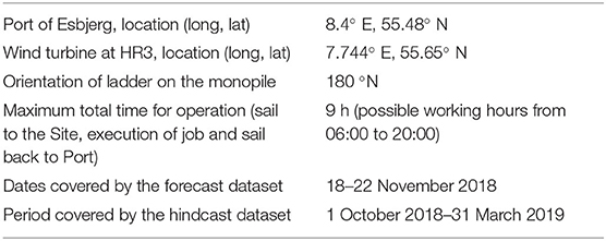
Table 1. Input used in the simulation for Port and Site location and forecast service.
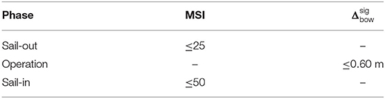
Table 2. Thresholds used to define the feasibility of the task for the three different phases.
Figure 2 depicts the domain used in the simulation, with the spatial discretization (mesh) and the bathymetry. The resolution of the mesh was finer in the Port area, i.e., 0.002 × 0.002° approximately, in order to properly represent the existing navigation channel. In the rest of the domain, the resolution was 0.020 × 0.020° approximately. It is noted that the available bathymetry dataset would have allowed the use of the finer resolution (0.002 × 0.002°) all over the domain, without increasing the computational demand of the tool significantly. Nevertheless, the lower resolution was employed in the offshore area for consistency with the resolutions of the available metocean datasets (presented below).
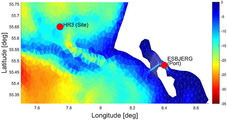
Figure 2. Spatial domain and mesh resolution adopted in the simulations. Color scale is for water depth in meter.
The following metocean forcings were applied as input in the simulations:
• Spectral significant wave height Hm0, Peak wave period Tp, and Mean Wave Direction (MWD) for both swell and sea component.
• Wind Speed (WS) and Wind Direction (WD)
• Surface Level (WL), Current Speed (CS), and Current Direction (CD).
This input was prepared in a pre-processing stage by interpolating the available dataset onto the mesh shown in Figure 2. Data was retrieved from open sources as follows:
• For wave data, the dataset NWS_004_014 from the Copernicus Marine Environment Monitoring Service (CMEMS) was applied2. This dataset had a spatial resolution of 0.016 × 0.016° and a temporal resolution of 1 h.
• For wind data, the data from the Climate Forecasting System Reanalysis (CFSR) was used (Saha et al., 2010). This dataset had a spatial resolution of 0.200 × 0.200° and a temporal resolution of 1 h.
• For tides and currents, the dataset NWS_004_013 was obtained from CMEMS (Tonani et al., 2019). This dataset had a spatial resolution of 0.016 × 0.016° and a temporal resolution of 1 h. Current speeds and directions provided at the sea surface level were used in this study.
The metocean conditions at the Site are displayed in Figures 3, 4. It can be seen that the current speed was moderate, with a tidal influence and with direction going to 200 °N and 350 °N. The wind speed was higher, i.e., 15 m/s, around the 21st, leading to a higher significant sea wave height on the same day (1.3 m). Sea peak wave period was around 3.5 s for most of the time. Swell peak period was 5 s approximately during the period with peaks at 18 s during the 18th afternoon and the 19th morning. As the time-variation of the mean wave direction reveals, swell waves came mainly from north until the 20th afternoon and mainly from south for the remainder of the forecast period. Sea waves came from north-east and east.
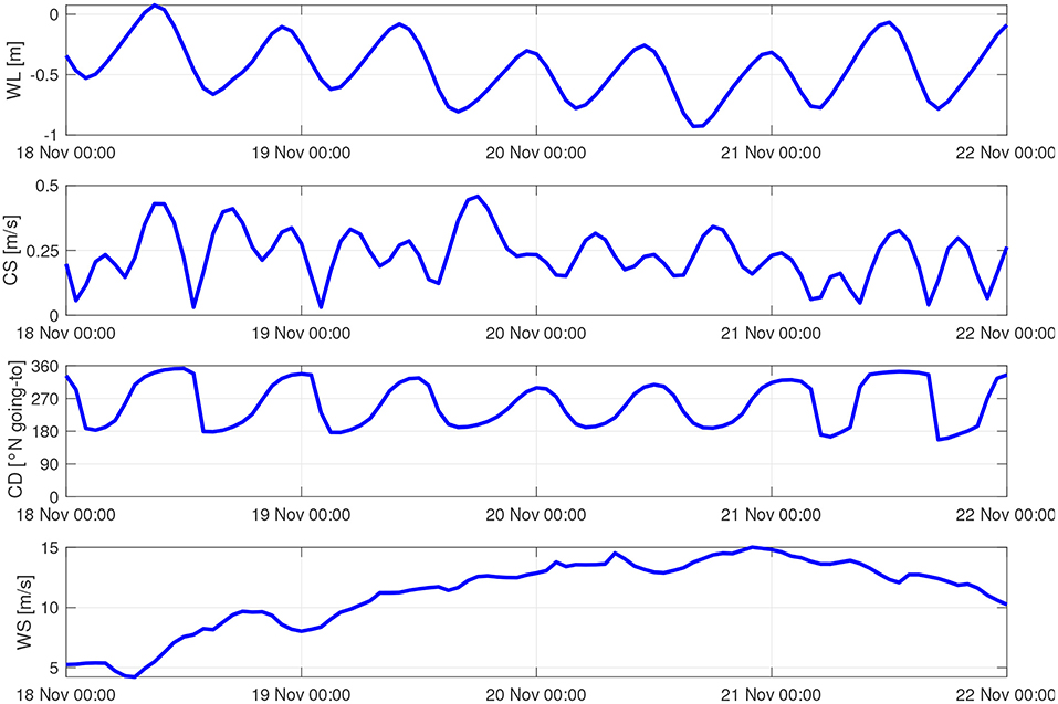
Figure 3. Time series of Water Level (WL), Current Speed (CS), Current Direction (CD), and Wind Speed (WS) extracted at the Site (see Figure 2) from the 5-day forecast dataset.
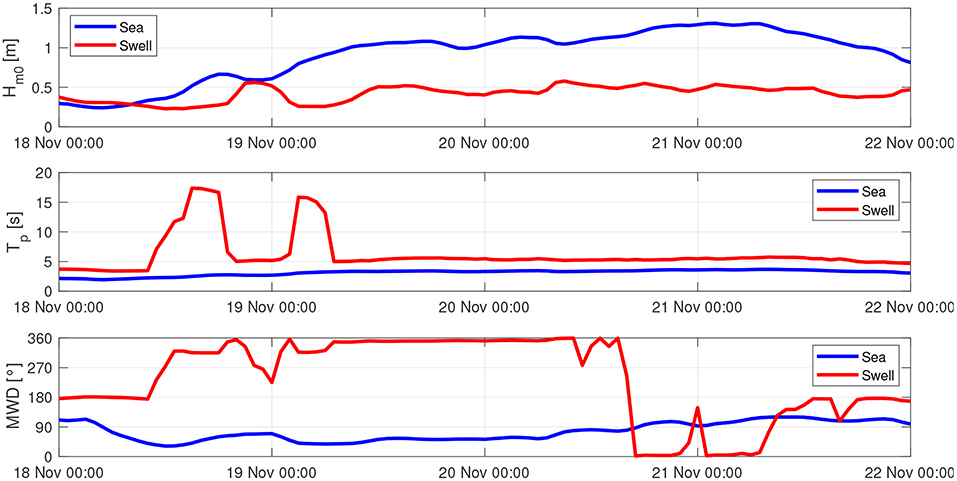
Figure 4. Time series of spectral significant wave height Hm0, peak wave period Tp, and Mean Wave Direction MWD extracted at the Site (see Figure 2) from the 5-day forecast dataset.
As already mentioned, the vessel used in this study was a CTV, which is a type of vessel widely used in the offshore wind sector to transfer personnel and equipment out to sites on a daily basis. In general, a CTV has dimensions and seakeeping characteristics designed to suit the O&M operations required by an OWF. The catamaran hull allows high speed, stability (e.g., low sensitivity to roll) and comfort onboard.
The CTV used in this study was 21 m long and 7.5 m wide approximately with a mean draft of 1.15 m. The 6DOF-rigid body motions of the CTV, induced by the wave forcing, were determined through the RAOs from S-Omega by FORCE Technology. The RAOs are in general a function of geometry of the hull, load onboard, water depth, vessel speed and heading. The geometry of the hull used by FORCE Technology is depicted in Figure 5. A realistic load onboard was assumed, that is 12 passengers. In order to account the variation with the other mentioned factors, the RAOs for surge, sway, heave, roll, pitch and yaw were provided at a discrete number of water depths (5 and 35 m), vessel speeds (0, 3, 6, 9, 12, 15, 18, and 21 knot), and vessel headings (0.0, 22.5, 45, 67.5, 90, 112.5, 135, 157.5, and 180°). As an example, Figure 6 gives an overview of the RAOs for heave, roll and pitch and their variation with water depth, vessel speed and heading.
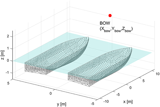
Figure 5. Hull of the CTV employed in the S-Omega simulations to derive the RAOs. The red marker is the reference point used as the bow (Xbow = 10.20 m, Ybow = 0 m, Zbow = 2.20 m).
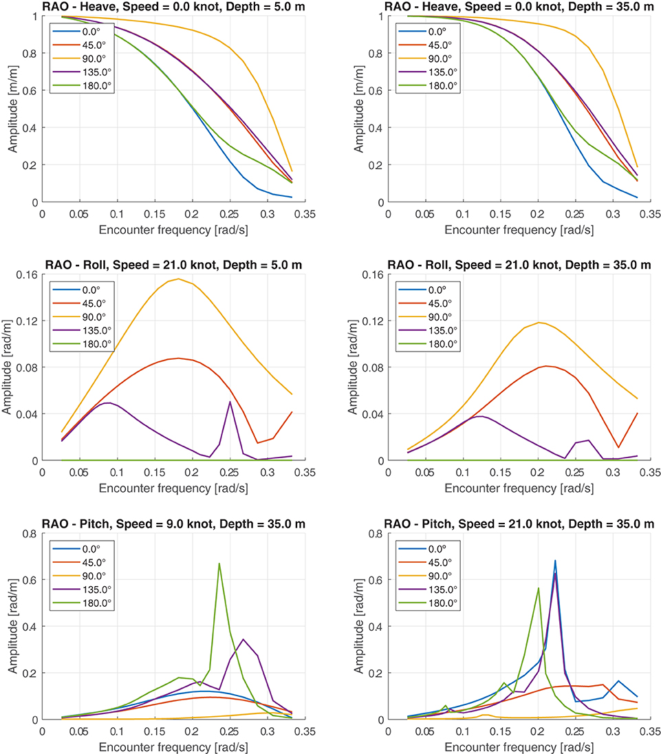
Figure 6. Response Amplitude Operator (RAO) for heave, roll and pitch of the employed CTV. The subplots give an overview of the sensitivity of RAOs to vessel speed, vessel heading, water depth, and encounter frequency.
At each time step, the tool interpolated the available RAOs linearly, according to vessel speed (relative to current speed), heading (relative to wave direction) and water depth. It is noted that the chosen discrete water depth values (5 and 35 m) covered the range of the actual depths in the whole domain (Figure 2). Moreover, those two values were sufficient to account for the variation of the RAOs with respect to the water depth. As it is possible to recognize in Figure 6, the water depth did not influence the vessel response largely, given the same speed and heading. This was due to the fact the draft of the CTV was very small compared to the bathymetry of the area.
The employed CTV was not prone to significant wind-induced motions, e.g., roll. In fact, the transverse surface of the hull, on which the wind would exert its force, was not large.
The route and the speed of the CTV were prescribed as in Figure 7, which displays a series of waypoints (long, lat) along with the corresponding speed of the vessel at those positions. It can be recognized that the CTV left the Port with a speed of 8 knot, then it accelerated up to 21 knot and kept this speed constantly until it reached the Site. It is noted that a speed of 21 knot was within the realistic operational range of the adopted CTV. At the Site, the CTV stopped for executing the task, i.e., speed was zero knot. After the operations, the CTV headed to the Port along the same track and with the same constant speed (21 knot). In the simulations, a new particle-vessel was generated and released at the Port every hour from 6:00 to 12:00. This meant a total of seven trips per each day of the simulation. This choice was made because the duration of the operation phase was 6 h. The total time required by the task was thus 8.5 h, which was within the assumed limit of 9 consecutive hours out in the sea for the CTV.
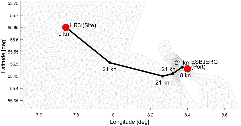
Figure 7. Prescribed track and speeds for the transfer of the CTV from the Port to the Site and then back to the Port.
4. Results and Discussions
The output of the simulation was time series of relevant parameters for each computed trip, which allowed a thorough assessment of workable conditions within the 5-day forecast period. As an example, two trips are analyzed in the following, because they represent well-recognized inefficient and risky situations that typically occur in the execution of O&M activities.
Figure 8 displays the output of the trip departed on the 21st of November 2018 at 07:00. In this trip, the MSI during the sail-out (and the sail-in) phase was not exceeded, but was higher than the threshold for the whole time at the Site. In other words, the CTV could sail to the Site without inducing significant seasickness, but no window for a safe transfer of the technicians on the mono-pile was actually available. If it had not been forecast, this trip would thus end up in either returning to the Port without accomplishing the job or a transfer on the mono-pile unsafe for the workers; both cases should be avoided in an efficient and safe planning of O&M tasks. In fact, a traditional weather window analysis assuming a maximum significant wave height and peak wave period of 1.5 m and 10 s, respectively, which are realistic thresholds often used in O&M planning, would assess this trip as feasible.
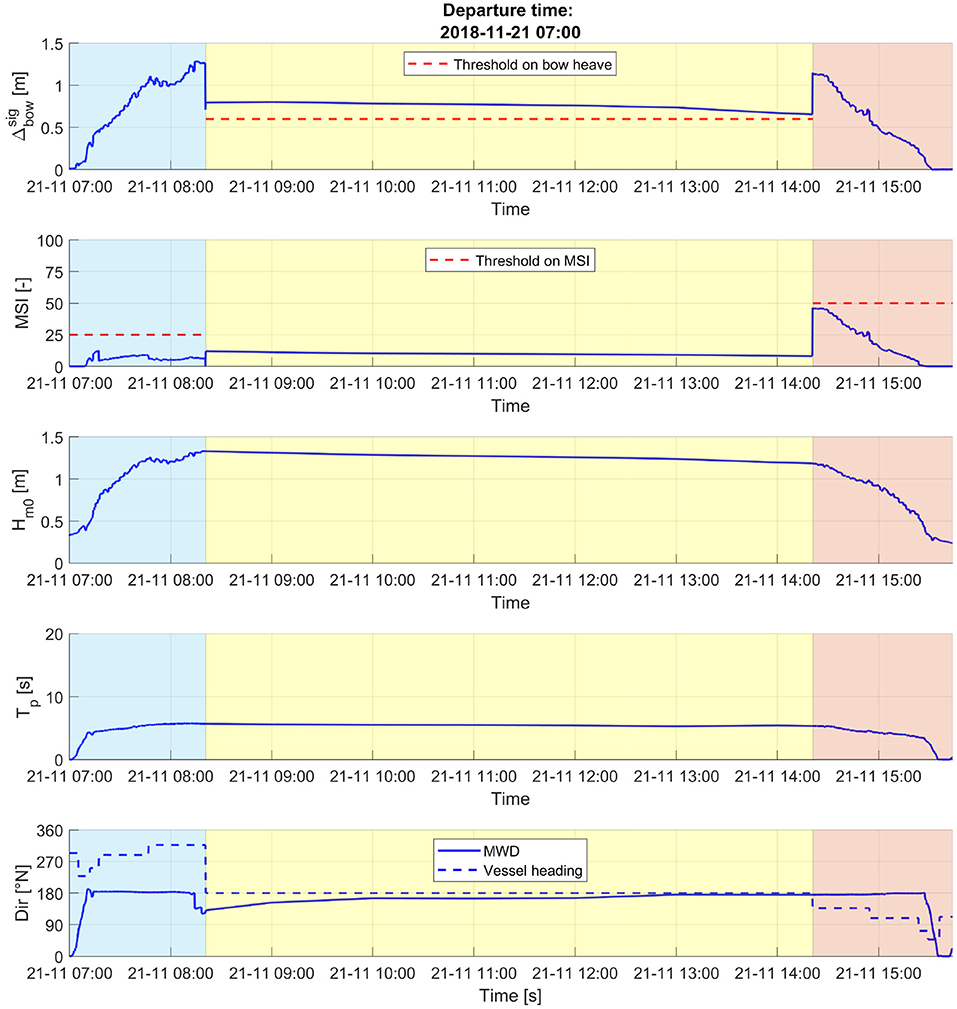
Figure 8. Output for the trip departed on the 21st of November 2018 at 07:00. From top to bottom panel: significant vertical displacement of the bow (), Motion Sickness Incidence (MSI), combined significant wave height (sea and swell), swell peak wave period, and swell mean wave direction. Bottom panel displays also the CTV direction. In each plot, the time window for each phase is marked with a different color, i.e., cyan for sail-out, yellow for operation, pink for sail-in.
Figure 9 displays the output of the trip departed the 19th of November 2018 at 11:00. In this trip, the MSI during the sail-out phase exceeded the threshold, while was within the limit. In this situation, it often happens that the workers on board of the CTV cannot start the operations because of seasickness, although the transfer on the mono-pile would be safe enough. Therefore, the operator needs to wait out at the sea until the technicians are finally able to work or, in the worst case scenario, the operator aborts the mission and sails back. It is again noted that a traditional weather window analysis with maximum significant wave height of 1.5 m and maximum peak wave period of 10 s would not reveal this risk.
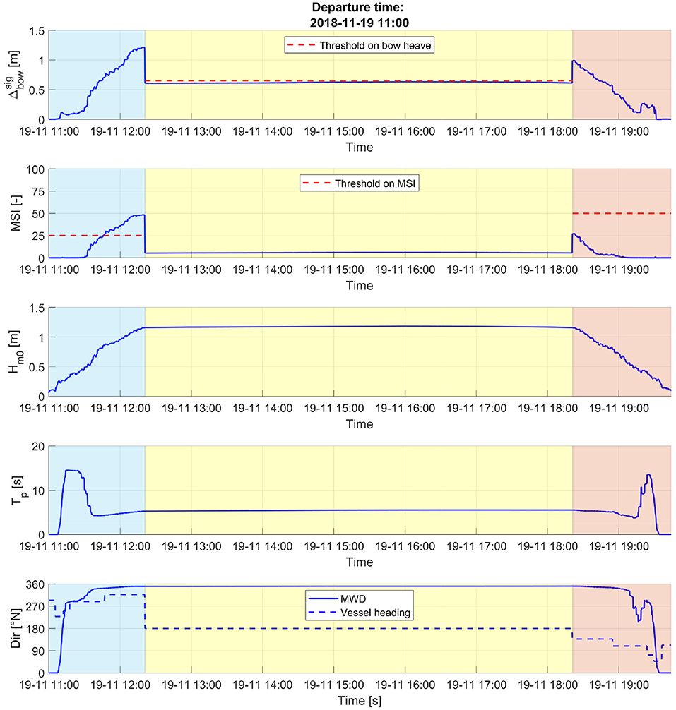
Figure 9. Output for the trip departed on the 19th of November 2018 at 11:00. From top to bottom panel: significant vertical displacement of the vessel bow (), Motion Sickness Incidence (MSI), combined significant wave height (sea and swell), swell peak wave period, and swell mean wave direction. Bottom panel displays also the CTV direction. In each plot, the time window for each phase is marked with a different color, i.e., cyan for sail-out, yellow for operation, pink for sail-in.
The results from all simulated trips were combined in order to find the time periods, during the whole 5-day forecast, suitable for the sail-out, the operation and the sail-in phase. The outcome of such an analysis is displayed in Figure 10, which would represent a great visual help for the O&M operator in planning the activities. As an example, the figure shows that the best days to execute the task are the 18th and the 22nd, because neither the transfer to the OWF (MSI) nor the workability at the Site () pose a risk for the execution of the task. Instead, there are no workable windows on either the 19th or the 20nd, because of the risk of seasickness (MSI ≥ 25) and the not safe conditions at the Site for the crew transfer ( ≥ 0.60 m). In the morning of the 21st, the trip to the OWF would be feasible, but the conditions at the Site are not fine for the work. This is a typical situation that occurs in O&M and it's a well-recognized source of inefficiency.
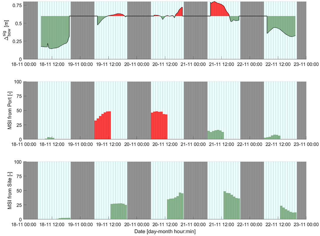
Figure 10. Weather windows for the 5-day forecast 18th–22nd November 2018. From top to bottom panel: significant vertical displacement of the vessel bow at the Site, maximum Motion Sickness Index (MSI) during the trip from the Port to the Site, maximum MSI during the trip from the Site to the Port. Green color indicates values below threshold, red color above threshold. Night hours are in gray, day hours in cyan.
The sensitivity of the tool to uncertainties of the metocean forecast was tested in the same scenario. Those uncertainties were artificially introduced by applying a ±10%-variation to each parameter contained in the 5-day forecast dataset (Hm0, Tp, MWD, WS, WD, WL, CS, and CD). The scenario was thus simulated again with the modified metocean forecast, while track, speeds, operation thresholds were kept identical. As expected, MSI and changed according to the new conditions, as the metocean input actually drives the response of the vessel. It was recognized that the workability prediction could turn in some of the hours during which MSI and were originally close to their threshold. As an example, working at the Site on the 19th between 16 and 17 turned to be feasible. Nevertheless, the overall weather window assessment did not differ much from the outcome shown in Figure 10. The capability of the tool to convert metocean conditions into actual workability criteria related to vessel motions can, to some extent, reduce the potential impact of forecast errors on weather window analyses.
As mentioned in the introduction of this paper, the aim of the tool is to provide weather windows more reliable than traditional workability assessments based on metocean conditions directly. In order to investigate the degree to which the tool has such capability, the application presented in section 3 was repeated on a 6 month-hindcast dataset (1 October 2018–31 March 2019). The same type of CTV (RAOs), track and speeds, which were used in the forecast application, were applied. The workability determined by the tool was compared with the predictions of the traditional approach. It is highlighted that the tool was set to initiate a new trip to the OWF every hour, which gave a total of 1,267 simulated trips during the investigated period. Therefore, the probabilistic comparison presented in the following was based on a large metocean and vessel response dataset. The chosen hindcast period allowed to compare the assessment of the tool and the traditional approach for the winter months, during which weather windows are expected to be infrequent and trustworthy predictions of workability are thus more critical than in the summer season. The output time series of metocean and vessel response parameters were elaborated as explained in the following.
A simulated trip was assessed feasible, either by the tool or the traditional approach, if both the transfer to the OWF (sail-out) and the operations at the Site were feasible. No constraints were applied on the sail-in phase. The tool applied thresholds on the Motion Sickness Incidence and the heave of the bow, i.e., MSILIM and , respectively. For the traditional approach, two different thresholds were applied on the significant wave height during the transfer and during the operations at the Site, i.e., and namely. A trip was thus defined successful when the following conditions occurred
where “(t)” indicates the time-variation of a parameter during the simulated trip.
Based on the conditions in Equation (12), a success rate was defined as the number of successful trips out of the 1,267 trips simulated during the 6 months period. The tool calculated such success rate per each of the combinations given by nine values of MSILIM (20–100 with 10-pace bins) and nine values of (0.2–1.0 m with 0.1 m-pace bins). Per each of those 81 combinations, an iterative procedure was applied to estimate a pair of thresholds - with which the traditional approach provided the same success rate. As an example, the tool calculated a 25% success rate with (MSILIM,) = (40, 0.6 m). With the traditional approach, the same success rate was obtained with (,) = (0.80, 1.0 m). With the known pairs of thresholds -, the predictions of the tool and the traditional approach were compared per each simulated trip as explained in the following. If a trip was successful for both the tool and the traditional approach, that trip was marked as “true positive.” If a trip was a failure for both methods, the trip was a “true negative.” With assuming the tool to give the trustworthy assessment, a trip was marked as a “false positive” if it was not feasible for the tool and feasible for the traditional approach. Likewise, a trip was a “false negative” if it was successful for the tool and a failure for the traditional approach. The differences in predictions of the two methods thus laid on either the “false positive” or the “false negative” trips. These trips induce the inefficiencies that the O&M industrial players experience and aim to minimize, as they represent situations in which either the CTV sails out without executing the job (false positive) or the CTV does not sail out, but the task could be accomplished (false negative). The amounts of “true” and “false” trips, either positive or negative, were finally divided by the total number of trips. The results of this analysis are shown in Figure 11. For each combination of thresholds, the gray bar represents the percentage of “true positive” trips; the colored bar on the top displays the sum of “false positive” and “false negative” trips. The percentage of “true negative” trips (not depicted) is the complementary to 100%. It can be observed that the predictions can differ by up to 12% when MSILIM is low (20–30) and is large (0.8–1.0 m). When MSI was not constrained, i.e., MSI = 100, the differences accounted for 5% approximately over the investigated values of .
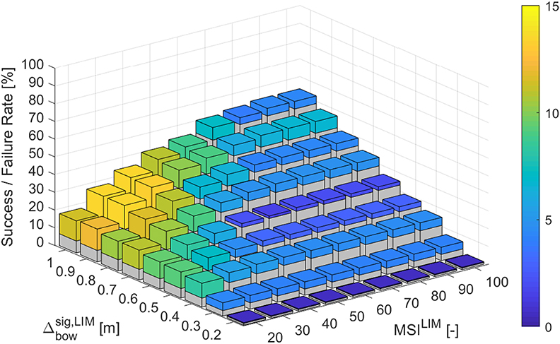
Figure 11. Results of the analysis for the hindcast 1st October 2018–31st March 2019. The gray bars represent the percentage of trips that are successful according to both the tool and the traditional approach, for different combinations of MSILIM and . Assuming MSI and to be the actual measures of workability, the colored bars represent the combined percentage of “false positive” and “false negative” trips. In those trips, the traditional approach failed the correct prediction, either assessing the O&M task feasible when it was not (“false positive”) or vice versa (“false negative”).
The tool and the traditional approach were further compared in the prediction of the most successful month over the hindcast period for the execution of the simulated O&M task. For this analysis, the tool applied MSILIM = 25 and = 0.60 m (as in section 3). The above-mentioned iterative procedure allowed to find the corresponding thresholds on the significant wave height for the traditional approach, i.e., = 0.70 m and = 1.0 m, giving the same success rate. The feasibility of all trips carried out in each month was assessed with both methods and the monthly success rates were derived. Results are shown in Figure 12. It can be observed that November was the most successful month according to both methods. Nevertheless, the traditional approach underestimated the success rate by 10% approximately. In December instead, the traditional approach overestimated the prediction of the tool by 7% circa. For the rest of the period, the two methods provided similar success rates.
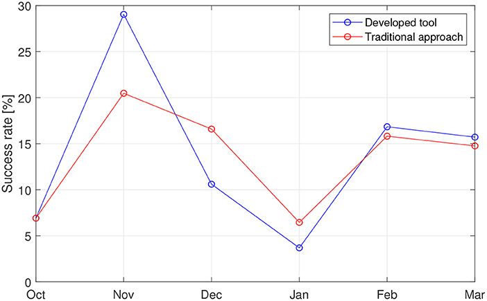
Figure 12. Results of the analysis for the hindcast 1st October 2018–31st March 2019. Monthly success rate over the investigated hindcast period predicted by the developed tool (blue line) and the traditional approach (red line).
As the route of the CTV was fixed throughout the whole simulated hindcast scenario, the sensitivity of the results of the tool to the chosen route was investigated. The hindcast scenario was then simulated again with changing the CTV route only, to potentially increase or decrease the impact of MSI in the long-term. With the original route, the CTV sailed northwesterly to the Site after leaving the Port. With the modified route, the vessel sailed first westerly and then northerly to reach the Site. It was found that the modified route decreased the success rates from October to January by 5% approximately, while the success rates did not change significantly in February and March. The comparison with the traditional approach, conducted as already described above, revealed again that the tool was more reliable in up to 12% of the predictions.
It is worth mentioning the computational demand of the developed tool. The simulation of the 5-day forecast took 2 min on one core of a standard laptop, while 1 h was necessary for the hindcast scenario. Such low computational time-demand is an important dimension in both forecast and hindcast scenarios and it is primarily due to the use of an ABM framework for modeling. This characteristic allows fast re-execution of the tool in daily operations, when a new forecast dataset is available as an example and to run the model with ensemble input allowing a probability of success to be defined for each start time.
5. Summary and Conclusions
This paper has presented a numerical tool for predicting weather windows with workable conditions for personnel operating O&M activities for OWFs. Traditionally, such weather windows come from analyses where time series of metocean parameters in the area of interest are compared with fixed thresholds, usually decided by O&M operator upon experience. The main aim of the study was to show how workability predictions can be different when based instead on direct measures of workability, that is seasickness during the trip to OWF or bow displacements that make the crew transfer from vessel to turbine mono-pile difficult.
An application of the tool in a 5 day-forecast scenario has been presented, where the execution of the O&M task was simulated together with the trip from the port to the OWF and back to port after the work. The study has shown the key capability of the tool of calculating the motions of the vessel employed in the operations. The vessel motions were used to produce two direct measures of the workable conditions, i.e., the significant vertical displacement of the vessel bow and the Motion Sickness Incidence. In particular, it has been presented how both outputs can support the decision-making process of the O&M operators, when one or more tasks should be accomplished in the coming working days and there is the need to decide if and when it is possible to sail out and come back safely.
The paper has also shown that the tool can be used with hindcast metocean databases, hence for simulations covering several months or years. This capability supports long-term seasonal plans when it is necessary to know, as an example, what is the likelihood that a specific task can be executed in a certain month as well as for cost estimation during design. The application in the hypothetical, but realistic, hindcast scenario enlightened the extent to which the predictions of the two methods, i.e., metocean conditions only or vessel motion-derived parameters, can differ. In fact, it was found that the traditional approach either overestimated or underestimated the workability in up to 12% of the predictions.
Future work will involve an extensive validation of the tool with a survey campaign during the execution of O&M tasks. The vessel motions, the metocean conditions and the feedback of the crew about workability will be measured and compared with the predictions of the tool. Furthermore, the numerical engine will include the adaptation of the route and the speed of the vessel to local adverse metocean conditions during the simulation. With such feature, it will be possible to flexibly minimize the impact of the weather conditions on the feasibility of the transfer to the offshore site, hence to potentially increase the availability of weather windows.
Data Availability Statement
Publicly available datasets were analyzed in this study. This data can be found at: for waves, current, and surface level data https://resources.marine.copernicus.eu/?option=com_csw&task=results. For wind data https://rda.ucar.edu/datasets/ds094.2/.
Author Contributions
PT was responsible for the development of the tool, the presented analyses, and for writing the draft of this paper. MD supervised the development of the tool and contributed to the presented analyses. RB assisted in the metocean data collection and reviewed the draft. JS proposed the idea of developing the presented tool and reviewed the draft. All authors contributed to the article and approved the submitted version.
Funding
This work has received funding from the European Union's H2020 Program for Research, Technological Development and Demonstration under Grant Agreement No: H2020-EO-2016-730030-CEASELESS.
Conflict of Interest
The authors declare that the research was conducted in the absence of any commercial or financial relationships that could be construed as a potential conflict of interest.
Footnotes
1. ^https://forcetechnology.com/en/services/seakeeping-evaluation
2. ^http://marine.copernicus.eu/services-portfolio/access-to-products/
References
Bolanos, R., Hansen, L., Rasmussen, M., Golestani, M., Mariegaard, J., and Nielsen, L. (2018). Coastal bathymetry from satellite and its use on coastal modelling. Coast. Eng. Proc. 1:98. doi: 10.9753/icce.v36.papers.98
Denis, M., and Pierson, W. (1953). On the motion of ships in confused seas. Trans. Society of Naval Architects and Marine Engineering. Defense Technical Information Center, 61, 280–354.
Hasselmann, K., Barnett, T., Bouws, E., Carlson, H., Cartwright, D., Enke, K., et al. (1973). Measurements of wind-wave growth and swell decay during the joint North sea wave project (JONSWAP). Deut. Hydrogr. Z. 8, 1–95.
Marsh, G. (2007). What price O&M? Operation and Maintenance costs need to be factored into the project costs of offshore wind farms at an early stage. Refocus 8, 22–27. doi: 10.1016/S1471-0846(07)70062-8
Neumann, J. V., and Burks, A. W. (1966). Theory of Self-Reproducing Automata. Urbana, MD: University of Illinois Press.
Newman, J. (1979). The theory of ship motions. Adv. Appl. Mech. 18, 221–283. doi: 10.1016/S0065-2156(08)70268-0
O'Hanlon, J., and McCauley, M. (1974). Motion sickness incidence as a function of vertical sinusoidal motion. Aerosp. Med. 45, 366–369.
Saha, S., Moorthi, S., Pan, H.-L., Wu, X., Wang, J., Nadiga, S., et al. (2010). The NCEP climate forecast system reanalysis. Bull. Am. Meteorol. Soc. 91, 1015–1058. doi: 10.1175/2010BAMS3001.1
Sanchez-Arcilla, A., Staneva, J., Cavaleri, L., Badger, M., Bidlot, J., Sørensen, J., et al. (2020). White paper the CMEMS coastal dimension. Conditioning, coupling and limits for applications. Front. Mar. Sci.
Seyr, H., and Muskulus, M. (2019). Decision support models for operations and maintenance for offshore wind farms: a review. Appl. Sci. 9:278. doi: 10.3390/app9020278
Keywords: offshore wind farm, Operation&Maintenance, decision-making, weather windows, vessel motions, O&M cost, O&M support, cost-efficiency
Citation: Tomaselli PD, Dixen M, Bolaños Sanchez R and Sørensen JT (2021) A Decision-Making Tool for Planning O&M Activities of Offshore Wind Farms Using Simulated Actual Decision Drivers. Front. Mar. Sci. 7:588624. doi: 10.3389/fmars.2020.588624
Received: 29 July 2020; Accepted: 11 December 2020;
Published: 12 January 2021.
Edited by:
Joanna Staneva, Helmholtz Centre for Materials and Coastal Research (HZG), GermanyReviewed by:
Bughsin Djath, Helmholtz Centre for Materials and Coastal Research (HZG), GermanyLichuan Wu, Uppsala University, Sweden
Copyright © 2021 Tomaselli, Dixen, Bolaños Sanchez and Sørensen. This is an open-access article distributed under the terms of the Creative Commons Attribution License (CC BY). The use, distribution or reproduction in other forums is permitted, provided the original author(s) and the copyright owner(s) are credited and that the original publication in this journal is cited, in accordance with accepted academic practice. No use, distribution or reproduction is permitted which does not comply with these terms.
*Correspondence: Pietro D. Tomaselli, ZHRvQGRoaWdyb3VwLmNvbQ==