Effects of Wind-Driven Lateral Upwelling on Estuarine Carbonate Chemistry

Estuaries are productive ecosystems that support extensive vertebrate and invertebrate communities, but some have suffered from an accelerated pace of acidification in their bottom waters. A major challenge in the study of estuarine acidification is strong temporal and spatial variability of carbonate chemistry resulting from a wide array of physical forces such as winds, tides and river flows. Most past studies of carbonate system dynamics were limited to the along channel direction, while lateral dynamics received less attention. Recent observations in Chesapeake Bay showed strong lateral asymmetry in the partial pressure of carbon dioxide (pCO₂) and air-sea CO₂ flux during a single wind event, but comparable responses to different wind events has yet to be investigated. In this work, a coupled hydrodynamic-carbonate chemistry model is used to understand wind-driven variability in the estuarine carbonate system. It is found that wind-driven lateral upwelling ventilates high DIC (Dissolved Inorganic Carbon) and CO₂ deep water and raises surface pCO₂, thereby modifying the air-sea CO₂ flux. The upwelling also advects low pH water onto the adjacent shoals and reduces the aragonite saturation state Ω_arag in these shallow water environments, producing large temporal pH fluctuations and low pH events. Regime diagrams are constructed to summarize the effects of wind events on temporal pH and Ω_arag fluctuations and the lateral gradients in DIC, pH, and pCO₂ in the estuary. This modeling study provides a mechanistic explanation for the observed wind-driven lateral variability in DIC and pCO₂ and reproduces large pH and Ω_arag fluctuations that could be driven by physical forcing. Given that current and historic mainstem Bay oyster beds are located in shallow shoals affected by this upwelling, a large fraction of the oyster beds (100–300 km²) could be exposed to carbonate mineral under-saturated $(\text{Ω}{}_{arag}<1)$ conditions during wind events. This effect should be considered in the management of acidification-sensitive species in estuaries.

Introduction

Riverine water typically has lower dissolved inorganic carbon (DIC) and total alkalinity (TA) values and a higher DIC/TA ratio than seawater (Salisbury et al., 2008; Huang et al., 2015; Cai et al., 2021). Because of this difference between the river and ocean end members, distributions of TA, DIC, pCO₂ (partial pressure of carbon dioxide), and pH in estuaries feature strong gradients in the along-channel direction (Cai and Wang, 1998; Borges and Gypens, 2010; Cai et al., 2011). In stratified estuaries, strong vertical gradients in DIC and pH also develop where phytoplankton photosynthesis in the surface euphotic layer consumes DIC and respiration of organic material in the bottom layer produces DIC (Feely et al., 2010; Cai et al., 2011, 2017). These strong horizontal and vertical gradients make estuarine carbonate chemistry susceptible to disruptions from physical forcing. Turbulent mixing generated by tides and winds may mix acidic bottom water upward, leading to large changes in the air-sea CO₂ flux (Cai et al., 2017; Paerl et al., 2018). Advection by tidal and wind driven currents across the horizontal gradient may cause large short-term pH fluctuations at fixed locations, which may add further stress to organisms for coping with extreme low pH events (Ribas-Ribas et al., 2013; Saderne et al., 2013; Pacellaa et al., 2018). There is an increasing recognition for the large temporal pH variability and extreme pH values in estuarine and coastal environments (Hofmann et al., 2011; Baumann et al., 2015; Baumann and Smith, 2018; Carstensen and Duarte, 2019), but most research has focused on metabolically driven pH fluctuations such as the diel photosynthesis/respiration cycle (Saderne et al., 2013; Baumann and Smith, 2018; Pacellaa et al., 2018). Relatively few studies have addressed how physical processes affect high-frequency carbonate chemistry in estuaries.

Wind-driven lateral upwelling is a well-known physical phenomenon in estuaries. Along-channel winds drive cross-channel transports via lateral Ekman transport in the surface layer of estuaries, leading to upwelling or downwelling flows at side boundaries and clockwise or counter-clockwise circulations in cross-channel sections. These lateral flows can transport momentum (Lerczak and Geyer, 2004; Scully et al., 2009), alter stratification (Lacy et al., 2003; Li and Li, 2011), and transport sediment (Geyer et al., 2001; Chen and Sanford, 2009). Using a numerical model of Chesapeake Bay, Li and Li (2012) found that the clockwise circulation generated under up-estuary winds is much stronger than the counterclockwise circulation generated under down-estuary winds. Xie et al. (2017) analyzed long-term mooring data at a cross-channel section in Chesapeake Bay and found that the lateral circulation strength increased linearly with wind speeds under up-estuary winds but was a parabolic and weaker function of wind speeds under down-estuary winds.

Wind-driven lateral circulation and upwelling can transport biologically important materials such as nutrients and oxygen between the deep channel and shallow shoals (Malone et al., 1986; Sanford et al., 1990; Reynolds-Fleming and Luettich, 2004; Wilson et al., 2008). In Chesapeake Bay, Malone et al. (1986) observed higher phytoplankton production over the flanks of the main channel relative to production over the channel and attributed it to nutrient exchanges by the lateral circulation. Episodic upwelling of hypoxic water from the deep channel to shallow shoals has been observed in several estuaries, including Mobile Bay (Loesch, 1960), the Neuse River (Eggleston et al., 2005), Long Island Sound (Wilson et al., 2008), and Chesapeake Bay (Sanford et al., 1990; Breitburg, 1992). These upwelling events have the potential to generate short-lived, but severely negative conditions for organisms residing in these otherwise favorable shallow habitats, where in extreme cases, flurries of organisms congregate near shorelines as the escape to the upwelled waters (e.g., a crab “jubilee”). In a modeling study of Chesapeake Bay, Scully (2010) showed that wind-driven lateral exchange of oxygen between well-oxygenated shallow shoals and hypoxic deep channel may be more important than direct turbulent mixing in supplying oxygen to the hypoxic deep channel.

CO₂ dynamics often mirror O₂ dynamics, since all chemical species are advected or diffused by the same physical processes (currents and mixing) while the production and consumption of DIC and O₂ are affected by common biological processes such as phytoplankton production and organic matter respiration. However, while surface-water O₂ equilibrates with the atmospheric concentration relatively quickly, surface-water pCO₂ is slow to adjust and rarely reaches equilibrium with respect to the atmospheric pCO₂ due to the buffering effect of a much greater DIC pool on aqueous CO₂ (Cai et al., 2020, 2021). Thus the effects of short-term wind effects may be different between O₂ and CO₂. Huang et al. (2019) made repeated measurements of temperature, salinity, and pCO₂ in surface waters at a cross-channel transect in the middle reach of Chesapeake Bay. They observed large temporal and spatial variations of pCO₂ during a northerly wind event. The air-sea CO₂ flux over the eastern one-third of this transect was 20–40% higher than the flux over the middle section whereas the CO₂ flux over the western one-third of this transect was 30% lower. Huang et al. (2019) hypothesized that northerly (down-estuary) winds generated upwelling on the eastern shore, enhancing the release of respired CO₂ from acidic subsurface water. This raises a question whether southerly (up-estuary) winds will generate higher pCO₂ on the western shoal and under what wind conditions this lateral upwelling mechanism is effective in generating the lateral asymmetry in the CO₂ flux. A related question is how this wind-driven lateral upwelling affects the overall carbonate chemistry in an estuary.

Our study site, Chesapeake Bay, is an ideal system to address these questions, given that it is a large eutrophic estuary with relatively low buffer capacity (Cai et al., 2017) and wind forcing is comparable to tidal forcing (Zhong and Li, 2006; Figure 1A). It stretches for about 320 km from the mouth of the Susquehanna River at Havre de Grace, Maryland to its seaward end at Cape Charles and Cape Henry, Virginia. It is shallow, with a mean water depth of 6.5 m. However, a deep paleochannel running in the north-south direction dominates the bathymetry in the middle reaches of the main Bay. Chesapeake Bay is a partially mixed estuary: vertical salinity differences of 2–8 stratify the water column (Carter and Pritchard, 1988). It features a two-layer circulation with speeds on the order of 0.1 m s⁻¹ (e.g., Goodrich and Blumberg, 1991). Compared with other estuaries, tidal forcing in the Bay is relatively modest with tidal range rarely exceeding 1 m (Browne and Fisher, 1988). Winds are episodic with dominant periods of 2–7 days.

FIGURE 1

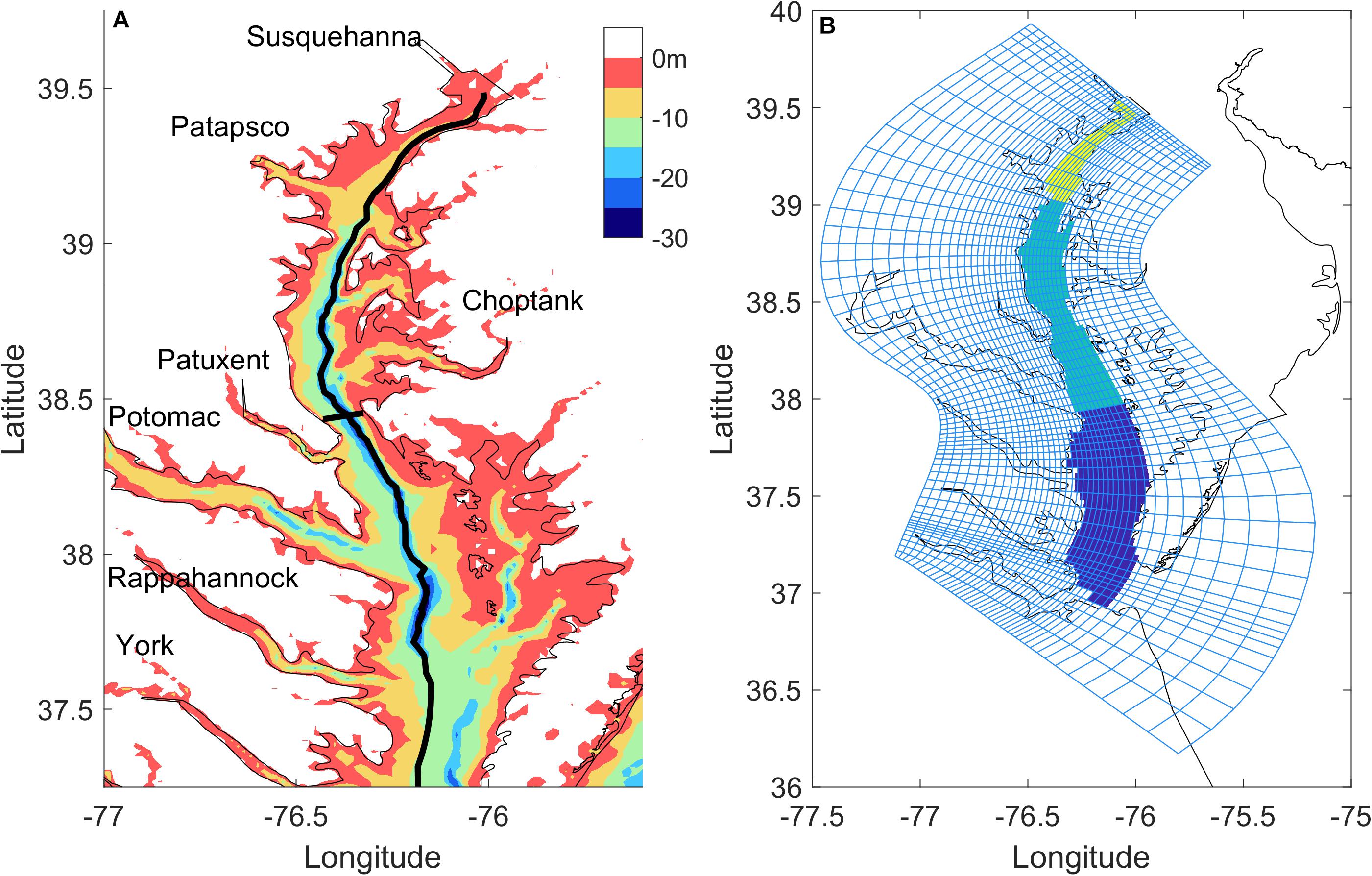
Figure 1. Map showing bathymetry (A) and model grids (B) for Chesapeake Bay. The black lines in (A) marks the along-channel section and a cross-channel section in the mid-Bay used in later analysis. The shaded areas in (B) represent the upper, middle, and lower-Bay regions.

Recent observations have mapped out the distributions of DIC, TA, pCO₂, and pH in the main stem of Chesapeake Bay (Brodeur et al., 2019; Friedman et al., 2020). DIC and TA increased from surface to bottom and from north to south over the course of 2016. Upper, mid-, and lower bay DIC and TA ranged from 1000 to 1300, 1300 to 1800, and 1700 to 1900 μmol kg^–1, respectively. The pH range was large, with the maximum value of 8.5 at the surface and the minimum as low as 7.1 in bottom water in the upper and mid-bay (Brodeur et al., 2019). Significant spatial variability of pCO₂ was observed throughout the mainstem, with net uptake of atmospheric CO₂ during each season in the middle Bay and weak seasonal outgassing of CO₂ near the outflow to the Atlantic Ocean (Chen et al., 2020; Friedman et al., 2020). High-frequency pH data from a moored sensor showed high frequency fluctuations of DIC, pH, and pCO₂ influenced by circulation and biological processes (Shadwick et al., 2019). Coupled hydrodynamic-biogeochemical-carbonate chemistry models (ROMS-RCA-CC) have been developed for Chesapeake Bay (Shen et al., 2019a). Shen et al. (2019a) focused their modeling analysis on the large-scale carbonate chemistry dynamics and validation against field observations. Furthermore, Shen et al. (2019b) and Shen et al. (2020) conducted 30-year hindcast simulations to examine ecosystem metabolism and carbon balance and investigated the anthropogenic impacts on pH and aragonite saturation state. This modeling study takes the next step to investigate how physical processes affect carbonate chemistry in this estuary, seeking to test the lateral upwelling mechanism over a range of wind conditions, in particular during the up-estuary wind condition not observed in Huang et al. (2019). It also builds upon previous studies of O₂ dynamics to further our understanding of CO₂ dynamics.

Materials and Methods

To investigate how winds affected carbonate chemistry in Chesapeake Bay, we used coupled hydrodynamic-biogeochemical-carbonate chemistry models to conduct hindcast simulations. The coupled models have three sub-models. The hydrodynamic model, based on the Regional Ocean Modeling System (ROMS, Shchepetkin and McWilliams, 2005; Haidvogel et al., 2008), has 80 × 120 grid points (∼1 km resolution) in the horizontal direction and 20 vertical sigma layers, as shown in Figure 1B (Li et al., 2005). ROMS simulates water level, currents, temperature and salinity. The biogeochemical model is based on the Row-Column Aesop (RCA) model, and includes a water-column component (Isleib et al., 2007) and a sediment diagenesis component (Di Toro, 2001). RCA simulates pools of organic and inorganic nutrients, two phytoplankton groups, and dissolved oxygen concentrations (Testa et al., 2014). The carbonate chemistry (CC) model simulates DIC, TA, and mineral calcium carbonate (aragonite CaCO₃) (Shen et al., 2019a,b, 2020). DIC is consumed by phytoplankton growth/photosynthesis and calcium carbonate precipitation. The sources of DIC include air-sea CO₂ flux, phytoplankton respiration, oxidation of organic matter, calcium carbonate dissolution, sulfate reduction, and sediment-water fluxes. Calcium carbonate dissolution and precipitation is the primary source/sink for TA, but the contributions of several other biogeochemical processes (e.g., nitrification and sulfate reduction) to TA are also modeled (Shen et al., 2019a). Other carbonate chemistry parameters such as pH and pCO₂ are calculated from the CC model outputs using CO2SYS program (Lewis and Wallace, 1998).

The ROMS hydrodynamic model is forced by river flows at eight major tributaries, by wind stress and heat fluxes across the sea surface, and by sea level and climatology of temperature and salinity at the open boundary (Li et al., 2005, 2015; Cheng et al., 2013; Xie and Li, 2018). At the upstream boundary of the eight major tributaries, freshwater inflows measured at USGS gauging stations were prescribed. Tidal forcing at the open ocean boundary was decomposed into tidal constituents from TPXO7 (TOPEX/Poseidon) data-assimilative global tidal model (Egbert and Erofeeva, 2002). For non-tidal forcing at the offshore boundary, de-tided daily sea-level observations acquired at NOAA Duck station were used. Air-sea momentum and heat fluxes were computed by applying standard bulk formulae (Fairall et al., 2003) to NARR (North America Regional Reanalysis from National Center for Environmental Prediction) products.

The RCA biogeochemical model is forced by loads of dissolved and particulate materials from the eight major rivers. Riverine constituent concentrations for phytoplankton, silica, particulate and dissolved organic carbon, phosphorus, and nitrogen, and inorganic nutrients (ammonium, nitrate, phosphate) were obtained or derived from Chesapeake Bay Program biweekly monitoring data¹ as described in Testa et al. (2014). The ocean boundary concentrations were acquired from the World Ocean Atlas 2013 and Filippino et al. (2011). Atmospheric deposition was not considered.

The CC carbonate chemistry model is forced by the atmospheric CO₂, the riverine loads and offshore concentration of TA and DIC. Time series of TA measurements in riverine inputs were obtained from the USGS station in the Susquehanna and Potomac Rivers (Raymond et al., 2000). The riverine DIC concentrations were calculated through CO2SYS with the available TA and pH (Shen et al., 2020). The computed DIC is in very good agreement with the observed DIC when direct DIC measurements were made during the field cruises of 2016 (Supplementary Figure S1). Carbonate chemistry data for the other smaller tributaries were estimated using empirical relationships as functions of freshwater discharge (Shen et al., 2019a). TA at the ocean boundary was directly estimated with the empirical equation based upon salinity and temperature at the ocean boundary (Cai et al., 2010). DIC at the offshore boundary was calculated with the available TA, fCO₂ from SOCAT (Bakker et al., 2016), salinity and temperature using CO2SYS. The atmosphere pCO₂ was set to be 400 ppm.

Regional ocean modeling system was initialized with outputs from a hindcast simulation from 1 January to 31 December 2012. The initial conditions of RCA were based on Chesapeake Bay Program monitoring data in December 2012. Initial conditions for DIC and TA were calculated from the two-end member mixing model. Model hindcast simulation for this study lasted from 1 January to 31 December 2013.

The ROMS-RCA-CC models have been validated against a wide variety of observational data (e.g., Li et al., 2005, 2006, 2016; Zhong and Li, 2006; Testa et al., 2014; Xie and Li, 2018; Shen et al., 2019a,b, 2020; Ni et al., 2020). The ROMS hydrodynamic model has been validated against water level measurements at tidal gauge stations (Zhong and Li, 2006; Zhong et al., 2008), salinity and temperature time series at monitoring stations (Li et al., 2005; Ni et al., 2020), salinity distributions collected during hydrographic surveys, and current measurements (Li et al., 2005). In particular, Xie and Li (2018) showed that ROMS reproduced the wind-driven lateral circulation patterns, including the current field and salinity distribution at a cross-channel section in the mid-Bay. The RCA biogeochemical model has been validated against biogeochemical data at a number of stations in Chesapeake Bay (including NO₃, PO₄, NH₄, chlorophyll-a, dissolved oxygen, and organic carbon, nitrogen, and phosphorus), integrated metrics of hypoxic volume, rates of water-column primary production and respiration, and nutrient fluxes across the sediment-water surface (Brady et al., 2013; Testa et al., 2013, 2014, 2017; Li et al., 2016; Ni et al., 2020). The CC model has been validated against extensive surveys of DIC, TA, and pH collected during ten cruises in 2016 (Shen et al., 2019a) and long term (1985–2015) measurements of pH at a number of monitoring stations (Shen et al., 2019b, 2020). The model-predicted along-channel distribution of air-sea CO₂ flux is also in good agreement with that calculated from the observational data (Shen et al., 2019a). This paper uses the well-validated coupled hydrodynamic-biogeochemical-carbonate chemistry models to investigate how winds affect carbonate chemistry in this estuary.

Results

We examined the effects of up-estuary and down-estuary winds on lateral upwelling and carbonate system variability. Detailed modeling analysis revealed that interactions between wind direction and bathymetry determined the strength of upwelling and the associated bottom-surface exchange of low-pH and high-pCO₂ water. Regime diagrams were constructed to summarize the wind effects on carbonate system in the estuary and support a discussion of the associated impacts on Maryland’s oyster beds.

An example sequence of a southerly wind event followed by a northerly wind event illustrated the contrasting responses of pH to winds. Southerly (up-estuary) winds blew over Chesapeake Bay between 22.00 LST (Local Standard Time) 18 September and 6.00 LST 22 September 2013, with a maximum wind speed of ∼7.5 m s^–1 (Figure 2A). This was followed by northerly (down-estuary) winds between LST 6.00 on 22 September and LST 0.00 on 25 September 2013, with a maximum wind speed of ∼7.3 m s^–1. Figures 2B–D show how the surface and bottom water pH responded to winds at three locations (the western shoal, central deep channel, and the eastern shoal) in a mid-Bay cross section. During the up-estuary wind event, the surface/bottom pH on the western shoal decreased from 8.1/7.9 to 7.9/7.7 while pH on the eastern shoal increased from 8 to 8.2 (Figures 2B,D). During the following down-estuary wind event, the opposite trend appeared: the surface/bottom pH on the western shoal increased from 7.9/7.8 to 8.2/8.1 while pH on the eastern shoal decreased from 8.1 to 7.9. In the deep channel, the bottom pH was much lower than the surface pH and the vertical pH difference decreased from ∼0.6 to ∼0.4 during the strong winds (21–23 September) (Figure 2C). The differences in the pH time series at the three locations highlight the short-term variations in pH and carbonate chemistry in the estuary in response to wind forcing. Thus, we conducted a series of model simulations to quantify the carbonate system response to (a) weak winds, (b) up-estuary winds, and (c) down-estuary winds.

FIGURE 2

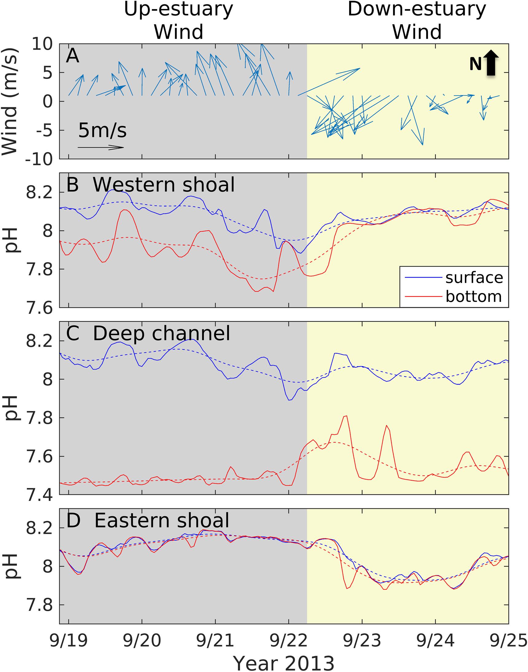
Figure 2. Time series of wind speed vector (A), surface (blue) and bottom (red) pH at a location on the western shoal (B), in the center channel (C), and on the eastern shoal (D) in a mid-Bay section (marked as black line in Figure 1A). The three locations are further marked as red dashed lines in Figure 4D. The solid lines are original time series including tidal fluctuations and the dashed lines are low-passed with a 34-h Butterworth filter.

Weak Wind

As a baseline for comparison, we plot the distributions of physical and carbonate chemistry fields during a period when wind speeds were below 2 m s^–1, e.g., 22.00 LST 3 October – 10.00 LST 5 October (Figures 3, 4). The tidally averaged current displayed a typical two-layer gravitational circulation, with seaward flow in the surface layer down to ∼10 m and landward flow in the underlying bottom layer (Figure 3A). The along-channel salinity distribution showed sloping isohalines typical of a partially mixed estuary, with the top-bottom salinity difference reaching ∼6 in the deep mid-Bay (Figure 3B). DIC and TA showed a similar along-channel distribution (Figures 3C,D). However, DIC had a larger vertical gradient than TA since phytoplankton production consumed DIC in the surface euphotic layer and respiration of organic material produced DIC in the bottom layer. The relative impacts of primary production and respiration on TA are small as is expected. pH also showed a strong longitudinal gradient, with lower pH values in the upper Bay due to the influence of poorly buffered, high-CO₂ riverine water and higher pH values in the lower Bay due to well-buffered oceanic water (Figure 3E). In addition, pH had a strong vertical gradient, with the top-to-bottom pH difference reaching 0.8 in the upper part of the mid-Bay. The aragonite saturation state Ω_arag showed a similar along-channel distribution as pH, falling below 1 in the upper Bay and bottom waters of the mid-Bay but reaching 2–3 in the surface waters of the mid-Bay and everywhere in the lower Bay (Figure 3F). The surface pCO₂ exceeded atmospheric equilibrium value in the upper Bay (north of 39.2°N), was undersaturated in the mid-Bay (37.5–39.2°N), and reached a near-equilibrium status in the lower Bay (south of 37.5°N) (Figure 3G). Consequently, the air-sea CO₂ flux showed outgassing of ∼5 mmol C m^–2 d^–1 in the upper Bay, and ingassing of (3–4) mmol C m^–2 d^–1 in the mid-Bay and near-zero exchange in the lower Bay (Figure 3H). When integrated over the main stem of the Bay, there was a net influx of −10.5×10⁶gCd⁻¹ into the estuary.

FIGURE 3

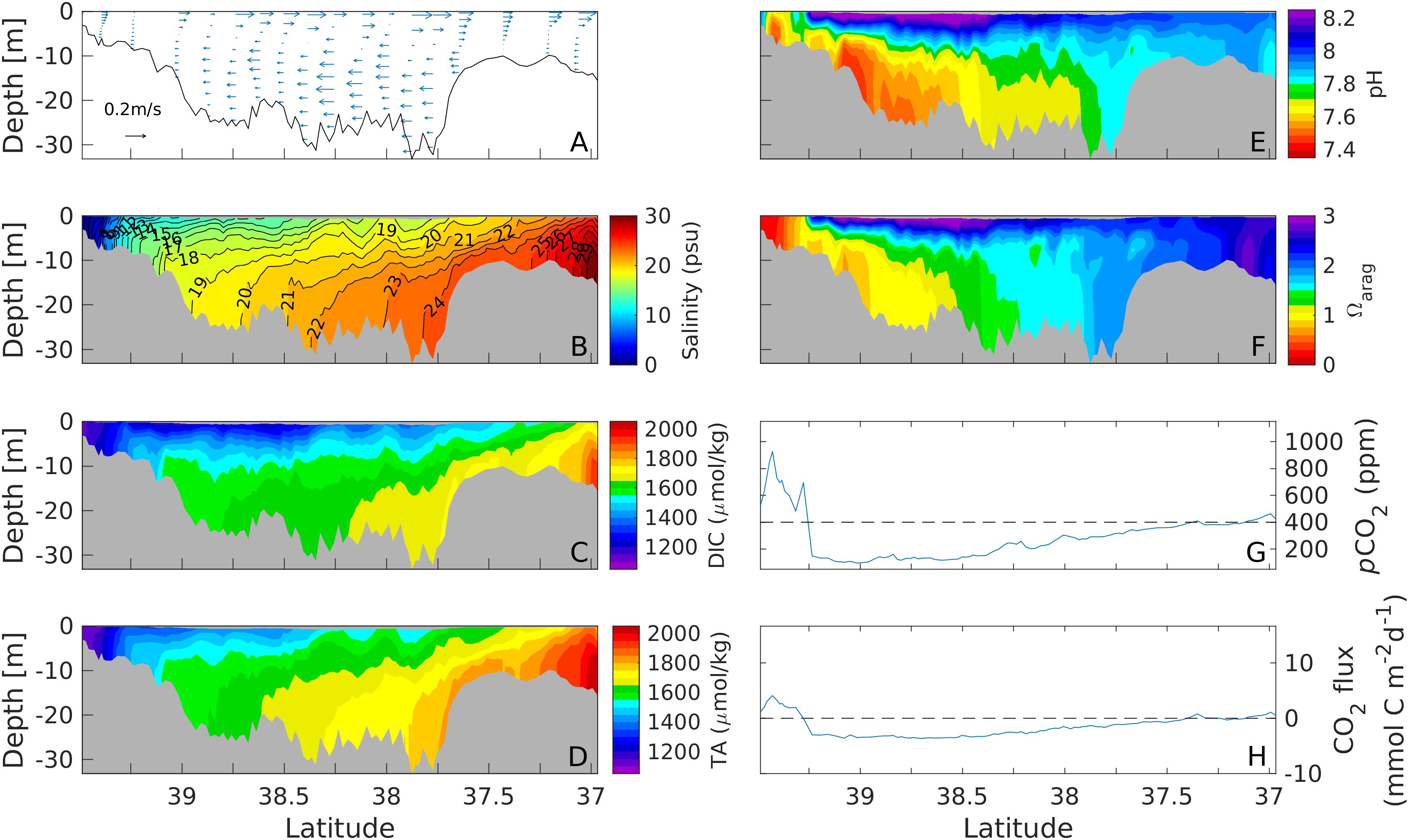
Figure 3. Along channel distributions of subtidal current (A), salinity (B), DIC (C), TA (D), pH (E), Ω_arag (F), surface pCO₂ (G), and air-sea CO₂ flux (H) during a weak wind period on 2–5 October, 2013. The along-channel section is marked by the black line in Figure 1A.

FIGURE 4

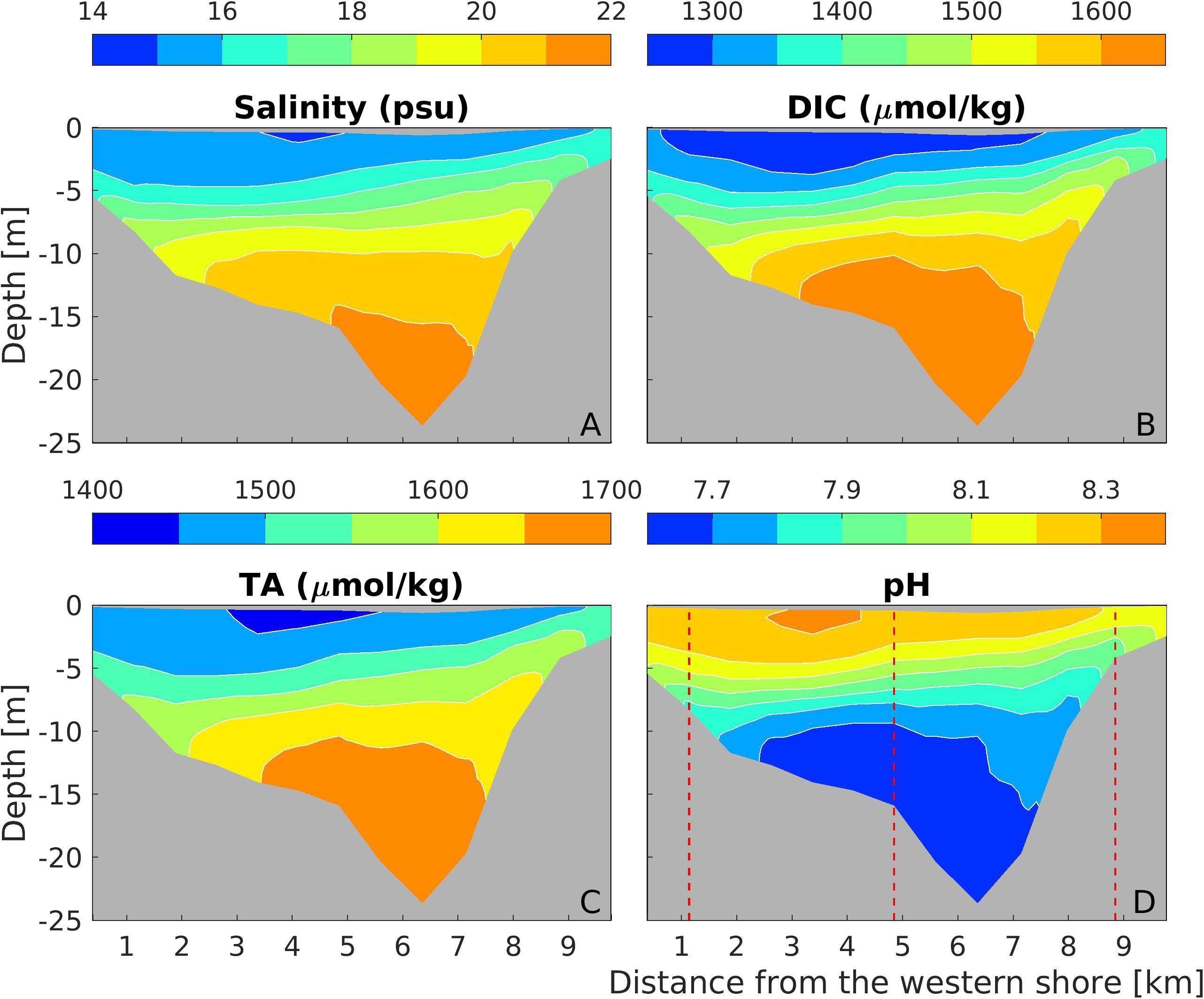
Figure 4. Distributions of salinity (A), DIC (B), TA (C), and pH (D) at a mid-bay cross section (marked as the thick black line in Figure 1A) during the weak wind period. The red dashed lines in (D) mark the three stations used for plotting pH time series in Figures 2B–D.

Since deep water in the mid-Bay is most susceptible to low pH and low O₂ in the estuary (Brodeur et al., 2019; Shen et al., 2019a), we examined a representative cross-channel section in this region. Salinity was vertically stratified and tilted slightly downward on the western shore as the Coriolis force confined the outflowing brackish water to the west (Figure 4A). DIC and TA also showed strong vertical gradients and a slight west-east tilt (Figure 4B), with lower DIC and TA within the western surface waters. pH isolines were also slightly tilted, but the lateral gradient in pH (∼0.2) was much smaller than the vertical gradient (∼0.7; Figure 4D).

Up-Estuary Wind

Winds led to large changes in the carbonate system. The up-estuary winds forced water in the shallow lower Bay to move landward at all depths (Figure 5A). In the deep mid-Bay, the currents moved landward in the surface layer whereas the pressure gradient due to sea level pileup at the head of the estuary drove the bottom water seaward, thereby reversing the gravitational circulation. This reversed circulation strained the salinity field toward the vertical direction, promoting the ventilation of deep water. Furthermore, wind-driven turbulence generated a surface mixed layer, with its depth reaching ∼10 m between 38.5 and 39°N (Figure 5B). The vertical mixing and along-channel straining also strongly modified DIC and TA fields (Figures 5C,D). Their vertical gradients were greatly reduced, with nearly a uniform distribution down to a depth of 10–15 m. In the mid and lower Bay, pH was separated into two regions in the vertical direction (8–8.2 in the surface layer and 7.4–7.6 in the bottom layer) and was uniform (7.4) at all depths in the upper Bay (Figure 5E). The aragonite saturation state also showed a sharp contrast between the surface and bottom layers, with highly under-saturated conditions in the bottom layer of the mid-Bay. The seaward flows in the bottom layer (Figure 5A) – which under these wind conditions were opposite of the direction of mean flows (landward) – advected the under-saturated bottom water further seaward in the mid-Bay (Figure 5F).

FIGURE 5

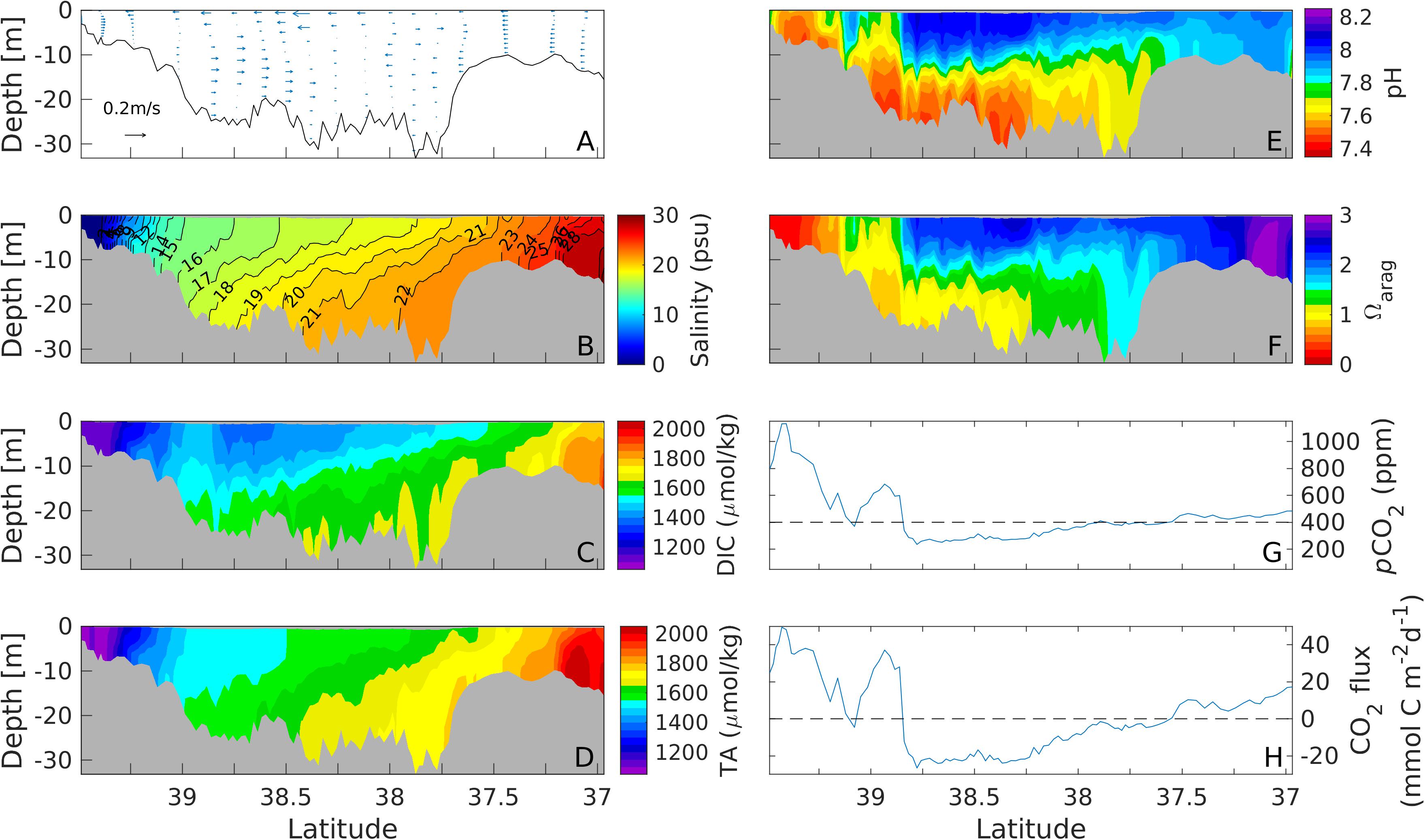
Figure 5. Along channel distributions of subtidal current (A), salinity (B), DIC (C), TA (D), pH (E), Ω_arag (F), surface pCO₂ (G), and air-sea CO₂ flux (H) during an up-estuary wind event on 18–22 September, 2013.

The southerly winds also impacted pCO₂ and air-sea fluxes. The surface water pCO₂ increased significantly in the mid-Bay as mixing and straining during the wind event raised the surface DIC (Figure 5G). Around 39°N, where bathymetry deepens rapidly, ventilation of the bottom water occurred, mixing high DIC-water upward and raising the surface water pCO₂ above atmospheric equilibrium. As a result, the peak in CO₂ efflux at 39°N rivaled the peak in the uppermost part of the Bay (>39.5°N) (compare Figures 3H, 5H). The wind event thus drove outgassing of CO₂ over an extended region in the upper and mid-Bay (down to 38.8°N), with a magnitude of 40 mmol C m^–2 d^–1. Further south in the wide mid-Bay (between 38.8 and 37.5°N), however, the estuary absorbed CO₂ at −20 mmol C m^–2 d^–1. When integrated over the entire estuary, there was a net influx of −12.1×10⁶gCd⁻¹.

The up-estuary winds also drove a strong clockwise lateral circulation in the cross-channel section, with the eastward velocity in the near-surface layer reaching 0.1 m s^–1 (Figure 6A). This resulted in upwelling on the western shore, with an upwelling velocity up to 0.5 mm s^–1. Consequently, isohalines were tilted upward on the western part of the cross-section (Figure 6B). Wind-driven turbulent mixing also homogenized salinity in the top 5 m. DIC and TA showed a similar upward tilt on the western shore, with the upwelling of high DIC and TA bottom water onto the broad western shore (Figures 6C,D). The upwelling changed acidity on the shallow shoals, where pH on the western shore was lowered (Figure 6E), reaching minima of 7.5–7.7 during the up-estuary wind (on the sea bed).

FIGURE 6

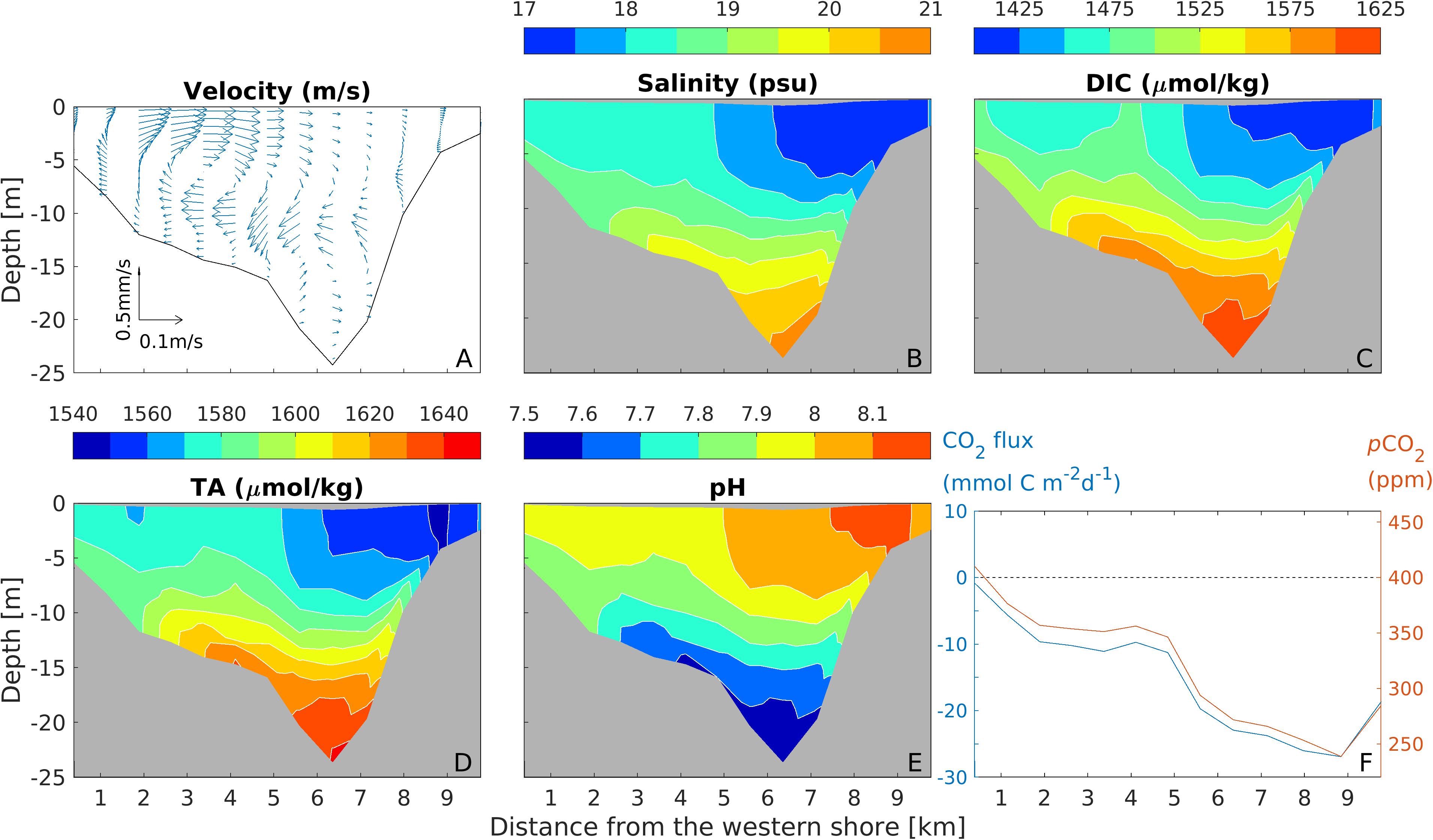
Figure 6. Distributions of lateral-vertical velocity vector (A), salinity (B), DIC (C), TA (D), pH (E), and surface pCO₂ (red) and air-sea CO₂ flux (blue) (F) and at the mid-bay section during the up-estuary wind event.

The upwelling resulted in much higher pCO₂ value on the western shore (∼350–400 ppm) than on the eastern shore (∼250 ppm). This lateral difference in the surface-water partial pressure led to a strong lateral gradient in the CO₂ flux (Figure 6F). The mid-Bay region has been identified as a carbon sink on an annual scale. During this up-estuary wind event, the surface pCO₂ on the western shore increased, resulting in weak CO₂ flux there. On the other hand, the CO₂ flux on the eastern part of the cross section increased to −30 mmol C m^–2 d^–1, producing a strong carbon sink. No significant change (<2 mg/L in chlorophyll a) in phytoplankton biomass was seen during the wind event (Supplementary Figure S2).

Down-Estuary Wind

Following the up-estuary wind event, northerly winds blew down the estuary (Figure 2A), with the maximum wind speed of 7 m s^–1. The down-estuary winds amplified the two-layer gravitational estuarine circulation, with the landward bottom current reaching 0.2 m s^–1 (Figure 7A). This strong two-layer current strained the salinity field to flatten the isohalines, while the direct wind-induced mixing homogenized salinity in the surface layer down to 10 m (Figure 7B). The landward flow in the bottom layer brought in higher salinity oceanic water into the estuary. This intrusion also caused bottom DIC and TA to increase (Figures 7C,D). pH showed an almost two-layer structure except in the shallow upper Bay where waters were vertically well mixed. In the mid-Bay, pH was 8.0–8.2 in the surface layer down to a depth of 15 m and 7.4–7.6 in the deep water below (Figure 7E). Ω_arag showed a similar distribution as pH (Figure 7F). Due to strong wind mixing, the surface pCO₂ exceeded the atmospheric value nearly everywhere along the center axis of the Bay (Figure 7G) with net estuarine release of CO₂ except in a couple of regions of the mid-Bay (Figure 7H). When integrated over the entire estuary and over the wind event, there was a small net influx of −4.0×10⁶gCd⁻¹. Because the mid-Bay is much wider than the upper Bay, the total CO₂ flux was slightly negative during this down-estuary wind event even though the upper bay was a strong source, as the broad shallow shoals of the mid-Bay were a carbon sink.

FIGURE 7

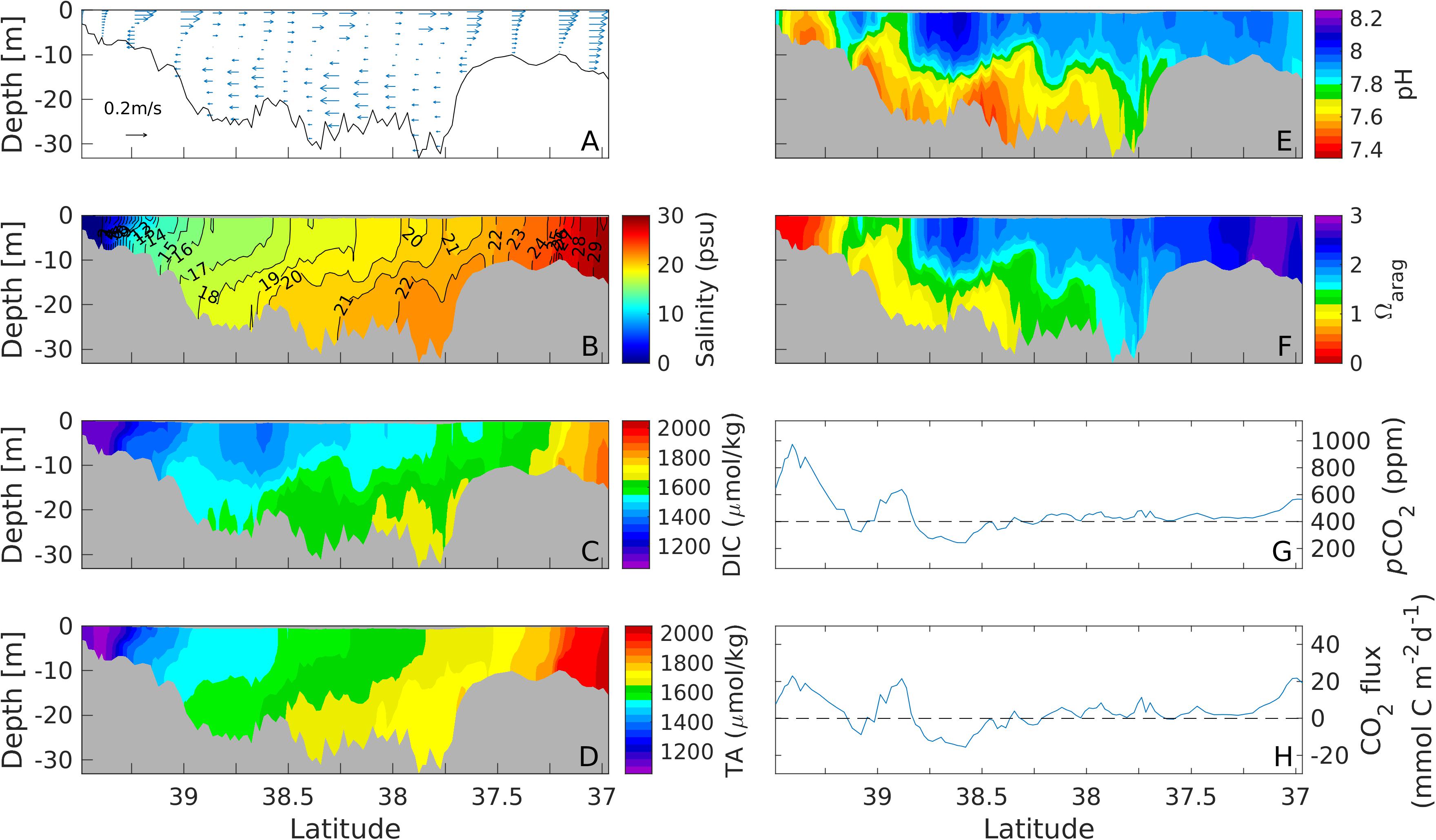
Figure 7. Along channel distributions of subtidal current (A), salinity (B), DIC (C), TA (D), pH (E), Ω_arag (F), surface pCO₂ (G) and air-sea CO₂ flux (H) during a down-estuary wind event on 22–25 September, 2013.

In the cross-channel section, the down-estuary winds drove a counter-clockwise lateral circulation, with upwelling on the eastern shore and downwelling on the western shore (Figure 8A). Isohalines were tilted upward, with water in the intermediate depths (∼15 m) uplifted toward the steep eastern shoal, with the isohalines outcropping at a distance from the coastline (Figure 8B). Due to the steep bathymetry on the eastern flank of the deep channel, the upwelling was the most intense slightly away from the shore rather than at the coastline. Both DIC and TA were uplifted upward over the eastern shoal, with the highest values at about 1 km from the shoreline, as shown in the doming of DIC and TA isohalines (Figures 8C,D). In the surface layer down to 15 m depth, pH developed a strong lateral gradient, where pH reached a low value of 7.6–7.7 on the flank of the eastern shoal (5–10 m depth) and a high value of 8.0–8.1 on the western shoal (Figure 8E). The ventilation of high DIC water at 1 km off the eastern shoreline caused the surface water pCO₂ there to exceed the atmospheric value. The lateral distribution of air-sea CO₂ flux showed ingassing up to 15 mmol C m^–2 d^–1 on the western shoal and outgassing of up to 7 mmol C m^–2 d^–1 on the eastern shoal (Figure 8F).

FIGURE 8

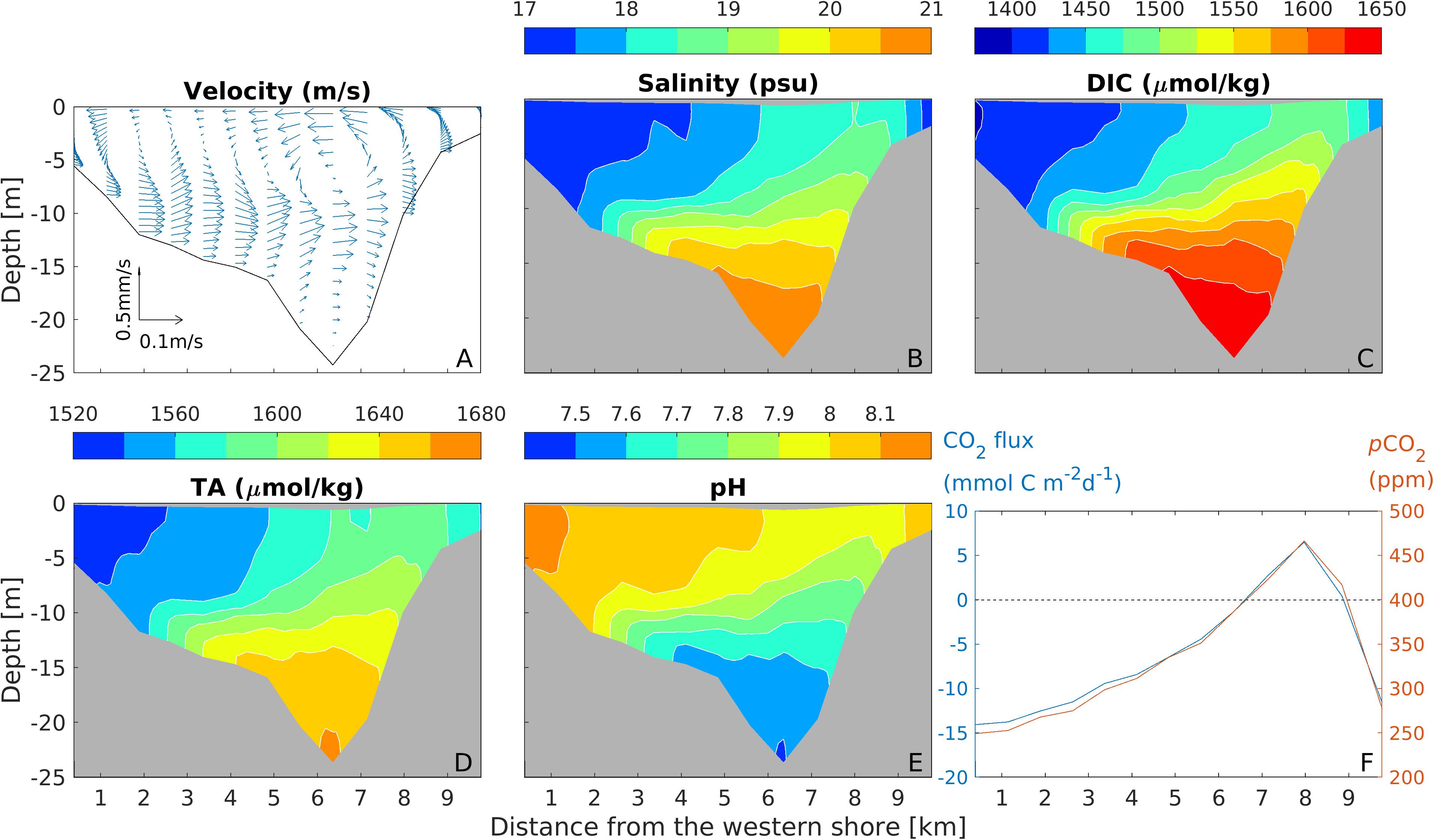
Figure 8. Distributions of lateral-vertical velocity vector (A), salinity (B), DIC (C), TA (D), pH (E), and surface pCO₂ (red) and air-sea CO₂ (blue) (F) at the mid-bay section during the down-estuary wind event.

Summary of Wind Effects

We have so far focused on the detailed analyses of two wind events. To summarize the overall effects of wind on the carbonate system, we investigated a number of weather events that moved across Chesapeake Bay during 2013. This analysis captured how the carbonate system evolved in different seasons due to changing seasonal prevailing wind directions and seasonal evolution of CO₂ uptake and respiration. Two regime diagrams were constructed to identify general relationships between winds and variations in pH, DIC and other carbonate parameters.

First we investigated wind-driven temporal changes in pH. At the three stations in the mid-Bay cross-section (the cross-section marked in Figure 1A and the three stations in this section marked in Figure 4D), the time series of surface and bottom water pH were filtered to remove tidal fluctuations and the pH change from the beginning (pH_begin) to the end (pH_end) of a wind event was calculated:

$$\mathrm{\delta }pH=p{H}_{end}-p{H}_{begin}.(1)$$

We also calculated similar quantity for the aragonite saturation state:

$$\mathrm{\delta }\text{Ω}{}_{arag}=\text{Ω}{}_{arag{}_{end}}-\text{Ω}{}_{arag{}_{begin}}(2)$$

where Ω_aragbegin and Ω_aragend are the values of Ω_arag the beginning and end of each wind event. The wind impulse, defined as

$$I_{wind}=\underset{begin}{\overset{end}{\int }}{\mathrm{\tau }}_{x}dt(3)$$

is an integrated measure of wind effects over a wind event and provides a good descriptor of the lateral upwelling effect. Here τ_x is the along-channel wind stress at a mid-Bay location and the integration is over the entire duration of a wind event. Figures 9A,C,D,F show that δpH and δΩ_arag at the two shallow shoals were approximately linearly proportional to I_wind, and that there was additional variability beyond that explained byI_wind. With δpH reaching up to ±0.3, pH fluctuated over a wide range during a wind event. Changes in Ω_arag were also large, reaching ±1.0. Under the down-estuary winds, δpHandδΩ_arag were positive (increased over time) on the western shoal but negative (decreased) on the eastern shoal. Under the up-estuary winds, δpH and δΩ_arag were negative (decreased over time) on the western shoal but positive (increased) on the eastern shoal. They varied out of phase because the lateral upwelling affected the two shoals in opposite ways. In contrast, δpH and δΩ_arag in the bottom water of the deep channel showed small changes, indicating that neither the direct wind mixing nor the lateral upwelling had much effect there (Figures 9B,E). δpH in the surface water of the deep channel showed much larger changes over each wind event and was mostly negative, indicating wind mixing injected lower pH subsurface water upward and reduced surface pH. In some cases, it became positive, suggesting that horizontal advection and straining may have brought high pH water to the mid-Bay section. δΩ_arag in the surface water of the deep channel showed changes compatible to δpH there (Figure 9E). With the exception of a few wind events, δpH and δΩ_arag in the deep channel showed much smaller fluctuations than those on the shallow shoals.

FIGURE 9

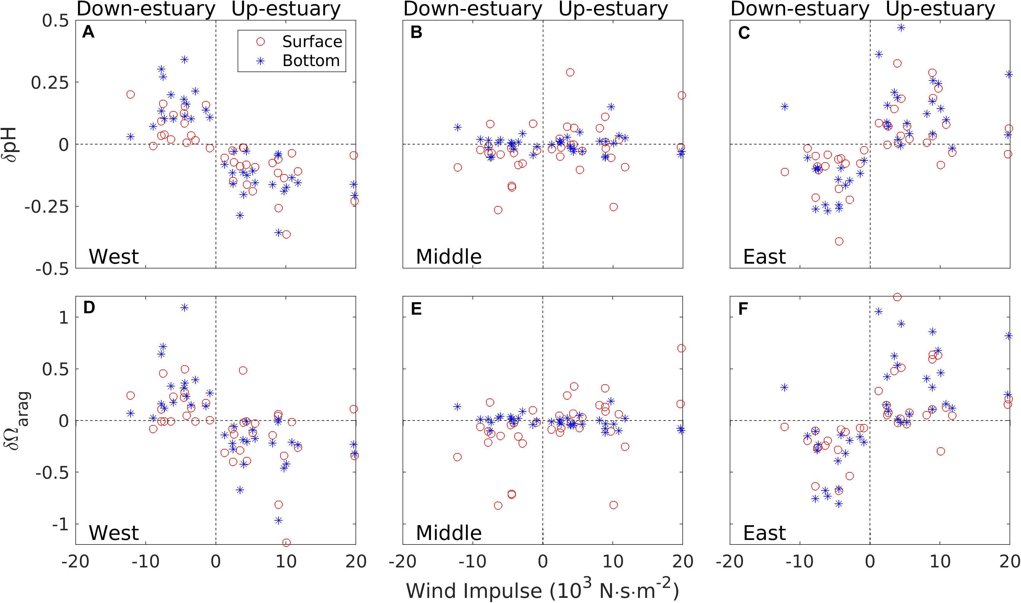
Figure 9. Summary of wind effects on the temporal variations in pH/aragonite saturation state Ω_arag at the western shoal location (A,D), the center channel (B,E), and the eastern shoal location (C,F): red open circles for surface pH/ Ω_arag and blue stars for bottom pH/ Ω_arag.

The lateral differences Δ_yDIC, Δ_ypH, and Δ_ypCO₂ were calculated as the DIC, pH and pCO₂ differences between the eastern and western flanks of the estuarine channel (each covering ∼1/3 of the cross-sectional area), averaged over each wind event. Instead of looking at one cross-channel section, we averaged Δ_yDIC and Δ_ypH over the mid-Bay (marked as the light blue area in Figure 1B) and over the entire main stem of the Bay (all shaded areas in Figure 1B). Figure 10A shows how Δ_yDIC averaged over the mid-Bay varied with I_w. Δ_yDICwas generally negative under the up-estuary winds (positive I_w) and positive under the down-estuary winds (negative I_w). This simply said that DIC was higher on the western shoal than on the eastern shoal under the up-estuary winds. The reverse was true under the down-estuary winds: DIC was higher on the eastern shoal than on the western shoal. Despite the scatter in the plot, Δ_yDIC generally increased with I_w. The stronger the wind speed or the longer the wind duration or both, the stronger the lateral gradient in DIC. There was a bias toward the upper right corner because of the downward tilt of isohalines and DIC-isolines due to the geostrophic balance (see Figure 4). Δ_yDIC can reach ±100μmol/kg. Because the lateral asymmetry was weaker in the narrow upper Bay and shallow lower Bay, ΔDIC over the entire Bay was smaller. Due to the geostrophic control in the lower Bay, Δ_yDIC was biased toward the positive value even under many up-estuary wind events (Figure 10D). The overall wind effects on the lateral asymmetry in the entire Bay were not as strong as in the mid-Bay.

FIGURE 10

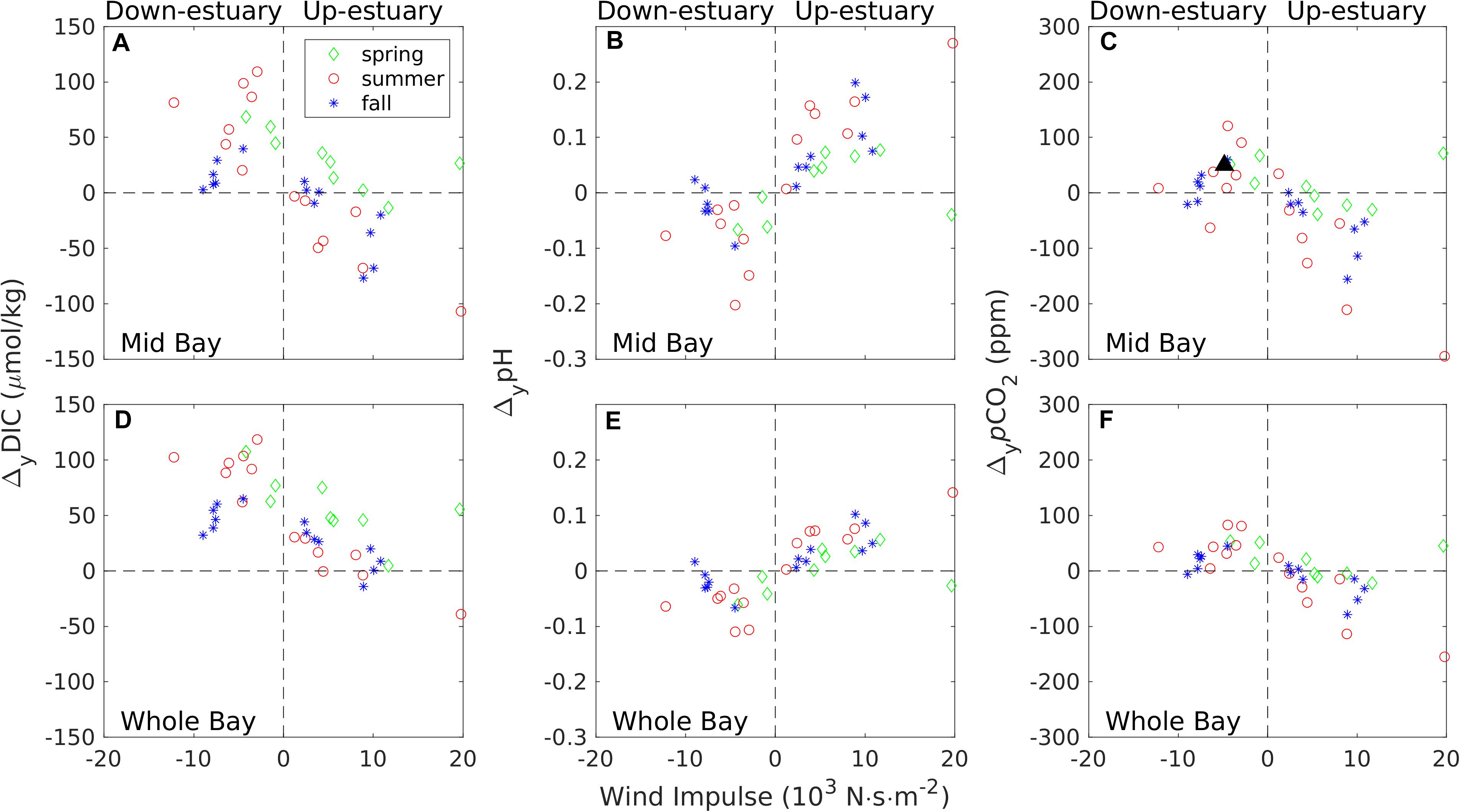
Figure 10. Summary of wind effects on the lateral asymmetry in estuarine carbonate system. Time averaged lateral difference (eastern one third-minus western one third) in DIC (A,D), pH (B,E), and pCO₂ (C,F) in the mid-Bay region (top panel) or over the entire Bay (bottom panel): spring (March–May, green diamonds), summer (June–August, red circles), fall (September–November, blue stars). The black triangle in (C) denoted the observational data from Huang et al. (2019).

pH averaged over the top 5 m in the water column also displayed the lateral asymmetry that extended to all seasons and all wind events (Figures 10B,E). In the mid-Bay, Δ_ypH > 0 for I_w > 0 and Δ_ypH < 0 for I_w < 0 (Figure 10B). Notwithstanding the scatters, ΔpH appears to be a linear function of I_w for I_w > 0. Therefore, pH was lower on the western shoal than on the eastern shoal under the up-estuary winds and this lateral difference Δ_ypH increased with the wind impulse. Under the down-estuary winds, the reverse asymmetry was true: pH was lower on the eastern shoal than on the western shoal. At I_w < 0 the magnitude of Δ_ypH was generally less than 0.1 (except two events) whereas Δ_ypH could reach 0.2 at I_w > 0. This asymmetry in Δ_ypH is related to the asymmetric response to wind direction: the lateral circulation strength and lateral upwelling are weaker under the down-estuary winds than under the-up-estuary winds (Li and Li, 2012; Xie et al., 2017). When averaged over the entire Bay, Δ_ypH versus I_w showed surprisingly tight relationship as seen in the mid-Bay (Figure 10E). The magnitude was smaller, down to ±0.1, as opposed to ±0.2 in the mid-Bay.

The lateral upwelling also generated pCO₂ variations in the lateral direction (Figures 10C,F). Under the up-estuary winds, pCO₂ on the western shoal was larger than that on the eastern shoal, i.e., Δ_ypCO₂ < 0 and its magnitude increased with the wind impulse. Under the down-estuary winds, the reverse was generally true, with Δ_ypCO₂ > 0. Huang et al. (2019) observed Δ_ypCO₂ = 50ppm during a down-estuary wind event with the maximum wind speed of 7 m/s and wind impulse of 4.84×10³Nsm⁻². The observed data fit well with the scatter plot in Figure 10C, indicating a general agreement between the model-predicted and observed pCO₂ lateral differences. The numerical model allowed us to explore a wide range of wind forcing conditions, and Figures 10C,F showed that winds can generate lateral pCO₂ differences in the range of ± 200ppm in the mid-Bay and in the range of ± 100ppm when averaged over the entire estuary.

Effects of Upwelling on Nearshore Habitats

Most of the current and historic mainstem eastern oyster (Crassostrea virginica) beds in Maryland are located on the shallow shoals in the mid-Bay between 37.9 and 39.1°N, as shown in Figure 11A (Smith, 1997). Wind-driven lateral upwelling could expose these oysters to episodic acidic conditions, particularly during the summer months when pH and Ω_arag reach seasonal minima in bottom waters, and exposure of the eastern oyster to low pH and under-saturated waters could have potentially negative consequences for growth and calcification (Waldbusser and Salisbury, 2014; Waldbusser et al., 2015). Under the weak winds, the aragonite saturation state Ω_arag on a narrow strip along the western shoal and a broader region on the eastern shoal exceeded 1, suggesting limited influence of deep-channel bottom water on most of the historic oyster beds (Figure 11B). In contrast to the shallow shoals, bottom water was highly undersaturated, with Ω_arag around 0.5. Under the up-estuary winds, Ω_arag fell below 1 almost everywhere on the western shoal, with the minimum value dropping down to 0.6 (Figure 11C). On the other hand, Ω_arag increased on the eastern shoal, suggesting that dissolution-favorable conditions would not occur. Under the down-estuary winds, the most intense upwelling occurred channel-ward of the eastern coastline (Figure 8C) such that Ω_arag remained above 1 over the shallowest regions on the eastern shoal (Figure 11D). During the same down-estuary winds, Ω_arag increased to 2–3 on the fringe along the western coastline.

FIGURE 11

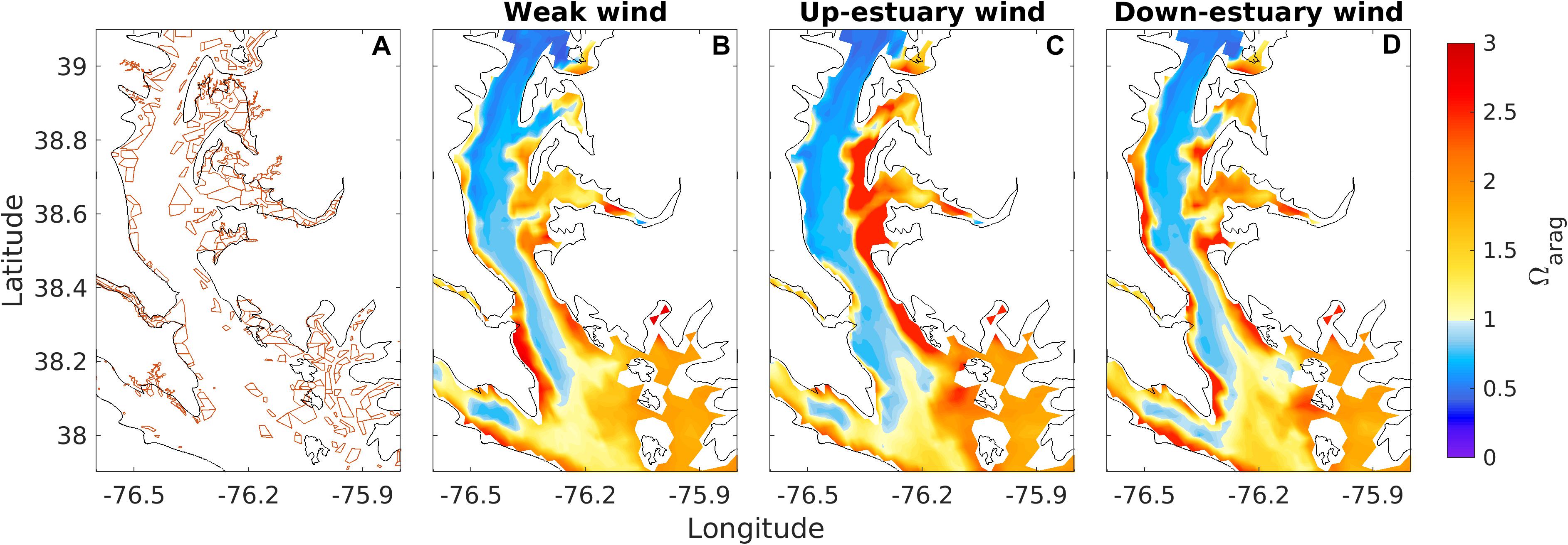
Figure 11. Distribution of Maryland’s oyster bed in Chesapeake Bay (A) and bottom water aragonite saturation state Ω_arag in the oyster habitat under weak (B), up-estuary (C), and down-estuary (D) winds during August, 2003.

The duration of exposure to undersaturated conditions is an important factor for potentially negative growth and calcification effects on bivalves. We calculated the time which the bottom water Ω_arag < 1 persisted during each wind event, using the two shallow-shoal locations in the mid-Bay (Figure 4B) as examples. During the spring and summer, the bottom water on the western shoal was exposed to undersaturated conditions for a period ranging from 5 to 60 h (Figure 12A). The bottom water was rarely exposed to Ω_arag < 1 during the fall. Since the location on the eastern shoal is further inshore than the most-intense upwelling region, the bottom water there was exposed to fewer wind events with an extended period of undersaturated conditions (Figure 12B).

FIGURE 12

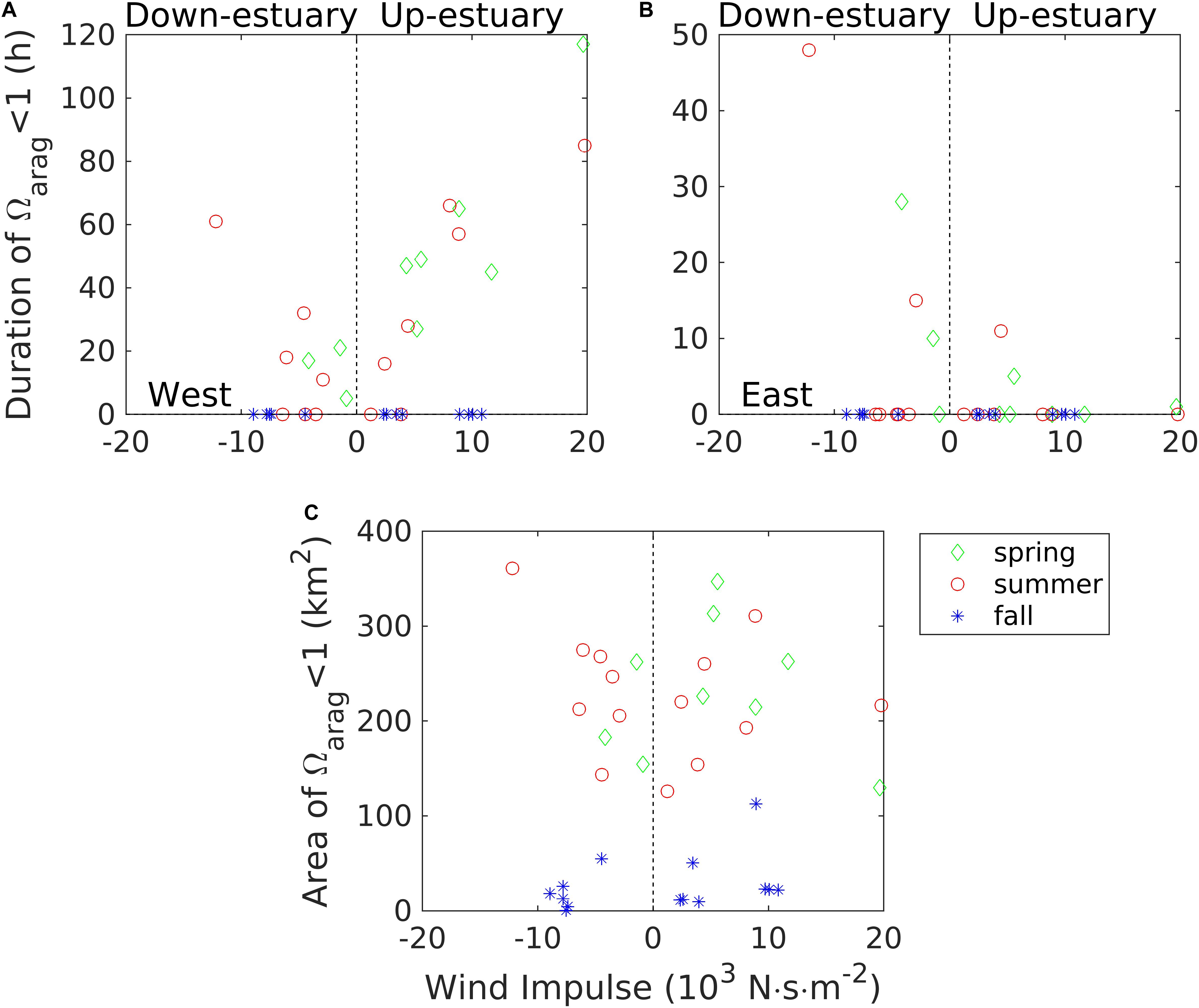
Figure 12. Duration of aragonite saturation state Ω_arag < 1 in bottom waters at the western shoal (A) and the eastern shoal (B) locations in the mid-Bay cross-section. (C) The size of mainstem oyster beds in Maryland affected by under-saturated water (Ω_arag < 1) during wind events. Green diamonds for spring, red circles for summer, and blue stars for fall.

To examine the regional spatial impacts of wind-driven lateral upwelling, we calculated the size A_oyster of the sea bed areas in the mid-Bay during each wind event. We computed the area between 37.9 and 39.1°N where depth <8 m and Ω_arag < 1 for three different seasons (spring, summer, and fall). A_oyster in spring and summer was a U-shaped function of the wind impulse, implying that more areas of the oyster beds were exposed to undersaturated conditions at higher wind speed or longer wind duration on both the eastern and western shoals (Figure 12C). About 100–300 km² of this area could be exposed to Ω_arag < 1 during the spring and summer seasons, which is about 25–75% of the total oyster bed area. During the fall, pH and Ω_arag were higher such that only a small area (generally less than 50 km²) was affected.

Discussion

This study showed that winds can drive pH fluctuations of up to 0.3 in Chesapeake Bay over a period of a few days. These pH fluctuations are comparable to or larger than the long-term pH (0.1–0.2) decline that has been observed in Chesapeake Bay over the past three decades (Waldbusser et al., 2011; Shen et al., 2020). This adds to a growing body of evidence for large pH variability in coastal and estuarine systems (Carstensen and Duarte, 2019). Hofmann et al. (2011) analyzed high resolution time series of upper ocean pH obtained using autonomous sensors, over a variety of systems from polar to tropical regions. In the four coastal and estuarine sites on the United States West Coast, the standard deviations from the monthly mean pH ranged from 0.07 to 0.13, of a similar magnitude as found here. In a seagrass habitat of Hat Island in Puget Sound, Pacellaa et al. (2018) observed the mean diel range of pH of 0.39, with a maximum observed diel range of 0.74. The diel photosynthesis/respiration cycle was a major driver of this large pH variability, but tidal advection of metabolically altered parcels and wind-driven mixing events also played important roles. Similarly, measurements in a macrophyte meadow of the Baltic Sea showed that pH can vary from 8.22 ± 0.1 in August to 7.83 ± 0.4 in September (Saderne et al., 2013). Daily variations of pCO₂ due to photosynthesis and respiration were a major cause for this pH variability, but local upwelling of elevated pCO₂ water masses with offshore winds drove the variations at a time scale of days to weeks. Thus, winds and local productivity interact to drive high frequency variations in estuaries.

Winds may affect the carbonate system in an estuary or a coastal ocean in a number of ways. Depending on the air-sea difference in pCO₂, winds can drive a large efflux or influx of CO₂ and change surface water DIC and pH (Huang et al., 2015). Wind-driven mixing can mix high DIC, high CO₂ and low pH bottom waters to the surface layer and reduce surface pH (Cai et al., 2017; Moore-Maley et al., 2018). Wind-driven upwelling can deliver acidic and carbonate undersaturated waters onto continental shelves (Feely et al., 2008; Hauri et al., 2009). Our analysis showed that wind-driven lateral upwelling could cause larger pH fluctuations on shallow shoals than those caused by direct wind mixing in Chesapeake Bay (Figures 2, 9). This upwelling mechanism is similar to that in large-scale coastal upwelling systems (e.g., Pacific coast of North America), even though winds are weaker and more variable. The upwelling velocity in Chesapeake Bay is <0.5 mm s^–1 (Figures 6A, 8A), only a fraction of the typical upwelling velocity (2 mm s^–1) found in large coastal upwelling systems (Johnson, 1977). However, it can still deliver deep acidic water to the shallow shoals because water depths in the estuary are only a few to tens of meters. For a synoptic weather event with a mean wind speed of 5 m s^–1 and a duration of 2 days, the wind impulse is 8.6×10³Nsm⁻², well within the range reported in Figures 9, 12 and typically observed in estuarine and coastal regions. Our result for the dominance of upwelling over mixing in driving pH fluctuations is consistent with a related hypoxia modeling study in which Scully (2010) showed that wind-driven lateral upwelling and ventilation of deep hypoxic water onto shallow shoals are more important than wind mixing in supplying dissolved oxygen to the bottom water. This is probably more so for CO₂ than for O₂ as the air-sea gas exchange flux is generally much smaller for CO₂ than for O₂ (Jiang et al., 2019).

The wind-driven lateral upwelling generated large lateral differences in DIC. The relationship between Δ_yDIC and I_w holds better in the mid-Bay than in the entire estuary (Figure 10), as the wind-driven lateral circulation is strongest in the wide mid-Bay that features a deep channel and broad shoals. Moreover, the vertical gradient in DIC and pH there is strongest due to DIC consumption in the surface layer and DIC production in the bottom layer, such that upwelling of acidic deep water has the largest effects on the shallow shoals. In comparison, the lateral circulation is much weaker in the shallow and narrow upper Bay. Strong lateral circulation can develop in the lower Bay (Xie and Li, 2018), but the vertical DIC gradient is much smaller there than that in the mid-Bay such that the upwelling does not induce large changes in surface water DIC. When integrated over the entire Bay, the relationship between Δ_yDIC and I_w (and the lateral DIC asymmetry) is less robust than in the mid-Bay. Δ_yDIC is approximately a linear function of I_w under the up-estuary winds but displays more scatters under the down-estuary winds. In a numerical modeling study, Li and Li (2012) showed that at the same wind speed the lateral circulation strength is 2–3 times stronger under the up-estuary winds than under the down-estuary winds. Using velocity measurements collected at a cross-channel array of AD, Xie et al. (2017) observed that the lateral circulation on the western part of the estuarine channel was weakened considerably due to the effect of baroclinic forcing under the down-estuary winds. Therefore, the larger scatter in Δ_yDIC versus I_w under the down-estuary winds is likely caused by the weaker lateral circulation. We note that the scatter seen in Figure 10 are comparable to that in the plot for the lateral circulation strength reported in Xie et al. (2017) because the wind-driven lateral circulation is not only determined by the wind speed but also affected by river flows, offshore salinity and lateral baroclinic forcing.

Unlike DIC and pH, the air-sea CO₂ flux does not demonstrate a simple dependence on the wind speed/direction or wind impulse (Supplementary Figures S3–S5). As Shen et al. (2019a) and Chen et al. (2020) showed recently, Chesapeake Bay is releasing CO₂ into the atmosphere in the upper Bay, absorbing it in the mid-Bay and near the equilibrium condition in the lower Bay. While wind-driven mixing and straining/ventilation can result in locally enhanced CO₂ flux (Figures 5H, 7H) and lateral upwelling can generate cross-channel gradients in CO₂ flux (Figures 6F, 8F), the overall wind effects on the air-sea CO₂ exchange over the entire estuary cannot be easily quantified. As discussed earlier, wind effects are most pronounced in the deep hypoxic mid-Bay where respiration of organic matter creates strong vertical gradients in DIC. Typically, the mid-Bay is a net sink of CO₂ due to strong phytoplankton production in the surface euphotic layer and the surface water pCO₂ is in the range of 200–300 ppm which is less than the atmospheric pCO₂ of 400 ppm. Wind-induced mixing and ventilation in the deep channel raises surface water pCO₂, but the net wind effect on the CO₂ flux depended on whether the surface water pCO₂ remains below or rises above the atmospheric value. If the surface water pCO₂ < 400 ppm, the winds would pump more CO₂ into the estuary and this influx/sink increases with the wind speed. For example, the up-estuary wind event U17 caused a peak CO₂ influx of −65.3 × 10⁶ mol C d^–1 over the mid-Bay and −61.4 × 10⁶ mol C d^–1 over the entire estuary (Supplementary Figure S5). If the surface water pCO₂ > 400 ppm, however, the winds will release CO₂ into the atmosphere, turning Chesapeake Bay from a weak CO₂ sink to a source. For example, during the down-estuary wind event D8, the surface water pCO₂ increased to 672.9 ppm, such that there was a peak CO₂ efflux of 133.7 × 10⁶ mol C d^–1 over the mid-Bay and 340.6 × 10⁶ mol C d^–1 over the entire estuary (Supplementary Figure S4). Similarly, the wind-driven upwelling changes the lateral distribution of pCO₂, but its net effect on the CO₂ flux depends on the balance between the excess and deficits in the CO₂ flux at the two shallow shoals flanking the deep channel. Overall, the complicated non-linear dependence of CO₂ flux on the wind speed and strong spatial variability make it difficult to identify a simple relationship between the CO₂ flux and wind forcing in this estuary. Although numerical model estimates of air-sea@ CO₂ flux can help overcome challenges in making similar estimates from limited and error-prone observations (Herrmann et al., 2020), assigning causation to these changes under dynamic physical forcing is difficult even with model simulations.

Lateral upwelling of oxygen poor, acidic water onto otherwise oxic and high-pH shallow shoals in Chesapeake Bay has been documented in previous studies (e.g., Malone et al., 1986; Sanford et al., 1990; Scully, 2010; Huang et al., 2019), but its potential impact on oyster beds has not been specifically investigated in this estuary. In contrast, upwelling of acidic waters and it impacts on bivalves have been clearly documented along the Pacific coast of North America (e.g., Feely et al., 2008). We found that southerly or southeasterly (up-estuary winds) during the summer led to upwelling of corrosive water onto the western shoal where oyster beds have previously been identified, and that the duration of these events in 2013 led to 1–3 day periods with water with Ω_arag < 1. Although Waldbusser et al. (2011) documented reduced biocalcification in juvenile eastern oysters as W_calcite declined, they also found that net calcification could occur under moderately corrosive conditions (W_calcite ∼0.7–1). However, net dissolution in the eastern oyster occurred below Ω_arag = 0.6, and studies focused on other juvenile bivalves found reduced growth and mortality under comparable conditions (e.g., Green et al., 2009). The relatively brief duration of upwelling events in Chesapeake Bay may not be sufficiently chronic to induce reduced growth, calcification, or other physiological consequences (Talmage and Gobler, 2010; Keppel et al., 2016), but repeated exposures to these conditions may eventually be detrimental.

To account for accumulated acidification stress on larval bivalves, Gimenez et al. (2018) recently defined a new metric: ocean acidification stress index for shellfish (OASIS):

$$\begin{array}{cc}OASIS=\underset{fertilization}{\overset{settlement}{\int }}\left[({\text{Ω}}_{thrsh}-\text{Ω}{}_{arag})\frac{1}{1+D_{pft}}\right]dt,\hfill & \\ if({\text{Ω}}_{thrsh}-\text{Ω}{}_{arag})>0\hfill & \end{array}$$

where Ω_thrsh is the selected acidification stress threshold and D_pft is the day(s) post-fertilization (spawning day = 0). OASIS has the unit of Ω min day^–1 and provides a measure of accumulated stress by integrating only the area of the Ω_arag time series that falls below the designated threshold over the entire larval period, from fertilization to metamorphosis. Although the experimental study by Gimenez et al. (2018) focused on the Pacific oyster, it is instructive to calculate OASIS using the model results presented in Figure 12. We adopted the same conservative threshold of Ω_thrsh = 1.5. Figure 13 shows how the OASIS index at the two shallow shoal locations in the mid-Bay cross section varies with the wind impulse, and the OASIS response largely mirrors that of low Ω_arag duration and area (Figure 12). OASIS was small during the fall, indicating limited acidification stress on the oyster larvae, but fall conditions may not be as important because oysters typically spawn between June and August (Kennedy, 1996). However, OASIS increased rapidly with I_w during the spring and summer, a time when eastern oyster gametes are beginning to ripen and spawning occurs, respectively (Kennedy, 1996). At the western shoal location, OASIS reached 500–1500 Ω min day^–1 in the summer, which could cause a significant reduction in oyster larval survival rate (Gimenez et al., 2018) at a time when spawning is actively occurring. Furthermore, the interaction of exposures to both corrosive and hypoxic waters during these upwelling events may also have synergistic consequences for organisms (e.g., Miller et al., 2016). Clearly, there remains much to be learned concerning the potential impacts of upwelling events on biological communities, and the model simulations presented here provide a quantitative tool for prediction of the severity, duration, and frequency of such events in response to seasonally varying winds.

FIGURE 13

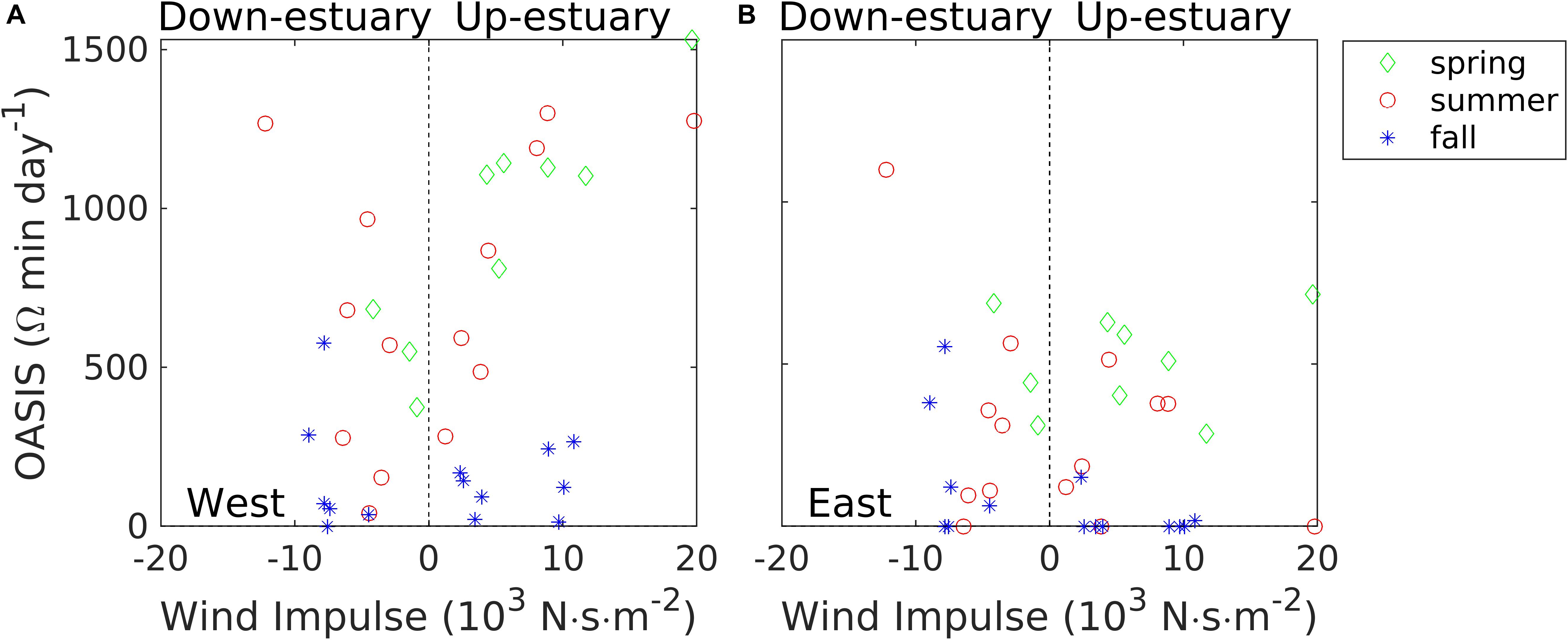
Figure 13. OASIS (Ocean Acidification Stress Index for Shellfish) in bottom waters at the western shoal (A) and the eastern shoal (B) locations in the mid-Bay cross-section. Green diamonds for spring, red circles for summer, and blue stars for fall.

In summary, we used a numerical model to quantify the impacts of along-axis wind stress on the lateral dynamics of the carbonate system in Chesapeake Bay, a large estuary with moderate tides. Although the upwelling of corrosive and acidified water in response to wind is widely recognized in coastal oceans, this study provides the first mechanistic explanation that wind-driven lateral upwelling can deliver acidified deep water to shallow shoals in estuaries, producing large temporal pH and Ω_arag fluctuations. Fluctuations in pH could reach ±0.3, depending on the combined effect of wind speed and wind duration as represented by the wind impulse. Changes in Ω_arag were also large, reaching ±1.0. Regime diagrams are constructed to summarize the effects of wind events on temporal pH and Ω_arag fluctuations and the lateral gradients in DIC, pH, and pCO₂ in the estuary. Given the potential for expanded low-pH bottom waters under warming-enhanced respiration, elevated riverine inputs, and increasing atmospheric CO₂, Chesapeake Bay may be more vulnerable to more frequent or intense future upwelling events. Future studies of estuarine acidification need to consider the intensity and control of these events, as well as the effects of these physically driven pH fluctuations on organisms’ physiological response.

Data Availability Statement

Publicly available datasets were analyzed in this study. This data can be found here: https://zenodo.org/record/3964478#.XyBNRxIh2Uk.

Author Contributions

ML, W-JC, and JT conceived and designed the numerical experiments. RL conducted the numerical model simulations. CS assisted in the model configurations. RL and ML analyzed the model results. ML wrote the manuscript with editorial contributions from W-JC and JT. All authors contributed to the article and approved the submitted version.

Funding

We are grateful to the NOAA Ocean Acidification Program (NOAA-OAP; Awards NA15NOS4780184 and NA18NOS4780179) for the financial support.

Conflict of Interest

The authors declare that the research was conducted in the absence of any commercial or financial relationships that could be construed as a potential conflict of interest.

Acknowledgments

We thank the two reviewers for helpful comments and George Waldbusser for brining our attention to the OASIS calculations. This is UMCES contribution number 5923.

Supplementary Material

The Supplementary Material for this article can be found online at: https://www.frontiersin.org/articles/10.3389/fmars.2020.588465/full#supplementary-material

Footnotes

1. ^ https://www.chesapeakebay.net/what/data

References

Bakker, D. C. E., Pfeil, B., Landa, C. S., Metzl, N., O’Brien, K. M., and Olsen, A., et al. (2016). A multi-decade record of high-quality fCO₂ data in version 3 of the Surface Ocean CO₂ Atlas (SOCAT). Earth Syst. Sci. Data 8, 383–413. doi: 10.5194/essd-8-383-2016

CrossRef Full Text | Google Scholar

Baumann, H., and Smith, E. M. (2018). Quantifying metabolically driven pH and oxygen fluctuations in US nearshore habitats at diel to interannual time scales. Estuar. Coast. 41, 1102–1117. doi: 10.1007/s12237-017-0321-3

CrossRef Full Text | Google Scholar

Baumann, H., Wallace, R. B., Tagliaferri, T., and Gobler, C. J. (2015). Large natural pH, CO2 and O2 fluctuations in a temperate tidal salt marsh on diel, seasonal, and interannual time scales. Estuar. Coast. 38, 220–231. doi: 10.1007/s12237-014-9800-y

CrossRef Full Text | Google Scholar

Borges, A. V., and Gypens, N. (2010). Carbonate chemistry in the coastal zone responds more strongly to eutrophication than to ocean acidification. Limnol. Oceanogr. 55, 346–353. doi: 10.4319/lo.2010.55.1.0346

CrossRef Full Text | Google Scholar

Brady, D. C., Testa, J. M., Di Toro, D. M., Boynton, W. R., and Kemp, W. M. (2013). Sediment flux modeling: calibration and application for coastal systems. Estua. Coast. Shelf Sci. 117, 107–124. doi: 10.1016/j.ecss.2012.11.003

CrossRef Full Text | Google Scholar

Breitburg, D. L. (1992). Episodic hypoxia in Chesapeake Bay: interacting effects of recruitment, behavior, and physical disturbance. Ecol. Monogr. 62, 525–546. doi: 10.2307/2937315

CrossRef Full Text | Google Scholar

Brodeur, J. R., Chen, B., Zhong, J., Xu, Y., Hussain, N., Scaboo, K. M., et al. (2019). Chesapeake Bay inorganic carbon, spatial distribution and seasonal variability. Front. Mar. Sci. 6:99. doi: 10.3389/fmars.2019.00099

CrossRef Full Text | Google Scholar

Browne, D. R., and Fisher, C. W. (1988). Tide and Tidal Currents in the Chesapeake Bay. NOAA Technical Report NOS OMA 3 84. Washington, DC: NOAA.

Google Scholar

Cai, W., Hu, X., Huang, W., Murrell, M. C., Lehrter, J. C., Lohrenz, S. E., et al. (2011). Acidification of subsurface coastal waters enhanced by eutrophication. Nat. Geosci. 4, 766–770. doi: 10.1038/ngeo1297

CrossRef Full Text | Google Scholar

Cai, W., Huang, W., Luther, G. W., Pierrot, D., Li, M., Testa, J. M., et al. (2017). Redox reactions and weak buffering capacity lead to acidification in the Chesapeake Bay. Nat. Commun. 8:369.

Google Scholar

Cai, W.-J., Feely, R., Testa, J. M., Li, M., Evans, W., Alin, S., et al. (2021). Natural and anthropogenic drivers of acidification in large estuaries. Ann. Rev. Mar. Sci. [Epub ahead of print].

Google Scholar

Cai, W.-J., Hu, X., Huang, W.-J., Jiang, L.-Q., Wang, Y., Peng, T. H., et al. (2010). Alkalinity distribution in the western North Atlantic Ocean margins. J. Geophys. Res. Ocean 115:C08014. doi: 10.1029/2009JC005482

CrossRef Full Text | Google Scholar

Cai, W.-J., and Wang, Y. (1998). The chemistry, fluxes and sources of carbon dioxide in the estuarine waters of the Satilla and Altamaha Rivers, Georgia. Limnol. Oceanogr. 43, 657–668. doi: 10.4319/lo.1998.43.4.0657

CrossRef Full Text | Google Scholar

Cai, W.-J., Xu, Y.-Y., Feely, R. A., Wanninkhof, R., Jönsson, B., Alin, S., et al. (2020). Controls on surface water carbonate chemistry along North American ocean margins. Nat. Commun. 11:2691. doi: 10.1038/s41467-020-16530-z

PubMed Abstract | CrossRef Full Text | Google Scholar

Carstensen, J., and Duarte, C. M. (2019). Drivers of pH variability in coastal ecosystems. Environ. Sci. Technol. 53, 4020–4029. doi: 10.1021/acs.est.8b03655

PubMed Abstract | CrossRef Full Text | Google Scholar

Carter, H. H., and Pritchard, D. W. (1988). “Oceanography of Chesapeake Bay,” in Hydrodynamics of Estuaries: Dynamics of Partially-Mixed Estuaries, Vol. 1, ed. B. Kjerfe (Boca Raton, FL: CRC Press), 1–16.

Google Scholar

Chen, B., Cai, W.-J., Brodeur, J. R., Hussain, N., Testa, J. M., Ni, W., et al. (2020). Seasonal and spatial variability in surface pCO₂ and air-water CO₂ flux in the Chesapeake Bay. Limnol. Oceanogr. [Epub ahead of print]. doi: 10.1002/lno.11573

CrossRef Full Text | Google Scholar

Chen, S.-N., and Sanford, L. P. (2009). Axial wind effects on stratification and longitudinal salt transport in an idealized, partially mixed estuary. J. Phys. Oceanogr. 39, 1905–1920. doi: 10.1175/2009JPO4016.1

CrossRef Full Text | Google Scholar

Cheng, P., Li, M., and Li, Y. (2013). Generation of an estuarine sediment plume by a tropical storm. J. Geophys. Res. Oceans 118, 1–13. doi: 10.1029/2012JC008225

CrossRef Full Text | Google Scholar

Di Toro, D. M. (2001). Sediment Flux Modeling. New York, NY: Wiley-Interscience.

Google Scholar

Egbert, G. D., and Erofeeva, S. Y. (2002). Efficient inverse modeling of barotropic ocean tides. J. Atmos. Ocean Tech. 19, 183–204. doi: 10.1175/1520-0426(2002)019<0183:eimobo>2.0.co;2

CrossRef Full Text | Google Scholar

Eggleston, D. B., Bell, G. W., and Amavisca, A. D. (2005). Interactive effects of episodic hypoxia and cannibalism on juvenile blue crab mortality. J. Exp. Mar. Biol. Ecol. 325, 18–26. doi: 10.1016/j.jembe.2005.04.023

CrossRef Full Text | Google Scholar

Fairall, C. W., Bradley, E. F., Hare, J. E., Grachev, A. A., and Edson, J. B. (2003). Bulk parameterization of air–sea fluxes: updates and verification for the COARE algorithm. J. Clim. 16, 571–591. doi: 10.1175/1520-0442(2003)016<0571:bpoasf>2.0.co;2

CrossRef Full Text | Google Scholar

Feely, R. A., Alin, S. R., Newton, J., Sabine, C. L., Warner, M., Devol, A. H., et al. (2010). The combined effects of ocean acidification, mixing, and respiration on pH and carbonate saturation in an urbanized estuary. Estuar. Coast. Shelf Sci. 88, 442–449. doi: 10.1016/j.ecss.2010.05.004

CrossRef Full Text | Google Scholar

Feely, R. A., Sabine, C. L., Hernandez-Ayon, J. M., Ianson, D., and Hales, B. (2008). Evidence for upwelling of corrosive “acidified” water onto the continental shelf. Science 320, 1490–1492. doi: 10.1126/science.1155676

PubMed Abstract | CrossRef Full Text | Google Scholar

Filippino, K. C., Mulholland, M. R., and Bernhardt, P. W. (2011). Nitrogen uptake and primary productivity rates in themid-Atlantic bight (MAB). Estuar. Coast. Shelf Sci. 91, 13–23. doi: 10.1016/j.ecss.2010.10.001

CrossRef Full Text | Google Scholar

Friedman, J. R., Shadwick, E. H., Friedrichs, M. A. M., Najjar, R. G., De Meo, O. A., Da, F., et al. (2020). Seasonal variability of the CO₂ system in a large coastal plain estuary. J. Geophys. Res. Oceans 125:e2019JC015609. doi: 10.1029/2019JC015609

CrossRef Full Text | Google Scholar

Geyer, W. R., Woodruff, J. D., and Traykovski, P. (2001). Sediment transport and trapping in the Hudson River estuary. Estuar. Coasts 24, 670–679. doi: 10.2307/1352875

CrossRef Full Text | Google Scholar

Gimenez, I., Waldbusser, G. G., and Hales, B. (2018). Ocean acidification stress index for shellfish (OASIS): linking Pacific oyster larval survival and exposure to variable carbonate chemistry regimes. Elem. Sci. Anth. 6:51. doi: 10.1525/elementa.306

PubMed Abstract | CrossRef Full Text | Google Scholar

Goodrich, D. M., and Blumberg, A. F. (1991). The fortnightly mean circulation of Chesapeake Bay. Estuar. Coast. Shelf Sci. 32, 451–462. doi: 10.1016/0272-7714(91)90034-9

CrossRef Full Text | Google Scholar

Green, M. A., Waldbusser, G. G., Reilly, S. L., Emerson, K., and O’Donnell, S. (2009). Death by dissolution: sediment saturation state as a mortality factor for juvenile bivalves. Limnol. Oceanogr. 54, 1037–1047. doi: 10.4319/lo.2009.54.4.1037

CrossRef Full Text | Google Scholar

Haidvogel, D. B., Arango, H., Budgell, W. P., Cornuelle, B. D., Curchitser, E., Di Lorenzo, E., et al. (2008). Ocean forecasting in terrain-following coordinates: formulation and skill assessment of the regional ocean modeling system. J. Comput. Phys. 227, 3595–3624. doi: 10.1016/j.jcp.2007.06.016

CrossRef Full Text | Google Scholar

Hauri, C., Gruber, N., Plattner, G.-K., Alin, S., Feely, R. A., Hales, B., et al. (2009). Ocean acidification in the California current system. Oceanography 22, 60–71. doi: 10.5670/oceanog.2009.97

CrossRef Full Text | Google Scholar

Herrmann, M., Najjar, R. G., Da, F., Friedman, J. R., Friedrichs, M. A. M., Goldberger, S., et al. (2020). Challenges in quantifying air-water carbon dioxide flux using estuarine water quality data: case study for Chesapeake Bay. J. Geophys. Res. Oceans 125:e2019JC015610. doi: 10.1029/2019JC015610

PubMed Abstract | CrossRef Full Text | Google Scholar

Hofmann, G. E., Smith, J. E., Johnson, K. S., Send, U., Levin, L. A., Micheli, F., et al. (2011). High-frequency dynamics of ocean pH: a multi-ecosystem comparison. PLoS One 6:e28983. doi: 10.1371/journal.pone.0028983

PubMed Abstract | CrossRef Full Text | Google Scholar

Huang, W.-J., Cai, W.-J., Wang, Y., Lohrenz, S. E., and Murrell, M. C. (2015). The carbon dioxide system on the Mississippi River-dominated continental shelf in the northern Gulf of Mexico: 1. Distribution and air-sea CO₂ flux. J. Geophys. Res. Oceans 120, 1429–1445. doi: 10.1002/2014jc010498

PubMed Abstract | CrossRef Full Text | Google Scholar

Huang, W.-J., Cai, W.-J., Xie, X., and Li, M. (2019). Wind-driven lateral variations of partial pressure of carbon dioxide in a large estuary. J. Mar. Syst. 195, 67–73. doi: 10.1016/j.jmarsys.2019.03.002

CrossRef Full Text | Google Scholar

Isleib, R. P. E., Fitzpatrick, J. J., and Mueller, J. (2007). The development of a nitrogen control plan for a highly urbanized tidal embayment. Proc. Water Environ. Feder. 5, 296–320. doi: 10.2175/193864707786619152

CrossRef Full Text | Google Scholar

Jiang, Z.-P., Cai, W.-J., Chen, B., Wang, K., Han, C., Roberts, B. J., et al. (2019). Physical and biogeochemical controls on pH dynamics in the northern Gulf of Mexico during summer hypoxia. J. Geophys. Res. Oceans 124, 5979–5998. doi: 10.1029/2019JC015140

CrossRef Full Text | Google Scholar

Johnson, D. R. (1977). Determining vertical velocities during upwelling off the Oregon coast. Deep Sea Res. 24, 171–180. doi: 10.1016/0146-6291(77)90551-3

CrossRef Full Text | Google Scholar

Kennedy, V. S. (1996). “Biology of larvae and spat,” in The Eastern Oyster: Crassostrea Virginica, eds V. S. Kennedy, R. I. E. Newell, and A. F. Eble (Maryland: Maryland Sea Grant College, College Park), 371–421.

Google Scholar

Keppel, A. G., Breitburg, D. L., and Burrell, R. B. (2016). Effects of Co-varying diel-cycling hypoxia and pH on growth in the juvenile eastern oyster, Crassostrea virginica. PLoS One 11:e0161088. doi: 10.1371/journal.pone.0161088

PubMed Abstract | CrossRef Full Text | Google Scholar

Lacy, J. R., Stacey, M. T., Burau, J. R., and Monismith, S. G. (2003). Interaction of lateral baroclinic forcing and turbulence in an estuary. J. Geophys. Res. Oceans 108:3089. doi: 10.1029/2002JC001392

CrossRef Full Text | Google Scholar

Lerczak, J. A., and Geyer, W. R. (2004). Modeling the lateral circulation in straight stratified estuaries. J. Phys. Oceanogr. 34, 1410–1428. doi: 10.1175/1520-0485(2004)034<1410:mtlcis>2.0.co;2

CrossRef Full Text | Google Scholar

Lewis, E. R., and Wallace, D. W. R. (1998). CO2SYS-Program Developed for CO2 System Calculations. Tennessee: Carbon Dioxide Inf. Anal. Centre.

Google Scholar

Li, M., Lee, Y. J., Testa, J. M., Li, Y., Ni, W., Kemp, W. M., et al. (2016). What drives interannual variability of hypoxia in Chesapeake Bay: climate forcing versus nutrient loading? Geophys. Res. Lett. 43, 2127–2134. doi: 10.1002/2015GL067334

CrossRef Full Text | Google Scholar

Li, M., Zhong, L., and Boicourt, W. C. (2005). Simulations of Chesapeake Bay estuary: sensitivity to turbulence mixing parameterizations and comparison with observations. J. Geophys. Res. Oceans 110:C12004. doi: 10.1029/2004JC002585

CrossRef Full Text | Google Scholar

Li, M., Zhong, L., Boicourt, W. C., Zhang, S., and Zhang, D. (2006). Hurricane-induced storm surges, currents and destratification in a semi-enclosed bay. Geophys. Res. Lett. 33:L02604. doi: 10.1029/2005GL024992

CrossRef Full Text | Google Scholar

Li, Y., and Li, M. (2011). Effects of winds on stratification and circulation in a partially mixed estuary. J. Geophys. Res. Oceams 116:C12012. doi: 10.1029/2010JC006893

CrossRef Full Text | Google Scholar

Li, Y., and Li, M. (2012). Wind-driven lateral circulation in a stratified estuary and its effects on the along-channel flow. J. Geophys. Res. Oceams 117:C09005. doi: 10.1029/2011JC007829

CrossRef Full Text | Google Scholar

Li, Y., Li, M., and Kemp, W. M. (2015). A budget analysis of bottom-water dissolved oxygen in Chesapeake Bay. Estuar. Coast. 38, 2132–2148. doi: 10.1007/s12237-014-9928-9

CrossRef Full Text | Google Scholar

Loesch, H. (1960). Sporadic mass shoreward mgrations of demersal fish and crustaceans in Mobile Bay, Alabama. Ecology 41, 292–298. doi: 10.2307/1930218

CrossRef Full Text | Google Scholar

Malone, T. C., Kemp, W. M., Ducklow, H. W., Boynton, W. R., Tuttle, J. H., and Jonas, B. (1986). Lateral variation in the production and fate of phytoplankton in a partially stratified estuary. Mar. Ecol. Prog. Ser. 32, 149–160. doi: 10.3354/meps032149

CrossRef Full Text | Google Scholar

Miller, S. H., Breitburg, D. L., Burrell, R. B., and Keppel, A. G. (2016). Acidification increases sensitivity to hypoxia in important forage fishes. Mar. Ecol. Prog. Ser. 549, 1–8. doi: 10.3354/meps11695

CrossRef Full Text | Google Scholar

Moore-Maley, B. L., Ianson, D., and Allen, S. E. (2018). The sensitivity of estuarine aragonite saturation state and pH to the carbonate chemistry of a freshet-dominated river. Biogeosciences 15, 3743–3760. doi: 10.5194/bg-15-3743-2018

CrossRef Full Text | Google Scholar

Ni, W., Li, M., and Testa, J. M. (2020). Discerning effects of warming, sea level rise and nutrient management on long-term hypoxia trend in Chesapeake Bay. Sci. Total Environ. 737:139717. doi: 10.1016/j.scitotenv.2020.139717

CrossRef Full Text | Google Scholar

Pacellaa, S. R., Browna, C. A., Waldbusserb, G. G., Labiosac, R. G., and Halesb, B. (2018). Seagrass habitat metabolism increases short-term extremes and long-term offset of CO2 under future ocean acidification. PNAS 115, 2870–2875.

Google Scholar

Paerl, H. W., Crosswell, J. R., Van Dam, B., Hall, N. S., Rossignol, K. L., Osburn, C. L., et al. (2018). Two decades of tropical cyclone impacts on North Carolina’s estuarine carbon, nutrient and phytoplankton dynamics: implications for biogeochemical cycling and water quality in a stormier world. Biogeochemistry 141, 307–332. doi: 10.1007/s10533-018-0438-xvolV)

CrossRef Full Text | Google Scholar

Raymond, P. A., Bauer, J. E., and Cole, J. J. (2000). Atmospheric CO₂ evasion, dissolved inorganic carbon production, and net heterotrophy in the York River estuary. Limnol. Oceanogr. 45, 1707–1717. doi: 10.4319/lo.2000.45.8.1707

CrossRef Full Text | Google Scholar

Reynolds-Fleming, J. V., and Luettich, R. A. (2004). Wind-driven lateral variability in a partially mixed estuary. Estua. Coast. Shelf Sci. 60, 395–407. doi: 10.1016/j.ecss.2004.02.003

CrossRef Full Text | Google Scholar

Ribas-Ribas, M., Anfuso, E., Gomez-Parra, A., and Forja, J. M. (2013). Tidal and seasonal carbon and nutrient dynamics of the Guadalquivir estuary and the Bay of Cadiz (SW Iberian Peninsula). Biogeosciences 10, 4481–4491. doi: 10.5194/bg-10-4471-2013

CrossRef Full Text | Google Scholar

Saderne, V., Fietzek, P., and Herman, P. M. J. (2013). Extreme Variations of pCO2 and pH in a macrophyte meadow of the Baltic Sea in summer: evidence of the effect of photosynthesis and local upwelling. PLoS One 8:e62689. doi: 10.1371/journal.pone.0062689

PubMed Abstract | CrossRef Full Text | Google Scholar

Salisbury, J., Green, M., Hunt, C., and Campbell, J. (2008). Coastal acidification by rivers: a threat to shellfish? EOS Trans. AGU 89, 513–514. doi: 10.1029/2008eo500001

CrossRef Full Text | Google Scholar

Sanford, L. P., Sellner, K. G., and Breitburg, D. L. (1990). Covariability of dissolved-oxygen with physical processes in the summertime Chesapeake Bay. J. Mar. Res. 48, 567–590. doi: 10.1357/002224090784984713

CrossRef Full Text | Google Scholar

Scully, M. E. (2010). Wind modulation of dissolved oxygen in Chesapeake Bay. Estuar.Coast. 33, 1164–1175. doi: 10.1007/s12237-010-9319-9

CrossRef Full Text | Google Scholar

Scully, M. E., Geyer, W. R., and Lerczak, J. A. (2009). The Influence of lateral advection on the residual estuarine circulation: a numerical modeling study of the Hudson River estuary. J. Phys. Oceanogr. 39, 107–124. doi: 10.1175/2008jpo3952.1

CrossRef Full Text | Google Scholar

Shadwick, E. H., Friedrichs, M. A. M., Najjar, R. G., De Meo, O. A., Friedman, J. R., Da, F., et al. (2019). High frequency CO2 system variability over the winter-to-spring transition in a coastal plain estuary. J. Geophys. Res. Oceans 124, 7626–7642. doi: 10.1029/2019JC015246

CrossRef Full Text | Google Scholar

Shchepetkin, A. F., and McWilliams, J. C. (2005). The regional oceanic modeling system (ROMS): a split-explicit, free-surface, topography-following-coordinate oceanic model. Ocean Model. 9, 347–404. doi: 10.1016/j.ocemod.2004.08.002

CrossRef Full Text | Google Scholar

Shen, C., Testa, J. M., Li, M., and Cai, W.-J. (2020). Understanding anthropogenic impacts on pH and aragonite saturation state in Chesapeake Bay: insights from a 30-year model study. J. Geophys. Res. Biogeosci. 125:e2019JG005620. doi: 10.1029/2019JG005620

CrossRef Full Text | Google Scholar

Shen, C., Testa, J. M., Li, M., Cai, W.-J., Waldbusser, G. G., Ni, W., et al. (2019a). Controls on carbonate system dynamics in a coastal plain estuary: a modeling study. J. Geophys. Res. Biogeosci. 124, 61–78. doi: 10.1029/2018JG004802

CrossRef Full Text | Google Scholar

Shen, C., Testa, J. M., Ni, W., Cai, W.-J., Li, M., and Kemp, W. M. (2019b). Ecosystem metabolism and carbon balance in Chesapeake Bay: a 30-year analysis using a coupled hydrodynamic-biogeochemical model. J. Geophys. Res. Oceans 124, 6141–6153. doi: 10.1029/2019jc015296

CrossRef Full Text | Google Scholar

Smith, G. F. (1997). Maryland’s Historical Oyster Bottom: A Geographic Representation of the Traditional Named Oyster Bars. Oxford: Report of Fisheries Service, Maryland Department of Natural Resources and Cooperative Oxford Laboratory.

Google Scholar

Talmage, S. C., and Gobler, C. J. (2010). Effects of past, present, and future ocean carbon dioxide concentrations on the growth and survival of larval shellfish. PNAS 107, 17246–17251. doi: 10.1073/pnas.0913804107

PubMed Abstract | CrossRef Full Text | Google Scholar

Testa, J. M., Brady, D. C., Di Toro, D. M., Boynton, W. R., Cornwell, J. C., and Kemp, W. M. (2013). Sediment flux modeling: nitrogen, phosphorus and silica cycles. Estuar. Coast. Shelf Sci. 131, 245–263. doi: 10.1016/j.ecss.2013.06.014

CrossRef Full Text | Google Scholar

Testa, J. M., Li, Y., Lee, Y. J., Li, M., Brady, D. C., Di, D. M., et al. (2014). Quantifying the effects of nutrient loading on dissolved O2 cycling and hypoxia in Chesapeake Bay using a coupled hydrodynamic – biogeochemical model. J. Mar. Syst. 139, 139–158. doi: 10.1016/j.jmarsys.2014.05.018

CrossRef Full Text | Google Scholar

Testa, J. M., Li, Y., Lee, Y. J., Li, M., Brady, D. C., DiToro, D. M., et al. (2017). “Modeling physical and biogeochemical controls on dissolved oxygen in Chesapeake Bay: lessons learned from simple and complex approaches,” in Modeling Coastal Hypoxia - Numerical Simulations of Patterns, Controls and Effects of Dissolved Oxygen Dynamics, eds D. Justic, K. Rose, R. Hetland, and K. Fennel (Switzerland: Springer), 95–118. doi: 10.1007/978-3-319-54571-4_5

CrossRef Full Text | Google Scholar

Waldbusser, G. G., Hales, B., Langdon, C. J., Haley, B. A., Schrader, P., Brunner, E. L., et al. (2015). Saturation-state sensitivity of marine bivalve larvae to ocean acidification. Nat. Clim. Change 5, 273–280. doi: 10.1038/nclimate2479

CrossRef Full Text | Google Scholar

Waldbusser, G. G., and Salisbury, J. E. (2014). Ocean acidification in the coastal zone from an organism’s perspective: multiple system parameters, frequency domains, and habitats. Annu. Rev. Mar. Sci. 6, 221–247. doi: 10.1146/annurev-marine-121211-172238

PubMed Abstract | CrossRef Full Text | Google Scholar

Waldbusser, G. G., Voigt, E., Bergschneider, H., Green, M., and Newell, R. E. (2011). Biocalcification in the Eastern Oyster (Crassostrea virginica) in relation to long-term trends in Chesapeake Bay pH. Estua. Coast. 34, 221–231. doi: 10.1007/s12237-010-9307-0

CrossRef Full Text | Google Scholar

Wilson, R. E., Swanson, R. L., and Crowley, H. A. (2008). Perspectives on long-term variations in hypoxic conditions in western Long Island Sound. J. Geophys. Res. Oceans 113:C12011. doi: 10.1029/2007JC004693

CrossRef Full Text | Google Scholar

Xie, X., and Li, M. (2018). Effects of wind straining on estuarine stratification: a combined observational and modeling study. J. Geophys. Res. Oceans 123, 2363–2380. doi: 10.1002/2017JC013470

CrossRef Full Text | Google Scholar

Xie, X., Li, M., and Boicourt, W. C. (2017). Baroclinic effects on wind-driven lateral circulation in Chesapeake Bay. J. Phys. Oceanogr. 47, 433–445. doi: 10.1175/JPO-D-15-0233.1

CrossRef Full Text | Google Scholar

Zhong, L., and Li, M. (2006). Tidal energy fluxes and dissipation in the Chesapeake Bay. Cont. Shelf Res. 26, 752–770. doi: 10.1016/j.csr.2006.02.006

CrossRef Full Text | Google Scholar

Zhong, L., Li, M., and Foreman, M. G. (2008). Resonance and sea level variability in Chesapeake Bay. Cont. Shelf Res. 28, 2565–2573. doi: 10.1016/j.csr.2008.07.007

CrossRef Full Text | Google Scholar