Assessing the Potential Impact of Changes to the Argo and Moored Buoy Arrays in an Operational Ocean Analysis System

A series of observing system simulation experiments (OSSEs) have been carried out using the Met Office global Forecasting Ocean Assimilation Model (FOAM) to provide insights on the current and future design of the in situ observing network for ocean monitoring and forecasting. Synthetic observations are generated from a Nature Run (NR) that represents the true ocean state in the experiments. These observations are assimilated in FOAM and the results are compared to the NR to assess the impact of the observations, as well as assessing the effectiveness of the data assimilation system. The NR and FOAM based OSSEs have different resolutions and are driven by different surface forcing. The results show that assimilating observations equivalent to the current observing system allows the system to produce a realistic representation of the ocean state. Additional Argo profiles in some of the Western Boundary Current (WBC) regions and along the Equator improve the performance of FOAM by reducing the root mean square error (RMSE) against the Nature Run by ~10% for temperature and salinity fields in the upper ocean. Assimilating additional Deep Argo floats leads to ~20% RMSE reduction in basin scale regions and the reduction rate is up to 80% in the Labrador Sea below 2,500 m. An experiment withdrawing mooring profiles indicates the impact of moorings is localized and on average the analysis shows ~5% degradation without the mooring observations. The additional Argo profiles in the WBC regions and deep ocean also have impacts on the representation of the Ocean Heat Content (OHC) and the Atlantic Meridional Overturning Circulation (AMOC), with the deep Argo observations correcting the model drift in OHC below 2,000 m. The results highlight the necessity of a well-designed and coordinated in situ observing network globally, as well as requirements for future model and assimilation developments to achieve the best use of the additional in situ observations.

1. Introduction

Observations play an important role in initializing ocean models for various applications, from operational near-real time ocean forecasting to decadal predictions for climate studies (Fujii et al., 2019). While constellations of satellites altimeters and radiometers are mature, these provide only measurements of the near-surface ocean and integrated measures of the sub-surface. The global coverage of in situ ocean observations has improved significantly since 2000 with the deployment of the Argo array (Fu et al., 2018; Argo, 2020). The core Argo floats provide valuable information for the top 2,000 m of the world ocean, with almost no regular information for the ocean below 2,000 m. A challenge for improving ocean observations is the complexity of planning, deploying, and managing in situ observations (Gasparin et al., 2019). Previous efforts in evaluating existing in situ observations and planning for future deployment focused largely in the Tropical Oceans (Ballabrera-Poy et al., 2007; Xue et al., 2017b; Fujii et al., 2019; Kessler et al., 2019b). The Horizon 2020 AtlantOS project aimed to provide a better understanding of the requirements for in situ observations to improve the monitoring and prediction of the Atlantic Ocean (Visbeck et al., 2015). Although the main focus of the project is the Atlantic Ocean, the participating European ocean forecasting centers (Mercator Ocean International, Met Office, CLS, and CMCC) have set up initiatives to provide assessment and evaluation of the impact of in situ observing networks on monitoring and forecasting systems in the global ocean.

Observing system simulation experiments (OSSEs) are used to assess the impact of in situ observing networks on the ocean forecasting systems and analyses (Fujii et al., 2019). OSSEs assess the performance of an ocean forecasting system by assimilating synthetic observations and comparing the model outputs against a Nature Run, which is considered the “true” ocean state. Observations assimilated in the numerical models are generated from the Nature Run, with added errors to produce a realistic representation of real observations (Verrier and Remy, 2017). This provides a good opportunity for inter-comparison of various numerical models and data assimilation schemes. With controlled and traceable errors in the observational inputs to the models, a more comprehensive understanding of the model performance can be drawn. OSSEs can provide insights into the impact of future observations and facilitate the design of future observing networks. To maximize the benefits of OSSEs, the design and calibration of the OSSEs are key factors. It is also important to ensure that the synthetic observations are consistent with existing observing systems and the errors estimated in OSSEs are realistic (Halliwell et al., 2014).

The aims of this study are two-fold: 1. assess the impact of additional (or fewer) observations on the ability of the assimilative system to reproduce the ocean state and 2. assess the effectiveness of an ocean system to using ocean observations and identify areas for future model and assimilation development. Previous studies have proved that the Argo floats and mooring arrays are crucial in constraining the ocean forecasting system at various temporal and spatial scales (Lea et al., 2014; Oke et al., 2015; Xue et al., 2017b; Fujii et al., 2019; King et al., 2020). Therefore, in this study we focus on the impact of global Argo floats and the tropical mooring arrays on the Met Office Forecasting Ocean Assimilation Model (FOAM) (Blockley et al., 2014).

The results of any OSSE are specific to the forecast model, data assimilation system and observations used. It is important to note that the results cannot necessarily be generalized to other systems. However, the OSSEs presented here are part of an inter-comparison study aimed to provide coordinated and robust recommendations on the requirements for in situ observing networks to improve Atlantic ocean forecasting systems (Gasparin et al., 2019). Compared to the multi-system study, this paper presents a more detailed assessment of the impact of in situ observations on FOAM, with an extended time period, extended regions of interest and on derived parameters in addition to temperature and salinity fields.

The paper is organized as follows. Section 2 describes the procedures for producing the synthetic sea surface temperature (SST) and sea ice concentration (SIC) observations, as well as the experimental set up. OSSE results are presented in section 3, including the impact of additional observations on temperature and salinity fields, as well as on the derived parameters in section 3.3. Section 4 discusses and concludes the main findings in the study.

2. Data and Methods

Three components are required to conduct OSSEs: (1) an unconstrained simulation, also known as the Nature Run (NR), representing the “true” ocean state over the time and space of interest; (2) synthetic observations with realistic sampling, and errors added to simulate the observing systems to be tested; and (3) an assimilation system that ingests the synthetic observations (Halliwell et al., 2014). The NR used in this study was constructed by Mercator Ocean, using the PSY4 system with no data assimilation. The NR is performed on ORCA grid at 1/12° resolution with 50 geopotential levels, forced with the atmospheric fields from the ERA-Interim reanalysis produced by the European Centre for Medium-Range Weather Forecasts (ECMWF), see Lellouche et al. (2018) for more details. All synthetic observations used in the experiments were generated from the NR using observation locations from real observations in the current observing systems. Appropriate errors were added to produce more realistic pseudo observations. To enable a coordinated set of experiments across multiple groups, Mercator Ocean generated synthetic observations from satellite altimeters, moorings, XBTs, core Argo floats (ARGO_1X), Argo floats with doubled sampling frequencies (ARGO_2X) and Deep Argo observations, see Gasparin et al. (2019) for more details. The Met Office generated simulated sea surface temperature (SST) and sea ice concentration (SIC) observations following a similar procedure, see section 2.1 for more details.

2.1. Synthetic SST and SIC Observations

In producing the synthetic observations our aim was to represent the current, sustainable observation network, along with realistic expansions to the Argo array. The experiment period (2008–2009) was chosen to coincide with phenomena such as the change of winter North Atlantic Oscillation (NAO) index from positive to negative phase in winter 2008/2009 (Delworth and Zeng, 2016), the strong La Niña event in 2007/2008 (Santoso et al., 2017), and the slow down of the Atlantic Meridional Overturning Circulation (AMOC) from late 2009 (Bryden et al., 2014).

Sea surface height (SSH) and in situ synthetic observations were generated by Mercator Ocean and used by each partner in the AtlantOS inter-comparison (Gasparin et al., 2019). However, the Mercator Ocean system does not assimilate SIC observations and only assimilates L4 SST products, whilst the Met Office FOAM system uses SIC and L2 SST products. Therefore the synthetic SST and SIC observations used in our experiments were generated at the Met Office. The procedure for generating and adding representation and measurement errors was the same in both cases.

The synthetic SSH dataset was constructed using theoretically determined orbits of Sentinel-3A and Sentinel-3B along with the actual observation locations from Jason-2 (extracted from CMEMS products over a 3-year period from 2009 to 2011). Similarly, synthetic vertical profiles of temperature and salinity were constructed using real observations from mooring platforms, XBTs (only temperature) and Argo floats extracted from the CORA 4.1 in situ database distributed by the CEMES in situ Thematic Assembly Center (TAC). The mooring sampling during 2015, one of the most representative periods of the Global Tropical Moored Buoy Array, was used to represent the mooring sampling for the OSSE period. For drifting buoys, the 2013–2015 sampling was used for the OSSE period. Synthetic Argo profiles were generated based on the dates, time and locations of Argo profiles from 2009 to 2011.

For both SST and SIC, the observation positions were taken from those used in the operational FOAM system on each day of the year 2016, which was the best representation of the current observing network at the time of the model runs. The SST observing network consists of in situ observations from ships, drifting, and moored buoys; microwave satellite observations from Advanced Microwave Scanning Radiometer (AMSR2) on board the GCOM-W1 satellite; infrared satellite observations from the Visible Infrared Imaging Radiometer Suite (VIIRS) on board the Suomi-NPP satellite, and the Advanced Very High Resolution Radiometers (AVHRR) on board the MetOp-B, NOAA-18, and NOAA-19 satellites. The SIC observation positions were based on the positions in the gridded Ocean and Sea Ice Satellite Application Facility (OSI SAF) product retrieved from the Special Sensor Microwave Imager Sounder (SSMIS) on board the DMSP-Fl8 satellite. The observation positions for all platforms were then used to create synthetic observations during 2008–2009.

To generate synthetic observations, the NR fields interpolated onto the observation positions for each trial day provide synthetic observations of the true state. To create realistic synthetic observations, observation errors must then be added. These observation errors have two components: the representation errors and the measurement errors (Janjić et al., 2018). The representation errors, which are the errors due to unresolved scales and processes in the model, were produced for each observation by randomly selecting the date either three days before or after the observation date, then using these time-shifted NR values in the interpolation process (instead of the correct date). This method is the same as used by Mercator Ocean to produce the synthetic observations used by various centers in the AtlantOS inter-comparison (Gasparin et al., 2019) and leads to larger errors in regions with higher variability, which is desirable for generating realistic representation errors.

Uncorrelated instrumental errors were added to each observation appropriate for each observation type, following a Gaussian distribution. The measurement errors, which were assumed to be random, were created by randomly sampling from a Gaussian distribution with zero mean and an appropriate standard deviation for each observation type. The standard deviations used for the synthetic in situ profile (0.01–0.05 K/0.01–0.05 PSU) and satellite altimeter observations (2.5–3.0 cm) produced by Mercator vary with platform type and are detailed fully in Table 4 of Gasparin et al. (2019).

For SST observations, the noise equivalent differential temperatures (NEDT, Merchant and Bulgin, 2018) were combined with the single sensor error statistics (SSES) to estimate the appropriate standard deviation for infra-red satellites. The NEDT values were based on information from Cao et al. (2014) for VIIRS and from NOAA/NESDIS/STAR (1998) for AVHRR sensors. The SSES values were available from observation files in the form of a bias and standard deviation, which were provided under the Group for High Resolution SST (GHRSST) Data Processing Specification (GHRSST Science Team, 2010). The SSESs were calculated via collocation of the observations with drifting buoys, so the estimates also included uncertainty from non-exact collocation and drifting buoy observation errors. It would be expected for the SSESs to provide an overestimate of the SST measurement errors. Therefore, a combination of the two sources was considered an appropriate method to determine the suitable magnitude of infrared satellite SST measurement errors. For microwave observations from AMSR2, only SSESs were available and were used to estimate the appropriate standard deviation. The estimate of the standard deviation for in situ observations was based on Cummings (2006) and Kennedy (2014). The standard deviations used here were 0.2, 0.5, and 0.1 K for infrared, microwave and in situ SSTs, respectively.

For SIC observations, only representation error was included. However, the representation errors account for uncertainties in the marginal ice zone, so the errors are much larger in this area than elsewhere.

The coverage of different types of synthetic observations is shown in Figure 1 for an example day on 1st June 2009. Where observations were sourced from multiple platforms, the observations are depicted in different colors. For SST, in situ observations from ships, drifting, and moored buoys are shown in the same color. The amount of SST observations from satellite platforms (blue circles in Figure 1A) is much larger than those sourced from in situ platforms (orange circle in Figure 1A). For example, on 1 June 2009, there were over 1 million satellite observations, but fewer than 40 thousand in situ observations. In the WBC and equatorial regions, the Argo array is extended by doubling the number of Argo floats in these regions (Figure 1C), proposed by the WMO-IOC Joint Technical Commission for Oceanography and Marine Meteorology in situ Observations Programme Support Center (JCOMMOPS). Another extension of the Argo array is achieved by extending 1/3 of the Argo floats to ~5,500 m every month. These Deep Argo profiles (black circles in Figure 1C) are distributed over the global ocean and with roughly one profile in every 5° × 5° box.

FIGURE 1

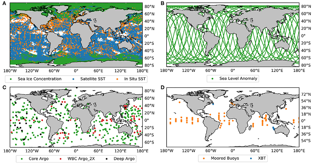
Figure 1. Examples of synthetic observations coverage on 1 June 2009: (A) sea surface temperature and sea ice concentration, (B) sea level anomaly tracks, (C) profiles from Argo floats, and (D) profiles from moored buoys and XBTs.

2.2. Observing System Simulation Experiments

The Met Office performed five OSSEs using the GO6 configuration (Storkey et al., 2018) of the operational FOAM system. The model is based on the Nucleus for European Modeling of the Ocean (NEMO) code v3.6 (Madec, 2012) and the results are on an extended ORCA grid at 1/4° resolution with 75 vertical levels. As mentioned earlier, the Nature Run was produced by Mercator Ocean using the 1/12° PSY4V3R1 system (Lellouche et al., 2018) which uses version 3.1 of NEMO. Although both systems use the same underlying ocean model, there are differences in the details of various parameterizations, the bathymetry, horizontal and vertical resolution, and atmospheric forcing. For instance, the FOAM system uses a lateral eddy diffusivity of 150 m²s⁻¹, and a horizontal bilaplacian eddy viscosity of −1.5e¹¹m⁴s⁻¹, while the Mercator PSY4 systems uses 100 m²s⁻¹ and −2e¹⁰m⁴s⁻¹, respectively. All of these differences ensure a sufficient error growth between the OSSEs and the NR and avoid unrealistic or biased impact assessments using the OSSEs.

Importantly, the OSSEs were forced by daily fluxes from the Japanese 55-year Reanalysis (JRA55), produced by the Japan Meteorological Agency (JMA) (Ebita et al., 2011; Kobayashi et al., 2015), while the NR was forced by fields from the ERA-Interim reanalysis from ECMWF. This introduces an important source of error growth between the NR and the OSSEs which reflects the operational situation where the true state of the atmosphere is unknown. The OSSEs also used a lower resolution model than the NR to introduce additional truncation errors, which is ideal for an effective OSSE set up (Halliwell et al., 2014).

The outputs from the last year (which was 2006) of a long-running free run were used to initialize the experiments. OSSEs were run for 2 years from January 2008, with the first 6 months (January–June 2008) as the spin-up period. Unless specified, results shown here are from the second year of the model run.

The data assimilation scheme used in FOAM is called NEMOVAR and is developed collaboratively by Centre Européen de Recherche et de Formation Avancée en Calcul Scientifique (CERFACS), European Centre for Medium-range Weather Forecasts (ECMWF), Institut National de Recherche en Informatique et en Automatique (INRIA), and the Met Office. NEMOVAR is implemented as a multivariate, multi-length-scale incremental 3D-Var FGAT (first-guess-at-appropriate-time) scheme (Waters et al., 2015; Mirouze et al., 2016) and is used to assimilate a range of observation types including satellite and in situ SST observations, in situ temperature and salinity profiles, satellite altimeter observations, and satellite measurements of sea-ice concentration.

Table 1 lists the observation types assimilated in each of the four OSSEs with data assimilation. A Free Run (hereafter FR) was carried out without assimilating any observations and was used to examine the systematic differences between the NEMO model run in the OSSEs and the one used to generate the NR. Backbone (hereafter BB) run assimilates observations representing the current observing network, which is used as the baseline for assessing the impact of assimilating additional in situ observations in other OSSEs. Both OSSEs and NR were interpolated to a common 1/4° grid with 50 vertical levels before statistical comparisons. The performance of each model run was assessed by calculating the mean differences (also referred to as bias, as the NR represents the true ocean state) and root mean square error (RMSE) against the NR.

TABLE 1

Table 1. OSSEs with data assimilation at the Met Office.

The synthetic observations were first tested in the Free Run, in which no observations were assimilated but instead verified by producing observation-minus-model (O-M) statistics for temperature and salinity fields. The mean differences and root mean square (RMS) of the O-M matchups were calculated and compared against those calculated from a Free Run using real observations during January–March 2008. For temperature fields (Figures 2A,B), the O-M fields verifying the synthetic observations have slightly smaller mean differences and RMS than using real observations. However, the salinity mean difference and RMS for the run using synthetic observations (bottom panel of Figure 2D) are slightly larger and more static above 300 m than using real observations (bottom panel of Figure 2C). It is worth noting that there were more synthetic observations in this test because the observations were generated using the data coverage in 2016. The difference in the number of observations should be taken into account in interpreting the results. Overall, the results from the two runs are comparable and it is safe to conclude that the synthetic observations can be used for the OSSEs.

FIGURE 2

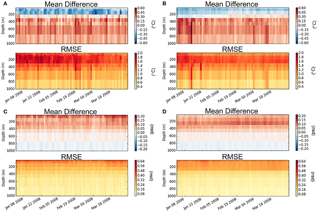
Figure 2. Hovmöller plots of observation-minus-model (O-M) statistics for temperature and salinity fields averaged over the Global Ocean from the free runs verifying real and synthetic observations during January–March 2008: (A) real temperature observations, (B) synthetic temperature observations, (C) real salinity observations, and (D) synthetic salinity observations. Each subplot includes two panels showing the mean differences in the top panel and root mean square (RMS) in the bottom panel.

3. Results

3.1. Impact of Data Assimilation

First, the impact of assimilating observations from the full current observing network was assessed by evaluating the Backbone (BB) results against the Nature Run (NR). Note, all the statistical results (referred to as OSSE statistics, e.g., BB statistics) shown in this section are calculated for OSSE-minus-NR fields, unless stated otherwise. The improvements or degradation observed in the statistics between two OSSEs are also in reference to the Nature Run. The Backbone statistics were compared to those calculated using the Free Run (FR), where the differences indicate the influence from assimilating the synthetic observations. Results shown here are averaged over the Atlantic Ocean over January–December 2009.

Figure 3 shows the mean difference and RMSE for the Free Run and the Backbone temperature fields, both in reference to the Nature Run. The Free Run is warmer than the NR at the surface but colder between the surface and 1,000 m. These biases are largely reduced in the BB statistics (Figure 3B), although the Backbone still remains warmer than the Nature Run in the top 200 m. At around 1,000 m, the Backbone run shows intensified warm biases compared to the Free Run. This requires further investigation, but overall the mean differences for temperature are reduced significantly by assimilating observations. Noticeable RMSE reduction is seen in the top 500 m for the Backbone field compared to the Free Run (Figures 3C,D), although the RMSE is still larger than the layers below.

FIGURE 3

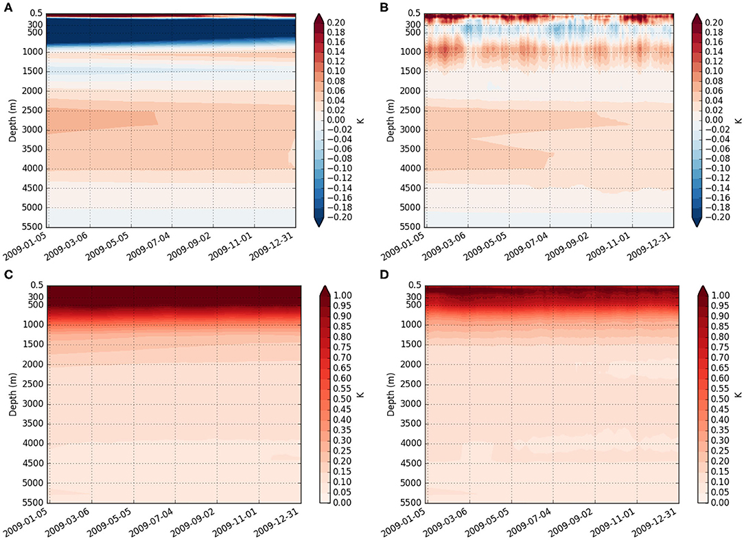
Figure 3. Hovmöller plots of OSSEs-NR statistics for temperature field in the Atlantic over January–December 2009: (A) Free Run bias, (B) Backbone bias, (C) Free Run RMSE, and (D) Backbone RMSE.

Figure 4 shows the same comparison but for salinity. The Free Run is much fresher than the Nature Run in the top 500 m but saltier between 500–2,000 m (Figure 4A). These biases are largely reduced in the Backbone run, although it remains fresher than the Nature Run in the top-most layer (Figure 4B). This fresh bias in the top layer is possibly related to the different surface forcing used in the OSSEs and the Nature Run: the OSSEs used JRA55 fluxes while the Nature Run was forced by the ERA-interim products. Previous studies have found that JRA55 fluxes are noticeably different to the ERA-Interim fluxes (Kubota and Tomita, 2015; Wang et al., 2016). This was a deliberate choice so the surface forcing used in the OSSEs are not too close to truth, which would be unrealistic. This choice also makes sure the OSSE results are not biased due to insufficient error growth rate between the OSSEs and the Nature Run by using the same surface forcing (Halliwell et al., 2014). It is also worth mentioning that the results suggest assimilating Argo observations is not sufficient to correct the errors in the surface forcing. Satellite observations of surface salinity could be useful for constraining sea surface salinity in ocean forecasting systems (Martin et al., 2019). Assimilating salinity observations also reduces the Backbone RMSE, especially for the depths between 500 and 1,000 m, where the large RMSE in the Free Run has been reduced. Above 500 m, the RMSE is still around 0.1 in Backbone run and is much larger than the depths below.

FIGURE 4

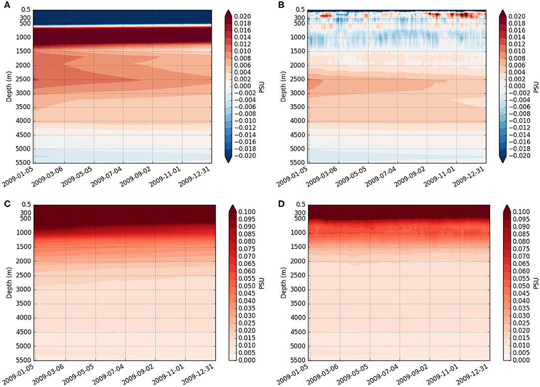
Figure 4. Hovmöller plots of OSSEs-NR statistics for salinity field in the Atlantic over January–December 2009: (A) Free Run bias, (B) Backbone bias, (C) Free Run RMSE, and (D) Backbone RMSE.

It is clear that by assimilating observations, the bias and RMSE seen in the Free Run fields are largely reduced in the Backbone run. The overall BB temperature bias is <0.3 °C and salinity bias is <0.2 psu in the Atlantic. Figure 5 shows the annually averaged Backbone RMSE for temperature and salinity fields at 100 m. Larger temperature RMSE are mainly observed in regions with active circulation or turbulence, e.g., the Western Boundary Current (WBC) and prevailing westerly regions. The salinity RMSE also shows higher values around the WBC regions, although the largest RMSEs are observed in the polar region in the Northern Hemisphere, where the freezing and melting of sea ice introduces more uncertainties. The results show that the distribution and range of the RMSE for Backbone temperature and salinity fields are reasonable, and large RMSEs can be traced back to system differences.

FIGURE 5

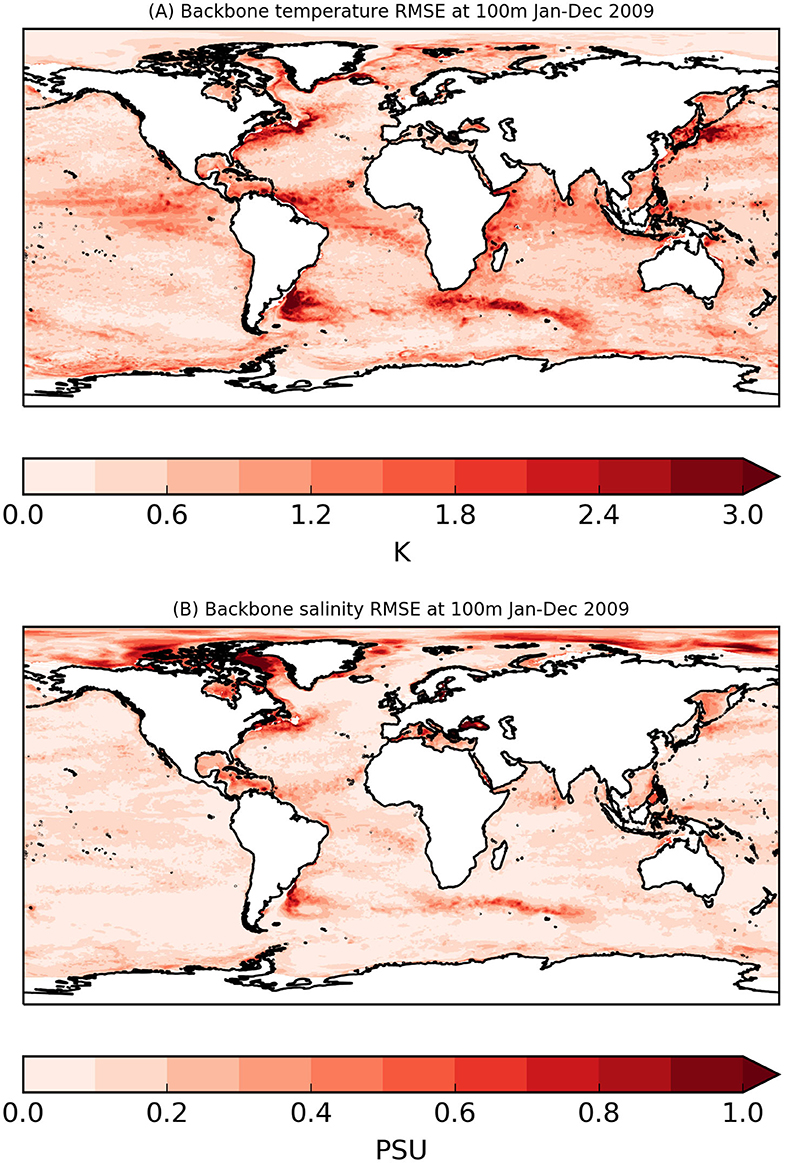
Figure 5. The spatial map of annually averaged Backbone RMSE (relative to the Nature Run) for (A) temperature and (B) salinity fields at 100 m depth.

3.2. Impact of Adding Extra Observations

In this section, the impacts of assimilating extended Argo profiles and removing mooring profiles are examined in three OSSEs. Similar to the previous section, the impacts are assessed by validating the model outputs against the Nature Run. OSSE results are then compared to Backbone run statistics, which are used as the baseline for the additional OSSEs. All statistical results are calculated in reference to the NR. As some of the additional observations are distributed in certain regions of the globe, results in this section are regional averages. The AtlantOS project defined basin scale and WBC regions to be used for regional analysis, but Figure 6 only shows the regions used in this study.

FIGURE 6

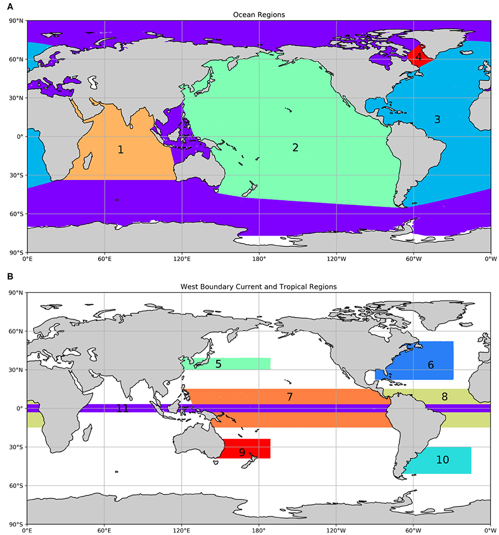
Figure 6. The regions used to assess the impacts of additional or removal of observations: (A) ocean basin wide regions and (B) western boundary current regions included in the paper: 1. Indian Ocean, 2. Pacific Ocean, 3. Atlantic Ocean, 4. Labrador Sea, 5. Kuroshio Current, 6. Gulf Stream and extension, 7. Tropical Pacific, 8. Tropical Atlantic, 9. East Australian Current, 10. Brazil Current, and 11. Equator.

3.2.1. Impact of Adding ARGO_2X Floats

The WBC_ARGO2X run assimilated the same observations as the Backbone run, but with additional Argo profiles added in WBC regions as well as along the equator (between 3°N and 3°S), to achieve two profiles per 3° × 3° box per 10 days in these regions. The distribution and procedure for creating the ARGO_2X profiles are detailed in Gasparin et al. (2019). An example of the distribution of the ARGO_2X profiles is shown in Figure 1C for 1 June 2009. In this section, we present results of WBC_ARGO2X against the Backbone results, both in reference to the NR, in the Gulf Stream and a few other WBC regions.

One way to assess the impact of including ARGO_2X floats is to compare the RMSE of the OSSEs with and without these floats. This is achieved by calculating the RMSE reduction of WBC_ARGO2X compared to the Backbone run following Equation (3) below:

• Calculate temporally averaged mean square at each grid point

$\begin{array}{ll}M{S}_{i,j,z}=\frac{\sum \left({\displaystyle x_{i,j,z,t}^2}\right)}{N}& (1)\end{array}$

where x_{i, j, z, t} is the daily OSSE-NR value at grid point (i, j), depth z and day t. N is the number of days.

• Calculate weighted geographical averaged RMSE

$\begin{array}{ll}RMS{E}_z=\frac{\sum \left(\sqrt{M{S}_{i,j,z}}\right)}{Are{a}_{weighted}}& (2)\end{array}$

• Calculate RMSE reduction using the following equation:

$\begin{array}{ll}100\times ({\text{BB-NR}}_{\text{RMSE}}-{\text{OSSE-NR}}_{\text{RMSE}})/{\text{BB-NR}}_{\text{RMSE}}& (3)\end{array}$

The RMSE reduction ratio is calculated for each depth. A positive ratio indicates that the OSSE being tested performs better than the Backbone run (BB) in reference to the Nature Run (NR), whilst a negative ratio suggests degradation in the OSSE.

From Figure 7, it is clear that by adding the ARGO_2X profiles, the RMSE is reduced in WBC_ARGO2X compared to the BB run, with a positive ratio across the whole depth for temperature and salinity fields. In most regions, the RMSE reduction ratio is around ~10%, with the maximum ratio close to 15% in the Kuroshio Current area at 900–1,100 m depths. It is worth noting that although the RMSE reduction ratio is larger below 1,000 m, the actual RMSE values are much smaller (e.g., Figure 7B). Over time, there are also variations of improvements and degradation in the temperature and salinity fields (not shown). Both the Backbone and WBC_ARGO2X runs are colder and fresher than the Nature Run at the very top layer of the water column. The cold and fresh bias is reduced in WBC_ARGO2X but not consistently through the whole of 2009, for example, an intensified cold bias is seen from September 2009 onward. Below the surface, both the Backbone and WBC_ARGO2X are warmer than the Nature Run and WBC_ARGO2X shows reduced warm bias from May 2009 onward. Mixed improvements and degradation are seem for the temperature fields between 100 and 800 m in WBC_ARGO2X compared to the Backbone. For salinity, improvements in WBC_ARGO2X are mainly seen at depths with fresh bias against the Nature Run, but similar to the temperature, mixed improvements and degradation are seen in the salinity field.

FIGURE 7

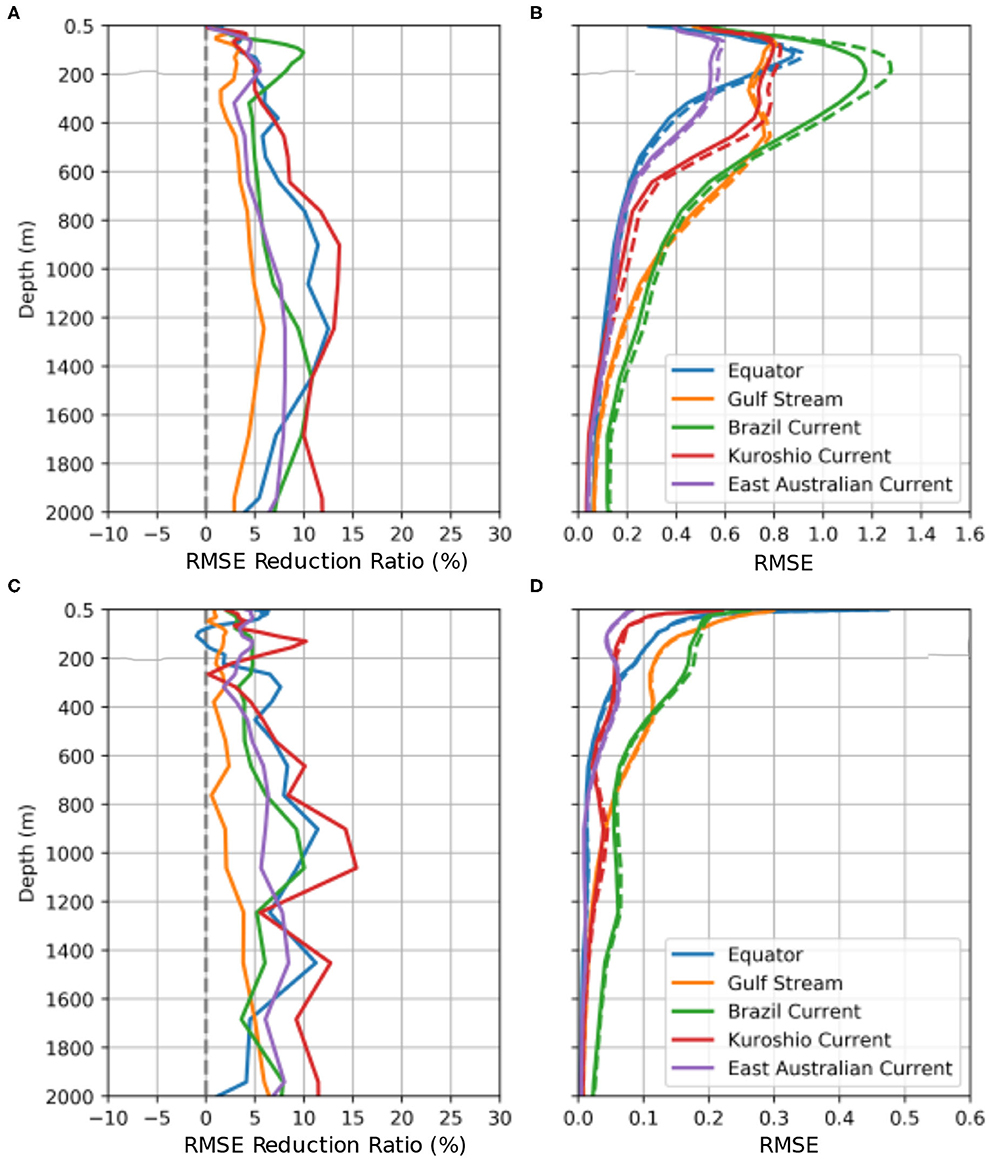
Figure 7. RMSE reduction (as defined by Equation 3) and RMSE of WBC_ARGO2X-NR compared to Backbone-NR in five geographical regions: (A) temperature RMSE reduction ratio, (B) temperature RMSEs of WBC_ARGO2X (solid lines) and Backbone (dashed lines), (C) salinity RMSE reduction ratio, and (D) salinity RMSE of WBC_ARGO2X (solid lines) and Backbone (dashed lines). Blue: Equator, orange: Gulf Stream, green: Brazil Current, red: Kuroshio Current and purple: East Australian Current.

Additional ARGO_2X floats may also alter the representation of the Gulf Stream with additional constraints to the surface and subsurface velocities. Figure 8 shows the annual mean Gulf Stream current speeds from the Backbone and WBC_ARGO2X runs (and their differences), together with the observation-derived GlobCurrent v3.0 product (Rio et al., 2014) over 2009. The average currents from the Free Run and the Nature Run are also presented in Figure 8 as reference. Note, the currents for the NR were calculated using regridded data on ORCA 1/4° resolution, the velocity data on ORCA 1/12° resolution were not provided for the project. Both the Backbone and WBC_ARGO2X capture the main Gulf Stream pathway relatively well, although neither captures it perfectly. WBC_ARGO2X shows slightly strengthened currents along the Gulf Stream Extension area southeast of Newfoundland and agrees better with the observation-derived product which shows much stronger currents in this area. The meandering of the Gulf Stream in the WBC_ARGO2X also matches better to the NR than the Backbone run, with more established structure of the eddies although both runs show weaker currents in the Gulf Stream Extension area than in the NR. The Nature Run shows stronger currents in the northeast stretch of the Gulf Stream Extension area than in the observation-derived product, but still show weaker currents in the area southeast to Newfoundland. Compared to the observation-derived product and other runs, the main pathway of the Gulf Stream in the Free Run is much closer to the continent, which is corrected in the Backbone and WBC_ARGO2X runs. This gives confidence that the operational system can correct the position of the Gulf Stream and that additional observations will lead to further improvements.

FIGURE 8

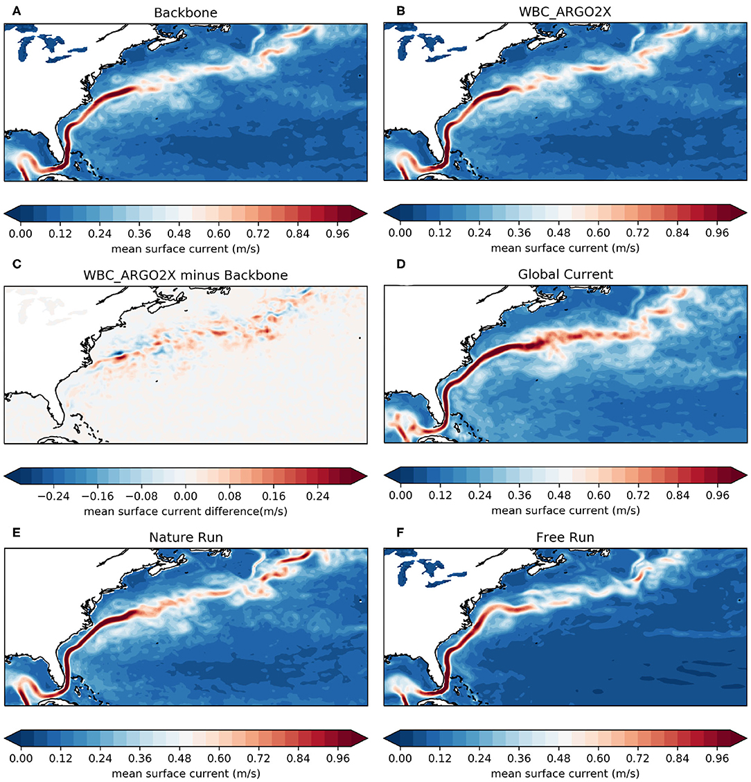
Figure 8. Annual mean surface current speed over 2009 for: (A) the Backbone, (B) the WBC_ARGO2X, (C) the WBC_ARGO2X minus the Backbone differences, (D) the observation-derived GlobCurrent v3.0 surface currents product (Rio et al., 2014) (E) the Nature Run, and (F) the Free Run.

3.2.2. Impact of Adding Deep Argo

The DEEP run assimilated profiles from simulated deep Argo profiles in addition to the same observations in the Backbone run. The deep Argo profiles were constructed by extending ~1/3 of the ARGO_1X profiles to around 5,500 m. The resulting deep Argo array reports monthly and has one profile per 5° × 5° box (Gasparin et al., 2019). Similar to the analysis of the WBC_ARGO2X run, this section presents DEEP statistics against those calculated using the Backbone run. All results are produced in reference to the Nature Run. The synthetic deep Argo floats are distributed evenly across the globe. Therefore, the impacts of these profiles are examined in basin scale regions, as well as in regions where deep convection occurs. Figure 9 shows the RMSE reduction ratio calculated following Equation (3).

FIGURE 9

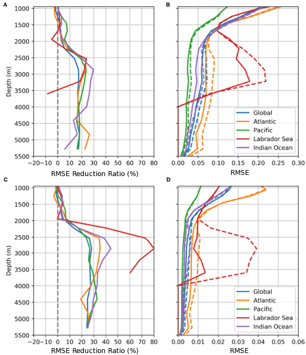
Figure 9. RMSE reduction (as defined by equation 3) and RMSE of DEEP-NR compared to Backbone-NR in five geographical regions: (A) temperature RMSE reduction, (B) temperature RMSE of DEEP (solid lines) and Backbone (dashed lines), (C) salinity RMSE reduction, and (D) salinity RMSE of DEEP (solid lines) and Backbone (dashed lines). Blue: Global, orange: Atlantic, green: Pacific, red: Labrador Sea and purple: Indian Ocean.

For temperature, the improvements in DEEP RMSE against the Backbone run are most noticeable below 2,500 m, for all regions the reduction rate is around 20% at that depth. Note the Labrador Sea is ~3,400 m deep so the Deep Argo measurements only go down to the model level closest to 3,400 m and the RMSE for these profiles are much larger than the other regions, see Figure 9B. For salinity, RMSE reduction is neutral above 2,000 m in all regions. Below 2,000 m, all regions except for the Labrador Sea have a positive reduction ratio of around 30%. In the Labrador Sea, the ratio reaches 80% at ~3,000 m. The Backbone RMSE value in the Labrador Sea is about four times the size of the RMSEs in the other regions below 2,000 m, whilst the DEEP RMSE value is about the same size as in the other regions, confirming the positive impact from assimilating deep Argo.

However, some degradation around 1,000 m is seen in the DEEP statistics, for both temperature and salinity fields. The exact reasons for the degradation of the DEEP statistics around 1,000 m require further investigation, but one potential explanation is that the model also assimilated sea level anomaly (SLA) observations from the altimeters, which modified the properties of the water column. When assimilating additional deep Argo observations, the interaction between SLA and deep Argo profiles could cause the undesirable effects seen at depths shallower than 2,000 m. This highlights a potential direction for future development of the assimilation scheme for better use of deep Argo profiles. The overall results of assimilating deep Argo profiles are very promising, especially below 2,500 m, suggesting the deployment of deep Argo floats would provide valuable information about the deep ocean and hence should be considered in the future observing network design.

3.2.3. Impact of Removing Moorings

The impact of the mooring arrays in FOAM was tested in a withdrawal experiment, in which the profiles from moorings were removed from the synthetic observations used in the Backbone run. This withdrawal experiment aims to examine the importance of the moored arrays in ocean analysis, especially in the tropical regions where long-term moored buoys are deployed. Compared to an Observing System Experiment (OSE), in which withdrawal experiments are often conducted, an OSSE allows the experiments with or without moorings to be compared in reference to the “true” ocean state provided by the Nature Run. These moorings are mainly distributed in the tropics, north-western Atlantic, western Pacific, and the Indian Ocean. The real mooring locations in 2015 were used to represent the mooring sampling during the OSSE period, as 2015 is considered one of the most representative periods in the Global Tropical Moored Buoy Array (Gasparin et al., 2019).

The Tropical Atmosphere Ocean (TAO) Arrays in the tropical Pacific and the Prediction and Research Moored Array in the Tropical Atlantic (PIRATA) in the tropical Atlantic are two of the most successful mooring projects for monitoring the ocean and atmosphere for climate studies. Oke et al. (2015) reported that the TAO/PIRATA data have equivalent impacts to Argo floats on ocean forecasting system within 10 degrees of the equator. More recently, the Research Moored Array for African-Asian-Australian Monsoon Analysis and Prediction (RAMA) array was deployed in the tropical Indian Ocean under the Climate Variability and Predictability (CLIVAR) Project (Ballabrera-Poy et al., 2007). To best demonstrate the impact of removing mooring profiles, this section focuses on the Equatorial areas, covering the tropical regions within 3°N and 3°S across all ocean basins, tropical Atlantic, tropical Pacific, and the Indian Ocean. Similar to previous sections, the NoMoor RMSE is compared to the Backbone run and all statistics are in reference to the Nature Run.

The RMSE reduction ratio was calculated in the same manner as for previous experiments and is show in Figure 10. For the temperature fields, most of the degradation in the NoMoor run is seen in the top 400 m for all selected regions. In the Equatorial region and tropical Pacific, the degradation penetrates deeper to about 600 m. Below 600 m, however, most regions show improvements in RMSE in the NoMoor run compared to the Backbone run, except for the tropical Atlantic between 1,000 and 1,600 m. For salinity fields, a small degradation is seen in the top 100 m in the Equatorial region and the tropical Pacific, before the ratio turns positive between 100 and 200 m, indicating improvements in RMSE in the NoMoor run. Below 400 m, not much changes in the RMSE with or without mooring profiles in the Indian Ocean; mixed degradation and improvements are seen in the tropical Atlantic and Equatorial region. The tropical Pacific shows consistent improvements below 600 m, which is surprising and requires further investigation to fully understand the reasons. It is worth noting that the magnitudes of improvements or degradation are smaller in the NoMoor run compared to the DEEP or WBC_ARGO2X runs. The degradation seen near the surface is around 2.5% and the maximum RMSE change ratio is about 5%.

FIGURE 10

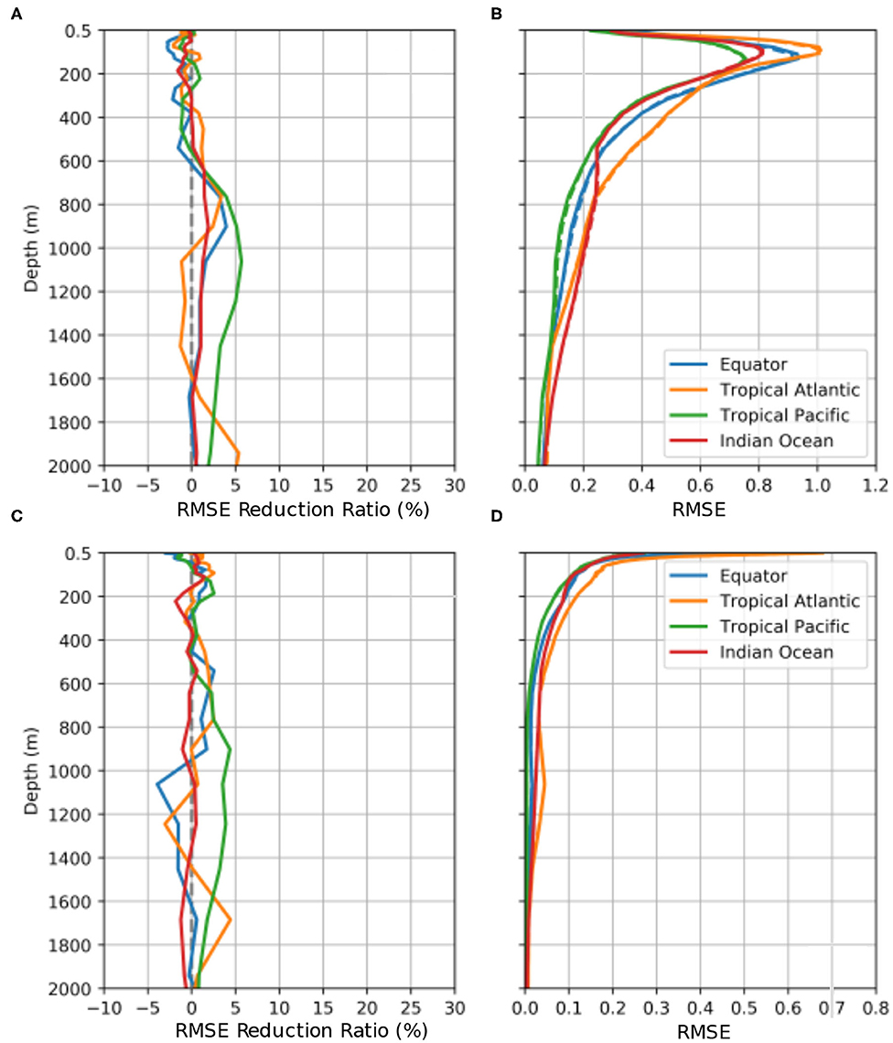
Figure 10. RMSE reduction (as defined by Equation 3) and RMSE of NoMoor-NR compared to Backbone-NR in four geographical regions: (A) temperature RMSE reduction, (B) temperature RMSE of NoMoor (solid lines) and BB (dashed lines), (C) salinity RMSE reduction, and (D) salinity RMSE of NoMoor (solid lines) and BB (dashed lines). Blue: Equator, orange: Tropical Atlantic, green: Tropical Pacific, red: Indian Ocean.

3.3. Impact of Additional Observations on SSH Variability, OHC, and AMOC

In addition to directly influencing the temperature and salinity fields by adding or removing an observation type, the impacts are expected to extend to derived variables that are closely linked to temperature and salinity fields. This section explores the potential impacts of the observations on the Ocean Heat Content (OHC) and the Atlantic Meridional Overturning Circulation (AMOC). As discussed in previous sections, the influence from the moorings is very localized with limited impact in regional statistics. Therefore, this section focuses on the two experiments where 10–20% RMSE improvements are observed in temperature and salinity fields: DEEP and WBC_ARGO2X runs.

We also investigated the impact of the observing network changes on the sea-surface height (SSH) variability, but found that while the SSH variability is well-represented in the Backbone experiment compared to the Nature Run, there is little benefit from the additional observations. This is not unexpected given that the horizontal spacing of Argo floats is much greater than the length-scale of mesoscale eddies. However, proposed changes to the global observing system, such as the use of wide-swath altimeter observations (Morrow et al., 2019), would be expected to improve this as they will in future provide two-dimensionally resolved observations of the sea surface height.

3.3.1. Impact on Ocean Heat Content

The OHC variation during the spin-up period indicates how the assimilation of observations constrain the model, therefore the timeseries for the entire 2-year period are shown here, however results from the first 8 days are excluded due to a problem in the Nature Run.

Figure 11 shows the OHC between 300 and 700 m for the Nature Run, Free Run, Backbone, and WBC_ARGO2X experiments in four Western Boundary Current regions. The depth ranges were agreed between participating institutes in the AtlantOS project to allow inter-comparison of results, the other depth ranges are 0–300, 700–2,000, 2,000–4,000, 0–2,000, and 4,000 m–bottom. These depth ranges are commonly used for studying OHC, as 0–300 m corresponds to the depths covered by older types of profile instruments, 700 m is the depth limit for the XBTs commonly used since the 1990s and 2,000 m corresponds to the depth limit of the core Argo floats. For the impact of the ARGO_2X profiles, the 300–700 m range is selected as it avoids the surface where the OHC is dominated by the different fluxes used to force the Nature Run and the OSSEs. The depth range also demonstrates the OHC variability in the NR best as the variability is much smaller in the Nature Run for depth ranges below 700 m in the regions of interest. In the Gulf Stream and Brazil Current regions (Figures 11A,C), there is a clear model drift over the 2-year period without data assimilation (Free Run shown in yellow). With assimilation, this drift is corrected in both the Backbone and WBC_ARGO2X runs (green and red lines, respectively). In the Kuroshio Current and East Australian Current regions (Figures 11B,D), the model drift is less pronounced and all four experiments show similar long-term variability in OHC. Overall, it appears that assimilation corrects the magnitude of the OHC toward the Nature Run, but introduces spurious variability. The impact of the additional Argo observations in the WBC_ARGO2X run does not appear to be large, but in the East Australian Current region at least, WBC_ARGO2X is in better agreement than the Backbone run with the Nature Run OHC.

FIGURE 11

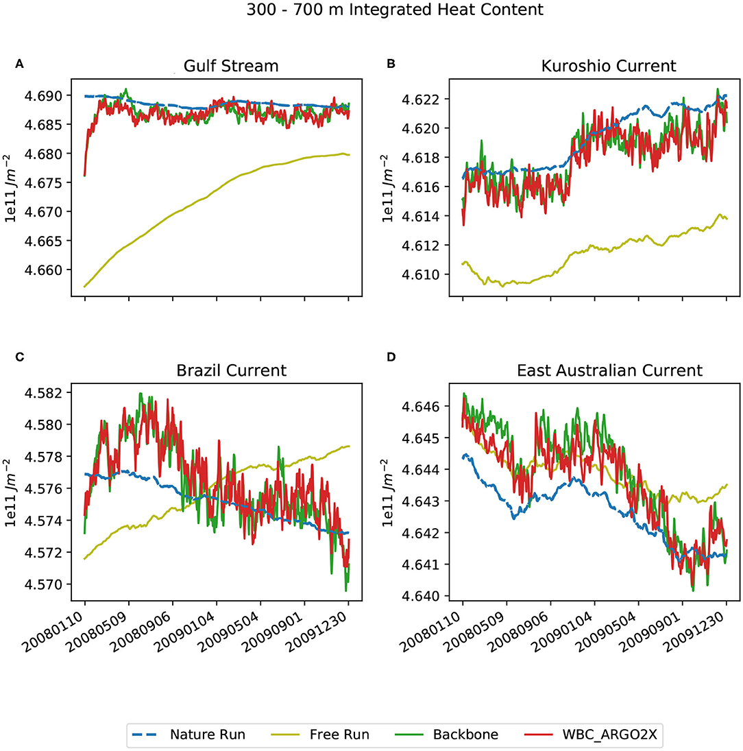
Figure 11. The Ocean Heat Content between 300 and 700 m for the Nature Run (dashed blue lines), Free Run (yellow), Backbone (green), and WBC_ARGO2X (red). The results were averaged over the Gulf Stream (A), Kuroshio Current (B), Brazil Current (C), and East Australian Current regions (D).

The OHC between 2,000 and 4,000 m for the Nature Run, Free, Backbone, and DEEP runs are shown in Figure 12. In most regions, the OHC does not vary much in the Nature Run over the 2-year period at these depths, except at the Equator where an annual signal is observed (dashed blue lines in Figure 12E). A model drift is seen in the Free Run OHC in most regions. In the Equatorial region, although the Backbone experiment appears to be closer to the Nature Run around late-2008, neither experiment is consistently closest to the Nature Run in this region. However, the long-term OHC trend in the Free Run (relative to the Nature Run) is removed by assimilation in the Backbone and DEEP runs. By the start of the second year (January 2009) the additional deep Argo observations in the DEEP run appear sufficient to correct the average magnitude of the OHC in the Indian and Pacific Ocean basins. This demonstrates the potential for future deployment of deep-Argo to constrain the heat content of the deep ocean with one-third of the Argo network profiling the deep ocean every month.

FIGURE 12

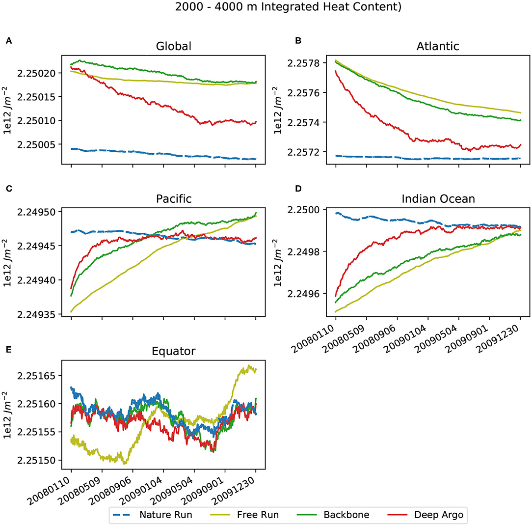
Figure 12. The Heat Content between 2,000 and 4,000 m for the Nature Run (dashed blue lines), Free Run (yellow), Backbone (green), and Deep Argo (red). The results were averaged over Global Ocean (A), Atlantic (B), Pacific (C), Indian Ocean (D), and Equator (E).

3.3.2. Impact on Meridional Overturning Circulation

Average Atlantic Meridional Overturning Circulation (AMOC) was calculated for the FOAM OSSEs over the 2-year model run. The transport is calculated from the meridional residual mean velocity and is presented as a function of latitude. The calculation was adapted from the CMIP6 settings and Equation (I6) in (Griffies et al., 2016):

$\begin{array}{ll}\text{Ψ}(y,t)=-{\displaystyle {\int }_{x_a}^{x_b}}dx{\displaystyle {\int }_{-H}^Z}{\rho }_{0}vdz,& (4)\end{array}$

where x and y are the directions defined according to the model native grid, H and Z are the depths over which the streamfunction is calculated, ρ₀ is the water mass density, v is the meridional residual mean velocity and Ψ is the transport stream function for the steady-state rigid-lid Boussinesq case.

Key information required to calculate the AMOC was not produced in the Nature Run so it was not possible to compare the AMOC signal of the OSSEs against the NR. Figure 13A hence only shows the average AMOC in the Atlantic ocean in FOAM OSSEs (Free Run, Backbone, DEEP, and WBC_ARGO2X runs). The AMOC features agree well with the AMOC depicted by reanalyses (Jackson et al., 2019). In the Free Run (Figure 13A), the northward volume transport is observed between 30 °S and 60 °N and a much weaker southward return flow is seen below 3,000 m. The maximum northward transport, close to 30 Sv, is located around the Equator at ~1,000 m. With data assimilation, the maximum transport center in the Backbone run (Figure 13B) shifts to just north of the Equator and the stream function shows discontinuities near the Equator. This is a known issue in some ocean models due to the assimilation scheme, e.g., Jackson et al. (2019) suggested the issue seen in GloSea5 is due to the assimilation of sea surface height. GloSea 5 also uses the 3D-Var NEMOVAR assimilation for ocean and sea ice components (Maclachlan et al., 2015). It is also very difficult to perform satisfactory data assimilation at the Equator without generating vertical flows due to the difficulties to maintain the balance between the ocean pressure gradients and the applied wind stress near the ocean surface in this region when increments are applied to an ocean model (Waters et al., 2017). With additional Deep Argo observations (Figure 13C), the southward return flow below 3,000 m is strengthened, although the discontinuities in the stream function at the Equator intensify in the upper 2,000 m. This indicates that assimilating Deep Argo profiles leads to noticeable changes in the average AMOC at the expected depths, although further assimilation development is required to resolve the discontinuities of the stream function at the Equator. The added WBC Argo floats (Figure 13D) have little impact on the AMOC compared to the Backbone, possibly because these floats are located only in the WBC regions and are mostly distributed in the upper 2,000 m. The only noticeable impacts include slightly reduced northward volume transport in the upper ocean and a smaller maximum transport center for the upper cell.

FIGURE 13

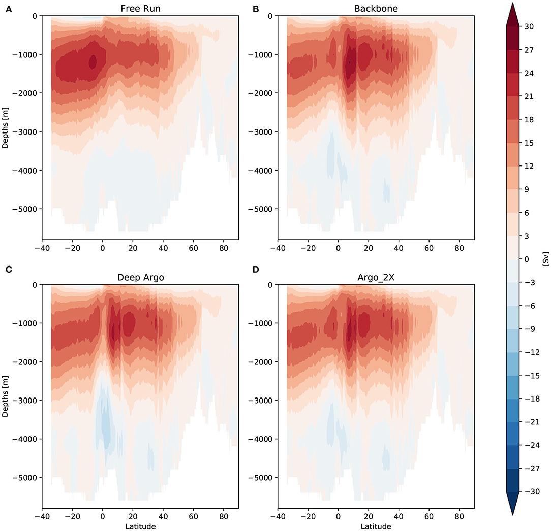
Figure 13. The average Atlantic Meridional Overturning Circulation (AMOC) during 9 January 2008–31 December 2009: (A) AMOC in the Free Run, (B) AMOC in the Backbone run, (C) AMOC in the Deep Argo run, and (D) AMOC in the WBC_ARGO2X run.

The timeseries of the vertical maximum volume transport at 26.5°N over the 2-year model run are shown in Figure 14. The timeseries are comparable between the four runs, with the Free Run showing slightly weaker volume transport at the beginning of the timeseries. The transports in all runs are steady over most of the period and toward the end of 2009, the northward transports are noticeably reduced. This period falls in the declining phase of the AMOC, previously observed and reported from the RAPID array (McCarthy et al., 2012; Smeed et al., 2014). The timeseries confirm the feature seen in Figure 13, that the northward flow remains similar between the two OSSEs with the additional Argo profiles assimilated.

FIGURE 14

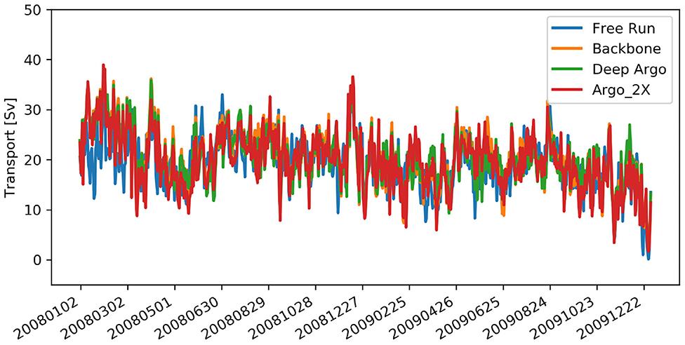
Figure 14. Daily vertical maximum AMOC transport at 26.5 °N during 9 January 2008–31 December 2009 in Free Run, Backbone, Deep Argo, and WBC_ARGO2X run.

4. Discussion and Conclusions

This paper assessed the impact of assimilating observations in the FOAM ocean forecasting system from an OSSE perspective. More specifically, the benefits from assimilating additional in-situ observations and the importance of a well-designed observing network. A set of synthetic observations were produced from the Nature Run, produced by Mercator Ocean as part of the Horizon 2020 AtlantOS project. As part of this project, OSSEs were carried out at the Met Office using the FOAM system and the synthetic observations for the period of 2008–2009.

Statistical comparisons between the Free Run and the Nature Run indicated that the differences between the two versions of the model (including resolution and surface forcing differences) are mainly seen in the top 1,000 m. Generally the Free Run is warmer and fresher near the surface than the Nature Run. The fresh biases at the very top layer of the water column are related to the different surface flux products used to force the two models. By assimilating observations from the full observing network, the biases and RMSEs of temperature and salinity fields are significantly reduced in the Backbone compared to the Free Run. This indicates that the NEMOVAR data assimilation scheme is effective in utilizing observations to reduce model errors and FOAM can better represent the true ocean state by assimilating existing observations.

Three more OSSEs were completed to test the impacts of adding or removing observations with the aim of improving the design of the future in-situ observing networks for reanalysis, analysis and forecasting of the ocean. The WBC_ARGO2X run assessed the benefit of doubling the sampling frequency of Argo floats in the Western Boundary Currents and equatorial regions. With the additional Argo profiles, the RMSE of the WBC_ARGO2X run is reduced by ~10% compared to the Backbone RMSE in WBC regions and the Equator. The improvement is more uniform across the regions for temperature than for salinity. It is clear that assimilating observations is vital in constraining the models and correcting the model drift seen in the Free Run. However, the impact on the Ocean Heat Content estimation of the extra Argo observations in the WBCs is less clear, but there is some improvement in the East Australian Current region.

The core Argo floats normally measure the water column down to 2,000 m. The DEEP run provided an opportunity to assess the potential benefits from assimilating Deep Argo profiles with measurements below 2,000 m. The improvements in the biases and RMSE in the DEEP experiment (relative to the Nature Run) are clear for temperature and salinity fields in the Atlantic, especially between 2,000 and 4,000 m. The DEEP RMSE is reduced by around 20–25% compared to the Backbone RMSE in most regions. In the Indian Ocean, the salinity RMSE reduction reaches 40% around 3,000 m and in the Labrador Sea, the salinity RMSE reduction can reach 80%. Assimilating deep Argo profiles also leads to further modification of the MOC below 2,000 m, although the discontinuities of the stream function near the Equator appears to have intensified in the DEEP run. The magnitude of the OHC in the deep ocean (below 2,000 m) is significantly improved in all ocean basins when assimilating deep Argo observations. However, assimilating deep Argo observations degraded the temperature and salinity RMSEs against the Nature Run above 1,500 m. This could be due to the interactions between SLA and deep Argo not being resolved properly by the current data assimilation scheme. Future development would be beneficial to make better use of the deep Argo observations.

The long-term mooring projects in the tropical oceans have provided valuable information for understanding the ocean and atmosphere conditions. The observations have proved to be crucial in constraining ocean models for operational ocean forecasting, seasonal forecasting and climate studies in the tropics (e.g., Ballabrera-Poy et al., 2007; Fujii et al., 2015; Xue et al., 2017b), as well as being a useful tool for model and satellite data validation (e.g., Bentamy et al., 2006; Tang et al., 2014). By removing the mooring profiles from the system, an overall degradation in biases and RMSEs is seen for temperature and salinity fields at the Equator. However, some improvements are seen when with-holding the mooring observations, for example during October–December 2009 in the temperature field at the surface and during January–March 2009 in the subsurface salinity field.

Compared to the Backbone RMSE, the NoMoor RMSE changes are within ± 5% in the tropical regions. One surprising result is the improvement in RMSE of ~5% in the Tropical Pacific, especially considering the success of TAO and the later Triangle Trans-Ocean Buoy Network (TRITON) arrays in providing oceanic and atmospheric information over the past decades. It has been previously reported that within 10 degrees of the equator, mooring profiles are as important as Argo floats in reducing model errors, although the impact from moorings are more localized than the Argo floats (Oke et al., 2015; Xue et al., 2017b). One possibility is the fact that the number of mooring observations is much smaller than other types of observations such as satellites and the core Argo floats, hence the impact from the moorings could be dominated by these observations. The NoMoor results also depend on the effectiveness of the data assimilation scheme in utilizing mooring observations. It is also possible that future model development could make better use of the mooring data. The importance of the moorings should not be underestimated and the design of the mooring locations could be essential to ensure the effectiveness of the mooring observations. The Tropical Pacific Observing System (TPOS) 2020 project reached a similar conclusion that moorings are essential in constraining temperature fields in ocean analyses, as the current Argo coverage alone is not sufficient to achieve this in the tropical Pacific (Fujii et al., 2019; Kessler et al., 2019a). They also highlight that moorings provide good temporal coverage of a variety of oceanographic, atmospheric and biogeochemical variables and direct velocity measurements. Better communication with experts in ocean modeling and data assimilation during the design of mooring sites would promote better use of the mooring data in ocean analyses, as some ocean data assimilation systems tend to overfit the fixed mooring observations. This could lead to a state estimate that is too localized to the moorings and cause dynamic inconsistency and spurious variability at larger scales (Sivareddy et al., 2017; Xue et al., 2017a; Kessler et al., 2019a).

From the OSSEs performed at the Met Office using the FOAM system, we conclude that FOAM produces realistic analyses of the ocean state by assimilating observations. Additional observations provide further improvements to the analysis, especially the deep Argo floats. The impacts of these additional observations are also manifested in the OHC and AMOC, with the deep Argo observations correcting the model drift in OHC below 2,000 m.

The study also points out potential directions for future model developments. For example, the interactions between assimilating SLA and deep Argo profiles need to be addressed better to avoid degradation of the model performance for the top 1,000 m. The discontinuities in the AMOC at the Equator is intensified with the assimilation of additional Deep Argo profiles. Effective utilization of the observations, together with a well-designed ocean observing network, are key factors in monitoring the ocean variability and providing more accurate ocean analyses from daily to decadal time scales.

Data Availability Statement

The datasets presented in this article are not readily available because data volumes prevent them being made easily accessible. Requests to access the datasets should be directed to Y2hvbmd5dWFuLm1hbyYjeDAwMDQwO21ldG9mZmljZS5nb3YudWs=.

Author Contributions

MM, RK, SG, and CM: conceptualization. MM, RK, SG, CM, and RR: methodology. CM, RK, and RR: software. CM: formal analysis. CM and RR: writing—original draft preparation. CM, RK, MM, and SG: writing—review and editing. CM and RK: visualization. All authors have read and agreed to the published version of the manuscript.

Funding

This project received funding from the European Union's Horizon 2020 Research and Innovation Program under grant agreement no. 633211 (AtlantOS). This work also benefited from support from the Copernicus Marine Environment Monitoring Service (CMEMS) Global Coupled Monitoring and Prediction Service (GLOCOMAPS) project. CMEMS is implemented by Mercator Ocean in the framework of a delegation agreement with the European Union.

Conflict of Interest

The authors declare that the research was conducted in the absence of any commercial or financial relationships that could be construed as a potential conflict of interest.

Acknowledgments

The authors would like to thank colleagues at the Mercator Ocean International, especially Florent Gasparin for providing additional data from the Nature Run. The authors also would like to thank Daley Calvert from the Met Office for providing tools to calculate Ocean Heat Content and Meridional Overturning Circulation.

References

Argo (2020). Argo Float Data and Metadata From Global Data Assembly Centre (Argo GDAC).

Ballabrera-Poy, J., Hackert, E., Murtugudde, R., and Busalacchi, A. J. (2007). An Observing system simulation experiment for an optimal moored instrument array in the tropical Indian Ocean. J. Clim. 20, 3284–3299. doi: 10.1175/JCLI4149.1

CrossRef Full Text | Google Scholar

Bentamy, A., Girard-Ardhuin, F., Croizé-Fillon, D., and Queffeulou, P. (2006). Validation and Analysis of Ocean Parameters Using ASCAT Data. Technical report, IFREMER.

Google Scholar

Blockley, E. W., Martin, M. J., McLaren, A. J., Ryan, A. G., Waters, J., Lea, D. J., et al. (2014). Recent development of the Met Office operational ocean forecasting system: an overview and assessment of the new Global FOAM forecasts. Geosci. Model Dev. 7, 2613–2638. doi: 10.5194/gmd-7-2613-2014

CrossRef Full Text | Google Scholar

Bryden, H. L., King, B. A., McCarthy, G. D., and McDonagh, E. L. (2014). Impact of a 30% reduction in Atlantic meridional overturning during 2009–2010. Ocean Sci. 10, 683–691. doi: 10.5194/os-10-683-2014

CrossRef Full Text | Google Scholar

Cao, C., De Luccia, F. J., Xiong, X., Wolfe, R., and Weng, F. (2014). Early on-orbit performance of the visible infrared imaging radiometer suite onboard the suomi national polar-orbiting partnership (S-NPP) satellite. IEEE Trans. Geosci. Remote Sens. 52, 1142–1156. doi: 10.1109/TGRS.2013.2247768

CrossRef Full Text | Google Scholar

Cummings, J. A. (2006). Operational multivariate ocean data assimilation. Q. J. R. Meteorol. Soc. 131, 3583–3604. doi: 10.1256/qj.05.105

CrossRef Full Text | Google Scholar

Delworth, T. L., and Zeng, F. (2016). The impact of the North Atlantic Oscillation on climate through its influence on the Atlantic meridional overturning circulation. J. Clim. 29, 941–962. doi: 10.1175/JCLI-D-15-0396.1

CrossRef Full Text | Google Scholar

Ebita, A., Kobayashi, S., Ota, Y., Moriya, M., Kumabe, R., Onogi, K., et al. (2011). The Japanese 55-year reanalysis "jra-55": an interim report. SOLA 7, 149–152. doi: 10.2151/sola.2011-038

CrossRef Full Text | Google Scholar

Fu, L.-L., Lee, T., Liu, W. T., and Kwok, R. (2018). 50 years of satellite remote sensing of the ocean. Meteorol. Monogr. 59, 5.1–5.46. doi: 10.1175/AMSMONOGRAPHS-D-18-0010.1

CrossRef Full Text | Google Scholar

Fujii, Y., Cummings, J., Xue, Y., Schiller, A., Lee, T., Balmaseda, M. A., et al. (2015). Evaluation of the Tropical Pacific Observing System from the ocean data assimilation perspective. Q. J. R. Meteorol. Soc. 141, 2481–2496. doi: 10.1002/qj.2579

CrossRef Full Text | Google Scholar

Fujii, Y., Remy, E., Zuo, H., Oke, P. R., Halliwell, G. R., Gasparin, F., et al. (2019). Observing system evaluation based on ocean data assimilation and prediction systems: on-going challenges and future vision for designing/supporting ocean observational networks. Front. Mar. Sci. 6:417. doi: 10.3389/fmars.2019.00417

CrossRef Full Text | Google Scholar

Gasparin, F., Guinehut, S., Mao, C., Mirouze, I., Rémy, E., King, R., et al. (2019). Requirements for an integrated in situ Atlantic ocean observing system from coordinated observing system simulation experiments. Front. Mar. Sci. 6:83. doi: 10.3389/fmars.2019.00083

CrossRef Full Text | Google Scholar

GHRSST Science Team (2010). The Recommended GHRSST Data Specification (GDS) 2.0. The GHRSST International Project Office.

Griffies, S. M., Danabasoglu, G., Durack, P. J., Adcroft, A. J., Balaji, V., Böning, C. W., et al. (2016). OMIP contribution to CMIP6: experimental and diagnostic protocol for the physical component of the Ocean Model Intercomparison Project. Geosci. Model Dev. 9, 3231–3296. doi: 10.5194/gmd-9-3231-2016

CrossRef Full Text | Google Scholar

Halliwell, J. R., Srinivasan, A., Kourafalou, V., Yang, H., Willey, D., Le Hénaff, M., et al. (2014). Rigorous evaluation of a fraternal twin ocean OSSE system for the open Gulf of Mexico. J. Atmos. Ocean. Technol. 31, 105–130. doi: 10.1175/JTECH-D-13-00011.1

CrossRef Full Text | Google Scholar

Jackson, L. C., Dubois, C., Forget, G., Haines, K., Harrison, M., Iovino, D., et al. (2019). The Mean State and Variability of the North Atlantic Circulation: a perspective from ocean reanalyses. J. Geophys. Res. 124, 9141–9170. doi: 10.1029/2019JC015210

CrossRef Full Text | Google Scholar

Janjić, T., Bormann, N., Bocquet, M., Carton, J. A., Cohn, S. E., Dance, S. L., et al. (2018). On the representation error in data assimilation. Q. J. R. Meteorol. Soc. 144, 1257–1278. doi: 10.1002/qj.3130

CrossRef Full Text | Google Scholar

Kennedy, J. J. (2014). A review of uncertainty in in situ measurements and data sets of sea surface temperature. Rev. Geophys. 52, 1–32. doi: 10.1002/2013RG000434

CrossRef Full Text | Google Scholar

Kessler, W., Wijffels, S. E., Cravatte, S., and Smith, N. (2019a). Executive Summary. Second Report of TPOS 2020. GOOS-234. Global Ocean Observing System.

Google Scholar

Kessler, W., Wijffels, S. E., Cravatte, S., and Smith, N. (2019b). Second Report of TPOS 2020. GOOS-234. Global Ocean Observing System.

Google Scholar

King, R. R., Lea, D. J., Martin, M. J., Mirouze, I., and Heming, J. (2020). The impact of Argo observations in a global weakly coupled ocean-atmosphere data assimilation and short-range prediction system. Q. J. R. Meteorol. Soc. 146, 401–414. doi: 10.1002/qj.3682

CrossRef Full Text

Kobayashi, S., Ota, Y., Harada, Y., Ebita, A., Moriya, M., Onoda, H., et al. (2015). The jra-55 reanalysis: general specifications and basic characteristics. J. Meteorol. Soc. Jpn. 93, 5–48. doi: 10.2151/jmsj.2015-001

CrossRef Full Text | Google Scholar

Kubota, M., and Tomita, H. (2015). “Results from intercomparison of various turbulent heat fluxes,” in Presented at Workshop on Energy Flow Through the Climate System (Exeter: the Met Office).

Google Scholar

Lea, D. J., Martin, M. J., and Oke, P. R. (2014). Demonstrating the complementarity of observations in an operational ocean forecasting system. Q. J. R. Meteorol. Soc. 140, 2037–2049. doi: 10.1002/qj.2281

CrossRef Full Text

Lellouche, J. M., Greiner, E., Le Galloudec, O., Garric, G., Regnier, C., Drevillon, M., et al. (2018). Recent updates to the Copernicus Marine Service global ocean monitoring and forecasting real-time 1g 12° high-resolution system. Ocean Sci. 14, 1093–1126. doi: 10.5194/os-14-1093-2018

CrossRef Full Text | Google Scholar

Maclachlan, C., Arribas, A., Peterson, K. A., Maidens, A., Fereday, D., Scaife, A. A., et al. (2015). Global Seasonal forecast system version 5 (GloSea5): a high-resolution seasonal forecast system. Q. J. R. Meteorol. Soc. 141, 1072–1084. doi: 10.1002/qj.2396

CrossRef Full Text | Google Scholar

Madec, G. (2012). NEMO Ocean Engine. Note du Pôle de Modélisation. Institut Pierre-Simon Laplace (IPSL).

Google Scholar

Martin, M. J., King, R. R., While, J., and Aguiar, A. B. (2019). Assimilating satellite sea-surface salinity data from SMOS, Aquarius and SMAP into a global ocean forecasting system. Q. J. R. Meteorol. Soc. 145, 705–726. doi: 10.1002/qj.3461

CrossRef Full Text | Google Scholar

McCarthy, G., Frajka-Williams, E., Johns, W. E., Baringer, M. O., Meinen, C. S., Bryden, H. L., et al. (2012). Observed interannual variability of the Atlantic meridional overturning circulation at 26.5°N. Geophys. Res. Lett. 39, 1–5. doi: 10.1029/2012GL052933

CrossRef Full Text | Google Scholar

Merchant, C., and Bulgin, C. (2018). Uncertainty Characterisation Report: Sea Surface Temperature v2. ESA.

Google Scholar

Mirouze, I., Blockley, E. W., Lea, D. J., Martin, M. J., and Bell, M. J. (2016). A multiple length scale correlation operator for ocean data assimilation. Tellus A 68:29744. doi: 10.3402/tellusa.v68.29744

CrossRef Full Text

Morrow, R., Fu, L.-L., Ardhuin, F., Benkiran, M., Chapron, B., Cosme, E., et al. (2019). Global observations of fine-scale ocean surface topography with the surface water and ocean topography (SWOT) mission. Front. Mar. Sci. 6:232. doi: 10.3389/fmars.2019.00232

CrossRef Full Text | Google Scholar

NOAA/NESDIS/STAR (1998). Sensor Stability for SST v2.0. Available online at: https://www.star.nesdis.noaa.gov/sod/sst/3s/#single-chart (accessed May 5, 2020).

Oke, P. R., Larnicol, G., Fujii, Y., Smith, G. C., Lea, D. J., Guinehut, S., et al. (2015). Assessing the impact of observations on ocean forecasts and reanalyses: part 1, global studies. J. Oper. Oceanogr. 8, s49–s62. doi: 10.1080/1755876X.2015.1022067

CrossRef Full Text | Google Scholar

Rio, M. H., Mulet, S., and Picot, N. (2014). Beyond GOCE for the ocean circulation estimate: synergetic use of altimetry, gravimetry, and in situ data provides new insight into geostrophic and Ekman currents. Geophys. Res. Lett. 41, 8918–8925. doi: 10.1002/2014GL061773

CrossRef Full Text | Google Scholar

Santoso, A., Mcphaden, M. J., and Cai, W. (2017). The defining characteristics of ENSO extremes and the strong 2015/2016 El Ni no. Rev. Geophys. 55, 1079–1129. doi: 10.1002/2017RG000560

CrossRef Full Text | Google Scholar

Sivareddy, S., Paul, A., Sluka, T., Ravichandran, M., and Kalnay, E. (2017). The pre-Argo ocean reanalyses may be seriously affected by the spatial coverage of moored buoys. Sci. Rep. 7, 1–8. doi: 10.1038/srep46685

PubMed Abstract | CrossRef Full Text | Google Scholar

Smeed, D. A., McCarthy, G. D., Cunningham, S. A., Frajka-Williams, E., Rayner, D., Johns, W. E., et al. (2014). Observed decline of the Atlantic meridional overturning circulation 2004–2012. Ocean Sci. 10, 29–38. doi: 10.5194/os-10-29-2014

CrossRef Full Text | Google Scholar

Storkey, D., Blaker, A. T., Mathiot, P., Megann, A., Aksenov, Y., Blockley, E. W., et al. (2018). UK global ocean GO6 and GO7: a traceable hierarchy of model resolutions. Geosci. Model Dev. 11, 3187–3213. doi: 10.5194/gmd-11-3187-2018

CrossRef Full Text | Google Scholar

Tang, W., Yueh, S. H., Fore, A. G., and Hayashi, A. (2014). Validation of Aquarius sea surface salinity with in situ measurements from argo floats and moored buoys. J. Geophys. Res. 119, 6171–6189. doi: 10.1002/2014JC010101

CrossRef Full Text | Google Scholar

Verrier, S., and Remy, E. (2017). Assessing the impact of multiple altimeter missions and Argo in a global eddy-permitting data assimilation system. Ocean Sci. 13, 1077–1092. doi: 10.5194/os-13-1077-2017

CrossRef Full Text | Google Scholar

Visbeck, M., Moacyr, A., Boetius, A., Buch, E., Claustre, H., Dabrowski, T., et al. (2015). Exchanges special issue: sustained ocean observing and information in support of ocean and climate research. Clivar Exchanges 19, 2–3. Available online at: http://www.clivar.org/node/200

Google Scholar

Wang, X. L., Feng, Y., Chan, R., and Isaac, V. (2016). Inter-comparison of extra-tropical cyclone activity in nine reanalysis datasets. Atmos. Res. 181, 133–153. doi: 10.1016/j.atmosres.2016.06.010

CrossRef Full Text | Google Scholar

Waters, J., Bell, M. J., Martin, M. J., and Lea, D. J. (2017). Reducing ocean model imbalances in the equatorial region caused by data assimilation. Q. J. R. Meteorol. Soc. 143, 195–208. doi: 10.1002/qj.2912

CrossRef Full Text | Google Scholar

Waters, J., Lea, D. J., Martin, M. J., Mirouze, I., Weaver, A., and While, J. (2015). Implementing a variational data assimilation system in an operational 1/4 degree global ocean model. Q. J. R. Meteorol. Soc. 687, 333–349. doi: 10.1002/qj.2388

CrossRef Full Text

Xue, Y., Wen, C., Kumar, A., Balmaseda, M., Fujii, Y., Alves, O., et al. (2017a). A real-time ocean reanalyses intercomparison project in the context of tropical pacific observing system and ENSO monitoring. Clim. Dyn. 49, 3647–3672. doi: 10.1007/s00382-017-3535-y

CrossRef Full Text | Google Scholar

Xue, Y., Wen, C., Yang, X., Behringer, D., Kumar, A., Vecchi, G., et al. (2017b). Evaluation of tropical Pacific observing systems using NCEP and GFDL ocean data assimilation systems. Clim. Dyn. 49, 843–868. doi: 10.1007/s00382-015-2743-6

CrossRef Full Text | Google Scholar