Intraseasonal Abyssal Current Variability of Bottom-Trapped Topographic Rossby Waves in the Southwestern East Sea (Japan Sea)

Examining the deep-water exchange through the Ulleung Interplain Gap (UIG) between the Ulleung Basin (UB) and the Japan Basin in the East Sea (Sea of Japan) is critical for understanding the vigorous circulation and material cycles of the sea. The exchange features an asymmetric flow structure across the UIG: a broad and weak inflow (into the UB) in the western UIG, and a narrow and strong outflow (out of the UB) in the eastern UIG, with the latter closely associated with the Dokdo Abyssal Current (DAC), a long-term mean, strong abyssal current near Dokdo. In this study, the linear theory of bottom-trapped topographic Rossby waves (TRWs) is applied to explain the previously unexplored longer intraseasonal band (30–50 days) DAC variability by analyzing multi-year moored current-meter observations and HYCOM reanalysis data, as they are significantly correlated in the period band (though not at the shorter intraseasonal band of 5–25 day explored previously). Bottom-intensified DAC variability is characterized by TRW parameters with a vertical trapping scale of 1100–2100 m, a horizontal wavelength of 49–111 km, a propagating speed of 1.3–3.0 km day^–1, and a propagating direction aligned with isobaths within a 2°–23° range (shallower water on the right). The departure angle between the energy-propagating direction of the waves and the isobath direction is estimated from the spectra of the along- and cross-slope abyssal currents and from the TRW theoretical dispersion relation for a given buoyancy frequency and bottom slope. These values are then compared to examine the significance of the bottom-trapped TRW dynamics, yielding a small (<16°) difference. The results support the significance of bottom-trapped TRWs on the longer intraseasonal variability of abyssal currents near the steeply sloped eastern side of the UIG, and an asymmetric abyssal flow structure across the UIG in the southwestern East Sea.

Introduction

Bottom-trapped topographic Rossby waves (TRWs), generated by the stretching and squeezing of deep-water columns, propagate in the direction corresponding to the shallower water on the right-hand side in the northern hemisphere. TRWs proceed along isobaths over sloping topography and are modified by stratification (Rhines, 1970; Reid and Wang, 2004). Both observations and numerical models suggest that bottom-trapped TRWs dominate the abyssal current variability on a timescale ranging from several to hundreds of days. These TRWs with wavelengths ranging from approximately 80 to 250 km have been proven to have significant variability in deep and abyssal circulations in several regions, such as the continental rise near Cape Hatteras in the North Atlantic (Thompson and Luyten, 1976; Pickard, 1995), the Gulf of Mexico (Hamilton, 1990, 2007; Hamilton and Lugo-Fernandez, 2001; Oey and Lee, 2002; Oey et al., 2009), the Kuil–Kamchatka trench (Uehara and Miyake, 2000), and the South China Sea (Shu et al., 2016). Deep and abyssal current variability at relatively short (<6 days) periods, highly correlated with high-frequency wind forcing, has also been found in the Santa Barbara Channel, where the bottom-trapped waves mainly responsible for the variability exhibit a wavelength of 86–92 km (Auad et al., 1998). The ranges of frequencies and wavenumbers from previous studies are shown in Figure 1, along with the theoretical dispersion relations for ranges of different parameters accounting for intraseasonal oscillations.

FIGURE 1

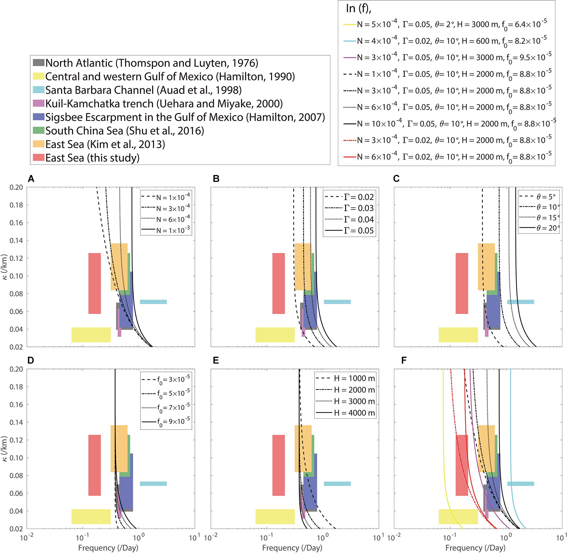
Figure 1. Dispersion relation (lines) of bottom-trapped TRWs from Eq. (1) for (A) varying buoyancy frequency (N) with constant bottom slope (Γ = 0.05), propagating orientation angle rotated from the isobath direction (θ = 10°), Coriolis parameter (f₀ = 8.8 × 10^{– 5} s^{– 1}), and depth level (H = 2000 m); (B) varying Γ with constant N (= 1 × 10^{– 3} s^{– 1}), θ (= 10°), f₀ (= 8.8 × 10^{– 5} s^{– 1}), and H (= 2000 m); (C) varying θ with constant N (= 1 × 10^{– 3} s^{– 1}), Γ (= 0.05), f₀ (= 8.8 × 10^{– 5} s^{– 1}), and H (= 2000 m); (D) varying f₀ with constant N (= 1 × 10^{– 3} s^{– 1}), Γ (= 0.05), θ (= 10°), and H (= 2000 m); (E) varying H with constant N (= 1 × 10^{– 3} s^{– 1}), Γ (= 0.05), θ (= 10°), and f₀ (= 8.8 × 10^{– 5} s^{– 1}); and (F) their combinations. Herein, ranges of wavenumbers (κ) and frequencies (ω) investigated in past and present studies are shaded with different colors, and references are presented.

The Ulleung Interplain Gap (UIG), located in the East Sea (Japan Sea), is the only deep passage (i.e., below 1500 m) connecting the Ulleung Basin (UB) in the southwestern area of the sea with the Japan Basin (JB) in the northern area (Figures 2A,B). Deep and abyssal currents observed below 1800 m from five moorings across the UIG for 16.5 months from November 2002 to April 2004 demonstrate an asymmetric structure of mean exchange flow with broad and weak equatorward inflow into the UB through the western UIG, and narrow and strong poleward outflow out of UB through the eastern UIG. The poleward outflow is named the Dokdo Abyssal Current (DAC) and exhibits a maximum recorded current speed of approximately 33.9 cm s^–1 (Chang et al., 2009). Strong variability in the upper ocean circulation revealing the meandering of the Tsushima Current, and mesoscale eddies in the UIG and UB have been reported (Mitchell et al., 2005; Teague et al., 2005; Xu et al., 2009). These currents may contribute to the generation of TRWs and result in the intraseasonal variability of the DAC. Indeed, the power spectra for deep flows in the UIG indicate high spectral energies over a period of 15–60 days, particularly near Dokdo, relevant to the steeply sloping bottom topography (Chang et al., 2009). Results consistent with spectral peaks of DAC variability at the relatively shorter periods of 10.7 and 21.3 day were reported from direct current observations of approximately five moorings from November 2002 to April 2004, supporting the notion of bottom-trapped TRWs with wavelengths of 50–80 km (Kim et al., 2013). However, the forcing mechanisms of DAC variability at a longer intraseasonal band (30–50 days) remain unknown, probably due the relatively short period of mooring observations, which makes resolving the current variability at the longer intraseasonal band difficult.

FIGURE 2

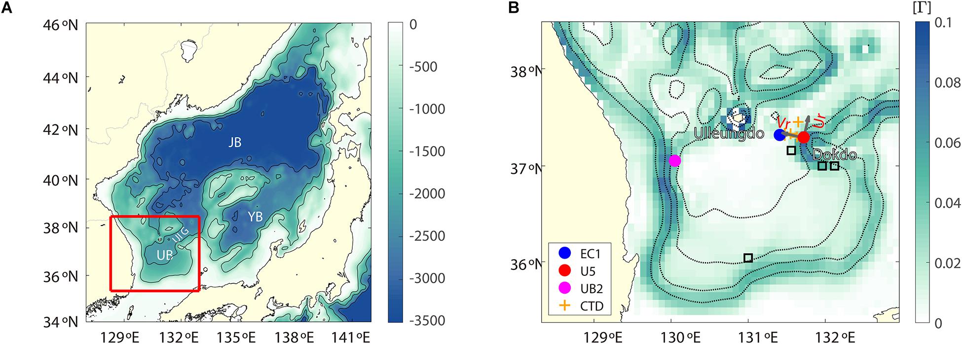
Figure 2. (A) Bottom topography (depth in color) in the East Sea. JB, YB, UB, and UIG denote the Japan Basin, Yamato Basin, Ulleung Basin, and Ulleung Interplain Gap, respectively. (B) Bottom slope in UB and UIG (area shown in red in panel A) with isobaths every 500 m. Locations of current-meter moorings (EC1, U5, and UB2) and conductivity–temperature–depth (CTD) casts are shown with circles and crosses, respectively. Four locations selected for calculating the TRW characteristics are indicated by colored squares (Cases 1–4). The along-slope (U_r) and down-slope (V_r) directions are marked with arrows in panel (B).

This study aims to characterize and address the bottom-trapped TRWs underlying the longer-period intraseasonal DAC variability from multi-year moored current-meter observations and HYbrid Coordinate Ocean Model (HYCOM) reanalysis, and to discuss the possible cause. The data and methods used are described in the next section. Section “Results” provides the TRW characteristic results derived from both observational and reanalysis data. The results are discussed in Section “Discussion” and concluded in section “Conclusion”.

Data and Theory

Data Source and Processing

We used long time-series data collected using three subsurface moorings, EC1, U5, and UB2, in the UB and UIG (Noh and Nam, 2018; Noh et al., 2020) (Figure 2B). At EC1, 14-year time-series moored current-meter data were collected at depths of approximately 1400 and 2200 m (with slightly varying sensor depths over deployments) from January 1999 to December 2012. Time-series acoustic Doppler current profiler data collected from the upper 300 m of the EC1 mooring from December 2002 to February 2004 were also used. Similar moored current-meter data were collected at U5 at depths of 1000 and 2000 m from November 2002 to May 2006, and at UB2 at depths of 1000 and 1600 m from May 2006 to February 2010. Aanderra rotary current-meters (RCMs) and Nortek Aquadopp current-meters were used to collect the moored current-meter data at sampling intervals of 30 or 60 min. The mooring locations, nominal depths of current meters, deployment periods of moorings, and basic statistics of the moored current-meter data are listed in Table 1. The speeds of the horizontal current shown in Table 1 are based on an uncertainty of an order of 0.01 cm s^–1, which is inversely proportional to the square root of the number of data used in averaging (Teague et al., 2005; Watts et al., 2013). The minimum current speed of an RCM is 1.1 cm s^–1, which is treated as a current stall, and a data gap of no longer than 5 h was filled by applying spline fits to the zonal and meridional currents (Teague et al., 2005). The moored current-meter data were vertically interpolated to estimate the zonal and meridional currents at the nominal depths.

TABLE 1

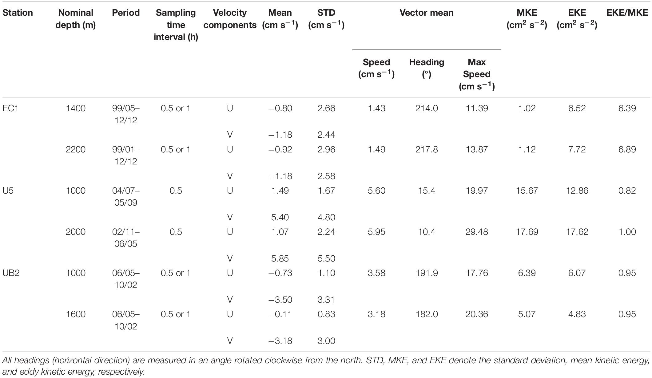
Table 1. Basic statistics of daily mean currents observed at EC1 for 1999 to 2012, U5 for 2002 to 2006, and UB2 for 2006 to 2010 along with sampling time interval of the current measurements.

The measured zonal (u) and meridional (v) currents were ensemble-averaged over 1 day. The ratio of $\text{EKE}=\left(\overline{u^{\prime 2}}+\overline{v^{\prime 2}}\right)/2$ to $\text{MKE}=\left(\overline{u^2}+\overline{v^2}\right)/2$ was calculated, where the zonal and meridional velocities (u,v) were decomposed into long-term mean $(\overline{u},\overline{v})$ and fluctuating components (u′,v′), that is, $u=\overline{u}+u^{\prime }$ and $v=\overline{v}+v^{\prime }$. The daily averaged u and v were bandpass-filtered to extract fluctuations at shorter (5–25 days) and longer (30–50 days) intraseasonal bands with cutoff periods of 5 and 25 days, and 30 and 50 days, respectively, using a second-order Butterworth filter. The two intraseasonal bands were based on spectral energies observed at U5 (rather than EC1), as reported in a previous study (e.g., Chang et al., 2009; Figure 3D). The variance-preserving spectrum of the current speed ($\sqrt{u^{\prime 2}+v^{\prime 2}}$) was calculated using Welch’s power spectrum methods (Welch, 1967) and Hamming windows with 50% overlap. In addition to the moored current-meter data, vertical profiles of temperature and salinity collected in the eastern UIG (near U5 and EC1) from six full-depth CTD casts in August 1995, March 1997, June 1999, September 2005, August 2008, and October 2012 were used to estimate the buoyancy frequency (Figure 2B).

FIGURE 3

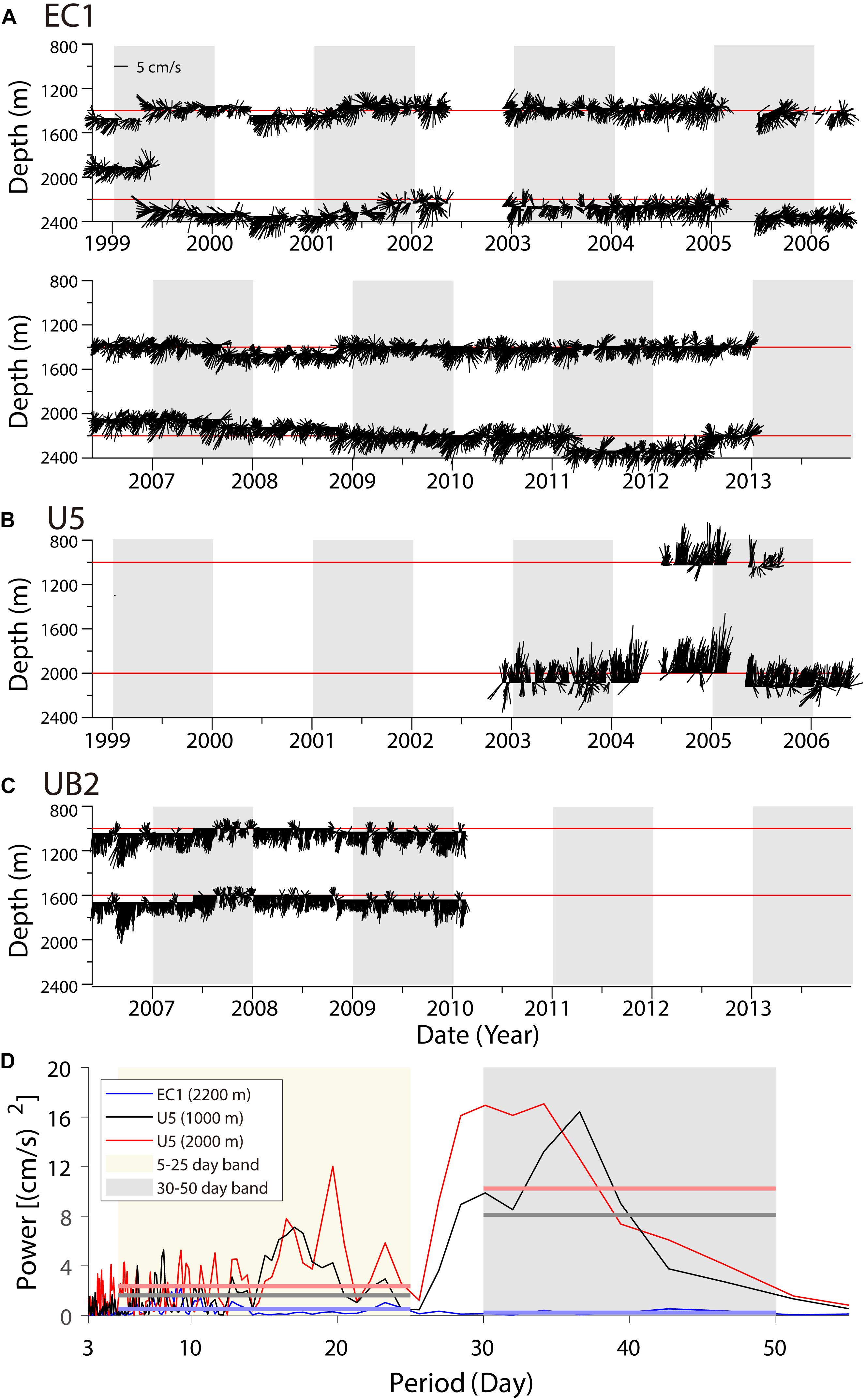
Figure 3. Time series of daily mean currents observed at (A) EC1, (B), U5, and (C) UB. The horizontal red bars denote the nominal depth. (D) Total kinetic energy spectra of EC1 (blue) and 1000 and 2000 m of U5 (black and red), in variance-preserving form of currents observed at 1000 m of U5 from July 2004 to September 2005. The horizontal bars refer to the mean spectral energy for shorter and longer intraseasonal bands (shaded).

The 20-year time-series data of daily u and v, water temperature, and salinity from October 1992 to December 2012 of HYCOM global 1/12° reanalysis data were used in this study. The horizontal resolution was 0.08°, and the vertically interpolated z-levels where the data were extracted were 100, 200, 300, 400, 500, 600, 700, 800, 900, 1000, 1250, 1500, and 2000 m. Although the data-assimilated HYCOM data may contain non-conservative momentum, vorticity, and mass source/sink elements, the results in the deep layer were not modified significantly with sparse or no available observational data in the region. Thus, the HYCOM data have been widely used to reveal intermediate and deep circulations in the region, which is consistent with observations reported elsewhere (Hogan and Hurlburt, 2006; Nam et al., 2016; Han et al., 2020). The HYCOM horizontal currents (u and v) were also bandpass-filtered with the same filters used to extract fluctuations at the two intraseasonal bands. Considering the bottom topography in the vicinity of U5, bandpass-filtered currents were decomposed into along-slope (U_r, 10° rotated clockwise from the north) and cross-slope (V_r) components. The bathymetry data used in the HYCOM dataset (GLBu0.08_07b) were used to estimate the along-isobath angle at scales of several tens to a few hundreds of kilometers (Figure 2B).

To supplement the observational and HYCOM data, the sea surface wind from the Modern-Era Retrospective analysis for Research and Applications, Version 2 (MERRA2), and the absolute sea surface height (SSH) from the Archiving, Validation, and Interpretation of Satellite Oceanographic data (AVISO) were used. The MERRA2 wind data were produced with a time interval of 6 h, and zonal and meridional resolutions of 0.2° for the atmospheric model. The AVISO SSH data, provided by the Copernicus Marine Environment Monitoring Service (CMEMS), were provided as daily gridded data from satellite altimetry missions, such as Jason-3 and Sentinel-3A, with a horizontal resolution of 0.25° × 0.25°.

Application of Bottom-Trapped TRW Theory

In the linear theory of bottom-trapped TRWs, the vertical structure of bottom-intensified wave motions is proportional to V = V₀cosh⁡(κNz/f₀), where V is the horizontal velocity component, κ is the horizontal wavenumber, and z is the water depth (Rhines, 1970). Neglecting the planetary beta, the dispersion relation of TRWs in a stratified ocean can be written as

$$\mathrm{\omega }=\mathrm{\Gamma }N\sin \mathrm{\theta }\coth (\mathrm{\kappa }NH/f_0),(1)$$

whereω, θ, N, H, f₀, and Γ are the wave frequency and orientation angle of the wavenumber vector from the downslope or the angle of the wave-propagating direction (direction of the group velocity vector) with respect to the isobath, buoyancy frequency, water depth, Coriolis parameter, and bottom slope, respectively. The ratio R of the kinetic energy associated with the TRWs between the two depths is expressed as:

$$R={(\cosh (\mathrm{\kappa }N{z}_1/f_0)/\cosh (\mathrm{\kappa }N{z}_2/f_0))}^2\text{for}{z}_1<z_2,(2)$$

where z₁ and z₂ are the two depth levels. Herein, R is estimated from the ratio of U_r spectra at the upper and lower layers for the intraseasonal band, and N and f₀ are fixed (6.8 × 10^–4 and 8.8 × 10^–5 s^–1, respectively) based on the time-mean vertical profiles of the HYCOM temperature and salinity near Dokdo. The wavenumber κ and thus the wavelength (λ = 2π/κ in km) and propagating speed (C = λ/T in km day^–1, where T is the period) are estimated from the ratio R using Eq. (2). The orientation angle (θ) is calculated in two ways. The first method uses the spectra of the along-slope and cross-slope currents (U_r and V_r) observed at 2000 m following the process described in Fofonoff (1969). Herein, the angle θ_e is obtained using the co-spectrum (S_uv) between U_r and V_r and the autospectrum (S_uu, S_vv) of U_r and V_r as follows:

$${\mathrm{\theta }}_{\text{e}}=\frac{1}{2}{\tan }^{-1}\frac{2S_{\text{uv}}}{S_{\text{uu}}-S_{\text{vv}}},(3)$$

The second method uses the theoretical dispersion relation (θ_t) with a constant bottom slope (Γ = 0.02 for the location of U5) and the buoyancy frequency N, as derived from Eq. (1):

$${\mathrm{\theta }}_{\text{t}}={\sin }^{-1}\left[\frac{2\mathrm{\pi }}{T\mathrm{\Gamma }N}\tanh (\frac{2\mathrm{\pi }}{f_0}\mathrm{\kappa }H)\right],(4)$$

where T is the period. The difference in the orientation angle between the two methods (θ_d = θ_e−θ_t) is used to examine the significance of the bottom-trapped TRW dynamics in the corresponding cases.

A small R, indicating the bottom intensification of intraseasonal oscillation, is a necessary condition for bottom-trapped TRWs. The eight small R cases selected in this study are listed in Tables 2, 3. Note that such bottom intensification is found in limited areas where the bottom-trapped TRW theory is applicable, mostly at the eastern side of the UIG and UB (shown in the next section). For the eight selected cases with Γ values ranging from 0 to 0.1, we tested the sensitivity of the theoretical orientation angle (θ_t) to the HYCOM buoyancy frequency N (7.0 ± 4.0 × 10^–4 s^–1), which is significantly overestimated compared with that of the CTD observation (3 × 10^–4 s^–1). The overestimation of the HYCOM stratification in the deep part of the region, accounting for most of the systematic bias in θ_d (systematically small θ_t compared with θ_e), is discussed with regard to the uncertainties of HYCOM-derived θ_t in section “Discussion”.

TABLE 2

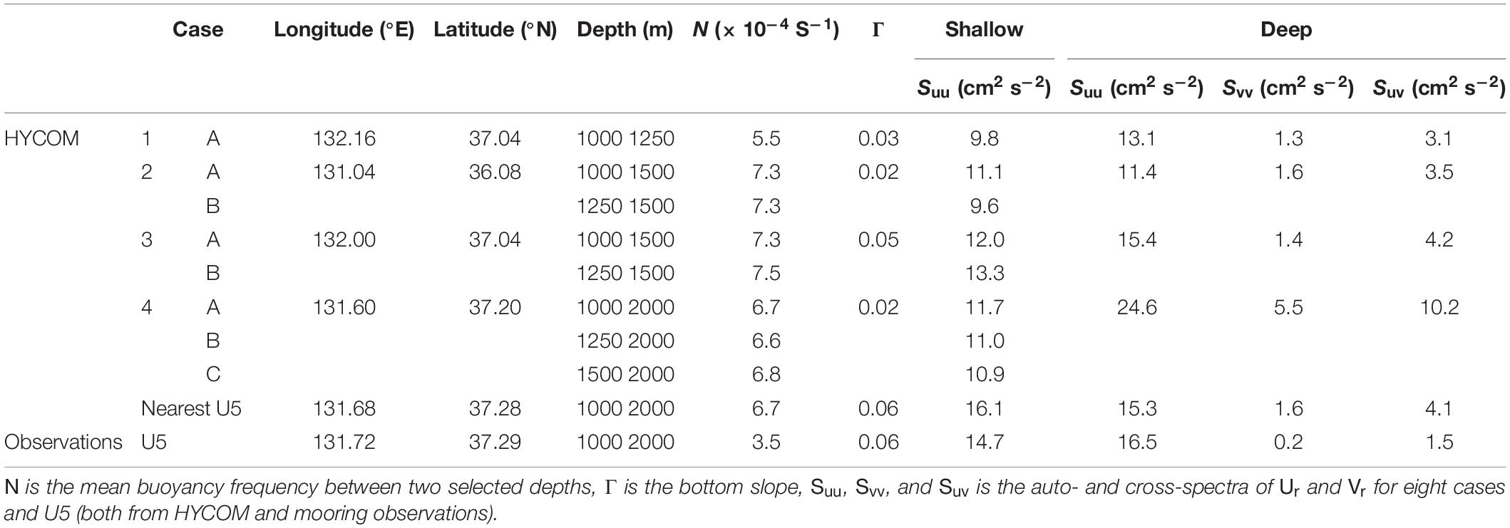
Table 2. Inputs of TRW parameters.

TABLE 3

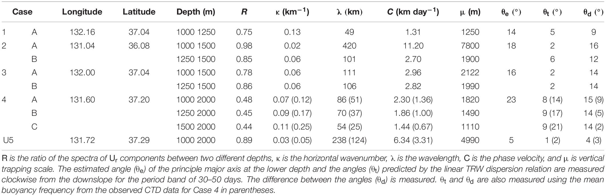
Table 3. TRW parameters for eight cases and observation (U5).

Results

Characteristics of Abyssal Circulation and Its Variability

Statistics on Abyssal Currents Observed in the UB and UIG

Weak southward and southwestward inflows from the JB into the UB via the UIG, with mean speeds of 1.43 and 1.49 cm s^–1, were observed at the 1400 and 2200 m levels, respectively, at EC1 in the center of the UIG. Here, an EKE 6–7-times larger than the MKE indicates significant temporal variability (Figures 3A, 4A and Table 1). The kinetic energy spectra of abyssal currents observed at 2200 m indicate distinct, significant variances of 0.53 and 0.23 cm² s^–2 at shorter and longer intraseasonal bands (5–25 and 30–50 days, respectively) at U5; however, the separation was not distinct at EC1 (Figure 3D). The two intraseasonal bands defined previously were based on spectral energies observed at U5 rather than EC1 (Chang et al., 2009).

FIGURE 4

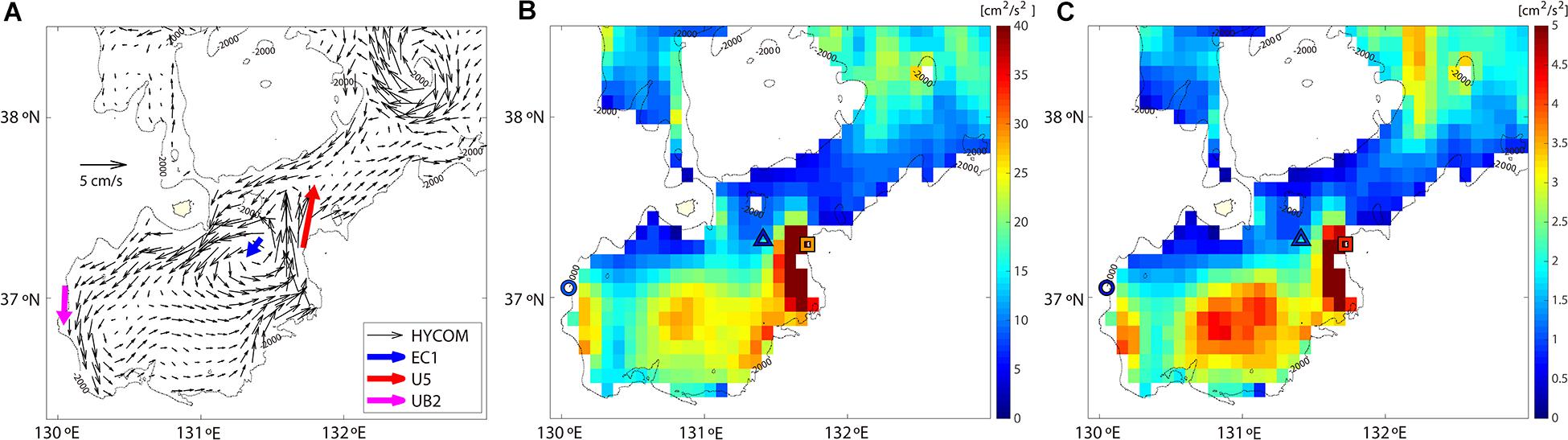
Figure 4. Statistics of deep currents reproduced by HYCOM reanalysis data and moored data. (A) Mean velocity field using HYCOM data and moored data at EC1, U5, and UB2 (black, blue, red, and purple arrows, respectively), and variance of v currents for (B) unfiltered case and (C) longer intraseasonal band. In panels (B,C), the colors of the symbols for EC1 (triangle), U5 (square), and UB2 (circle) denote the variance of the observed v currents with the same scale shown in the right color bar.

Unlike EC1, relatively strong northward flows were observed at U5, with mean speeds of 5.60 cm s^–1 at 1000 m and 5.95 cm s^–1 at 2000 m. Southward flows were observed at UB2 with mean speeds of 3.58 cm s^–1 at 1000 m and 3.18 cm s^–1 at 1600 m (Figures 3B,C, 4A and Table 1). Although U5 and EC1 are adjacent to each other, the maximum speed of abyssal currents at U5 was 29.48 cm s^–1, which is twice that at EC1. The difference between maximum current speeds at U5 and EC1 is due to the asymmetric flow structure across the UIG, with a wider and weaker inflow into the UB located in the western UIG, and a narrower and stronger outflow into the JB located in the eastern UIG, which is consistent with the findings of previous studies (Chang et al., 2009) and confirmed from HYCOM (Figure 4A). The relatively strong northward abyssal currents at U5 reaffirm the DAC in the eastern UIG.

Despite the lower ratios (∼1) at U5 and UB2 between EKE and MKE than those at EC1, temporal variability is stronger at U5 and UB2, yielding variances at 2000 m of 1.62 and 8.11 cm² s^–2, respectively, in the kinetic energy spectra of abyssal currents. These variances are several times higher than those at EC1 at shorter and longer intraseasonal bands (5–25 and 30–50 days, respectively; Figures 3A–D, 4A, and Table 1). The spectral variances of kinetic energy at 1000 m for U5 are 2.35 and 10.24 cm² s^–2 at shorter and longer intraseasonal bands, respectively. These values are lower than the spectral variances at 2000 m at U5, indicating bottom intensification. The mean and fluctuating currents (particularly at the longer intraseasonal band) are intensified at U5 on the eastern side near Dokdo, indicating eastward intensification.

Comparison of Observed and Reanalyzed Abyssal Currents

The HYCOM deep currents in the UB and UIG show cyclonic circulation along the 2000 m isobath, which consists of a weak southward inflow to the UB in the western UB and UIG, a weak eastward flow in the interior and southern UB, a strong northward outflow from the UB in the eastern UB and UIG, and smaller cyclonic circulation near EC1 (Figure 4A). The cyclonic deep and abyssal circulation are consistent with the observations at EC1, U5, and UB2. The spatial distribution of v variance at the longer intraseasonal band shows severe variability in the eastern UIG and UB, which accounts for most of the v variance (Figures 4B,C). The eastward intensification of v is also consistent with the observations in EC1, U5, and UB (Figures 4B,C and Table 1).

The spatial distribution of the correlation between the reanalyzed and observed v at EC1 and U5 in the non-filtered case, and the shorter and longer intraseasonal bands, is shown in Figure 5. The correlation of the non-filtered v current shows the tendency for asymmetric flow between the eastern and western UIG and UB. Although there was no significant correlation in the shorter intraseasonal band at EC1 and U5, marginally significant correlations with the longer intraseasonal band at U5 were found in large areas of the UB and UIG. However, as EC1 is located in the central UIG, which reveals a relatively clear tendency of asymmetric flow in the longer intraseasonal band, it represents the western UIG.

FIGURE 5

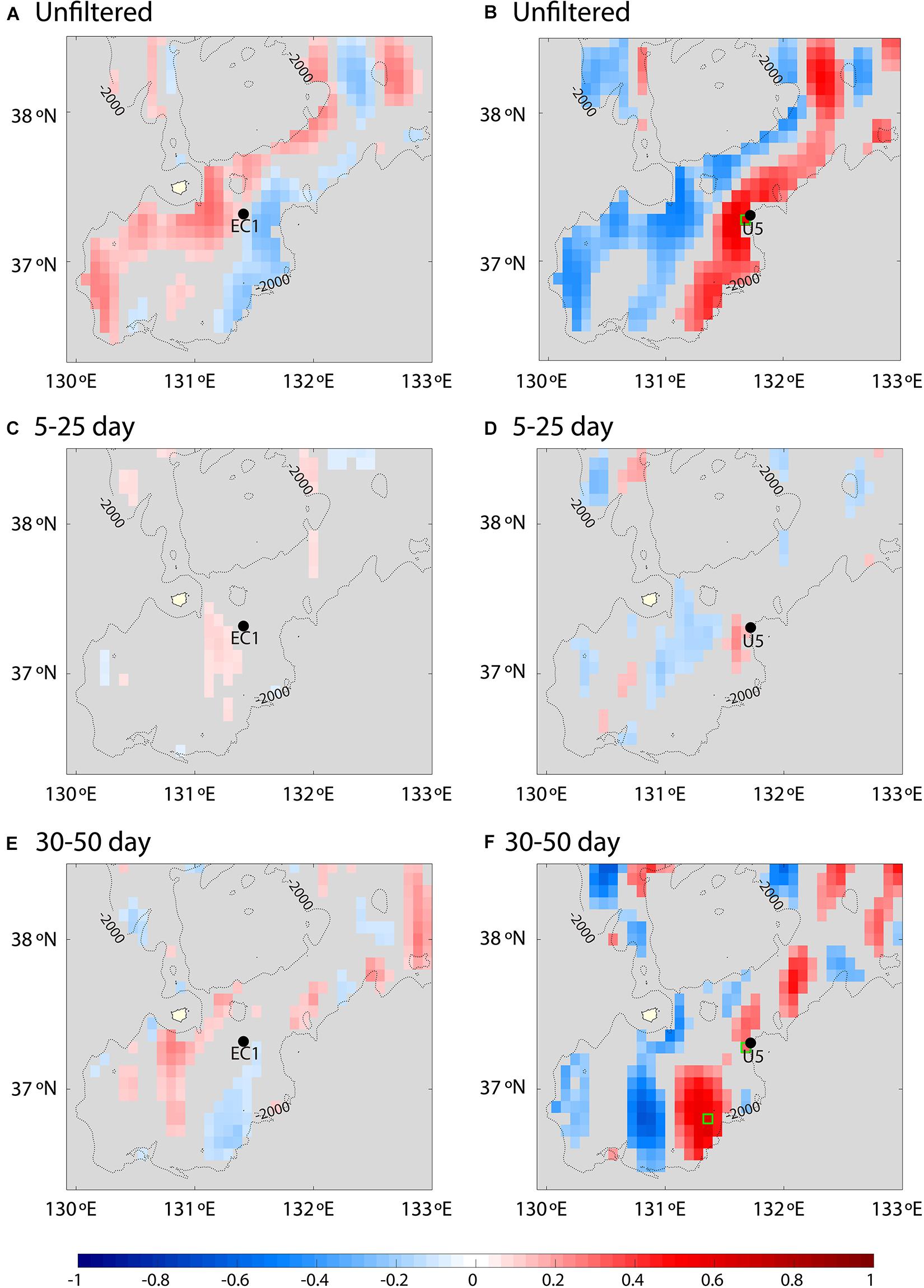
Figure 5. Correlation (values below 95% confidence level are discarded) between modeled (HYCOM) and observed v currents for EC1 (left) and U5 (right) at 2000 m for (A,B) the whole period band, (C,D) shorter intraseasonal bands, and (E,F) longer intraseasonal bands. Grids selected for comparison of observed and modeled abyssal currents are marked by green squares.

The marginally significant correlations in the longer intraseasonal band v observed at U5 were confirmed in the time series plots (Figure 6). At U5, the reanalyzed v at 2000 m is not highly correlated with the observation at U5 for the longer intraseasonal band, although it is statistically significant (correlation coefficient: ∼0.30; Figure 6C). A better correlation (∼0.57) with the observation is found in the southeastern UB (green square in Figure 5F), where the reanalyzed and observed v at 2000 m are generally consistent in both phase and amplitude (Figure 6D). The reanalyzed and observed v are not only marginally correlated but also consistent in terms of amplitude and vertical propagation. Vertical phase propagation was not significant for both observations and reanalyzed v except for the upper depths, particularly between 1000 and 2000 m (Figures 6B,E,F). At U5, the lagged cross-correlation reached its maximum (0.79) at zero lag for reanalysis v at 1000 and 2000 m.

FIGURE 6

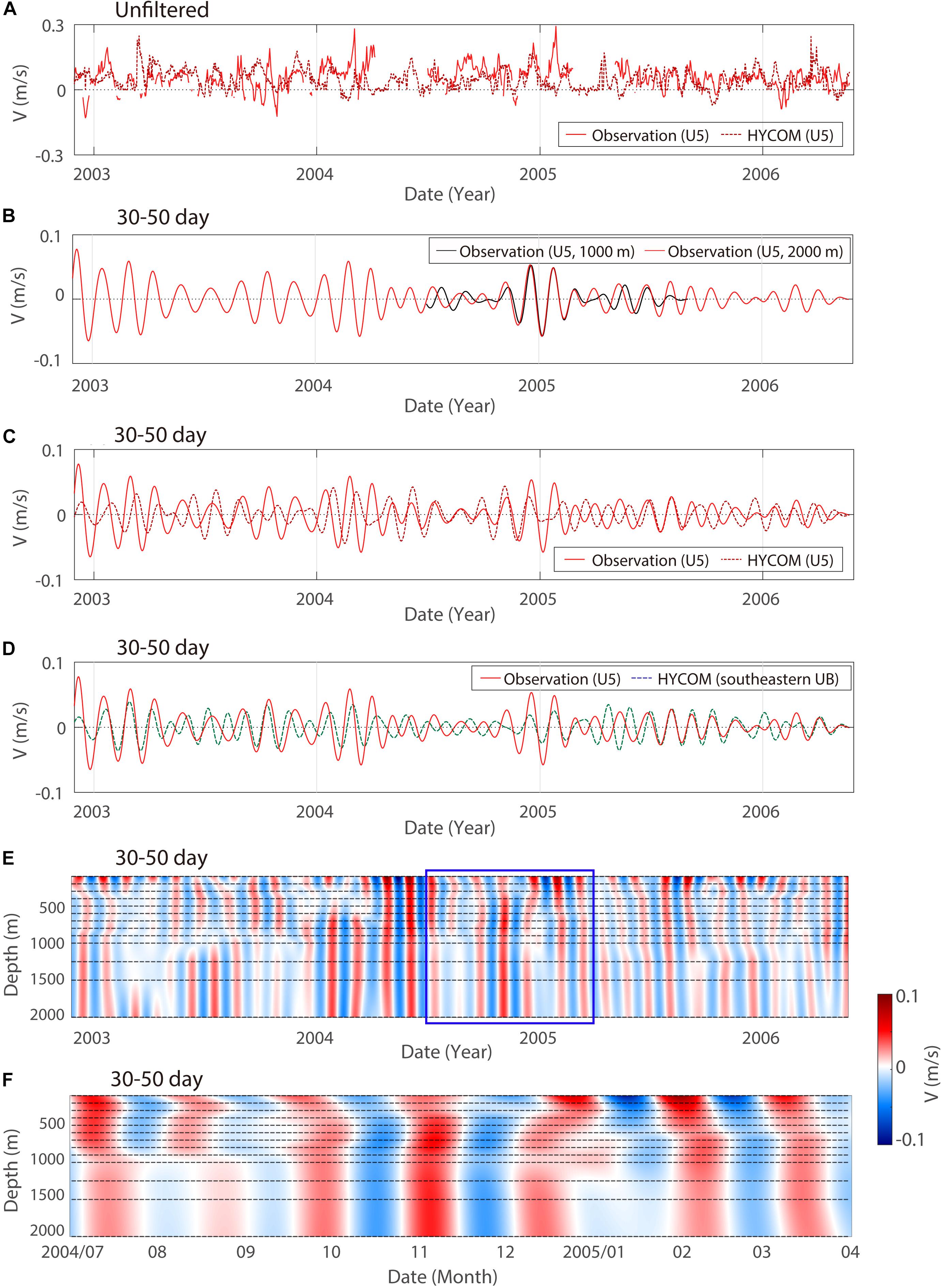
Figure 6. Time series of modeled (dashed) and observed (solid) v currents at 2000 m of the locations of (A,C) U5 and (D) southeastern UB (green squares in Figure 5) for the (A) unfiltered and (C,D) longer intraseasonal band. Those of v currents observed at 1000 m (black) and 2000 m (red) of the location of U5 are compared in panel (B). Time-depth contours of modeled v currents are shown for longer intraseasonal band at U5 for (E) total period and (F) period from July 2004 to April 2005. The HYCOM depth levels are denoted by black dotted horizontal lines in panels (E,F).

Characteristics of Intraseasonal Abyssal Current Variability and TRWs

Spatially Coherent Abyssal Current Variability in the Intraseasonal Band

The correlation maps of reanalyzed v show wave-like spatially coherent patterns in the western, central (corresponding to EC1), and eastern (corresponding to U5) UIG v at 2000 m (Figures 7A–C). The results show an opposing sign between the western and eastern sides of the UIG and UB, implying that waves were constrained by basin geometry; for example, the normal mode. The horizontal width of the coherent pattern with a positive correlation is wide at the western and narrow at the eastern UIG and UB, consistent with the asymmetrical characteristics of the observed and reanalyzed mean currents ($\overline{u}$, $\overline{v}$). The wave-like patterns with a phase change every ∼80 km indicate wavelengths comparable to the scale in this region.

FIGURE 7

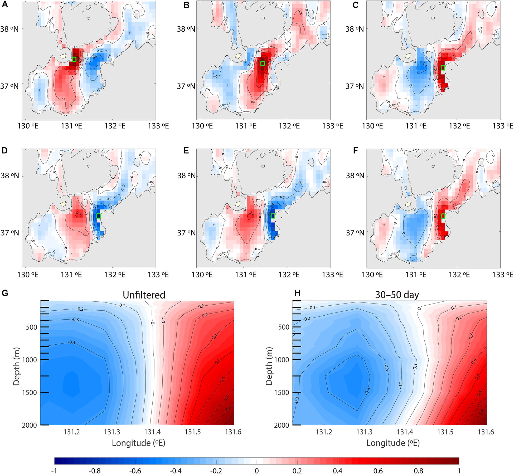
Figure 7. Correlation map, with no lag, of HYCOM deep currents with those in (A) the western UIG, (B) central UIG (nearest to EC1), and (C) eastern UIG (nearest to U5), for the longer intraseasonal band with contours every 0.2 from –1.0 to 1.0. A lagged correlation map in the eastern UIG (D) before 20 days, (E) after 20 days, and (F) after 5 days. Grids of referenced HYCOM currents are marked by green squares. The correlation map, with no lag, of HYCOM meridional currents with those in deep eastern UIG (U5) are shown across the vertical UIG section (G) without and (H) with band-pass filtering (longer intraseasonal band). The HYCOM depth levels are denoted by left axis ticks in panels (G,H).

Regarding the phase change, a nearly identical spatial pattern of the correlation map v was obtained with time lags before and after 20 days (half the longer intraseasonal band v). Phase changes from positive to negative and back again were observed (Figures 7D,E), although no significant change was observed after a 5-day lag (Figures 7C,F). Cross-sectional correlation maps support both the eastward and bottom intensification of the longer intraseasonal DAC oscillations, yielding e-folding decorrelation length scales of ∼11 km in the cross-slope and ∼1400 m in the vertical direction (Figures 7G,H). The ratio between the vertical and cross-slope scales, 0.13 (= 1400/11000), which is more than double the bottom slope at U5 (0.06, Table 2), is discussed in the next section. Such high ratio supports even strongly bottom-trapped or first baroclinic structures vertically (note that zero-crossing depth corresponds to the thermocline at approximately 100 m). These dominant correlation patterns, along with the eastward intensification of the intraseasonal current oscillations, raise the possibility of bottom-trapped TRW or the first mode of baroclinic Rossby waves, as presented in the next section.

Characteristics of Bottom-Trapped TRWs

Bottom intensification with a stronger HYCOM current at lower depths (R < 1) is found at the eastern UB and UIG along the 1250, 1500, and 2000 m isobaths, particularly near Dokdo (Figure 8). Although there are a few grids beyond the eastern side where R is less than 1.00 (e.g., in the southern UB and western interior UB), the minimum value of R is 0.91. This is significantly higher than the R values in the eastern DAC near Dokdo. Thus, the bottom-trapped TRW theory is primarily applicable for areas limited to the eastern side of the UIG and UB, where the minimum value of R is 0.45 (Figures 8D–F). The bottom and eastward intensification of the longer intraseasonal current variability is consistent with the observed characteristics presented in the previous section, and is characterized in association with bottom-trapped TRWs.

FIGURE 8

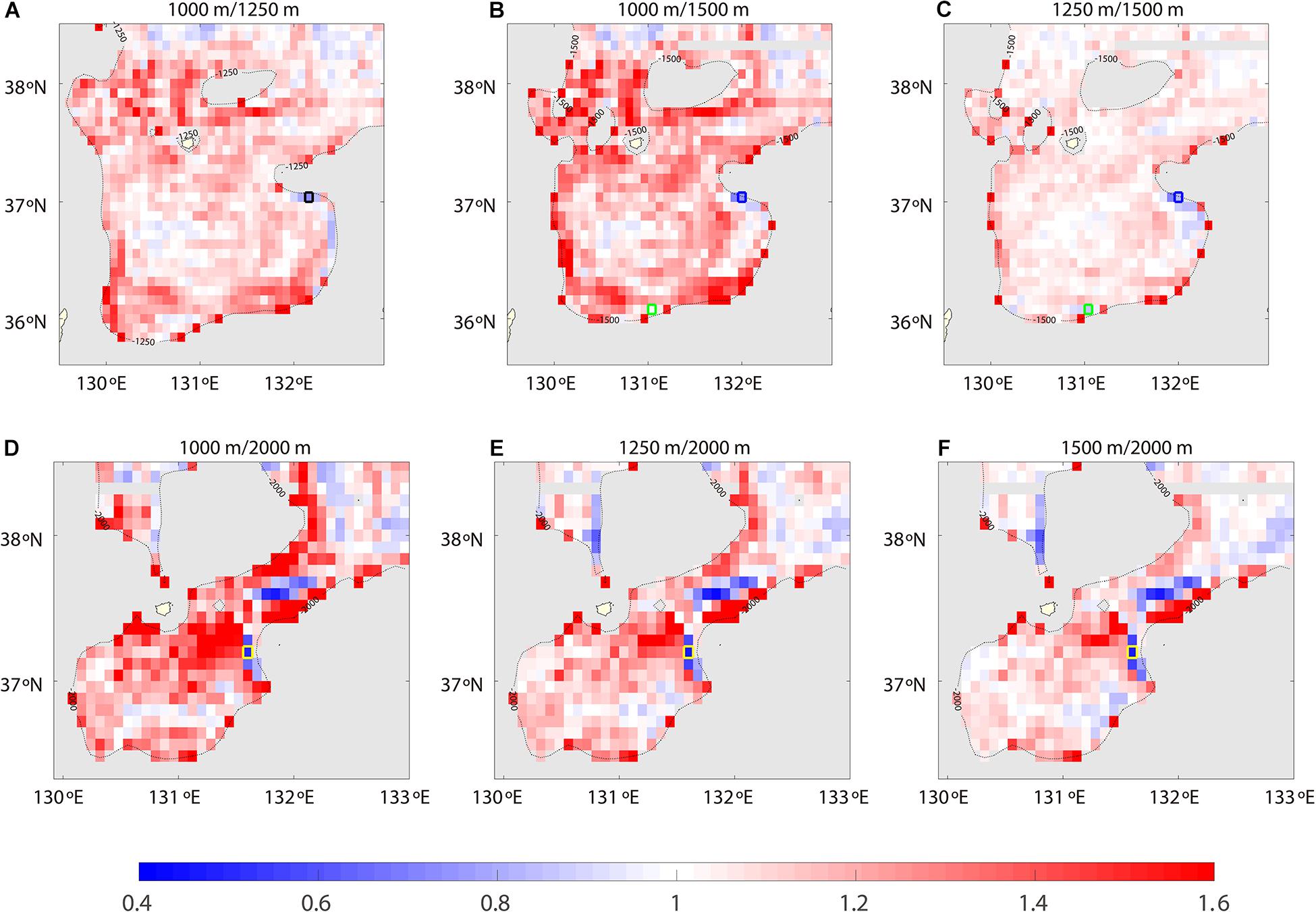
Figure 8. Spatial distribution of R for the longer intraseasonal band between two different depths for (A) 1000 and 1250 m, (B) 1000 and 1500 m, (C) 1250 and 1500 m, (D) 1000 and 2000 m, (E) 1250 and 2000 m, and (F) 1500 and 2000 m. Grids where R is below 1 indicate bottom intensification and the four selected cases where the bottom intensification is distinct are marked by squares.

The horizontal wavenumber, wavelength, phase speed, orientation angle of the wavenumber vector (from the two methods), and vertical trapping scale listed in Table 3 provide the characteristics of bottom-trapped TRWs that explain the observed abyssal current variability in the longer intraseasonal band. A small (<16°) difference in the orientation angle exists between the two methods (θ_d) for the eight cases from HYCOM reanalysis and observation at U5 (Table 3). The observational results, in comparison to the corresponding HYCOM case (Case 4A), show weaker bottom intensification (higher R), resulting in longer wavelength, larger vertical trapping scale, lower propagating speed, and smaller θ_e. The HYCOM results yield wavelengths of 54–86 km and a propagating speed of 1.44–2.30 km day^–1 for Case 4, in which the bottom intensification is the strongest. The vertical trapping scales of the HYCOM results are 1110–1820 m, which is consistent with the vertical structure (not shown) for Case 4. Meanwhile, θ_d ranges from 9° to 16° over all HYCOM cases, which is systematically biased to a positive value (i.e., a systematically small θ_t compared to θ_e), as discussed in the next section.

Discussion

The results of the orientation angle derived from the theoretical dispersion relation (θ_t) of Eq. (4) may be sensitive to the bottom slope (Γ) and buoyancy frequency (N). The sensitivity tests result in a range of θ_t typically less than 10° for the given range of the bottom slope in the case area (shaded area in Figure 9), and the buoyancy frequency obtained from the HYCOM stratification (±1 standard deviation from the mean, lines in Figure 9). Such a robust theoretical orientation angle of bottom-trapped TRWs (θ_t) cannot explain why θ_t is systematically smaller than the orientation angle derived from the spectra of U_r and V_r (θ_e) using Eq. (3), which is consistent with the observed currents. Interestingly, when compared with the CTD data (N = ∼3 × 10^–4 s^–1), the HYCOM reanalysis overestimates the mean buoyancy frequency (N) in the deep UB and UIG by ∼4 × 10^–4 s^–1 (Figure 10), which results in an overestimation of θ_t and θ_d for Case 4 of ∼6°–12° (Table 3). The parameters of TRWs using the observed N (Table 3 in parentheses and the blue line in Figure 9D) show a decrease in wavelength from 54 to 25 km and in propagating speed from 1.44 to 0.67 km day^–1 for Case 4c. The θ_t increases from 9° to 21° with the observed N, significantly decreasing θ_d from 14° to 2°. The resultant θ_d is thus within the range of uncertainty of HYCOM reanalysis data, supporting the significance of bottom-trapped TRWs in accordance with the observed stratification at the eastern side of UIG and UB.

FIGURE 9

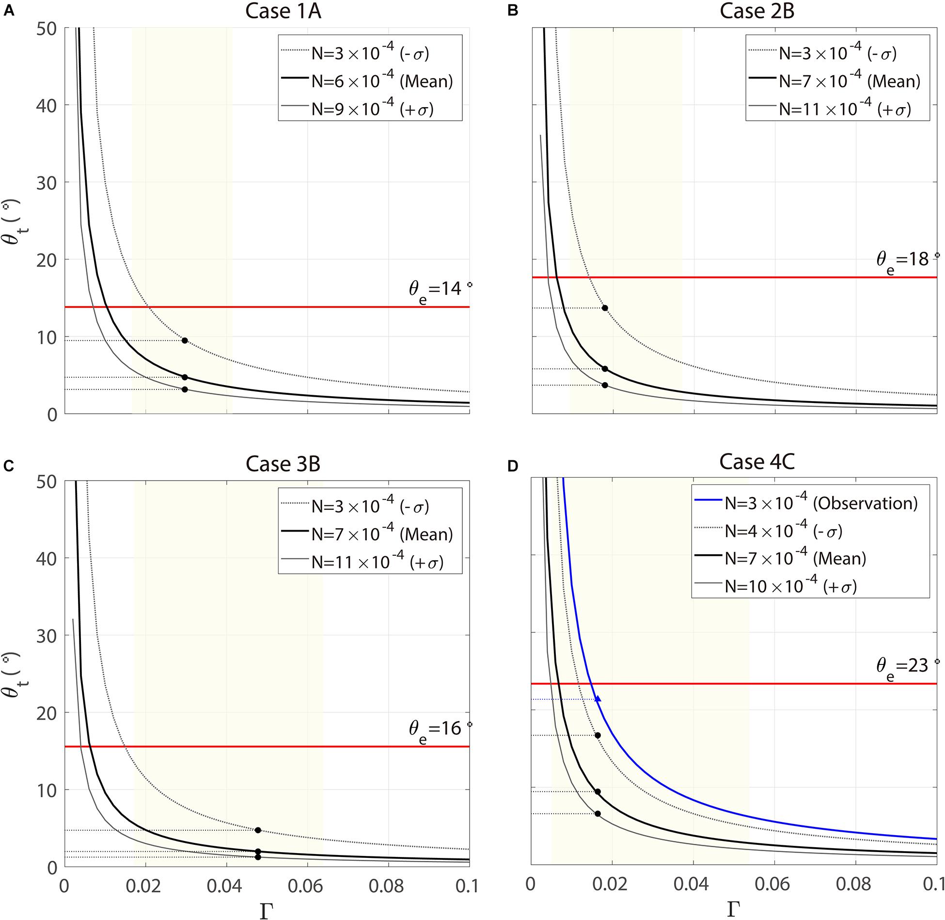
Figure 9. Sensitivity analysis for TRW parameters with bottom slope and buoyancy frequency for (A) Case 1A, (B) Case 2B, (C) Case 3B, and (D) Case 4C. The horizontal red line denotes the estimated angle (θ_e), and black dots denote the corresponding slope of the predicted angles of that grid for the mean and one standard deviation above and below the mean buoyancy frequency from the HYCOM reanalysis data (gray, gray dashed, and black lines, respectively). The adjacent slope range to each grid is shown for the yellow-shaded areas. For Case 4C, the blue line denotes the mean buoyancy frequency from the observed CTD data.

FIGURE 10

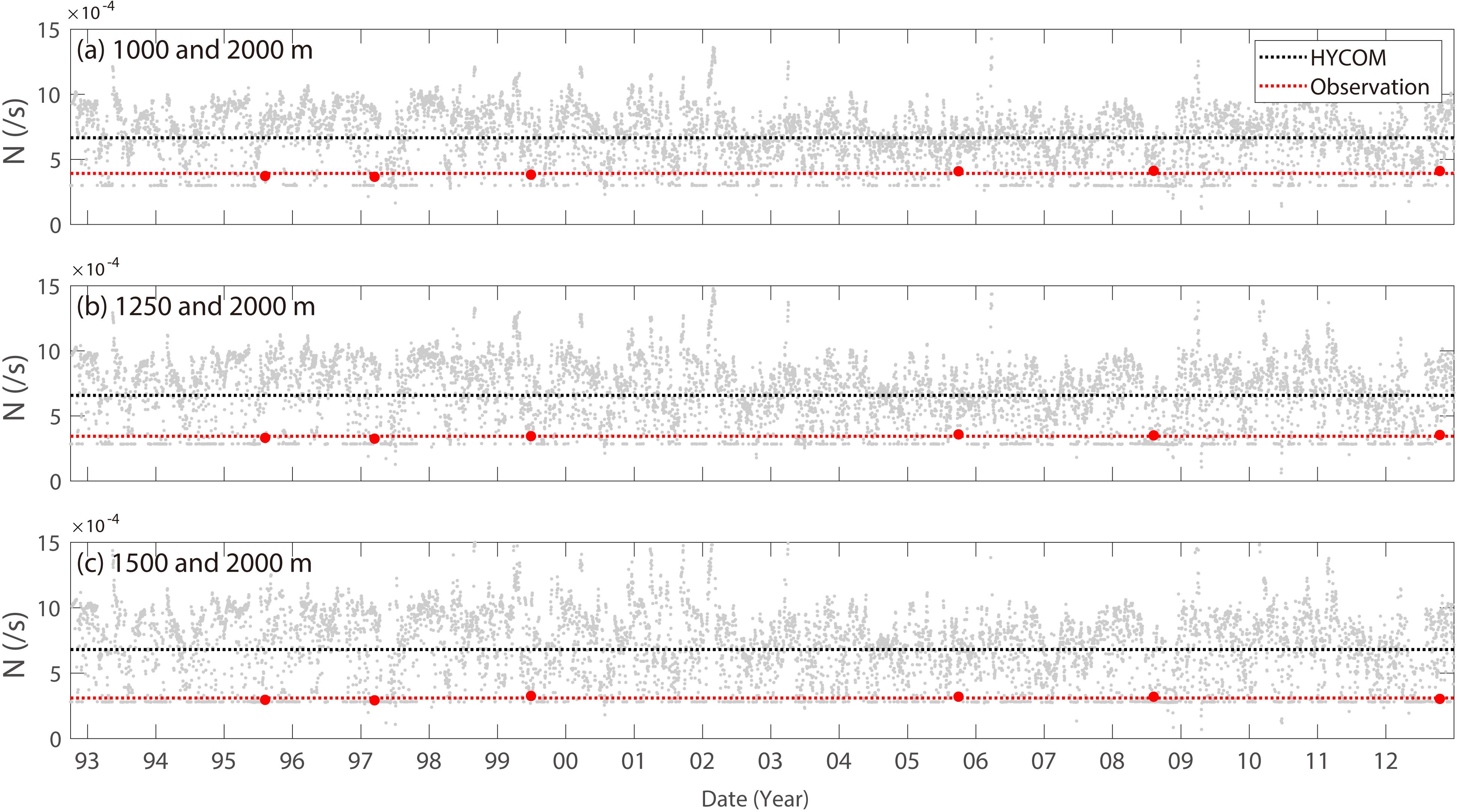
Figure 10. Time series of buoyancy frequency between two depths using HYCOM data for Case 4 (gray dots). The CTD data taken near the grid in Case 4 are marked by red dots. The horizontal bars refer to the mean buoyancy frequency of the HYCOM data (black line) and CTD data (red line) at (a) 1000 and 2000 m, (b) 1250 and 2000 m, and (c) 1500 and 2000 m.

The primary sources of TRW energy have been suggested by previous studies (Hamilton, 1990, 2007, 2009; Pickard, 1995; Auad et al., 1998; Oey et al., 2009; Oey, 2008; Shu et al., 2016). Energetic motions, such as mesoscale eddies and the meandering of the Tsushima Current, may play a role in the intraseasonal current variability in the upper layer of the southwestern East Sea, including the UB and UIG (Mitchell et al., 2005; Teague et al., 2005; Xu et al., 2009). In particular, Kim et al. (2013) reported that TRWs with periods of 10.7 and 21.3 day are generated from upper warm events (passing by the anticyclonic eddy), whereas those with periods of 40 days are less correlated with the upper warm events. The enhanced current oscillations observed (U5) and reanalyzed at the upper and lower depth levels at the longer intraseasonal band are significantly correlated with each other but less correlated with satellite altimeter-derived surface geostrophic current (not shown). Instead, these oscillations tend to intensify in winter when the longer intraseasonal band fluctuation of sea surface wind is also significant. The cause of the bottom-trapped TRWs responsible for the longer intraseasonal current variability is still obscure and needs further study.

In this study, the bottom-trapped TRW theory was applied to examine the bottom and eastward-intensified, longer intraseasonal variability in the abyssal current focusing on the eastern side of the UB and UIG. The relative importance of bottom trapping (baroclinic mode) vs. geostrophic motion (barotropic mode) can be easily evaluated with the index of ΓN/f₀ (Rhines, 1970), which is consistent with the stratification parameter (Wang and Mooers, 1976). For a given stratification and Coriolis parameter, a strong bottom trapping or baroclinic mode is dominant only when the slope is steep enough to bring the index close to or higher than the unity (high stratification parameter); otherwise, the motion is almost geostrophic or barotropic (low stratification parameter), as the index is much less than the unity with a gentle slope. For most of the UB and UIG areas, ΓN/f₀=∼0.1 or <1, and ΓN/f₀=∼1 or > 1 only at limited locations on the eastern sides (Figure 8), indicating that the barotropic mode of TRWs significantly contributes to the abyssal current variability in these areas. However, in the limited area of the steeply sloped eastern side of the UB and UIG (e.g., U5), ΓN/f₀ becomes much higher than the unity, with a high ratio between the vertical and cross-slope decorrelation scales at U5 (Figure 7H) indicating the dominant bottom-trapped or first baroclinic mode. Meanwhile, as the UB can be regarded as a closed basin, the existence of a normal mode is possible (Pedlosky, 1987). The horizontal wavelength estimated herein based on bottom-trapped TRW theory (49–111 km) is consistent with that of the first normal mode baroclinic Rossby waves for an equivalent depth and eigenvalue imposed by the closed basin scale on the order of 100 km. The estimation is also reasonable based on the correlation maps shown in Figures 7A–F. Further studies on the modes of Rossby waves besides the bottom-trapped mode (barotropic and baroclinic modes) are needed to fully understand the intraseasonal variability in the abyssal and upper currents in the region.

In other regions where bottom-trapped TRWs dominate the intraseasonal deep or abyssal current variability (Figure 1), the dominant wave period is shorter than 30 days, except in the central and western parts of the Gulf of Mexico where dominant periods range from 20 to 100 days (Thompson and Luyten, 1976; Hamilton, 1990, 2007; Auad et al., 1998; Shu et al., 2016). One noticeable characteristic of UB and UIG is that their observed N (from CTD observations) is one order of magnitude smaller than that in the other regions. This increases the wavenumber from 0.05 to 0.1 km^–1 and decreases the wavelength from 130 to 50 km, as shown by R = 0.5 in Eq. (2). Despite the small N, however, no significant differences in the wavenumber of bottom-trapped TRWs and propagating speed (which are one order of magnitude smaller because of the relatively longer intraseasonal band) are shown from those in the other regions because the small N is compensated by Γ and R, which shape the typical characteristics of TRWs in the UB and UIG.

Conclusion

To characterize and address the bottom-trapped TRWs underlying the longer-period intraseasonal variability of abyssal currents in the southwest East Sea (time scale of 30–50 days), multi-year moored current observations and HYCOM reanalysis were examined. The reanalysis data in the UB and UIG showed significant correlations (maximum 0.57 in the northeast UB) of the observed abyssal current variability in the intraseasonal band in the eastern UIG (U5), but with opposite signs: positive in the eastern region and negative in the western regions. The bottom-trapped TRWs in the eastern UB and UIG were responsible for the bottom-intensified current variability, based on the wavelength ranging from 49 to 111 km, propagating speed ranging from 1.3 to 3.0 km day^–1, a vertical trapping scale ranging from 1100 to 2100 m, and the orientation angle of the group velocity from the isobath direction ranging from 2° to 23°, except for one case (Case 2A). The orientation angle was estimated using two methods: one from the along-slope and cross-slope currents (U_r and V_r) of the observed and modeled deep intraseasonal current fluctuations (θ_e), and the other from the theoretical dispersion relation of the bottom-trapped TRWs for a given buoyancy frequency and bottom slope (θ_t). The two orientation angles ranged from 14° to 23° and from 2° to 9°, respectively, yielding a relatively small (16° at the most) but positively biased difference (θ_d), in which the latter was mostly explained by the overestimation of stratification in the reanalyzed data. The results were robust (insensitive) to a reasonable range of buoyancy frequency and bottom slope in the region, suggesting that the bottom-trapped TRWs were responsible for the energetic abyssal circulation at the limited location of the eastern UB and UIG, where the bottom slope is sufficiently steep.

This study supports the important role of bottom-trapped TRWs in shaping the abyssal current variability in the eastern UIG and UB, strongly implying the exchange of water and materials between two deep basins in the East Sea: the UB in the southwest and the JB in the north. Abyssal currents are energetic as bottom-trapped TRWs propagate at a shallow depth, Dokdo, to the right (Figure 11). With the abyssal current variability at shorter intraseasonal periods (10–20 days) found previously, the TRWs are responsible for energetic longer intraseasonal band variabilities in the abyssal circulations in the areas of steep slope in the eastern UIG and UB. More observations are needed to further verify the HYCOM results and improve our understanding of deep, abyssal, and overturning circulation in these areas, including the barotropic and other baroclinic modes of TRWs with complex topography, as in the southwestern East Sea.

FIGURE 11

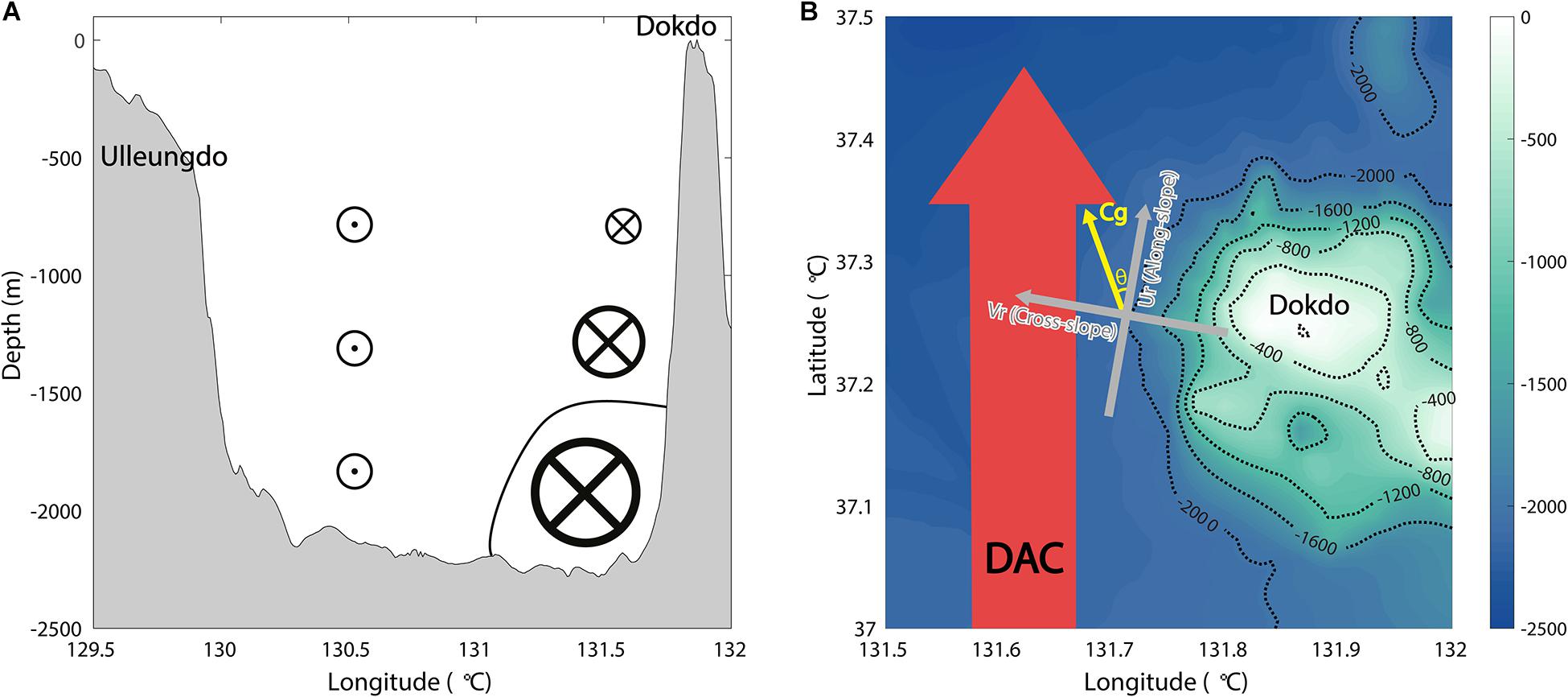
Figure 11. Schematic of the TRWs. (A) Side view at 37.25°N between Ulleungdo and Dokdo. (B) Detailed bathymetry near Dokdo with isobaths every 400 m. The angle (θ) indicates the direction of the wavenumber vector.

Data Availability Statement

Publicly available datasets were analyzed in this study. This data can be found here: http://doi.org/10.17882/72344; http://doi.org/10.17882/58134; http://hycom.org; http://www.marine.copernicus.

Author Contributions

All authors contributed to the article in multiple ways. SHN and JS designed the study. JS and SN performed the data processing and analysis. SHN, JS, and SN performed the synthesis and overall coordination. SHN, JS, and SN contributed to writing through discussion. SHN and SN contributed to revising through review.

Funding

This research was a part of the project titled ‘Deep Water Circulation and Material Cycling in the East Sea,’ funded by the Ministry of Oceans and Fisheries, South Korea. This work was partly supported by the Institute Civil Military Technology Cooperation, South Korea (18-SN-RB-01).

Conflict of Interest

The authors declare that the research was conducted in the absence of any commercial or financial relationships that could be construed as a potential conflict of interest.

Acknowledgments

We would like to thank Editage for English language editing and reviewers for their constructive comments, and Yun-Bae Kim and Kyung-Il Chang for providing current and hydrographic data.

References

Auad, G., Hendershott, M. C., and Winant, C. D. (1998). Wind-induced currents and bottom-trapped waves in the Santa Barbara Channel. J. Phys. Oceanogr. 28, 85–102. doi: 10.1175/1520-04851998028<0085:WICABT<2.0.CO;2

CrossRef Full Text | Google Scholar

Chang, K. I., Kim, K., Kim, Y. B., Teague, W. J., Lee, J. C., and Lee, J. H. (2009). Deep flow and transport through the Ulleung Interplain Gap in the southwestern East/Japan Sea. Deep Sea Res. Part I Oceanogr. Res. Pap. 56, 61–72. doi: 10.1016/j.dsr.2008.07.015

CrossRef Full Text | Google Scholar

Fofonoff, N. P. (1969). Spectral characteristics of internal waves in the ocean. Deep Sea Res. 16, 59–71.

Google Scholar

Hamilton, P. (1990). Deep currents in the Gulf of Mexico. J. Phys. Oceanogr. 20, 1087–1104. doi: 10.1175/1520-04851990020<1087:DCITGO<2.0.CO;2

CrossRef Full Text | Google Scholar

Hamilton, P. (2007). Deep-current variability near the Sigsbee Escarpment in the Gulf of Mexico. J. Phys. Oceanogr. 37, 708–726. doi: 10.1175/JPO2998.1

CrossRef Full Text | Google Scholar

Hamilton, P. (2009). Topographic rossby waves in the Gulf of Mexico. Prog. Oceanogr. 82, 1–31. doi: 10.1016/j.pocean.2009.04.019

CrossRef Full Text | Google Scholar

Hamilton, P., and Lugo-Fernandez, A. (2001). Observations of high speed deep currents in the northern Gulf of Mexico. Geophys. Res. Lett. 28, 2867–2870.

Google Scholar

Han, M. H., Cho, Y.-K., Kang, H.-W., and Nam, S. (2020). Decadal changes in meridional overturning circulation in the East Sea (Sea of Japan). J. Phys. Oceanogr. 50, 1773–1791. doi: 10.1175/JPO-D-19-0248.1

CrossRef Full Text | Google Scholar

Hogan, P. J., and Hurlburt, H. E. (2006). Why do intrathermocline eddies form in the Japan/East Sea? Model. Perspect. Oceanogr. 19, 134–143.

Google Scholar

Kim, Y. B., Chang, K. I., Park, J. H., and Park, J. J. (2013). Variability of the dokdo abyssal current observed in the Ulleung Interplain Gap of the East/Japan Sea. Acta Oceanol. Sin. 32, 12–23.

Google Scholar

Mitchell, D. A., Teague, W. J., Wimbush, M., Watts, D. R., and Sutyrin, G. G. (2005). The DOK cold eddy. J. Phys. Oceanogr. 35, 273–288. doi: 10.1175/JPO-2684.1

CrossRef Full Text | Google Scholar

Nam, S. H., Yoon, S.-T., Park, J.-H., Kim, Y. H., and Chang, K.-I. (2016). Distinct characteristics of the intermediate water observed off the east coast of Korea during two contrasting years. J. Geophys. Res. Oceans 121, 5050–5068.

Google Scholar

Noh, S., and Nam, S. (2018). EC1, Mooring Time Series Since 1996. SEANOE, doi: 10.17882/58134

CrossRef Full Text | Google Scholar

Noh, S., Nam, S., Kim, Y. B., and Chang, K. I. (2020). Deep Moored Current and Hydrographic Measurements in Southwestern East Sea (Japan Sea). SEANOE, doi: 10.17882/72344

CrossRef Full Text | Google Scholar

Oey, L. Y. (2008). Loop current and deep eddies. J. Phys. Oceanogr. 38, 1426–1449. doi: 10.1175/2007JPO3818.1

CrossRef Full Text | Google Scholar

Oey, L. Y., Chang, Y. L., Sun, Z. B., and Lin, X. H. (2009). Topocaustics. Ocean Model. 29, 277–286.

Google Scholar

Oey, L. Y., and Lee, H. C. (2002). Deep eddy energy and topographic Rossby waves in the Gulf of Mexico. J. Phys. Oceanogr. 32, 3499–3527.

Google Scholar

Pedlosky J. (ed.) (1987). “Quasigeostrophic motion of a stratified fluid on a sphere,” in Geophysical Fluid Dynamics. New York, NY: Springer, doi: 10.1007/978-1-4612-4650-3_6

CrossRef Full Text | Google Scholar

Pickard, R. S. (1995). Gulf Stream–generated topographic Rossby waves. J. Phys. Oceanogr. 25, 574–586. doi: 10.1175/1520-04851995025<0574:GSTRW<2.0.CO;2

CrossRef Full Text | Google Scholar

Reid, R. O., and Wang, O. (2004). Bottom-trapped Rossby waves in an exponentially stratified ocean. J. Phys. Oceanogr. 34, 961–967. doi: 10.1175/1520-04852004034<0961:BRWIAE<2.0.CO;2

CrossRef Full Text | Google Scholar

Rhines, P. (1970). Edge-, bottom-, and Rossby waves in a rotating stratified fluid. Geophys. Astrophys. Fluid Dyn. 1, 273–302. doi: 10.1080/03091927009365776

CrossRef Full Text | Google Scholar

Shu, Y., Xue, H., Wang, D., Chai, F., Xie, Q., Cai, S., et al. (2016). Persistent and energetic bottom-trapped topographic Rossby waves observed in the southern South China Sea. Sci. Rep. 6:24338. doi: 10.1038/srep24338

PubMed Abstract | CrossRef Full Text | Google Scholar

Teague, W. J., Tracey, K. L., Watts, D. R., Book, J. W., Chang, K. I., Hogan, P. J., et al. (2005). Observed deep circulation in the Ulleung Basin. Deep Sea Res. Part II Top. Stud. Oceanogr. 52, 1802–1826. doi: 10.1016/j.dsr2.2003.10.013

CrossRef Full Text | Google Scholar

Thompson, R. O., and Luyten, J. R. (1976). Evidence for bottom-trapped topographic Rossby waves from single moorings. Deep Sea Res. Oceanogr. Abstracts 23, 629–635. doi: 10.1016/0011-7471(76)90005-X

CrossRef Full Text | Google Scholar

Uehara, K., and Miyake, H. (2000). Biweekly periodic deep flow variability on the slope inshore of the Kuril–Kamchatka Trench. J. Phys. Oceanogr. 30, 3249–3260. doi: 10.1175/1520-04852000030<3249:BPDFVO<2.0.CO;2

CrossRef Full Text | Google Scholar

Wang, D., and Mooers, C. N. (1976). Coastal-trapped waves in a continuously stratified ocean. J. Phys. Oceanogr. 6, 853–863. doi: 10.1175/1520-04851976006<0853:CTWIAC<2.0.CO;2

CrossRef Full Text | Google Scholar

Watts, D. R., Kennelly, M. A., Donohue, K. A., Tracey, K. L., Chereskin, T. K., Weller, R. A., et al. (2013). Four current meter models compared in strong currents in Drake Passage. J. Atmos. Oceanic Technol. 30, 2465–2477. doi: 10.1175/JTECH-D-13-00032.1

CrossRef Full Text | Google Scholar

Welch, P. (1967). The use of fast Fourier transform for the estimation of power spectra: a method based on time averaging over short, modified periodograms. IEEE Trans. Audio Electr. 15, 70–73. doi: 10.1109/TAU.1967.1161901

CrossRef Full Text | Google Scholar

Xu, Y., Watts, D. R., and Wimbush, M. (2009). Coupled patterns between fields of dynamic height and bottom pressure in the Japan/East Sea. Ocean Sci. J. 44, 35–42. doi: 10.1007/s12601-009-0005-4

CrossRef Full Text | Google Scholar