
94% of researchers rate our articles as excellent or good
Learn more about the work of our research integrity team to safeguard the quality of each article we publish.
Find out more
ORIGINAL RESEARCH article
Front. Mar. Sci. , 20 October 2020
Sec. Deep-Sea Environments and Ecology
Volume 7 - 2020 | https://doi.org/10.3389/fmars.2020.565171
This article is part of the Research Topic Deep-sea Sponge Ecosystems: Knowledge-based Approach Towards Sustainable Management and Conservation View all 29 articles
 Emily G. Mitchell1*
 Simon Harris2
The ecosystem dynamics of benthic communities depend on the relative importance of organism reproductive traits, environmental factors, inter-specific interactions, and mortality processes. The fine-scale community ecology of sessile organisms can be investigated using spatial analyses because the position of the specimens on the substrate (their spatial positions) reflects the biological and ecological processes that they were subject to in-life. Consequently, spatial point process analyses (SPPA) and Bayesian network inference (BNI) can be used to reveal key insights into the ecological dynamics of these deep-sea communities. Here we use these analyses to investigate the ecology of deep-sea glass sponge dominated community “The Forest of the Weird” (2,442 m depth, Ridge Seamount, Johnston Atoll, Pacific Ocean). A 3D reconstruction was made of this community using photogrammetry of video stills taken from high-resolution ROV video. The community was dominated by two genera of Hexactinellids: Farreidae Aspidoscopulia sp. and Euplectellidae Advhena magnifica with octocorals Narella bowersi, Narella macrocalyx, and Rhodaniridogorgia also present in large proportions. SPPA of the dead vs. alive organisms revealed a random distribution of dead amongst the living, showing a non-density dependent cause of death for the majority of taxa. However, in the high-density ridge crest region there was non-random aggregation of dead specimens, revealing density-dependent mortality for Aspidoscopulia. SPPA showed that the glass sponges and octocorals were each most strongly influenced by different underlying processes, and reacted to the environmental conditions differently. The octocorals responded to higher density areas with increased intra-specific competition, whilst the glass-sponges seemed impervious to a doubling of specimen density. BNI found that mutual habitat associations between different taxa resulted in inter-specific competition at larger (2–4 m) spatial scales, with instances of competition at small-spatial scales (<0.75 m) in the higher-density ridge crest section. To our knowledge, this study is the first to analyze the mortality, population and community dynamics of a deep-sea sponge community using SPPA. Our results provide the first insight into the variety of ecological behaviors of these different glass sponges and octocorals, and show how these different organisms have developed diverse responses to the biological and environmental gradients within their habitat.
Sponge and coral dominated deep-sea communities are complex habitats, providing habitat, and refuge for other benthos creating biodiversity hotspots in the deep ocean (Buhl-Mortensen et al., 2010; Hogg, 2010; Maldonado et al., 2017; Rossi et al., 2017). Deep-sea sponges create these biodiversity hotspots by providing biogenic structures which increase vertical habitat complexity, providing substrate and refugia for macroinvertebrates and demersal fish (Dayton, 1972; Dayton et al., 2013; Kazanidis et al., 2016; Maldonado et al., 2017; Dunham et al., 2018; Meyer et al., 2019; Vieira et al., 2020). Sponges also provide a key link between benthic and pelagic systems, by pumping and filtering large quantities of water (Reiswig, 1974; Bell, 2008), and so increase diversity beyond providing a hard substrate (Mitchell et al., 2020b). Environmental settings have a strong influence on benthic community composition and density across multiple different scales, from global latitudinal and depth gradients to the kilometer and meter scale. Sponge distributions are influenced by different factors such as depth, surface temperature, silicate levels, salinity, sea-floor characteristics and POC over broad scales (Beazley et al., 2015, 2018; Howell et al., 2016; Murillo et al., 2020). Sponges, corals, and other filter feeders often found on elevated features such as seamounts (Genin et al., 1986; Lundsten et al., 2009; Clark et al., 2010), hills (Durden et al., 2015), mounds, and ridges (Chu and Leys, 2010), where raised seabed morphology often induces faster currents providing a richer flow and deposition of organic matter (Lundsten et al., 2009; Howell et al., 2016). Seamounts and other elevated seafloor features often have high species richness and diversity (Richer de Forges et al., 2000; Samadi et al., 2006; Rowden et al., 2010), different community composition and structure (McClain et al., 2009; McClain and Barry, 2010; Mitchell et al., 2020a) with sponges further contributing to this high diversity (Beaulieu, 2001; Kahn et al., 2015; Hawkes et al., 2019).
Ecological analyses of sponge populations and communities have mostly focused on specific ecological processes, such as the importance of episodic recruitment events (Dayton, 1989; Dayton et al., 2013, 2016), distribution patterns (Kenchington et al., 2013; Knudby et al., 2013; Howell et al., 2016; Beazley et al., 2018; Murillo et al., 2020), associations of taxa with the habitat complexity (Robert et al., 2017) or competition and facilitation between sponges (Dayton, 1971; Easson et al., 2014). As such, less is known about the community dynamics in terms of the relative occurrence of multiple different sorts of processes within communities, such as dispersal limitation, habitat associations, facilitation and competition. In this study we infer multiple different types of intra and inter-taxa interactions and associations at the centimeter to meter scale using Spatial Point Process Analyses (SPPA) and Bayesian Network Inference (BNI).
SPPA capitalizes on the spatial position of organisms on the substrate because there are only four different sets of processes which can influence these positions: (1) interactions with environment, (2) dispersal limitation, (3) interactions such as facilitation and competition within and between taxa populations, and (4) density-dependent mortality processes (Illian et al., 2008; Wiegand and Moloney, 2013). Therefore, by analyzing the spatial distributions of the sessile community, the most likely underlying processes for the patterns can be inferred using SPPA. SPPA has been developed extensively for use in forest ecology, but is equally applicable to other sessile organisms such as fungi (Liang et al., 2007) and corals (Muko et al., 2014). Within SPPA each organism is treated as a point and spatial distributions are calculated using distance measures such as pair correlation functions (PCFs) which then describe how the density of points change over different spatial scales (Illian et al., 2008). SPPA has not been widely applied to sessile animal communities, but has been used to investigate coral colony aggregations (Muko et al., 2014), to consider mortality due to adult proximity (Gibbs and Hay, 2015), and has been suggested for quantifying changes over time (Piazza et al., 2020). Most SPPA studies of benthic communities have focused on disease spread through sponge and coral populations (e.g., Jolles et al., 2002; Zvuloni et al., 2009; Muller and van Woesik, 2012; Easson et al., 2013; Deignan and Pawlik, 2015) with limited numbers of analyses using SPPA to investigate population spatial aggregations (Prado et al., 2019). These previous studies on benthic communities mostly focus on describing the spatial patterns found. However, the power of SPPA is the methodological techniques that enable the fitting of multiple different models, which correspond to different underlying processes, to determine the most likely processes within these benthic communities, and thus the driving factors behind their community ecology (cf. Mitchell et al., 2019).
When considering interactions between pairs of taxa, auto-correlation from chains of interactions need to be eliminated to ensure only causal relationships are reported. For example, if taxon A directly interacts with taxon B and B interacts directly with taxon C, we could expect a non-random spatial distribution between A and C. However, this non-random distribution would not be the result of a direct interaction, but would just be a reflection of the two interactions between A and B and B and C. One approach to finding only realized dependencies between taxa is using BI) to reconstruct the ecological network of the community (Heckerman et al., 1995) and then apply bivariate SPPA analyses to these BNI dependencies (Mitchell and Butterfield, 2018). Bayesian networks are probabilistic models that show causal relationships between variables, whereby different variables are the network nodes; and where a dependency exists between two nodes, this is depicted as an edge (Heckerman et al., 1995). BNIs can infer network structures and non-linear interactions, and have been used extensively to reveal gene regulatory networks (Yu et al., 2002), neural information flow networks and ecological networks (Smith et al., 2006; Milns et al., 2010; Mitchell et al., 2020a), paleontological communities (Mitchell and Butterfield, 2018) and more recently using these networks to infer likely changes for benthic systems (Mitchell et al., 2020b). Note that the Bayesian network found reflects the associations caused by co-localizations rather than a specific association or interaction, which is why SPPA is needed to then infer the most likely underlying process.
As part of the National Oceanic and Atmospheric Administration CAPSTONE field campaign, throughout 2015–2017 a series of expeditions was conducted to collect data from the previously unexplored deep-water habitats within the Pacific Remote Islands Marine National Monument (PRIMNM) region in the Pacific Ocean (Kennedy et al., 2019). The 2017 Laulima O Ka Moana Expedition was focused on increasing the knowledge of deep-sea benthic communities within this Johnston Atoll Unit of PRIMNM, in order to support science, management and conservation efforts (Malik et al., 2018). During Dive 11 of cruise EX17-06, Johnston Atoll, a very high density community which was dominated by medium to large hexactinellids was discovered on top of a ridge, informally named “The Forest of the Weird” (Kelley et al., 2018; Hourigan et al., 2020). We used NOAA video data of the sponge community “The Forest of the Weird” (hereafter FW) to create a 3D reconstruction (Robert et al., 2017) from which we then extracted a community map of the organism taxonomic identifications and positions. We used RLA to investigate mortality processes within this community, and univariate SPPA to consider the relative influences of physical and biological processes on each taxon population. BNI was used to find the direct dependencies between taxa, and then bivariate SPPA was used to infer the most likely underlying processes between the taxa pairs found by BNI. These analyses enable us to describe the mortality processes, population and community ecology of the most abundant taxa of the FW community.
In this study we have focused on the “Forest of the Weird” (FW) community, which was recorded on Dive 11 of Okeanos Explorer expedition EX1706 of the Johnston Atoll Unit in PRIMNM (Kelley et al., 2018, p. 11; Figure 1). ROV data places the mapped community between 14°28′24.156″ N, 170°51′18.231″ W and 14°28′24.198″ N, 170°51′17.553″ W at depths of 2,365–2370 m, which corresponds to the ridge running northwest to south east consisting primarily of pillow lava formation of basalt bedrock with manganese crust, with areas of cemented cobble and basalt boulders (Kelley et al., 2018; Malik et al., 2018). The ridge slopes up to the ridge crest at an angle of 24–4.81 m taller than the starting point, then slopes down at a 43° angle (Figure 2). The steeper area of the mapped area of the ridge (hereafter named the Ridge Crest area) was notably more dense than the gentler sloped ridge area (hereafter named the Ridge area). The FW community was observed during the dive (Kelley et al., 2018, p. 11) to be dominated by two genera of hexactinellids: Farreidae Aspidoscopulia sp. and Euplectellidae Advhena magnifica with large proportions of the octocorals Narella bowersi, Narella macrocalyx, and Rhodaniridogorgia (which was confirmed by our analyses, Table 1). Other octocorals Coralliidae, Isididae, and Primnoidae were also present, but not in sufficient numbers for the analyses within this study (Kelley et al., 2018; NOAA Office of Ocean Exploration and Research, n.d.).
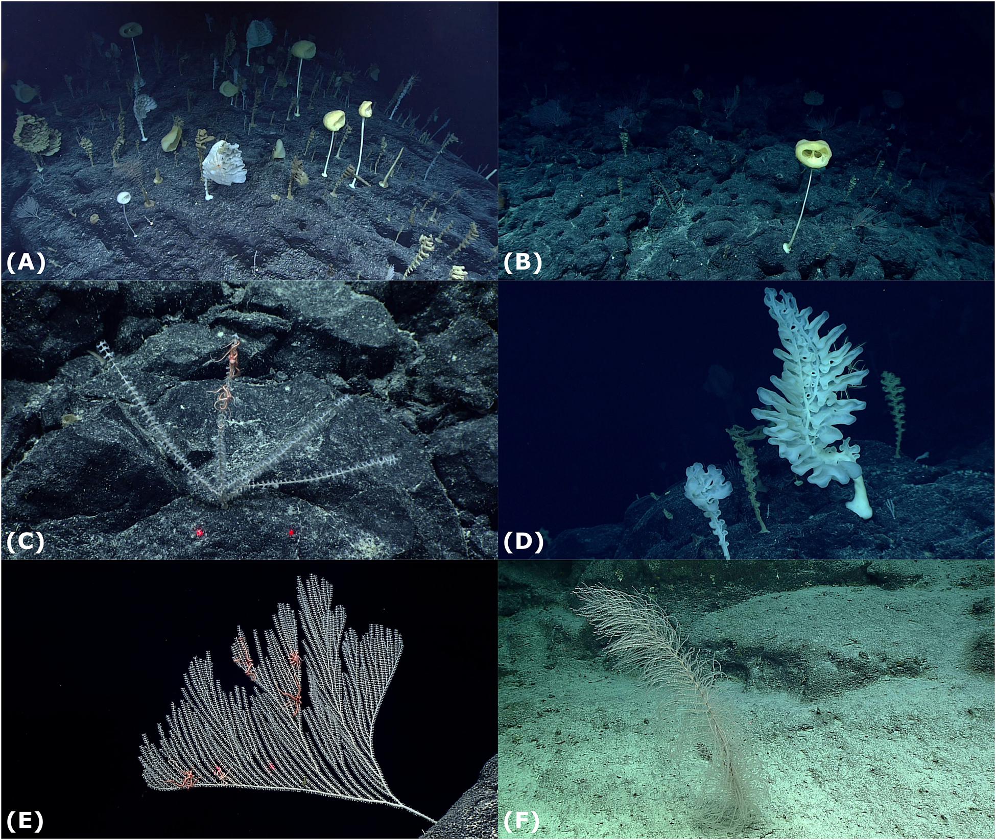
Figure 1. Different taxa identified within this study. Red laser dots are 10 cm apart. (A) A photograph of the Ridge Crest Area, (B) Advhena magnifica, (C) Narella macrocalyx, (D) Aspidoscopulia, (E) Narella bowersi, and (F) Rhodaniridogorgia.
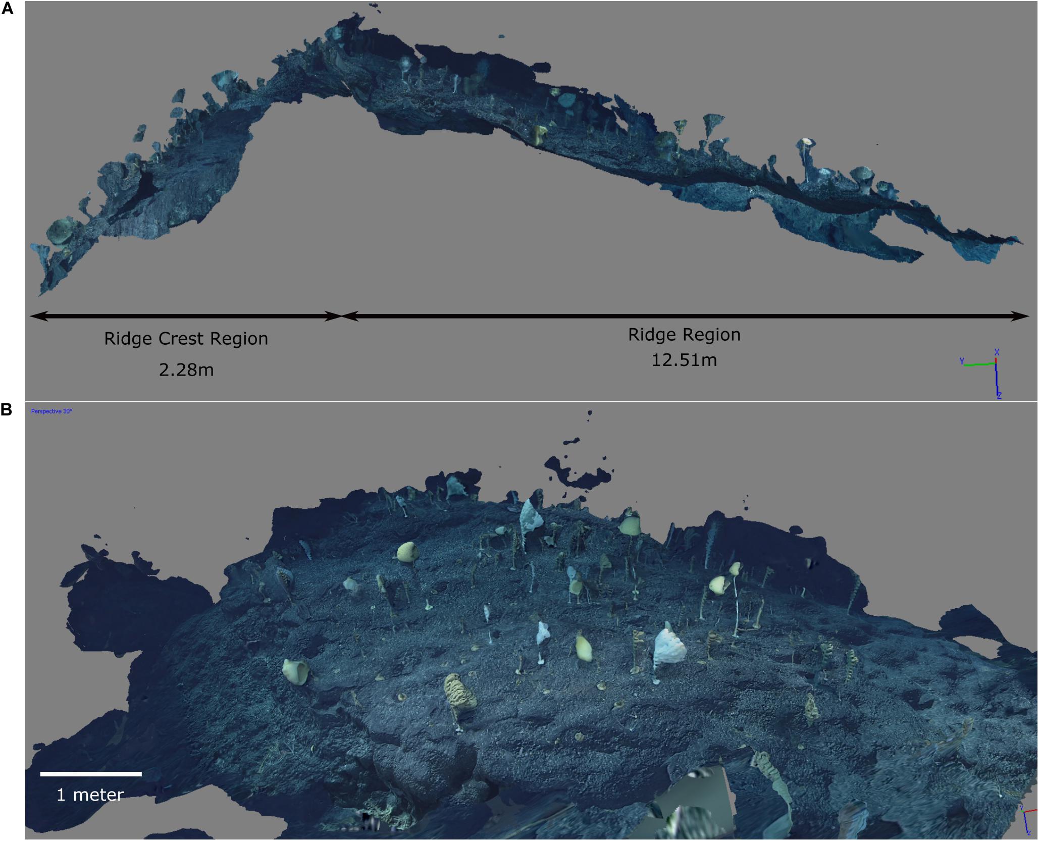
Figure 2. Screenshots of the 3D reconstruction. (A) Side view showing the two different areas with the Ridge Crest area on the left and Ridge area on the right. (B) A closer view of the Ridge Crest community. The dark blue areas above the community and rising to the left and right are artifacts of the photogrammetry where frames included a lot of the farground. The substrate beyond the edge of the ridge to the right and left has good resolution, and so the edge of the community is clearly resolved. Note the badly resolved section at the bottom of the screenshot, where there wasn’t sufficient video coverage to reconstruct the substrate (which was sparsely populated).
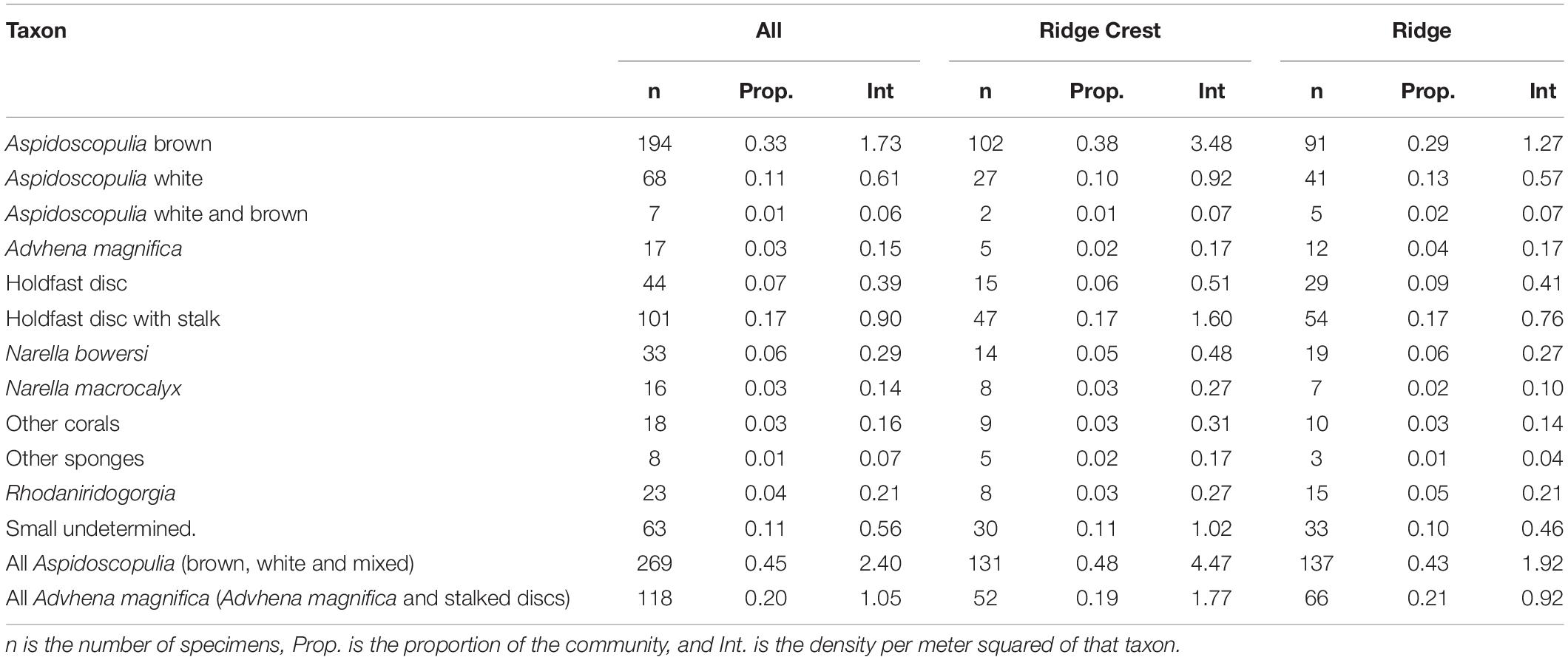
Table 1. Summary table.
With the advent of high-resolution ROV cameras and high-powered computers, it is now possible to reconstruct entire benthic communities using photogrammetry to centimeter or millimeter scale (Robert et al., 2017, 2020; Baker et al., 2019; Prado et al., 2019; Price et al., 2019), so providing greater accuracy and resolution than the meter scale of ROV location data alone (Kennedy et al., 2019). These 3D photogrammetric reconstructions avoid the problems of controlling for altitude that often accompany 2D photo-montages because the triangulation of points using photographs from multiple angles limits the possible errors—if there is not enough photographs to accurately reconstruct the area, then the 3D model will not be generated (see Robert et al., 2017 for further details). However, errors can be introduced due to specimen movement, which occurred for this dataset, so size analyses were not performed.
The video recorded from the ROV was 720p five mega-bit per second resolution (Malik et al., 2018). The 3D reconstruction of the FW community was created using photogrammetry in Agisoft Metashape 1.5.4 (formerly Agisoft Photoscan) following a similar procedure to Robert et al. (2017), with the 2D projections of the reconstruction performed in Geomagic Wrap 2015.
1. The start of the FW community was taken to be from the ROV track starting at 14°28′24.156″ N, 170°51′18.231″ W until 14°28′24.198″ N, 170°51′17.553″ W.
2. The edges of the community were taken to be the edges of the ridge. There were organisms outside this region, but the reconstruction did not have sufficient tie point matches to reconstruct the region accurately.
3. This segment of video was sampled at a capture rate of 1 frame/second using ffmpeg—an open source video encoder/decoder.
4. Out of focus and shaky frames were removed, as were frames that were close up of individual specimens and/or had other objects obstructing the view in the frame.
5. The files were then imported into Agisoft Metashape.
6. Chunks of 100 frames were auto-aligned to form a sparse point cloud.
7. These chunks were then aligned into the complete community which was formed from 583 out of a total 600 input frames and 131,322 tie points.
8. A dense cloud (6 million points) and mesh (4.398 million faces) was created from the combined sparse point cloud.
9. The frames were matched to the ROV GPS tracks by using the epoch timestamp in the GPS log and matching it (using a “join query” in Access) to the image frames, which had been renamed to match. Distances were checked using photographs where 2 red laser dots (10 cm apart) to correctly scale the reconstruction.
10. Individual organisms were marked up and identified on the frames within the 3D reconstruction. Note that the resolution of the videos was less than that of the high-resolution photographs taken which hinders resolution for smaller specimens and also meant that very small (∼<2 cm) specimens may not have been marked.
11. Specimen positions were checked from multiple viewpoints.
Screen shots of the 3D reconstruction show both the strengths and weakness of the reconstruction (Figure 2). Generally the substrate and the attachment to the substrate are well resolved. The video footage focused on the ridge so that areas outside the ridge were not well resolved (and thus not included in the analyses). However, the edge of the ridge is clearly visible, and shows a notable decrease in density. The dark blue areas were the deep far-ground which was not sufficiently well resolved to be accurately reconstructed. The organisms’ tops often appeared disconnected from their base, probably due to movement, but it was straightforward to infer which holdfast they belonged to.
In order to get the 2D map for our analyses, the 3D reconstruction was exported into Geomagic Wrap, and a best-fit plane was fit to the Ridge and Ridge Crest areas, respectively. The 2D maps for each area were created by rotating the specimen positions to the best-fit planes for each section separately, which were then exported then rejoined as a single 2D projection (see SI for data).
Four different types of spatial analyses were performed on the data: (1) Random labeling analyses were used to investigate the mortality dynamics within the community. (2) Univariate SPPA were used to investigate the population ecology of each taxon. (3) BNI was used to identify primary dependencies between taxa. (4) Bivariate SPPA was used to determine the most likely underlying processes to the primary dependencies found using BNI.
The simplest scenario within SPPA analyses is that all the points (here different organisms) are randomly distributed within the study area. This random distribution is known as complete spatial randomness (CSR), and can be modeled as an homogeneous Poisson model (Illian et al., 2008). Where CSR is found to best describe the spatial distributions observed, there are no biotic and abiotic processes which significantly effect that population at the spatial scales considered. If the spatial distributions are non-CSR, then they can be aggregated, whereby the organisms are closer together than CSR; or segregated, where the organisms are more spaced out than CSR. Non-CSR distributions could also have aggregation and segregation operating at different spatial scales, which is reflecting different processes operating at different scales. Univariate or single population aggregations can be caused by habitat associations, where the taxon has an environmental preference, such as altitudes for alpine tree species (Wang et al., 2012), and these habitat associations are best modeled by heterogeneous Poisson models (Wiegand et al., 2007b; Wiegand and Moloney, 2013). Habitat associations can also cause univariate and bivariate segregation when the habitat which the taxon/taxa occupy is itself segregated (Mitchell and Kenchington, 2018). Univariate aggregations can also be caused by dispersal processes, whereby offspring surround their parent (Mitchell et al., 2015), and these are best modeled by Thomas cluster models for a single reproductive event, or double Thomas cluster models for two reproductive events (Wiegand et al., 2007b; Illian et al., 2008). Habitat associations can also result in bivariate (between two taxon) aggregations, which can be best modeled by heterogeneous Poisson models or shared source models (also called shared parent models) where the two sets of taxon aggregate around the same set of mutually exclusive points, i.e., the focus of the taxon clusters are points that are not biological taxa, but some other “environmental” factor (Wiegand et al., 2007b; Wiegand and Moloney, 2013). Bivariate aggregations can also be caused by facilitation whereby one taxon increases another’s chance for survival, and is modeled as a linked Thomas cluster model, with aggregations of the facilitated taxon centered on the facilitating taxon (Dickie et al., 2005; Getzin et al., 2006; Dale and Fortin, 2014). Alongside habitat associations, univariate and bivariate segregation also occurs through competition between organisms for resources (Wiegand et al., 2007a; Illian et al., 2008) where it can be modeled by hard-core (where there is no overlap of organisms within a given radius) and soft-core (where organism density is reduced) processes. While untangling processes from these spatial pattern is imprecise (Law et al., 2009; McIntire and Fajardo, 2009), the use of complementary types of SPPA with multiple model fitting and assessment means that the most likely underlying process can be inferred (Levin, 1992; Wiegand and Moloney, 2004, 2013; Illian et al., 2008; Waagepetersen, 2009).
Density-dependent mortality processes are best investigated using a subset of SPPA called Random Labeling Analyses (RLA) (Raventós et al., 2010). While density-dependent mortality processes can be detected through distance measures as described above, RLA is preferable because no assumptions need to be made about the processes underlying the initial spatial distributions, enabling the uncovering of subtle processes that may otherwise be obscured. Instead, the spatial distributions of the dead among the living are investigated in order to investigate whether the dead specimens are aggregated, indicating density-dependent mortality.
To investigate mortality processes, we investigated how a state of an organism (dead or alive in this study) changes within organism locations, using RLAs (Pélissier and Goreaud, 2001; Raventós et al., 2010). We followed methods similar to Mitchell et al. (2018). RLAs are a type of SPPA whereby random models are simulated whilst the positions of the specimens remain the same and a given property, such dead or alive, is repeatedly permutated: the points remain in the same place, but the state allocated to them (representing either dead or alive) is changed. As such, RLAs do not directly measure the aggregation or segregation between two populations, and so do not test the processes that resulted in sponge location, but instead measure the differences in spatial distributions of live/dead state between two populations.
Spatial distributions are commonly described using PCFs which describe how the density of points (i.e., sponge specimens) changes as a function of distance from the average specimen (e.g., Illian et al., 2008). RLAs assess the differences between two characters (dead/alive) of the populations by calculating variations between PCFs by considering the Difference and Quotient tests (Wiegand and Moloney, 2013). The Difference test is the calculation of the distribution of PCF 11 − PCF 22, where PCF 11 is the univariate PCF for group 1 and PCF 22 is the univariate PCF for group 2. If PCF 11 − PCF 22 = 0 then both groups are randomly distributed within the locations (i.e., both groups exhibit the same spatial behavior). If PCF 11 − PCF 22 > 0, then group 1 is more aggregated than group 2; if PCF 11 − PCF 22 < 0, then group 2 is more aggregated than group 1. To further investigate the differences between the dead and alive populations, the PCF 21 − PCF 22 and PCF 12 − PCF 11 are calculated. These differences test the relative aggregation (or segregation) of the dead and alive spatial distributions compared to the relative spatial distribution of the dead to alive (and vice versa). If PCF 12 − PCF 11 < 0 then group 1 (alive) are positively correlated with other alive points, and if PCF 21 − PCF 22 < 0 then group 2 (dead) are positively correlated with other dead specimens. The difference PCF 12 − PCF 21 was used to test for edge effects within the study area. If there are excursions outside the Monte Carlo simulations (as is common at larger spatial scales), then edge effects have a significant impact on the analyses, and the scales over which the analyses are done should be reduced.
The Quotient test calculates the bivariate PCF between groups relative to the pattern of both groups taken together (the joined pattern), where PCF12 is the bivariate distribution of group 2 relative to group 1 and PCF 21 is the bivariate distribution of group 1 relative to group 2. For joint patterns, PCF 1,1+2 is the bivariate distribution of group 1 relative to both groups together, and PCF 2,2+1 is the bivariate distribution of group 2 relative to the joint pattern. Thus, the Quotient test is the calculation of the distribution: PCF 1,1+2 - PCF 21/PCF 2,2+1 where PCF 12/PCF 1,1+2 - PCF 21/PCF 2,2+1 > 0 indicates that group 2 is mainly located in areas with high density of the joint pattern, and group 1 is in low density areas (i.e., group 2 has more neighbors than group 1). If this quotient is significantly non-zero, then the process underlying the characters is density-dependent; for example, dead specimens occur more commonly in high-density areas, indicating density-dependent mortality.
We test three null hypotheses of mortality spread using RLA of dead/alive state with the organism positions:
(1) H0Comm: The spatial distribution of dead specimens are randomly distributed within the living community of corals and sponges.
(2) H0Asp: The spatial distribution of dead specimens of Aspidoscopulia are randomly distributed within the living population of Aspidoscopulia.
(3) H0Bol: The spatial distribution of dead specimens dead specimens of within Advhena magnifica population are randomly distributed within the living population of Advhena magnifica.
Establishing whether the null hypotheses of the Difference and Quotient Tests should be rejected or not is complicated, because there is a lack of independence of the spatial points (organism positions) and a variety of different point pattern distributions (Illian et al., 2008). Two different methods are commonly used to establish acceptance or rejection of the null hypotheses for ecological data (e.g., Wiegand and Moloney, 2013 and references therein): (1) Monte Carlo simulations (Illian et al., 2008), and (2) Diggle’s goodness-of-fit test pd, which represents the total squared deviation between the observed pattern and the simulated pattern across the studied distances (Diggle, 2002; Diggle et al., 2005). The two comparisons are used together because: (1) the Monte Carlo simulation envelopes do not necessarily correspond to confidence intervals, and they run the risk of Type I errors if the observed PCF falls near the edge of the simulation envelope (Illian et al., 2008); (2) the pd does not strictly test whether a model should be accepted or rejected, but rather whether the test calculation for the observed data are within the range of the stochastic realization of the null hypothesis (Diggle, 2002); and (3) the pd depends on the range over which it is calculated, meaning that the model may not fit at very small distances due to the physical occupation of that space by the organisms themselves, but may fit well at larger distances (Diggle, 2002; Illian et al., 2008). Thus visual inspection of the PCFs with Monte Carlo simulation envelopes, coupled with pd, ensures that these errors are minimized. The underlying mathematics is described in detail by Wiegand and Moloney (2004, 2013) and Wiegand et al. (2006).
The following RLAs were conducted using Programita software across three different areas: All mapped area, the Ridge and the Ridge Crest (Wiegand and Moloney, 2004, 2013; Wiegand et al., 2006; Raventós et al., 2010):
(1) To test H0Comm all living specimens of both coral and sponge taxon were contained in the alive group and, and all brown specimens (including the dead Aspidoscopulia, holdfast discs with long stalks and holdfast discs) were grouped as dead. The univariate PCFs of the dead and the alive populations were calculated by creating a distribution map of each dead/alive state according to a 10 cm × 10 cm grid of surface within which the specimen density was calculated. The Difference tests were then performed between the two groups.
(2) To test H0Asp the white specimens of Aspidoscopulia were assumed to be alive, brown specimens dead and those with white and brown patches were excluded from the analyses (7 specimens in total so not sufficient to run separate analyses). Difference and Quotient tests were performed between the dead and alive groups. If the dead and alive specimens did not have significantly different spatial distributions when compared using the Difference test, they are most likely to be subjected to the same biotic and abiotic processes and so are likely to come from the same single population. If the Difference test finds no significant difference between the dead and alive populations, then the Quotient test was to determine whether the dead specimens are randomly distributed within this population.
(3) To test H0Bol the holdfast brown discs with long stalks were assumed to be the dead Advhena magnifica, and the yellow/white specimens were assumed to be alive. Testing proceeded as for H0Asp.
Each hypothesis was tested by running 999 Monte Carlo simulations for each group in order to generate simulation envelopes around the random PCF value (i.e., PCF 11− PCF 22 = 0). pd values were calculated using Diggle’s goodness-of-fit test (Diggle et al., 2003). A total of 999 simulations were run (instead of 1,000, for example) because the pd value is calculated using the model simulation data (not the theoretical model), and so by using 999 the pd simulations could be measured in 0.001 increments. If the observed PCF 11 − PCF 22 fell outside the RLA simulation envelopes and had pd < 0.1, then the distributions were found to be significantly different.
Initial data exploration and data visualization were performed in R (R Core Team, 2017) using the package spatstat (Berman, 1986; Baddeley and Turner, 2005; Baddeley et al., 2011). The software Programita (Wiegand et al., 1999, 2006; Wiegand and Moloney, 2004, 2013; Loosmore and Ford, 2006) was used to calculate the PCF and to perform aggregation model fitting (described in detail in Berman, 1986; Wiegand and Moloney, 2004, 2013).
The following analyses were performed on each abundant taxon (Aspidoscopulia, Advhena magnifica, Rhodaniridogorgia, Narella macrocalyx, and Narella bowersi) across the entire mapped area (All), the shallower section of the ridge (Ridge) and the steeper area of the ridge (Ridge Crest).
To test whether a taxon PCF exhibited CSR, 999 Monte Carlo simulations were run on a homogeneous background and the simulation envelopes chosen to be the 49th highest and lowest values (Wiegand and Moloney, 2013; Mitchell et al., 2018). The models were simulated around CSR, that is PCF = 1. The fit of the observed data to CSR was tested using Diggle’s goodness-of-fit test (Diggle et al., 2005) pd (where pd = 1 corresponds to CSR, and pd = 0 corresponds to non-CSR) with PCF deviations outside the simulation envelope combined with a pd < < 1 interpreted to indicate significantly non-CSR distributions.
If a taxon was not randomly distributed on a homogeneous background, and was aggregated, the random model on a heterogeneous background (HP model) was tested by creating a heterogeneous background from the density map of the taxon under consideration, being defined by a circle of radius R over which the density is averaged throughout the sample area. Density maps were formed using estimators in 0.10 m increments over the range of 0.1 m < R < 1 m, and the R corresponding to the best-fit model was used. The radius was increased to account for differing granularity of heterogeneity—the R = 0.1 m will model granular heterogeneities whereas the R = 1 m will be relatively smooth. If excursions outside the simulation envelopes for both homogeneous and heterogeneous Poisson models remained, then Thomas cluster models were fitted to the data as follows:
(1) The PCF and L functions (Levin, 1992) of the observed data were found. Both measures were calculated to ensure that the best-fit model is not optimized toward only one distance measure, and thus encapsulates all spatial characteristics.
(2) Best-fit Thomas cluster processes (Besag, 1974) (TC) were fitted to the two functions where PCF > 1. The best-fit lines were not fitted to fluctuations around the random line of PCF = 1 in order to aid good fit about the actual aggregations, and to limit fitting of the model about random fluctuations. Programita used the minimal contrast method (Diggle, 2002; Diggle et al., 2005; Wiegand et al., 2007b) to find the best-fit model.
(3) If the model did not describe the observed data well, the lines were refitted using just the PCF. If that fit was also poor, then only the L-function was used.
(4) 999 simulations of this model were generated to create the simulation envelope. The 49th highest and lowest simulation values were chosen in line with previous work to be the limits of the simulation envelopes (Wiegand and Moloney, 2013), and the fit was checked using the O-ring statistic (Wiegand and Moloney, 2004).
(5) pd was calculated over the model range.
(6) If there were no excursions outside the simulation envelope and the pd -value was high, then a univariate homogeneous Thomas cluster model was interpreted as the best model.
(7) The best-fit TC model was simulated on the best fit HP model following points 4–5 to simulate a Thomas cluster model on a heterogeneous background (ITC).
The Bayesian network inference (BNI) algorithm used in this study requires discrete data which ensures data noise is masked and only the relative densities of each taxon are important (Yu et al., 2002; Milns et al., 2010). Previous work has shown that ecological datasets using three different bins provide a good balance between maintaining the amount of information present in the dataset, statistical power, and greater noise masking (Yu, 2005; Milns et al., 2010; Mitchell et al., 2020a). The data were split into three intervals: zero counts, low counts and high counts. Zero was treated as a separate entity because the presence of one individual is very different to a zero presence, in contrast to zero gene expression, for example. Low counts consisted of counts below the median for the species group and high counts were counts over the median. Medians were used rather than means because for some groups the high counts were very high, and would result in a very small number of samples grouped in the highest interval (cf. Milns et al., 2010).
The BNI software used was Banjo v2.0.0, a publicly available Java-based algorithm (Smith et al., 2006). For details of the algorithm please see Smith et al. (2006) and Milns et al. (2010). Pre and post-processing was performed using custom scripts in Haskell (Jones, 2003)1 and in R (Mitchell, 2011; R Core Team, 2017). The discretized data was input into Banjo which then generated a random network based on the input variables. A “greedy search” was repeated 10 million times for each set of input data and the most probable network was then output. The maximum number of edges leading to a node was set to 3 to limit artefacts (Yu, 2005).
To convert the spatial positions of specimens into discretized data suitable for BNI analyses the following steps were taken (following (Milns et al., 2010):
(1) Node definition. The nodes were defined by taxa groups (Figure 1).
(2) Quadrat selection. Abundance data were calculated in terms of specimen density within quadrats (2 m × 2 m). This size of quadrat was chosen to ensure an even split between the three bins.
(3) Discretization. For each quadrat, taxon densities were split into three intervals: zero counts, low counts (under the median) and high counts (above the median) to capture the maximum amount of data information while masking noise.
(4) Contingency test filtering. To exclude false positive dependencies between taxa we used contingency filtering (χ2-tests, p > 0.25).
The discretized data for the BNI analyses are given in Table 2. To minimize bias from outliers, we bootstrapped at 95% level (Magurran, 2013) by randomly selecting 95% of the total number of grids cells for each subsample and then finding the subsample network using Banjo. For each edge calculated, the probability of occurrence was calculated as the proportion of the bootstrapped samples in which the edge appeared. The resultant distributions analyzed to find the number of Gaussian sub-distributions using normal mixture models (Fraley et al., 2012). This probability distribution was bimodal for each dataset, which suggests that there were two distributions of edges, those with low probability of occurrence, and those highly probable edges. The final network for each area was taken to be those edges which were highly probable. The threshold for being labeled “highly probable” was 55% for this dataset. The magnitude of the occurrence rate is indicated in the network by the width of the line depicting the edge.
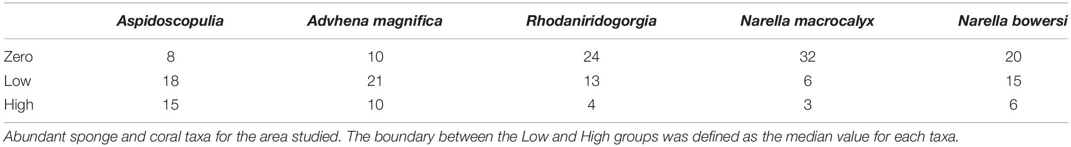
Table 2. Discretized data for BNI.
The direction of the edge between nodes in the network indicates which node (taxon) has a dependency on the other node (taxon); this direction is indicated in the network by an arrowhead. For each edge, the directionality was taken to be the direction which occurred in the majority of bootstrapped networks. Where there was no majority (directional edges have a probability between 0.35 and 0.65) an edge was said to have bi-directionality, or mutual dependency was indicated; these are shown without arrows.
The influence score (IS) can be used to gauge the type and strength of the interaction between two nodes. Positive dependencies have an IS > 0: that is, a high density of taxon 1 corresponds to a high density of taxon 2, and so the dependency arrow would point from taxon 2 to taxon 1. Negative dependencies have an IS < 0: a high density of taxon 1 corresponds to a low density of taxon 2. Where the dependency is non-monotonic the IS = 0 so that nature of the dependency changes with taxon abundance. The mean IS for each edge was calculated for each site.
For every dependency found between taxa by BNI, bivariate SPPA were used to infer the most likely underlying processes (cf. Mitchell and Butterfield, 2018).
Bivariate PCFs were calculated from the population density using a grid of 10 cm × 10 cm. To minimize noise, smoothing was applied to the PCF dependent on specimen abundance. The amount of smoothing required depends on the number of points in each taxon’s population, with smaller sample sizes requiring more smoothing to ensure that outliers do not overly change the distribution (Illian et al., 2008; Wiegand and Moloney, 2013): A five cell smoothing over this grid was applied to Aspidoscopulia—N. bowersi, six cells to Advhena magnifica—N. bowersi, and seven cells to N. macrocalyx—N. bowersi, across the entire mapped area (All), the shallow section of ridge (Ridge) and the steeper area of the ridge (Ridge Crest) (Figure 2).
For each taxon pair which displayed aggregation (bivariate PCF > 1), CSR, HP, Linked clusters (LC) and shared parent (SP) models were fitted to the data. For segregated bivariate distributions (bivariate PCF < 1), CSR, HP, hard and soft core models (HC), and hard/soft core on heterogeneous background (HCHP) models were fitted as follows. The magnitude of the PCF reflects the intensity of underlying biotic and abiotic processes: two taxon populations with a PCF = 4, for example, are four times more aggregated than if they exhibited CSR; thus, the relative magnitudes of the PCFs can be used to compare relative strengths of interactions and associations.
If a taxon was aggregated, the random model on a heterogeneous background (HP model) was tested. Creation of the heterogeneous background was as for the univariate distribution, but instead of a single taxon, the density map of the joint distribution of the two taxon was used.
For each taxon pair, two best-fit Linked cluster models (LC) were found. First, Taxon 1 was kept constant and Taxon 2 was modeled as a Thomas Cluster aggregation around Taxon 1 (following the same procedure as fitting univariate TC models). Then Taxon 2 was kept constant and Taxon 1 was modeled as an aggregation. The shared parents models (SP) modeled both taxa distributions as Thomas Cluster models around randomly distributed shared points, with the respective Thomas Cluster models fitted as per the univariate models.
Segregated distributions were modeled on both homogeneous background and on heterogeneous background. Three different models were determined: Segregation around Taxon 1, around Taxon 2 and around both Taxon 1 and Taxon 2. For each of these the radius was increased from 0.10 m to 1.00 m in 0.10 m increments. The severity of the segregation was modeled in two ways: hard and soft-core. For hard-core models (corresponds to HCp = 0.01), no points are modeled inside the segregation radius while for a soft-core model the density of points within the segregation radius was reduced by a given probability. Where HCp = 1 the probability of placing points is a linear relationship from the point to the radius edge, and is defined by the formula (Wiegand and Moloney, 2013; Getzin et al., 2014): phc(r) = d 1/p.
The mapped community consisted of 592 specimens over 100.7 m2 of substrate. The community was dominated (69.7%) by two genera of Hexactinellids: Farreidae Aspidoscopulia sp. and Euplectellidae Advhena magnifica with octocorals Narella bowersi, Narella macrocalyx, and Rhodaniridogorgia also present in large proportions (Table 1). There was significant increase in organism density between the Ridge and Ridge Crest (4.47 vs. 9.28 specimens/m2) which were split into two different sub-areas of 71.41 m2 for the Ridge area and 29.31 m2 for the Ridge Crest area for further analyses (Table 1 and Figure 3). Community composition remained similar across both areas, with a < 0.5% mean change in taxa proportions between the two areas (Table 1).
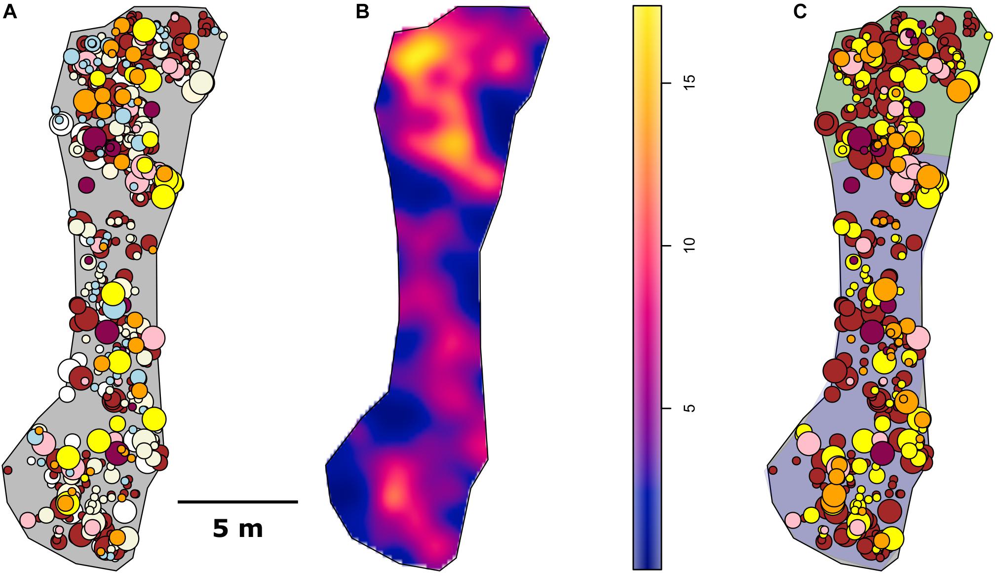
Figure 3. Spatial maps. (A) All specimens identified, (B) Density map of the 2D project in square meters, and (C) the analyzed data. Shaded area of (C) in purple is the Ridge area and green is the Ridge Crest area.
Analyses to detect edge effects (Table 3: PCF 12 − PCF 21) found that for the Aspidoscopulia population, edge effects occurred over 4.3 m. Therefore, the spatial scale was limited to 0–4.0 m for all plots to enable consistent comparisons.
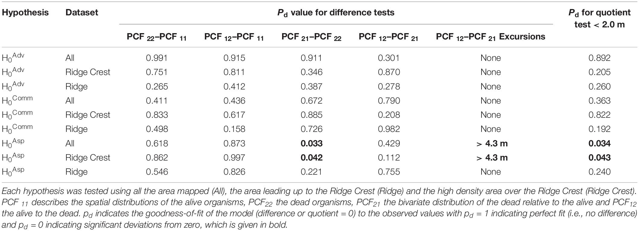
Table 3. Random labeling analyses.
Within the whole community there was no evidence of significant deviations from zero for any of the RLAs (Figure 3A), that is the dead specimens were randomly distributed within the living communities (all pd > > 0.1), so we fail to reject H0Comm. The Advhena population and stalks also did not display significant deviations from zero (all pd > > 0.1; Figure 3C). Furthermore, the differences of the univariate distribution of Advhena with the univariate distribution of stalks had a very good model fit to zero (pd = 0.991), which provides confirmatory evidence that the stalks are likely to be the dead skeletons of Advhena.
The RLAs of the Aspidoscopulia population found no significant deviations from zero for the difference between the univariate alive and dead Aspidoscopulia populations (all PCF 22 − PCF 11 pd > > 0.1, Figure 3B) nor the bivariate difference (all PCF 12 − PCF 21 pd > 0.1). The difference between the univariate alive Aspidoscopulia and the bivariate distributions was also not significantly deviate from zero (all PCF 12 − PCF 11 pd > 0.1). There were significant deviations from zero for the Quotient tests (Figure 3B) for the population across the whole sample area (pd = 0.034), and in the high density Ridge Crest area (pd = 0.043), but notably not in the Ridge area (pd = 0.240). This pattern is further reflected in the Difference tests (PCF 21 − PCF 22) which found that the difference of bivariate distribution with the dead univariate did deviate significantly from zero (Table 1) for the whole area (pd = 0.033), and in the high density Ridge Crest area (pd = 0.042) but not the Ridge area (pd = 0.221). The significant deviations in the whole area are likely to reflect the signal from the Ridge Crest sub-section. Within the Ridge Crest section dead specimens of Aspidoscopulia were more likely to be found near each other than near living specimens, and these dead specimens occurred in the higher density areas of the joint distribution of alive and dead specimens. In contrast, the dead specimens did not show significant aggregations to each other or to high density areas within the Ridge sub-section of the mapped area.
Rhodaniridogorgia was the only taxon to have a good model-fit to the CSR model (pd = 0.704), although the HP model (pd = 0.825) was a better fit (Table 4). The Monte Carlo simulations showed no deviations outside the envelope (Figure 5E), so the Rhodaniridogorgia spatial distribution should be described as CSR. Of the four of the abundant taxa that exhibited non-CSR best-fit models, Advhena magnifica had the same best-fit model (HP) for both the Ridge (pd = 0.817) and Ridge Crest sections of the mapped area (pd = 0.562), with significant segregations occurring over 1.3 m for the Ridge section and over 3 m for the Ridge Crest regions (Figure 5C and Table 4). The Aspidoscopulia (Figure 5D and Table 4) had a best-fit model of Thomas cluster models for both Ridge (pd = 0.727) and Ridge Crest sections of the mapped area (pd = 0.547) with a segregation in the Ridge area over 1.2 m. In contrast, the N. macrocalyx displayed different spatial distributions in the Ridge and Ridge crest area (Figure 5A and Table 4). The Ridge Crest area was best-modeled by a Thomas Cluster for the aggregations < 1.1m (pd = 0.375), and showed a strong segregation above 1.1 m, whereas the Ridge area was segregated under 0.7 m, and the aggregation above 0.7 m was best-modeled by a heterogeneous Poisson model (pd = 0.848). The N. bowersi also exhibited different spatial distributions between areas (Figure 5B and Table 4), with the Ridge Crest area showing strong aggregation best-modeled by a heterogeneous Poisson model > 1.3 m (pd = 0.761) whereas the Ridge area showed strong segregation < 1.3 m (pd = 0.729).
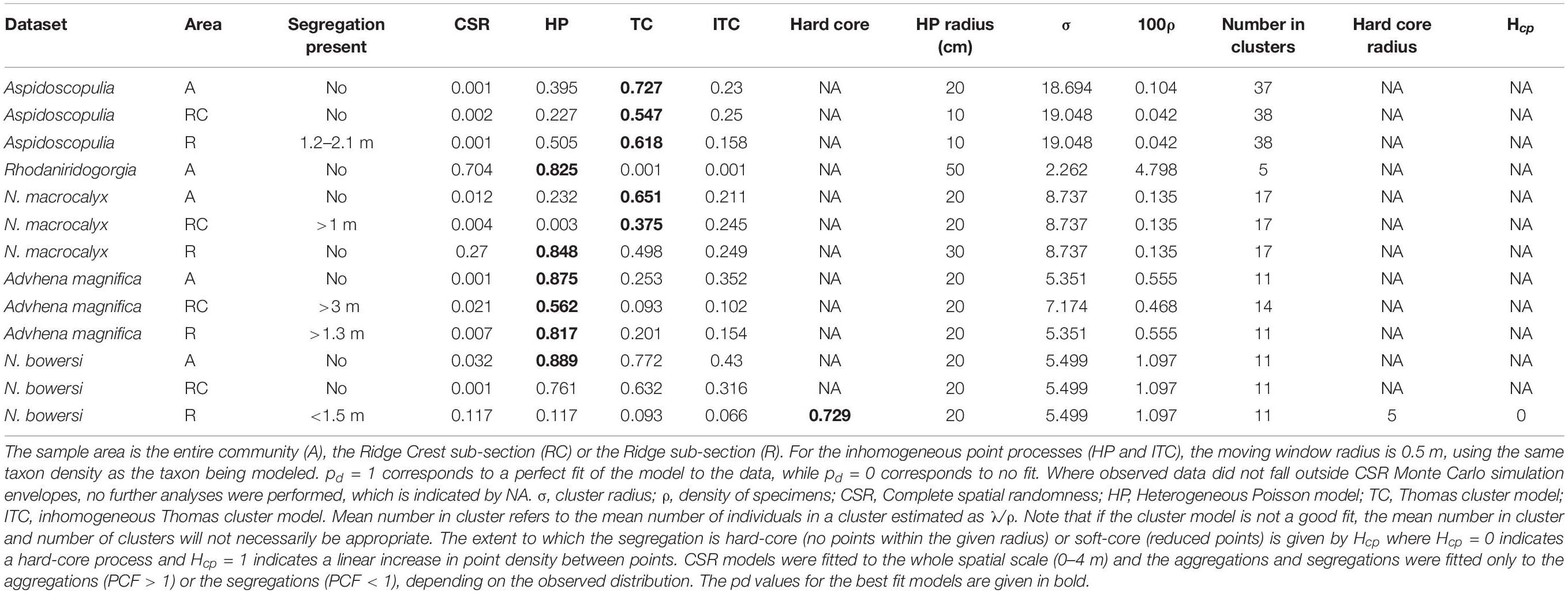
Table 4. Summary table of univariate PCF analyses.
The Bayesian network inference found three significant dependencies between four of the five abundant taxa (Figure 6), with Rhodaniridogorgia not connected to the network. Rhodaniridogorgia also showed a good CSR model fit for the univariate distributions (Figure 5E and Table 4). All three of the dependencies found were positive with a mean interaction strength of IS = 0.3109. Narella bowersi had a dependency upon Aspidoscopulia (IS = 0.3454), while both Advhena and N. macrocalyx had dependencies upon N. bowersi (IS = 0.3139 and IS = 0.2735), reflecting similar levels of dependency for all connected taxa.
The bivariate distribution for N. bowersi—Aspidoscopulia was best-modeled by a heterogeneous Poisson process of their joint densities across both Ridge (pd = 0.896) and Ridge Crest sections of the mapped area (pd = 0.817) which were aggregated at distances over 2 m (Figure 7A and Table 5). There was significant segregation for the Ridge Crest area over 2.8 m but no significant segregation in the Ridge area. For the N. bowersi—Advhena distribution, the best-fit model was a linked cluster model (Figure 7B and Table 5), with the Advhena clustering around the N. bowersi for both the Ridge (pd = 0.823) and Ridge Crest areas (pd = 0.631). The N. bowersi—N. macrocalyx displayed aggregation best-modeled as heterogeneous Poisson < 1.0 m for the Ridge area (pd = 0.912) and segregation < 1.2 m for the Ridge Crest area (pd = 0.841).
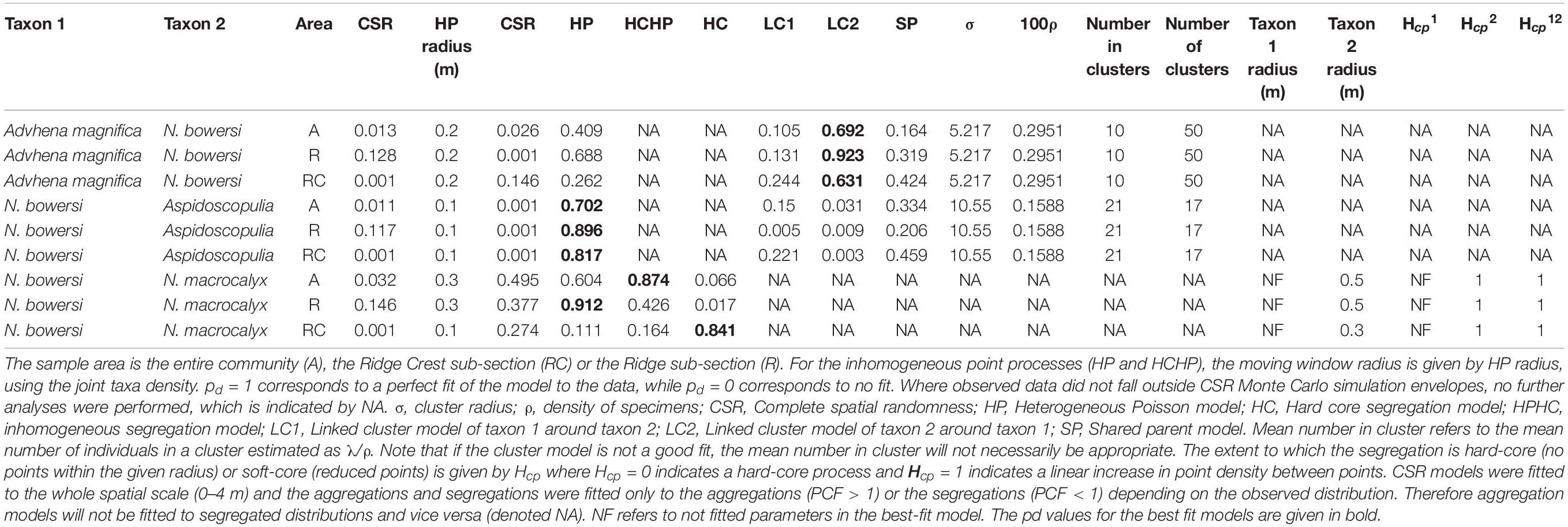
Table 5. Summary table of bivariate PCF analyses.
This study reconstructed the 592 specimens over 100.7 m2 of the benthic community of “The Forest of the Weird” from still frames taken from a single stream of video footage using photogrammetry methods (Figure 3). There were limitations to the data we could extract from the reconstruction. Our methods accurately reconstructed the sea floor, but the reconstruction of some organisms was more variable due to shadowing or movement. Shadowing occurred where the video footage had not captured all the way around an individual, and so the software needed to approximate the missing data. Movement caused a blurring of specimens and/or stalks to be absent. These issues meant that while the position data was likely to be accurate, size data was less so, and so size-based SPPA was not performed on this data. The lack of size data precludes more detailed analyses of community development. The reconstruction was done using the video data which had a lower resolution than the still photographic data and so we were able to use the photographs to compare to the stills extracted from the video. The two consequences of using the lower resolution video were: (1) that small white specimens (<1 cm) may not have been distinguished from the substrate and (2) it was hard to consistently identify different taxonomic groups for smaller specimens. We focused on the most abundant taxa, sponges and those corals which could easily be distinguished by distinct morphologies, which limits more detailed analyses of community composition and diversity. Nonetheless we were able to establish the mortality dynamics and spatial ecology of the five most abundant taxa.
This study has demonstrated how SPPA and BNI provide two new types of insights into the ecology of deep-sea benthic systems. First, SPPA can detect many different types of interactions and associations without any a priori knowledge nor expectations of the system. For example, SPPA was able to detect both the competition between N. bowersi—N. macrocalyx, the facilitation of the Advhena magnifica around the N. bowersi, and the habitat associations between N. bowersi—Aspidoscopulia (Figure 7 and Table 5). Secondly, SPPA enables the quantification on a continuous scale of interactions and associations from centimeter to meter scale, establishing at what scale the type of interactions may change, such as N. bowersi—Aspidoscopulia changing from a mutual habitat association to competition around 3 m (Figure 7B).
A high proportion (37.5%) of the specimens mapped were dead glass sponge skeletons (Table 1). The majority of dead specimens within the community were either the stalks of Advhena or dead Aspidoscopulia. Of the two possible causes of sponge death, age-related mortality or a pathogen, our results suggest that a species-specific pathogen is most likely. The univariate spatial distributions of the dead specimens is not statistically significantly different from the alive specimens (Table 3, PCF 22 − PCF 11) for either of the sponge species. Aspidoscopulia are best-modeled by a Thomas Cluster model (Table 4), which describes reproductive events (Seidler and Plotkin, 2006) so that if these sponges died due to age-related mortality, we would expect the dead specimens to have the spatial distributions corresponding to previous generations (cf. Mitchell et al., 2015). As such, the dead and alive specimens should have different univariate spatial distributions, and because they do not (Table 3), it is more likely their death is due to a pathogen. Advhena exhibited a non-dispersal spatial pattern so we can’t be sure that they were also killed by this pathogen over age-related mortality. However, the unusually high proportion of dead specimens and the presence of a mass-mortality pathogen for the Aspidoscopulia suggests that a pathogen cause is likely. While the remains of holdfast discs (12.9% of the dead specimens mapped) were not taxonomically identifiable, they resembled the Advhena and Aspidoscopulia holdfasts. The lack of density-dependent mortality (non-random RLA) for the Advhena magnifica and the Ridge area Aspidoscopulia suggests that the pathogen was likely to be water-borne, since transfer via mobile organisms or physical touching of specimens results in mortality clusters (Jolles et al., 2002).
The Advhena mortality was randomly distributed throughout both the Ridge and Ridge Crest areas of the communities (Table 3 and Figure 4). However, the mortality dynamics were different for the Aspidoscopulia, with the Ridge community showing random mortality, but the Ridge Crest community showing significant aggregations of the dead specimens relative to the living ones (Figure 4 and Table 3). Aspidoscopulia in the Ridge Crest area had a notably higher density than the Ridge area (4.47 vs. 1.92/m2) and a higher proportion of dead to living specimens (77 vs. 66%), suggesting that the presumed pathogen was spreading faster in these high density areas, but only for the Aspidoscopulia. If this difference was due just to density (i.e., not taxon specific) we would expect the Advhena to also have density-dependent mortality, as would the community as a whole, but instead it seems to be Aspidoscopulia specific, suggesting a lower resistance to the pathogen in these high density areas.
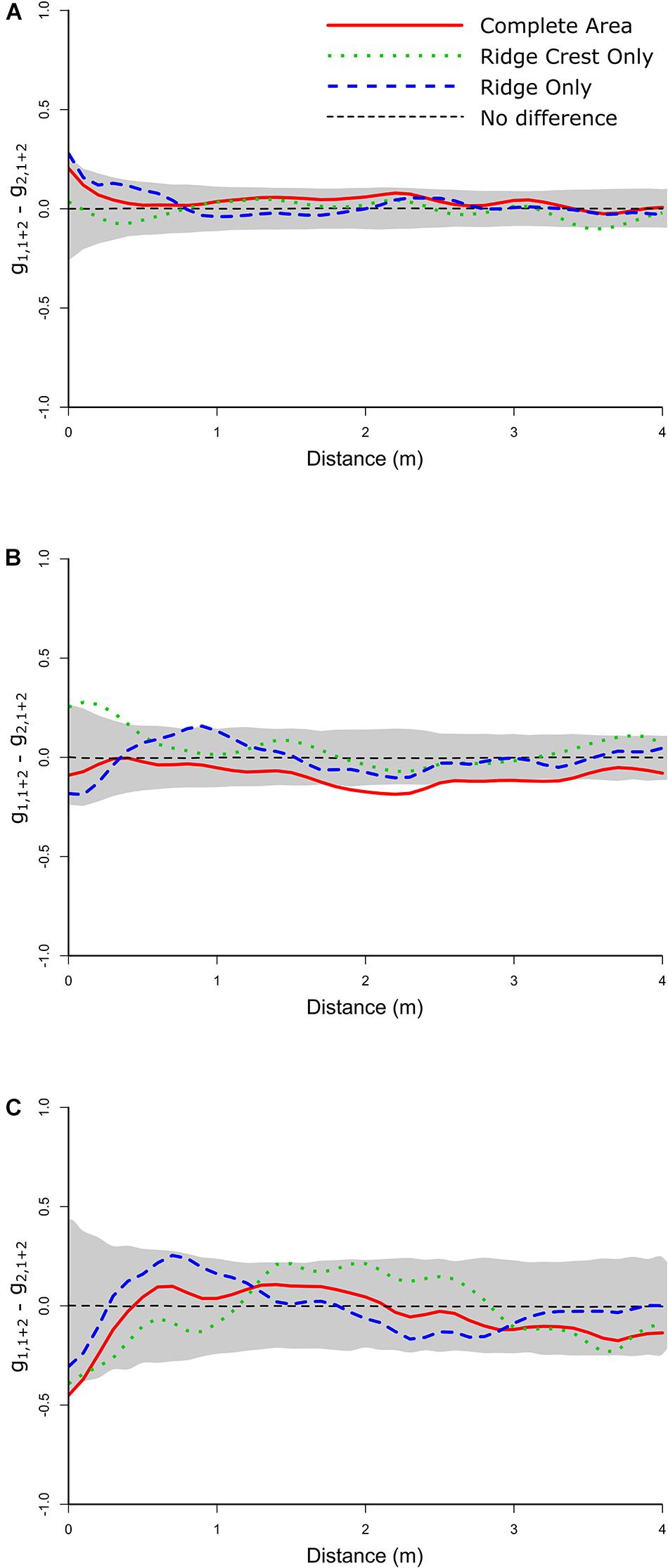
Figure 4. Random labeling analyses plots showing the Quotient test. (A) Whole community analyses of the dead population relative to the alive population (including all corals and sponges mapped) showing no significant deviations from zero. (B) The Aspidoscopulia analyses of dead vs. alive specimens. Note the whole community and the Ridge Crest sub-section both show excursions outside the simulation envelopes. (C) The Advhena magnifica analyses of dead vs. alive specimens showing no significant deviations from zero.
The Janzen-Cornell hypothesis is an explanation of how high diversity is maintained in tropical forests and coral reefs, whereby species-specific predators or pathogens are attracted to adults and/or high density areas resulting in high mortality surrounding the adults or in the high-density areas (Janzen, 1970; Connell, 1971). Within sponge communities, species-specific disease prevalence has been suggested as a mechanism to help maintain balance in abundance between species (Wulff, 2007). The species-specific mortality then enables different species to occupy these areas. Most studies testing this hypothesis are focused on shallow-water reefs, and have found no density-dependent mortality for giant barrel sponges (Deignan and Pawlik, 2015), Caribbean sponge Aplysina cauliformis (Easson et al., 2013) nor Caribbean corals (Muller and van Woesik, 2012), but density-dependent death due to corallivory has been detected in Indo-Pacific corals (Gibbs and Hay, 2015). In our study, we find that species-sensitive density-dependent mortality is likely once a density threshold was reached for Aspidoscopulia. The mortality within this community was likely to be a mass-mortality infection rather than a longer-term endemic pathogen because of the high proportion of dead skeletons coupled to relatively few dying specimens (those with brown patches (cf. Luter et al., 2017). In order for the Janzen-Cornell hypothesis to explain this high density community, we would expect episodic infections, so populations build up through time; thus any effects of this species-specific mortality would only become apparent if there were frequent mortality events. At the broad taxonomic levels used in this study, the two areas (Ridge and Ridge Crest) show significantly different densities, but similar community compositions (Table 1), suggesting that either this mortality event was rare, or if such events were frequent, then it did not lead to increased diversity (at least in terms of the coarse taxonomic identification used here). Further study of this site and other sites with similar community compositions may be able to elucidate whether such pathogens are likely to contribute to Janzen-Cornell effects.
Mass-mortality events and sponge diseases are on the increase (Webster, 2007) but have been primarily reported from shallow water sponge populations (Luter and Webster, 2017). The underlying causes are suggested to be anthropogenic changes, such as increasing temperature, which increase the susceptibility of benthic organisms such as corals and sponges to diseases through either a weakening of the organisms and/or an increase in pathogen virulence or abundance (Muller and van Woesik, 2012; Luter and Webster, 2017). The death of slow-growth sponges creates unoccupied patches which are often re-populated by faster-growing species (cf. Dayton, 1989; Dayton et al., 2013; Di Camillo and Cerrano, 2015). Sponges provide many ecosystem services, and while some services, such as providing habitat, can be replicated by other taxa (Buhl-Mortensen et al., 2010), sponges are crucial to oceanic mixing and benthic-pelagic coupling (Pile and Young, 2006; Bell, 2008; Coppari et al., 2016) which may be harder to replicate if they are replaced by organisms which do not pump water through their system. As such, there is potential for these deep-sea sponge diseases to impact the extent of benthic-pelagic coupling.
The FW community showed a clear increase in density and change of composition on the Ridge (seen in the 3D reconstruction at the edge of Figure 2, and noted on the ROV dive; Kelley et al., 2018). Furthermore, the sharper slope of the area after the Ridge Crest showed a large increase in density (Table 1) corresponding to faster water speed, and so probably to greater water-column resources (Malik et al., 2018).
The strength of SPPA lies with describing how the density of different taxa change over the fine scale (here 0–4 m), and then using model fitting to determine the most likely underlying processes. When spatial models such as heterogeneous Poisson models, heterogeneous Thomas cluster models or hard/soft-core models are the best-fit to observed spatial patterns, this suggests that abiotic or habitat heterogeneities are the strongest influence on the studied populations (Illian et al., 2008; Lin et al., 2011; Wiegand and Moloney, 2013; Mitchell et al., 2019). In contrast, random models or Thomas cluster models reflect biological patterns (Illian et al., 2008; Lin et al., 2011; Wiegand and Moloney, 2013; Mitchell et al., 2015), so that by fitting these different models to the observed data we were able to infer for each taxa whether biotic or abiotic effects had the biggest influence. At these fine-spatial scales we found that abiotic influence of habitat heterogeneities were the strongest driver for the majority of the populations studied. Abiotic heterogeneous Poisson models and hard-core models were the best fit for the observed spatial distributions for the populations of Advhena, N. bowersi, and Rhodaniridogorgia [although the small numbers of specimens, and lack of deviations outside the simulations envelope for Rhodaniridogorgia, means that this model was not significantly better than the random (biotic) model (Table 4 and Figure 5)]. For N. bowersi the interaction with the local habitat changed between the Ridge and Ridge Crest area, with the Ridge area showing significantly more segregation and thinning of organisms, reflecting a likely resource limitation due to lower water flow. The best-fit heterogeneous Poisson models for the N. macrocalyx, N. bowersi, and Advhena populations were over the same spatial scales of 20 cm, suggesting the same underlying habitat heterogeneity for all three taxa. While it is not analytically possible to determine what this heterogeneity is using our data, the topological variation of the basalt bedrock is of a similar scale, and so is a likely contender (Figures 1, 2).
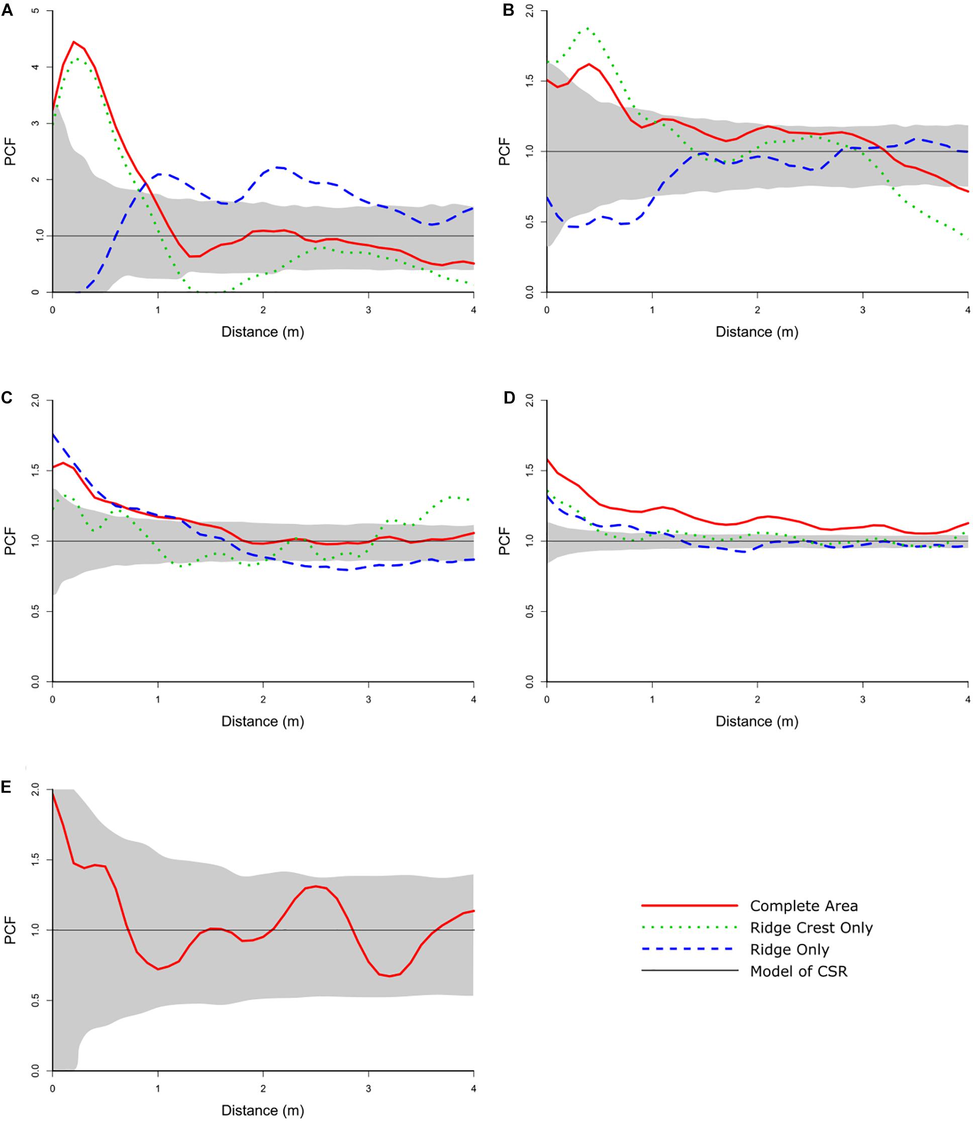
Figure 5. Univariate PCF for the abundant taxa. (A) Narella macrocalyx, (B) Narella bowersi, (C) Advhena magnifica, (D) Aspidoscopulia, (E) Rhodaniridogorgia. The gray area is the simulation envelope for 999 Monte Carlo simulations of complete spatial randomness. The x-axis is the inter-point distance between organisms in meters. On the y-axis PCF = 1 indicates complete spatial randomness (CSR), < 1 indicates segregation, and > 1 indicates aggregation.
In contrast Aspidoscopulia showed little sensitivity to these habitat heterogeneities, and instead the population spatial distributions reflected dispersal clusters. Narella macrocalyx was unusual in this community because the factors which most influenced its spatial distribution changed between the two community areas. In the Ridge area of the community N. macrocalyx was most strongly influenced by abiotic factors (habitat heterogeneity), but in the Ridge Crest area biotic factors (dispersal limitations) dominated. This change in influence is likely to reflect resource limitation in the lower-density Ridge area reducing the survival of juveniles, so that only the ones that settled on the optimal habitat remain. In the Ridge Crest region sufficient resources from increased water-flow result in higher survival rates, and so are a closer reflection of the original dispersal clusters.
The population ecology of the two sponges Aspidoscopulia and Advhena remained remarkably similar between the Ridge and Ridge Crest areas of the community, despite a doubling of population densities showing a lack of sensitivity to meter-scale variations in ridge topological and water-flow speed. In contrast, the octocorals N. macrocalyx and N. bowersi both showed significant differences in their spatial distributions, reflecting a higher sensitivity to these abiotic factors. The change for N. macrocalyx from an abiotic to biotic influence with increased density demonstrates the interplay between different driving forces and suggests that for at least some populations, different effects drive population under different conditions highlighting the need to record multiple different populations to understand the factors which underlie their dynamics.
Evidence for competition between marine sponges leading to elimination of a species are relatively rare, and most commonly involve outcompeting for a limited substrate, overflowing or chemical mediation (Wulff, 2007). This study has found subtle evidence of both intra and inter-specific competition. The large-scale segregation of the Aspidoscopulia, Advhena, N. bowersi, and N. macrocalyx suggests that a thinning of the populations is associated with increased competition for limited resources as organisms grow—they do not compete as juveniles but as they increase in size, they need more resources, and when they outcompete their neighbors, this leads to a reduction or thinning of the density (Getzin et al., 2006; Lingua et al., 2008). N. bowersi also has small-scale segregation reduction of 50%, which is likely to reflect intra-specific competition of juveniles, rather than mature organisms (Getzin et al., 2006, 2014). If the system is stressed, for example through reduction in the nutrients for which the organisms compete, then the strengths of competition are likely to increase, potentially leading to elimination of the weaker taxa.
Community composition for deep-sea sponge and coral communities is strongly driven by abiotic factors over broad scales (∼1–100 km) (Murillo et al., 2020). High density and very high density Pacific benthic communities show strong associations with temperature and geography (Hourigan et al., 2020). Despite a dramatic difference in community density between the two sections of the community at FW there remains a remarkable lack of differentiation of community composition (Table 1), showing a certain robustness in response to differences in ridge topography. This composition similarity, which is admittedly at a very coarse taxonomic scale, is unlikely to persist over long time scales due to density-dependent death of Aspidoscopulia in the Ridge Crest area (in contrast to the Ridge area and the random mortality patterns of Advhena). This density-dependent death has resulted in a different distribution of living Aspidoscopulia, and has provided a biogenic structure for sponge Poliopogon sp. which has grown on the top of the dead specimens (cf. Beazley et al., 2015). The BNI analyses showed that four out of the five abundant taxa were interconnected, with N. bowersi the most connected taxon (Figure 6). This connectedness means that if one taxon changes abundances, the other abundant taxon will also be affected—the density-dependent mortality of the Aspidoscopulia will impact the N. bowersi, which will then impact the Advhena and the N. macrocalyx. As such, we should expect to see a change in composition over time, leading to differentiation between the Ridge and Ridge Crest community compositions due to the linked dependences of the abundant taxa (Figure 6).
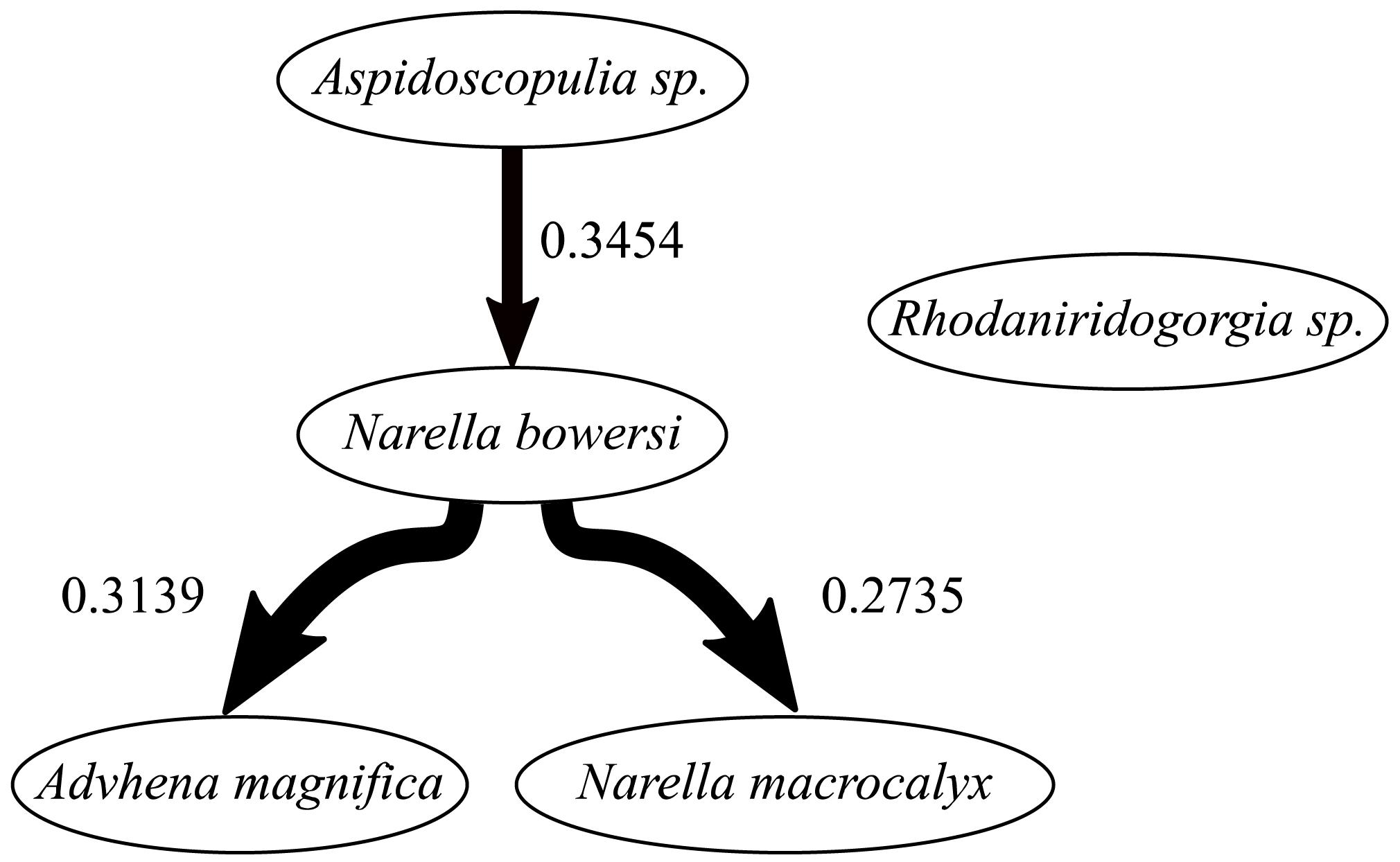
Figure 6. Bayesian networks of associations between abundant sponge and corals. Dependencies between taxa are indicated by the lines connecting the two taxa, the width of which indicates the occurrence rate in the bootstrap analyses (wider lines indicate higher occurrence). Arrows indicate non-mutual dependence between two taxa; A- > B indicates that B depends on A. Mean interaction strengths of the correlations are indicated; positive interaction strengths indicating aggregation, negative interaction strengths indicating segregation. For more details, see section “Materials and Methods.”
The nature of these changes depends on the different biotic and abiotic intra and inter-specific interactions. For this community, the strength of the inter-specific interactions (as calculated by the PCF value; Figure 7) is of similar magnitude to the intra-specific interactions (Figure 5), with the exception of the univariate N. macrocalyx distribution which is significantly more aggregated than the other taxa (Figure 5). The relative strength of the bivariate interactions suggests that the community will be more sensitive to changes in one taxon’s population than a community with only weak bivariate interactions. However, this cascade effect will depend on the nature of each interaction. The habitat association N. bowersi—Aspidoscopulia is a mutual correlation to a third factor, the habitat heterogeneity, and so any community effects may be muted via this mutual factor, making the N. bowersi—Aspidoscopulia interaction more robust than the other two direct biotic interactions. Narella bowersi and Aspidoscopulia share a mutual habitat heterogeneity, which in higher density areas leads to spatial segregation over larger spatial scales (Figure 7A), suggesting a level of competition or thinning out between larger specimens (Getzin et al., 2006). Thus, if the density of Aspidoscopulia was reduced, the inter-specific competition may also be reduced, potentially leading to less thinning and so higher densities of the N. bowersi. Both Advhena and N. macrocalyx have dependencies on N. bowersi, and so these two taxa are likely to be affected by any population changes. The Advhena– N. bowersi interaction was best-modeled by a linked cluster model (Table 5), whereby the Advhena were centered around the N. bowersi. This facilitation was likely due to the Advhena filling the unoccupied space around the N. bowersi, seen in the univariate segregation of the N. bowersi in the Ridge area (Table 4 and Figure 5), and leading to an aggregation of the Advhena around the N. bowersi (Figure 7). The same best-fit link cluster described the bivariate distribution in the Ridge Crest area but with a lower goodness-of-fit (Table 5), suggesting that a weaker version of this effect was occurring there. Therefore, if N. bowersi increases in density, such as via a reduction in Aspidoscopulia, then the effect on Advhena is likely to be positive, due to increased intra-specific N. bowersi competition leading to increased segregation. An increase in N. bowersi may lead to a decrease of N. macrocalyx because an increase in density of N. macrocalyx may increase the strength of the competition in the N. macrocalyx—N. bowersi interaction. The mix of positive and negative biotic interactions coupled to mutual habitat associations is therefore likely to result in a mixture of positive and negative effects on the community in the event of sudden changes and/or mass-mortality events.
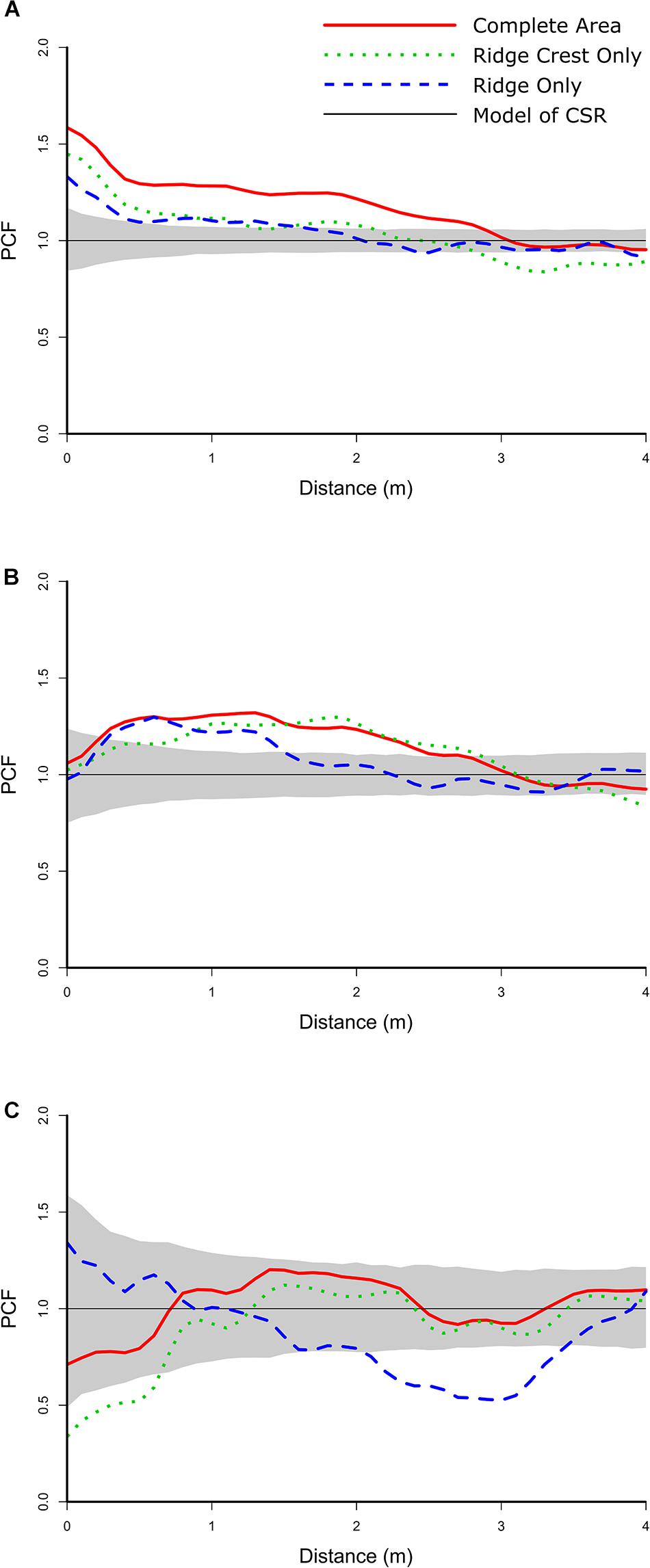
Figure 7. Bivariate PCF analyses for the taxa with non-independent spatial distributions. The gray area is the simulation envelope of complete spatial randomness (CSR) for 999 Monte Carlo simulations. The x-axis is the inter-point distance between organisms in meters. On the y-axis, PCF = 1 indicates CSR and is indicated by a black line, < 1 indicates segregation, and > 1 indicates aggregation. (A) N. bowersi – Aspidoscopulia. (B) N. bowersi – Advhena magnifica. (C) N. bowersi—N. macrocalyx.
To our knowledge, this study is the first to analyze the mortality, population and community dynamics of a deep-sea sponge community using SPPA. Our results provide the first insight into the variety of ecological behaviors within this benthic community, and show how these different organisms have developed diverse responses for the biotic and abiotic gradients within their habitat. We have demonstrated how ecological interactions change with substrate topography, while the community composition remains relatively constant. BNI has demonstrated the connectivity of the abundant taxa, identifying N. bowersi as the most connected taxon, and coupled with SPPA analyses has enabled us to speculate on the possible consequences, both positive and negative, of changes to the community. By identifying and quantifying the strength of abiotic and biotic interactions, these analyses have the potential to identify how different taxa are likely to be affected by different environmental changes. Identification of the crucial factors for different taxa have the potential to be used in management and conservation efforts to help mitigate anthropogenic changes.
The datasets presented in this study can be found in online repositories. The names of the repository/repositories and accession number(s) can be found below: https://doi.org/10.6084/m9.figshare.12284249.
EM conceived this study, processed the 3D model to spatial map, analyzed the data, and wrote the manuscript. SH developed the protocol for creating the 3D model from the video data and reconstructed the 3D model. Both authors contributed to the article and approved the submitted version.
The cruise was supported and conducted by the NOAA Office of Ocean Exploration and Research. Data/imagery courtesy of NOAA’s Office of Ocean Exploration and Research Archives. The analyses was covered by a Natural Environment Research Council Independent Research Fellowship NE/S014756/1 to EM.
The authors declare that the research was conducted in the absence of any commercial or financial relationships that could be construed as a potential conflict of interest.
We wish to thank Chris Kelley both as the lead scientist for the cruise and for his help with the data.
Baddeley, A., Rubak, E., and Møller, J. (2011). Score, pseudo-score and residual diagnostics for spatial point process models. Stat. Sci. 26, 613–646. doi: 10.1214/11-STS367
Baddeley, A., and Turner, R. (2005). Spatstat: a R package for analyzing spatial point patterns. J. Stat. Softw. 12, 1–42.
Baker, K., Snelgrove, P. V. R., Fifield, D. A., Edinger, E., Wareham, V., Haedrich, R. L., et al. (2019). Small-scale patterns in the distribution and condition of bamboo coral, Keratoisis grayi, in Submarine Canyons on the Grand Banks, Newfoundland. Front. Mar. Sci. 6:374. doi: 10.3389/fmars.2019.00374
Beaulieu, S. E. (2001). Colonization of habitat islands in the deep sea: recruitment to glass sponge stalks. Deep Sea Res. Part I Oceanogr. Res. Pap. 48, 1121–1137. doi: 10.1016/S0967-0637(00)00055-8
Beazley, L., Kenchington, E., Yashayaev, I., and Murillo, F. J. (2015). Drivers of epibenthic megafaunal composition in the sponge grounds of the Sackville Spur, northwest Atlantic. Deep Sea Res. Part I Oceanogr. Res. Pap. 98, 102–114. doi: 10.1016/j.dsr.2014.11.016
Beazley, L., Wang, Z., Kenchington, E., Yashayaev, I., Rapp, H. T., Xavier, J. R., et al. (2018). Predicted distribution of the glass sponge Vazella pourtalesi on the Scotian Shelf and its persistence in the face of climatic variability. PLoS One 13:e0205505. doi: 10.1371/journal.pone.0205505
Bell, J. J. (2008). The functional roles of marine sponges. Estuar. Coast. Shelf Sci. 79, 341–353. doi: 10.1016/j.ecss.2008.05.002
Berman, M. (1986). Testing for spatial association between a point process and another stochastic process. J. R. Stat. Soc. Ser. C 35, 54–62. doi: 10.2307/2347865
Besag, J. (1974). Spatial interaction and the statistical analysis of lattice systems. J. R. Stat. Soc. Ser. B 36, 192–225. doi: 10.1111/j.2517-6161.1974.tb00999.x
Buhl-Mortensen, L., Vanreusel, A., Gooday, A. J., Levin, L. A., Priede, I. G., Buhl-Mortensen, P., et al. (2010). Biological structures as a source of habitat heterogeneity and biodiversity on the deep ocean margins. Mar. Ecol. 31, 21–50. doi: 10.1111/j.1439-0485.2010.00359.x
Chu, J. W. F., and Leys, S. P. (2010). High resolution mapping of community structure in three glass sponge reefs (Porifera. Hexactinellida). Mar. Ecol. Prog. Ser. 417, 97–113. doi: 10.3354/meps08794
Clark, M. R., Rowden, A. A., Schlacher, T., Williams, A., Consalvey, M., Stocks, K. I., et al. (2010). The ecology of seamounts: structure, function, and human impacts. Annu. Rev. Mar. Sci. 2, 253–278. doi: 10.1146/annurev-marine-120308-081109
Connell, J. H. (1971). “On the role of natural enemies in preventing competitive exclusion in some marine animals and in rain forest trees,” in Dynamics of Populations: Proceedings of the Advanced Study Institute on Dynamics of Numbers in Populations, eds P. J. den Boer and G. R. Gradwell (Oosterbeek: Wiley), 7–18.
Coppari, M., Gori, A., Viladrich, N., Saponari, L., Canepa, A., Grinyó, J., et al. (2016). The role of Mediterranean sponges in benthic–pelagic coupling processes: Aplysina aerophoba and Axinella polypoides case studies. J. Exp. Mar. Biol. Ecol. 477, 57–68. doi: 10.1016/j.jembe.2016.01.004
Dale, M. R. T., and Fortin, M.-J. (2014). Spatial Analysis: A Guide For Ecologists. Cambridge: Cambridge University Press.
Dayton, P., Jarrell, S., Kim, S., Thrush, S., Hammerstrom, K., Slattery, M., et al. (2016). Surprising episodic recruitment and growth of Antarctic sponges: implications for ecological resilience. J. Exp. Mar. Biol. Ecol. 482, 38–55. doi: 10.1016/j.jembe.2016.05.001
Dayton, P. K. (1971). Competition, disturbance, and community organization: the provision and subsequent utilization of space in a rocky intertidal community. Ecol. Monogr. 41, 351–389. doi: 10.2307/1948498
Dayton, P. K. (1972). “Toward an understanding of community resilience and the potential effects of enrichments to the benthos at McMurdo Sound, Antarctica,” in Proceedings of the Colloquium on Conservation Problems in Antarctica, Blacksberg, VA, 81–96.
Dayton, P. K. (1989). Interdecadal Variation in an Antarctic Sponge and Its Predators from Oceanographic Climate Shifts. Science 245, 1484–1486. doi: 10.1126/science.245.4925.1484
Dayton, P. K., Kim, S., Jarrell, S. C., Oliver, J. S., Hammerstrom, K., Fisher, J. L., et al. (2013). Recruitment, Growth and Mortality of an Antarctic Hexactinellid Sponge, Anoxycalyx joubini. PLoS One 8:e56939. doi: 10.1371/journal.pone.0056939
Deignan, L. K., and Pawlik, J. R. (2015). Perilous proximity: Does the Janzen–Connell hypothesis explain the distribution of giant barrel sponges on a Florida coral reef? Coral Reefs 34, 561–567. doi: 10.1007/s00338-014-1255-x
Di Camillo, C. G., and Cerrano, C. (2015). Mass mortality events in the NW Adriatic Sea: phase Shift from Slow- to Fast-Growing Organisms. PLoS One 10:e0126689. doi: 10.1371/journal.pone.0126689
Dickie, I. A., Schnitzer, S. A., Reich, P. B., and Hobbie, S. E. (2005). Spatially disjunct effects of co-occurring competition and facilitation. Ecol. Lett. 8, 1191–1200. doi: 10.1111/j.1461-0248.2005.00822.x
Diggle, P. J., Ribeiro, P. J., and Christensen, O. F. (2003). “An introduction to model-based geostatistics,” in Spatial statistics and computational methods, (New York, NY: Springer), 43–86.
Diggle, P., Zheng, P., and Durr, P. (2005). Nonparametric estimation of spatial segregation in a multivariate point process: bovine tuberculosis in Cornwall, UK. J. R. Stat. Soc. Ser. C 54, 645–658. doi: 10.1111/j.1467-9876.2005.05373.x
Dunham, A., Archer, S. K., Davies, S. C., Burke, L. A., Mossman, J., Pegg, J. R., et al. (2018). Assessing condition and ecological role of deep-water biogenic habitats: glass sponge reefs in the Salish Sea. Mar. Environ. Res. 141, 88–99. doi: 10.1016/j.marenvres.2018.08.002
Durden, J. M., Bett, B. J., and Ruhl, H. A. (2015). The hemisessile lifestyle and feeding strategies of Iosactis vagabunda (Actiniaria, Iosactiidae), a dominant megafaunal species of the Porcupine Abyssal Plain. Deep Sea Res. Part I Oceanogr. Res. Pap. 102, 72–77. doi: 10.1016/j.dsr.2015.04.010
Easson, C. G., Slattery, M., Baker, D. M., and Gochfeld, D. J. (2014). Complex ecological associations: competition and facilitation in a sponge–algal interaction. Mar. Ecol. Prog. Ser. 507, 153–167. doi: 10.3354/meps10852
Easson, C. G., Slattery, M., Momm, H. G., Olson, J. B., Thacker, R. W., and Gochfeld, D. J. (2013). Exploring individual- to population-level impacts of disease on coral reef sponges: using spatial analysis to assess the fate, dynamics, and Transmission of Aplysina Red Band Syndrome (ARBS). PLoS One 8:e79976. doi: 10.1371/journal.pone.0079976
Fraley, C., Raftery, A. E., Murphy, T. B., and Scrucca, L. (2012). mclust version 4 for R: normal mixture modeling for model-based clustering, classification, and density estimation. Technical Report No. 597, Department of Statistics, University of Washington.
Genin, A., Dayton, P. K., Lonsdale, P. F., and Spiess, F. N. (1986). Corals on seamount peaks provide evidence of current acceleration over deep-sea topography. Nature 322, 59–61. doi: 10.1038/322059a0
Getzin, S., Dean, C., He, F., Trofymow, J. A., Wiegand, K., and Wiegand, T. (2006). Spatial patterns and competition of tree species in a Douglas-fir chronosequence on Vancouver Island. Ecography 29, 671–682. doi: 10.1111/j.2006.0906-7590.04675.x
Getzin, S., Nuske, R. S., and Wiegand, K. (2014). Using Unmanned Aerial Vehicles (UAV) to Quantify Spatial Gap Patterns in Forests. Remote Sens. 6, 6988–7004. doi: 10.3390/rs6086988
Gibbs, D. A., and Hay, M. E. (2015). Spatial patterns of coral survivorship: impacts of adult proximity versus other drivers of localized mortality. PeerJ 3:e1440. doi: 10.7717/peerj.1440
Hawkes, N., Korabik, M., Beazley, L., Rapp, H. T., Xavier, J. R., and Kenchington, E. (2019). Glass sponge grounds on the Scotian Shelf and their associated biodiversity. Mar. Ecol. Prog. Ser. 614, 91–109. doi: 10.3354/meps12903
Heckerman, D., Geiger, D., and Chickering, D. M. (1995). Learning Bayesian networks: the combination of knowledge and statistical data. Mach. Learn. 20, 197–243. doi: 10.1007/BF00994016
Hourigan, T. F., Kelley, C., McGuinn, R., Bingo, S., Moriwake, V. C., Putts, M., et al. (2020). Forests of the Deep: High-Density Deep-Sea Coral and Sponge Communities in the Central and Western Pacific. Ocean Sciences Meeting 2020. Washington, DC: American Geophysical Union.
Howell, K.-L., Piechaud, N., Downie, A.-L., and Kenny, A. (2016). The distribution of deep-sea sponge aggregations in the North Atlantic and implications for their effective spatial management. Deep Sea Res. Part I Oceanogr. Res. Pap. 115, 309–320. doi: 10.1016/j.dsr.2016.07.005
Illian, J., Penttinen, A., Stoyan, H., and Stoyan, D. (2008). Statistical Analysis and Modelling of Spatial Point Patterns. Vol. 70, John Wiley & Sons.
Janzen, D. H. (1970). Herbivores and the Number of Tree Species in Tropical Forests. Am. Nat. 104, 501–528. doi: 10.1086/282687
Jolles, A. E., Sullivan, P., Alker, A. P., and Harvell, C. D. (2002). Disease transmission of Aspergillosis in sea fans: inferring process from spatial pattern. Ecology 83, 2373–2378.
Jones, S. P. (2003). Haskell 98 Language and Libraries: The Revised Report. Cambridge: Cambridge University Press.
Kahn, A. S., Yahel, G., Chu, J. W. F., Tunnicliffe, V., and Leys, S. P. (2015). Benthic grazing and carbon sequestration by deep-water glass sponge reefs. Limnol. Oceanogr. 60, 78–88. doi: 10.1002/lno.10002
Kazanidis, G., Henry, L.-A., Roberts, J. M., and Witte, U. F. M. (2016). Biodiversity of Spongosorites coralliophaga (Stephens, 1915) on coral rubble at two contrasting cold-water coral reef settings. Coral Reefs 35, 193–208. doi: 10.1007/s00338-015-1355-2
Kelley, C., Elliott, K., and Malik, M. (2018). Okeanos Explorer ROV Dive Summary Dive 11 [Dive Summary]. Available online at: https://catalog.data.gov/dataset/ex1706-dive11-ancillary-data-collection-including-reports-kmls-spreadsheets-and-data (accessed September 5, 2020).
Kenchington, E., Power, D., and Koen-Alonso, M. (2013). Associations of demersal fish with sponge grounds on the continental slopes of the northwest Atlantic. Mar. Ecol. Prog. Ser. 477, 217–230. doi: 10.3354/meps10127
Kennedy, B. R. C., Cantwell, K., Malik, M., Kelley, C., Potter, J., Elliott, K., et al. (2019). The unknown and the unexplored: insights into the Pacific Deep-Sea Following NOAA CAPSTONE Expeditions. Front. Mar. Sci. 6:480. doi: 10.3389/fmars.2019.00480
Knudby, A., Kenchington, E., and Murillo, F. J. (2013). Modeling the distribution of geodia sponges and sponge grounds in the Northwest Atlantic. PLoS One 8:e82306. doi: 10.1371/journal.pone.0082306
Law, R., Illian, J., Burslem, D. F. R. P., Gratzer, G., Gunatilleke, C. V. S., and Gunatilleke, I. A. U. N. (2009). Ecological information from spatial patterns of plants: insights from point process theory. J. Ecol. 97, 616–628. doi: 10.1111/j.1365-2745.2009.01510.x
Levin, S. A. (1992). The Problem of Pattern and Scale in Ecology: the Robert H. MacArthur Award Lecture. Ecology 73, 1943–1967.
Liang, Y., Guo, L.-D., Du, X.-J., and Ma, K.-P. (2007). Spatial structure and diversity of woody plants and ectomycorrhizal fungus sporocarps in a natural subtropical forest. Mycorrhiza 17, 271–278. doi: 10.1007/s00572-006-0096-z
Lin, Y.-C., Chang, L.-W., Yang, K.-C., Wang, H.-H., and Sun, I.-F. (2011). Point patterns of tree distribution determined by habitat heterogeneity and dispersal limitation. Oecologia 165, 175–184. doi: 10.1007/s00442-010-1718-x
Lingua, E., Cherubini, P., Motta, R., and Nola, P. (2008). Spatial structure along an altitudinal gradient in the Italian central Alps suggests competition and facilitation among coniferous species. J. Veg. Sci. 19, 425–436. doi: 10.3170/2008-8-18391
Loosmore, N. B., and Ford, E. D. (2006). Statistical Inference Using the G or K Point Pattern Spatial Statistics. Ecology 87, 1925–1931.
Lundsten, L., Barry, J. P., Cailliet, G. M., Clague, D. A., DeVogelaere, A. P., and Geller, J. B. (2009). Benthic invertebrate communities on three seamounts off southern and central California, USA. Mar. Ecol. Prog. Ser. 374, 23–32. doi: 10.3354/meps07745
Luter, H. M., Bannister, R. J., Whalan, S., Kutti, T., Pineda, M.-C., and Webster, N. S. (2017). Microbiome analysis of a disease affecting the deep-sea sponge Geodia barretti. FEMS Microbiol. Ecol. 93:fix074. doi: 10.1093/femsec/fix074
Luter, H. M., and Webster, N. S. (2017). “Sponge Disease and Climate Change,” in Climate Change, Ocean Acidification and Sponges: Impacts Across Multiple Levels of Organization, eds J. L. Carballo and J. J. Bell (Berlin: Springer), 411–428. doi: 10.1007/978-3-319-59008-0_9
Maldonado, M., Aguilar, R., Bannister, R. J., Bell, J. J., Conway, K. W., Dayton, P. K., et al. (2017). “Sponge grounds as key marine habitats: a synthetic review of types, structure, functional roles, and conservation concerns,” in Marine Animal Forests: The Ecology of Benthic Biodiversity Hotspots, eds S. Rossi, L. Bramanti, A. Gori, and C. Orejas Saco del Valle (Cham: Springer). doi: 10.1007/978-3-319-17001-5_24-1
Malik, M., Jerram, K., Wilkins, C., and Baechler, N. (2018). Mapping Data Acquisition and Processing Summary Report Cruise. EX-17-06: Laulima O Ka Moana Exploring Deep MonumentWaters Around Johnston Atoll (ROV/Mapping). Available online at: https://repository.library.noaa.gov/view/noaa/21365 (accessed September 5, 2020).
McClain, C., and Barry, J. P. (2010). Habitat heterogeneity, disturbance, and productivity work in concert to regulate biodiversity in deep submarine canyons. Ecology 91, 964–976.
McClain, C. R., Lundsten, L., Ream, M., Barry, J., and DeVogelaere, A. (2009). Endemicity, biogeography, composition, and community structure on a Northeast Pacific Seamount. PLoS One 4:e4141. doi: 10.1371/journal.pone.0004141
McIntire, E. J. B., and Fajardo, A. (2009). Beyond description: the active and effective way to infer processes from spatial patterns. Ecology 90, 46–56. doi: 10.1890/07-2096.1
Meyer, H. K., Roberts, E. M., Rapp, H. T., and Davies, A. J. (2019). Spatial patterns of arctic sponge ground fauna and demersal fish are detectable in autonomous underwater vehicle (AUV) imagery. Deep Sea Res. Part I Oceanogr. Res. Pap. 153:103137. doi: 10.1016/j.dsr.2019.103137
Milns, I., Beale, C. M., and Smith, V. A. (2010). Revealing ecological networks using Bayesian network inference algorithms. Ecology 91, 1892–1899. doi: 10.1890/09-0731.1
Mitchell, E. G. (2011). Functional programming through deep time: modeling the first complex ecosystems on earth. ACM SIGPLAN Notices 46, 28–31. doi: 10.1145/2034574.2034779
Mitchell, E. G., and Butterfield, N. J. (2018). Spatial analyses of Ediacaran communities at Mistaken Point. Paleobiology 44, 40–57. doi: 10.1017/pab.2017.35
Mitchell, E. G., Durden, J. M., and Ruhl, H. A. (2020a). First network analysis of interspecific associations of abyssal benthic megafauna reveals potential vulnerability of abyssal hill community. Prog. Oceanogr. 187:102401. doi: 10.1016/j.pocean.2020.102401
Mitchell, E. G., Harris, S., Kenchington, C. G., Vixseboxse, P., Roberts, L., Clark, C., et al. (2019). The importance of neutral over niche processes in structuring Ediacaran early animal communities. Ecol. Lett. 22, 2028–2038. doi: 10.1111/ele.13383
Mitchell, E. G., and Kenchington, C. G. (2018). The utility of height for the Ediacaran organisms of Mistaken Point. Nat. Ecol. Evol. 2, 1218–1222. doi: 10.1038/s41559-018-0591-6
Mitchell, E. G., Kenchington, C. G., Harris, S., and Wilby, P. R. (2018). Revealing rangeomorph species characters using spatial analyses. Can. J. Earth Sci. 55, 1262–1270. doi: 10.1139/cjes-2018-0034
Mitchell, E. G., Kenchington, C. G., Liu, A. G., Matthews, J. J., and Butterfield, N. J. (2015). Reconstructing the reproductive mode of an Ediacaran macro-organism. Nature 524, 343–346. doi: 10.1038/nature14646
Mitchell, E. G., and Whittle, R. Huw Griffths (2020b). Investigating benthic ecosystem cascade effects in Antarctica using Bayesian network inference. Commun. Biol. doi: 10.1038/s42003-020-01310-8
Muko, S., Shimatani, I. K., and Nozawa, Y. (2014). Spatial analyses for nonoverlapping objects with size variations and their application to coral communities. J. Anim. Ecol. 83, 980–990. doi: 10.1111/1365-2656.12193
Muller, E. M., and van Woesik, R. (2012). Caribbean coral diseases: Primary transmission or secondary infection? Glob. Change Biol. 18, 3529–3535. doi: 10.1111/gcb.12019
Murillo, F. J., Kenchington, E., Koen-Alonso, M., Guijarro, J., Kenchington, T. J., Sacau, M., et al. (2020). Mapping benthic ecological diversity and interactions with bottom-contact fishing on the Flemish Cap (northwest Atlantic). Ecol. Indic. 112:106135. doi: 10.1016/j.ecolind.2020.106135
NOAA Office of Ocean Exploration and Research (n.d.). NOAA Office of Ocean Exploration and Research Benthic Deepwater Animal Identification Guide. Available online at: http://oceanexplorer.noaa.gov/okeanos/animal_guide/animal_guide.htm
Pélissier, R., and Goreaud, F. (2001). A practical approach to the study of spatial structure in simple cases of heterogeneous vegetation. J. Veg. Sci. 12, 99–108. doi: 10.1111/j.1654-1103.2001.tb02621.x
Piazza, P., Gattone, S. A., Guzzi, A., and Schiaparelli, S. (2020). Towards a robust baseline for long-term monitoring of Antarctic coastal benthos. Hydrobiologia 847, 1753–1771. doi: 10.1007/s10750-020-04177-2
Pile, A. J., and Young, C. M. (2006). The natural diet of a hexactinellid sponge: benthic–pelagic coupling in a deep-sea microbial food web. Deep Sea Res. Part I Oceanogr. Res. Pap. 53, 1148–1156. doi: 10.1016/j.dsr.2006.03.008
Prado, E., Sánchez, F., Rodríguez-Basalo, A., Altuna, Á., and Cobo, A. (2019). Analysis of the population structure of a gorgonian forest (Placogorgia sp.) using a photogrammetric 3D modeling approach at Le Danois Bank, Cantabrian Sea. Deep Sea Res. Part I Oceanogr. Res. Pap. 153, 103124. doi: 10.1016/j.dsr.2019.103124
Price, D., Robert, K., Callaway, A., Iacono, C. L., Hall, R., and Huvenne, V. A. I. (2019). Using 3D photogrammetry from ROV video to quantify cold-water coral reef structural complexity and investigate its influence on biodiversity and community assemblage | SpringerLink. Coral Reefs 38, 1007–1021.
R Core Team (2017). R: A Language and Environment for Statistical Computing. Vienna: R Foundation for Statistical Computing.
Raventós, J., Wiegand, T., and Luis, M. D. (2010). Evidence for the spatial segregation hypothesis: a test with nine-year survivorship data in a Mediterranean shrubland. Ecology 91, 2110–2120. doi: 10.1890/09-0385.1
Reiswig, H. M. (1974). Water transport, respiration and energetics of three tropical marine sponges. J. Exp. Mar. Biol. Ecol. 14, 231–249. doi: 10.1016/0022-0981(74)90005-7
Richer de Forges, B., Koslow, J. A., and Poore, G. C. B. (2000). Diversity and endemism of the benthic seamount fauna in the southwest Pacific. Nature 405, 944–947. doi: 10.1038/35016066
Robert, K., Huvenne, V. A. I., Georgiopoulou, A., Jones, D. O. B., Marsh, L., D. O. Carter, G., et al. (2017). New approaches to high-resolution mapping of marine vertical structures. Sci. Rep. 7:9005. doi: 10.1038/s41598-017-09382-z
Robert, K., Jones, D. O. B., Georgiopoulou, A., and Huvenne, V. A. I. (2020). Cold-water coral assemblages on vertical walls from the Northeast Atlantic. Divers. Distrib. 26, 284–298. doi: 10.1111/ddi.13011
Rossi, S., Bramanti, L., Gori, A., and Orejas, C. (2017). “An Overview of the Animal Forests of the World,” in Marine Animal Forests, eds S. Rossi, L. Bramanti, A. Gori, and C. Orejas (Berlin: Springer), 1–26. doi: 10.1007/978-3-319-17001-5_1-1
Rowden, A. A., Schlacher, T. A., Williams, A., Clark, M. R., Stewart, R., Althaus, F., et al. (2010). A test of the seamount oasis hypothesis: seamounts support higher epibenthic megafaunal biomass than adjacent slopes. Mar. Ecol. 31, 95–106. doi: 10.1111/j.1439-0485.2010.00369.x
Samadi, S., Bottan, L., Macpherson, E., De Forges, B. R., and Boisselier, M.-C. (2006). Seamount endemism questioned by the geographic distribution and population genetic structure of marine invertebrates. Mar. Biol. 149, 1463–1475. doi: 10.1007/s00227-006-0306-4
Seidler, T. G., and Plotkin, J. B. (2006). Seed dispersal and spatial pattern in tropical trees. PLoS Biol. 4:e344. doi: 10.1371/journal.pbio.0040344
Smith, V. A., Yu, J., Smulders, T. V., Hartemink, A. J., and Jarvis, E. D. (2006). Computational inference of neural information flow networks. PLoS Comput. Biol. 2:e161. doi: 10.1371/journal.pcbi.0020161
Vieira, R. P., Bett, B. J., Jones, D. O. B., Durden, J. M., Morris, K. J., Cunha, M. R., et al. (2020). Deep-sea sponge aggregations (Pheronema carpenteri) in the Porcupine Seabight (NE Atlantic) potentially degraded by demersal fishing. Prog. Oceanogr. 183:102189. doi: 10.1016/j.pocean.2019.102189
Waagepetersen. (2009). Two-step estimation for inhomogeneous spatial point processes. J. R. Stat. Soc. Ser. B 71, 685–702.
Wang, Y., Camarero, J. J., Luo, T., and Liang, E. (2012). Spatial patterns of Smith fir alpine treelines on the south-eastern Tibetan Plateau support that contingent local conditions drive recent treeline patterns. Plant Ecol. Divers. 5, 311–321. doi: 10.1080/17550874.2012.704647
Webster, N. S. (2007). Sponge disease: A global threat? Environ. Microbiol. 9, 1363–1375. doi: 10.1111/j.1462-2920.2007.01303.x
Wiegand, T., Gunatilleke, S., and Gunatilleke, N. (2007a). Species Associations in a Heterogeneous Sri Lankan Dipterocarp Forest. Am. Nat. 170, E77–E95. doi: 10.1086/521240
Wiegand, T., Kissling, W. D., Cipriotti, P. A., and Aguiar, M. R. (2006). Extending point pattern analysis for objects of finite size and irregular shape. J. Ecol. 94, 825–837. doi: 10.1111/j.1365-2745.2006.01113.x
Wiegand, T., and Moloney, K. A. (2004). Rings, circles, and null-models for point pattern analysis in ecology. Oikos 104, 209–229. doi: 10.1111/j.0030-1299.2004.12497.x
Wiegand, T., and Moloney, K. A. (2013). Handbook of Spatial Point-Pattern Analysis in Ecology. Boca Raton, FL: CRC Press.
Wiegand, T., Moloney, K. A., Naves, J., and Knauer, F. (1999). Finding the missing link between landscape structure and population dynamics: a spatially explicit perspective. Am. Nat. 154, 605–627. doi: 10.1086/303272
Wiegand, T., Wiegand, K., and Getzin, S. (2007b). Analyzing the spatial structure of a Sri Lankan tree species with multiple scales of clustering. Ecology 88, 3088–3102.
Wulff, J. L. (2007). Disease prevalence and population density over time in three common Caribbean coral reef sponge species. J. Mar. Biol. Assoc. U.K. 87, 1715–1720. doi: 10.1017/S002531540705881X
Yu, J. (2005). Developing Bayesian Network Inference Algorithms to Predict Causal Functional Pathways in Biological Systems. Ph.D. thesis, Duke University, Durham.
Yu, J., Smith, V. A., Wang, P. P., Hartemink, E. J., and Jarvis, E. D. (2002). “Using bayesian network inference algorithms to recover molecular genetic regulatory networks,” in Proceedings of the 3rd International Conference on System Biology, Paris.
Keywords: sponges, benthic ecology, deep-sea ecology, Bayesian network inference, community ecology, mortality dynamics, spatial point process analyses, ecological network
Citation: Mitchell EG and Harris S (2020) Mortality, Population and Community Dynamics of the Glass Sponge Dominated Community “The Forest of the Weird” From the Ridge Seamount, Johnston Atoll, Pacific Ocean. Front. Mar. Sci. 7:565171. doi: 10.3389/fmars.2020.565171
Received: 24 May 2020; Accepted: 28 September 2020;
Published: 20 October 2020.
Edited by:
Joana R. Xavier, University of Porto, PortugalReviewed by:
Michael Vecchione, National Oceanic and Atmospheric Administration (NOAA), United StatesCopyright © 2020 Mitchell and Harris. This is an open-access article distributed under the terms of the Creative Commons Attribution License (CC BY). The use, distribution or reproduction in other forums is permitted, provided the original author(s) and the copyright owner(s) are credited and that the original publication in this journal is cited, in accordance with accepted academic practice. No use, distribution or reproduction is permitted which does not comply with these terms.
*Correspondence: Emily G. Mitchell, ZWszMzhAY2FtLmFjLnVr; ZW1pbHlnaG1pdGNoZWxsQGdtYWlsLmNvbQ==
Disclaimer: All claims expressed in this article are solely those of the authors and do not necessarily represent those of their affiliated organizations, or those of the publisher, the editors and the reviewers. Any product that may be evaluated in this article or claim that may be made by its manufacturer is not guaranteed or endorsed by the publisher.
Research integrity at Frontiers
Learn more about the work of our research integrity team to safeguard the quality of each article we publish.