 Matias Scheinin
 Eero Asmala
- 1Department of Environmental Protection, Hanko, Finland
- 2Pro Litore Association, Raseborg, Finland
- 3Tvärminne Zoological Station, Faculty of Biological and Environmental Sciences, University of Helsinki, Hanko, Finland
Productivity and trophic status of aquatic systems is traditionally quantified by chlorophyll a measurements. Environmental conditions and ecological interactions cause variability in chlorophyll a abundance. In coastal ecosystems, shallow and complex bathymetry reduces vertical heterogeneity, but promotes horizontal heterogeneity. However, coastal monitoring programs and scientific surveys are primarily focused on the vertical dimension. Here we demonstrate the spatial patchiness of chlorophyll a in coastal waters. We collected horizontally detailed and extensive in situ chlorophyll a data from the coastal Baltic Sea (SW Finland), covering the ice-free season of an annual cycle. Altogether, more than 200,000 observations were logged by an automated underway measurement system equipped with an optical sensor connected to a flow-through system. We analyzed the spatial heterogeneity of calibrated chlorophyll a data by using multiple statistical approaches, and quantified the chlorophyll a patches using a rolling average filter. We were able to identify patches and quantify their abundance and size for each of the 11 sampling campaigns. On average, 285 patches, ranging from 0.6 to 3142 m in size, were observed on the 830 km sampling transect. The average size of the patches was 237 (95% CI 226–248) m, most patches being between 10 and 1000 m. Our results show that patches of chlorophyll a can be effectively identified and quantified by modern in situ optical instrumentation. Such information is both theoretically and practically relevant. First, these results increase our understanding of the overall heterogeneity of the coastal environment. Further, they demonstrate the value of knowing the magnitude and occurrence of chlorophyll a patchiness in accurate detection of changes in coastal ecosystems caused by increased inputs of nutrients.
Introduction
Understanding environmental change is founded on describing, explaining, and predicting ecosystem state. The trophic state of an ecosystem, or the property of energy availability to its food web (Dodds, 2007), is a fundamental manifestation of ecosystem structure (Scheffer et al., 2001), function (Howarth et al., 2011), and services (Antón et al., 2011). It is thus pertinent for both basic and applied ecology to assess how the trophic state of an ecosystem varies in space and time. Trophic state is typically quantified through total organic carbon, primary producer biomass, or macronutrient availability (Lindeman, 1942; Odum, 1956; Nixon, 1995). Most conventionally, phytoplankton biomass—measured using chlorophyll a concentration (hereafter Chl-a) as a proxy—has been applied as the prime indicator of trophic state (Carlson, 1977).
Ecosystems vary in their trophic state depending primarily on external and internal nutrient fluxes. While external fluxes determine the level of nutrients in an ecosystem, their distribution among its compartments is regulated by internal fluxes, that thus govern how the nutrient level is expressed in the trophic state of the system. External nutrient loading leads to an increase in the trophic state of the recipient ecosystem, that is, eutrophication. Essentially, nutrient enrichment initiates a shift in species composition, which involves concomitant changes in food web structure and ecological transfer efficiency (Havens, 2014). The concrete manifestations of this depend on the rate and degree of eutrophication as well as on ecosystem-specific characteristics. In coastal ecosystems, eutrophication has diminished water clarity, caused toxic algal blooms, resulted in localized hypoxia, and reduced macrovegetation in nearshore environments (Boesch, 2019). In terms of coastal ecosystem services, eutrophication can alter the functioning of the coastal filter, e.g., carbon storage and cross-ecosystem nutrient transfer (Asmala et al., 2017), erosion and pollution control (Barbier et al., 2011), fisheries and nurseries (Worm et al., 2006), as well as the recreational value and aesthetic quality of the environment (Chung et al., 2015). While nutrient loading from point sources has decreased substantially during the past few decades (e.g., Reusch et al., 2018), inputs from diffuse atmospheric and terrestrial sources are difficult to reduce. This difficulty is compounded by the legacy storage of nutrients in soils, waterways and groundwater (Boesch, 2019). Moreover, diffuse loading is challenging to mitigate because of the spatiotemporal heterogeneity of the sources. Consequently, coastal eutrophication is a globally topical problem (Andersen et al., 2019).
In coastal waters, phytoplankton biomass is prone to be patchy due to a combination of environmental, ecological and physiological drivers. Bathymetry, tides, and currents combine freshwater runoff and marine surface and deeper waters over small spatial scales to create considerable spatial complexity in hydrography, mixed layer depth, and nutrient content, driving spatial complexity in phytoplankton biomass. Furthermore, short temporal variability, similar in timescale with that of phytoplankton physiological variability, is induced by advective currents and wind-driven mixing (Carberry et al., 2019). Hence, disregarding the patchiness of Chl-a in assessments of the trophic state of coastal ecosystems is likely to result in spatiotemporally skewed or overgeneralized interpretation of their properties. Robust measurements of Chl-a on adequate scales of space and time are also relevant for planning, prioritizing, targeting, and following up management actions that can alter external nutrient loading.
Quantification of Chl-a patchiness—including the quantity, extent, prevalence, and intensity of the patches—requires sampling with sufficiently high precision and resolution. Two principal sampling approaches are being used: discrete water sampling and in situ observations. Both of these involve their own constraints that complicate the determination of the different patchiness parameters. Discrete water sampling is well suited for the precise quantification of Chl-a, since the pigment can be extracted from the cells and measured reliably and accurately by various methods such as high-performance liquid chromatography (HPLC), spectrophotometry or -fluorometry. However, the quantification of small-scale spatiotemporal variation by discrete sampling is virtually impossible due to the labor-intensity of the approach—resulting in high precision but low resolution (Cloern et al., 1989). By contrast, in situ observations have fewer limitations regarding spatial and temporal resolution. Chl-a can be assessed through in vivo fluorescence from different remote sensing vehicles or waterborne platforms. While these approaches allow for high resolution, their precision is significantly lower with raw values than that of the methods based on chlorophyll a extraction (e.g., Cullen, 1982). The in vivo fluorescence yield per Chl-a may vary depending primarily on the size (Alpine and Cloern, 1985) and species (Proctor and Roesler, 2010) of phytoplankton, and the photochemical (Sosik and Mitchell, 1991) and non-photochemical (Misumi et al., 2016) quenching properties of the species. On top of these proximate causes, the optical complexity of coastal waters in the form of other compounds (e.g., DOM and non-living particles) that fluoresce at similar wavelengths as chlorophyll a will further distort in situ fluorescence measurements. Although in situ observations can be calibrated using discrete water samples, the work is often logistically too challenging due to match up issues (Carberry et al., 2019).
Here, we present a cost-efficient methodological framework that enables the quantification of Chl-a patchiness and its subsequent decomposition into the basic patchiness parameters in heterogeneous coastal waters. Our overall aim was to identify and quantify the chlorophyll a patches, and use these as indicators for patchiness of the coastal environment, in general. The framework builds upon spatially high-frequency Chl-a in situ observations in a geographically complex coastal archipelago environment. To collect the data, we surveyed Chl-a at high resolution in the coastal waters of SW Finland along an 830 km long transect throughout the entire ice-free season of 2019.
Materials and Methods
Study Site and General Description of the Area
The study was carried out within a 40 km by 50 km rectangular area around the SW tip of mainland Finland on both sides of the 60th parallel north and the 23rd meridian east, in the northern Baltic Sea. The area encompasses the entire coastal waters of the cities of Hanko and Raseborg, thus covering parts of the Finnish Archipelago Sea in the west and parts of the Gulf of Finland in the East. The climate of the study area is cold and temperate, or “Dfb” according to the Köppen–Geiger climate classification. The long-term average annual air temperature is 5.3°C, and the average annual rainfall is 603 mm. The sea starts to freeze typically in October, while the ice cover tends to disappear completely in May. However, there are pronounced differences in the prevalence, thickness, and permanence of the ice cover within the area (HELCOM, 2010).
The coastal zone of the northern Baltic Sea exemplifies the heterogeneity of coastal environments, as it is characterized by its vast mosaic-like archipelago consisting of thousands of small islands. Further, littoral zone constitutes a large proportion of these coastal waters due to the planar profile of the region, its fine-scale topographical variability, and the extensive length of the aggregate shoreline. These features translate as comparatively high photic zone coverage as well as strong benthic-pelagic, terrestrial, and atmospheric coupling (McGlathery et al., 2007). While temperature and light modulate phytoplankton dynamics during the ice-free season, primarily nutrient availability and to a lesser extent grazing drive the timing and amount of phytoplankton standing stock biomass, or Chl-a (Lyngsgaard et al., 2017). Further, in shallow and intensively mixed waters phytoplankton production can be very high already before the onset of thermal stratification (Sommer and Lengfellner, 2008). Since nutrients are continuously cycled within the well-mixed system, phytoplankton production is more permanently fueled by the dissolved nutrient resources than in pelagic areas.
Sampling Methods
Flow-Through System Including the Chlorophyll a Sensor
The spatially detailed and extensive in situ Chl-a data were collected by an automated underway measurement system equipped with an optical Chlorophyll a sensor. The system was constructed by Luode Consulting Inc. and installed in a rigid inflatable boat (RIB) (Brig N610H) with 0.4 m draft. The system consisted of seven sequential components as follows: The water intake was placed at 0.5 m depth, facing forward right below the left-hand stern. Since the water intake was the lowest part of the whole system, its minimum operation depth was also 0.5 m. After passing the pump at 29 L/min, the water was led through a lamellar debubbler before entering a 0.5-L cylindrical chamber enclosing an EXO2 sonde equipped with a dual-channel fluorescence sensor (Xylem Inc., United States) for integrated Chl-a detection, incorporating also cyanobacterial contribution by applying two excitation wavelengths; 470 ± 15 and 590 ± 15 nm and one emission detection wavelength at 685 ± 15 nm. From the sonde, the water passed by a faucet for water collection before being led back to the sea from an outflow pipe at the right-hand rail of the boat. Time and GPS position were tracked continuously for geolocating the Chl-a measurements by using an EXO Handheld unit (Xylem Inc., United States) connected to the sonde with a data transmission cable.
Data were constantly recorded at 5 s intervals, while the typical traveling speed of the boat was 22.3 knots (12 m/s), resulting in the vast majority of the data being logged at 60-m intervals. As the spatial resolution of the applied method was determined by the traveling speed of the boat, resolution finer than 60 m could only be achieved at velocities lower than the standard traveling speed at the chosen logging interval. Due to, e.g., complex navigation, marine traffic regulations, or very shallow water depth, the speed of the boat was reduced in few locations. In any given location, traveling speed was virtually invariable among the campaigns, allowing for unbiased temporal comparisons of the patchiness data. In order to maximize the geolocation precision, the total response time of the flow-through system was determined according to Crawford et al. (2015) and adjusted to 10 s by altering the length of the water hose between the water intake and the pump. The total response time consists of the hydraulic lag between the water intake and the cylindrical chamber (8 s), the total exchange of the water in the chamber (0.5 s), and the response time (T63) of the sensor (<2 s).
Sampling Schedule
The samples were collected along an 830 km long transect (Figure 1), where water depth varied between 0.5 and 80 m. The transect was surveyed with 3-week intervals throughout the entire ice-free season from week 14 at the turn of March and April until week 44 at the turn of October and November 2019. However, only a fraction of the transect could be sampled during the first occasion, since sea ice was still covering most of the transect. During all the later occasions, the transect could be followed in high detail so that both the route and the traveling speeds at different parts of the route were virtually constant. Apart from the first sampling occasion, each sampling campaign was carried out during four consecutive days. During each occasion, the number of data points collected was approximately 20,000, totaling 212,150 observations from the eleven sampling occasions. Eight locations were chosen randomly to represent variation in local Chl-a dynamics (Figure 1).
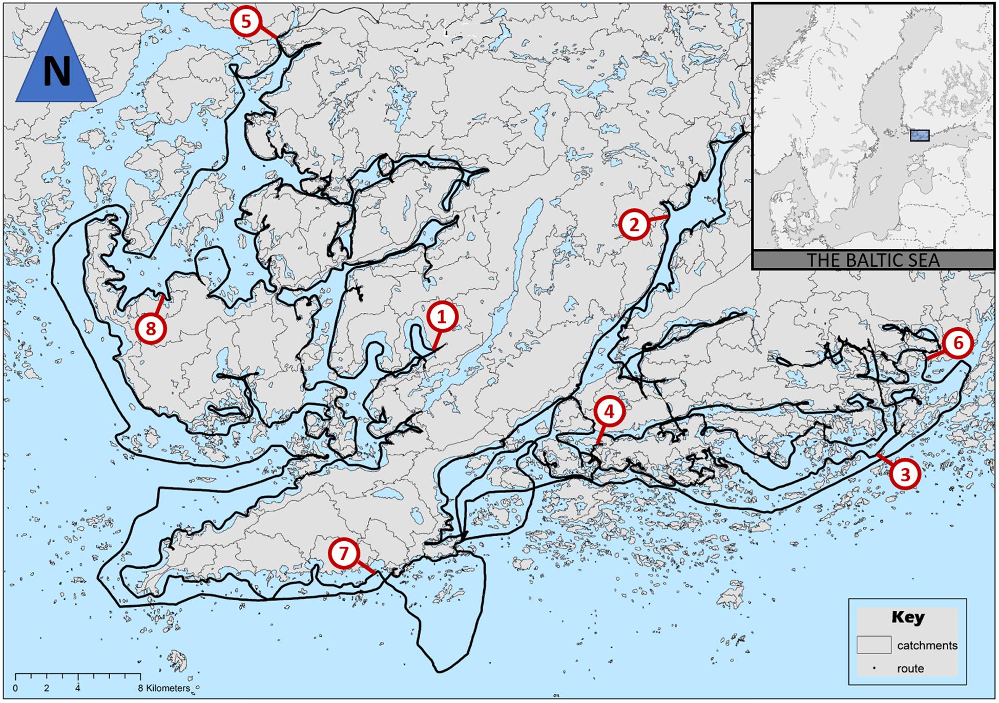
Figure 1. Map of study area with the route of the boat (black solid line) and eight reference stations (1 = Båtviken, 2 = Elimogrundet, 3 = Gästans, 4 = Gyltviken, 5 = Kiskonjoki, 6 = Stakasund, 7 = Stödjekobbarna, 8 = Svärtesviken). Inset figure of the northern Baltic Sea.
Calibration of the in situ Chl-a Observations
During each sampling occasion, 20 discrete water samples were collected for calibrating the in situ Chl-a data. To represent maximal variability in terms of phytoplankton composition and biomass, and of the surrounding conditions, the 20 sampling stations were located along three distinctive environmental gradients, each starting from a river mouth and ending at the open sea. Since the gradients were spatially apart from each other, and each gradient was geographically extensive (12, 18, and 38 km), the collected samples also represented different sampling days and contrasting times of each day. During the brief stop at each sampling station, 50 mL of water was collected into a plastic centrifuge tube from the faucet for water collection while logging parallel Chl-a data. Each sample was immediately filtered onto a GF/F (Whatman) filter. The filter was submerged in ethanol in a glass scintillation vial. The vials were transported in a dark cool box to the laboratory by the end of each sampling day. In the laboratory, the samples were incubated in the dark in a −20°C freezer for 72 h prior to the analysis. The concentration of the extracted Chlorophyll a was determined by fluorometry (Varian Cary Eclipse spectrofluorometer, Agilent, United States) using a plate reader (Simis et al., 2012). Finally, the coefficient of determination between the temporally parallel in situ and extracted Chl-a measurements was calculated by using linear regression with 0 as the intercept (in situ data was validly 0-calibrated). Thus, the slope of the model function was used as the correction factor for the in situ Chl-a data (Supplementary Figure S1).
Data Analysis
We used the calibrated values for the analysis of spatial and temporal variation in Chl-a. Average values for each sampling campaign were calculated, as well as average values for the eight specific locations indicated in Figure 1. Spatial autocorrelation shows the correlation within variables across georeferenced space (Getis, 2008). Although spatial autocorrelation can be used to determine the average size of patches (Sokal and Oden, 1978), autocorrelation occurs over some minimal scale that is dependent on both processes and sampling. Consequently, autocorrelation may not capture patterns smaller than this inherent minimal scale, and other methods to quantify patterns at smaller scales may be needed (Underwood and Chapman, 1996). Autocorrelation (covariance) of the Chl-a observations was calculated for each round separately, up to lag value equaling maximum number of observations for each campaign. We acknowledged the inherent autocorrelation of the high frequency Chl-a observations and used it to identify the large-scale patchiness of Chl-a. Using the sequence of Chl-a observations from each sampling campaign, the difference in Chl-a observations between two sampling points with n number of observations in between was calculated. The difference was calculated for n values of 1–300, which corresponds to 18 km. To complement the autocorrelation analysis and to identify and quantify the local heterogeneity on a smaller scale, we identified patches, i.e., operational units of local heterogeneity by using a rolling mean filter along the sequence of Chl-a observations. This approach allows identification and quantification of local heterogeneity beyond autocorrelation analysis (Underwood and Chapman, 1996). We used the rollapply function from the R package zoo (Zeileis and Grothendieck, 2005) with a rolling bin width of 101 observations (50 observations to both forward and backward from each observation). This corresponded to a distance of 6 m on average, which is approximately four times the size of phytoplankton patches identified by Platt et al. (1970). We applied a threshold of 25%, which means that Chl-a values that deviated (either negatively or positively) more than 25% from the rolling mean value, were categorized as patches. The performance of a range of thresholds and bin widths in patch detection was tested with simulated data, and the combination of threshold value 25% and bin width identified patches from simulated dataset with a 100% accuracy (Supplementary Figure S2). Consecutive observations categorized as patches were assigned a unique patch ID, and the spatial extent of each patch was calculated using the geospatial information of each observation using the R package sf (Pebesma, 2018). The patch extent was determined as the maximum extent, as the distance between the two farthest points of each patch. Paired relationships between average Chl-a, number of patches, and patch extent were analyzed with simple linear regression for each sampling campaign. All statistical analyses were done by using R software (R Core Team, 2014).
Results
The measured Chl-a ranged from 0.76 to 195 μg l–1 during the study period from late March to early November (Figure 2 and Supplementary Figure S3). The overall average was 7.65 μg l–1, but the values varied considerably among sampling campaigns and locations. The lowest average values were observed during the first campaign (4.75 μg l–1), and the highest 3 weeks later, during the second campaign (14.24 μg l–1).
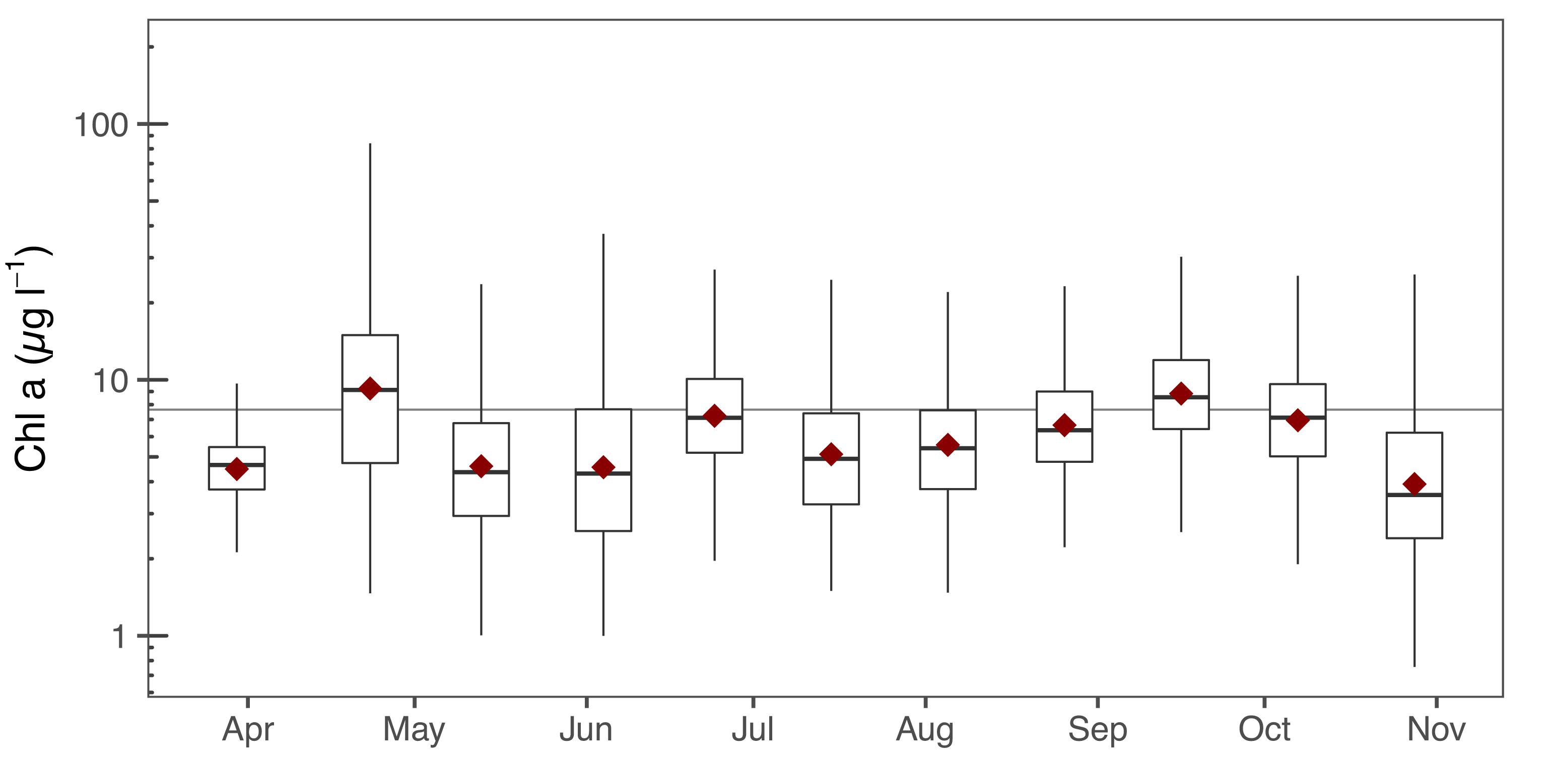
Figure 2. Chl-a during each sampling campaign. Lower and upper ends of boxes indicate the interquartile range (Q3–Q1), whiskers the lowest and the highest values within the range of 1.5 IQR, and thick black line indicates median value. Mean values are indicated by red diamonds, and horizontal line represents the overall mean value across all samplings (7.65 μg l–1). On week 14, the number of observations was only 5514 due to ice cover.
Chl-a varied considerably among the eight randomly chosen sampling points (Figure 3). The lowest values were observed in Stödjekobbarna (3.8 [95% CI 3.6–4.1], range 1.3–7.5 μg l–1), and the highest in Svärtesviken (19.4 [13.9–24.8], 2.2–149.1 μg l–1). The apparent seasonal pattern varied also considerably among the chosen points, and in general, did not follow the overall regional pattern (c.f. Figure 2).
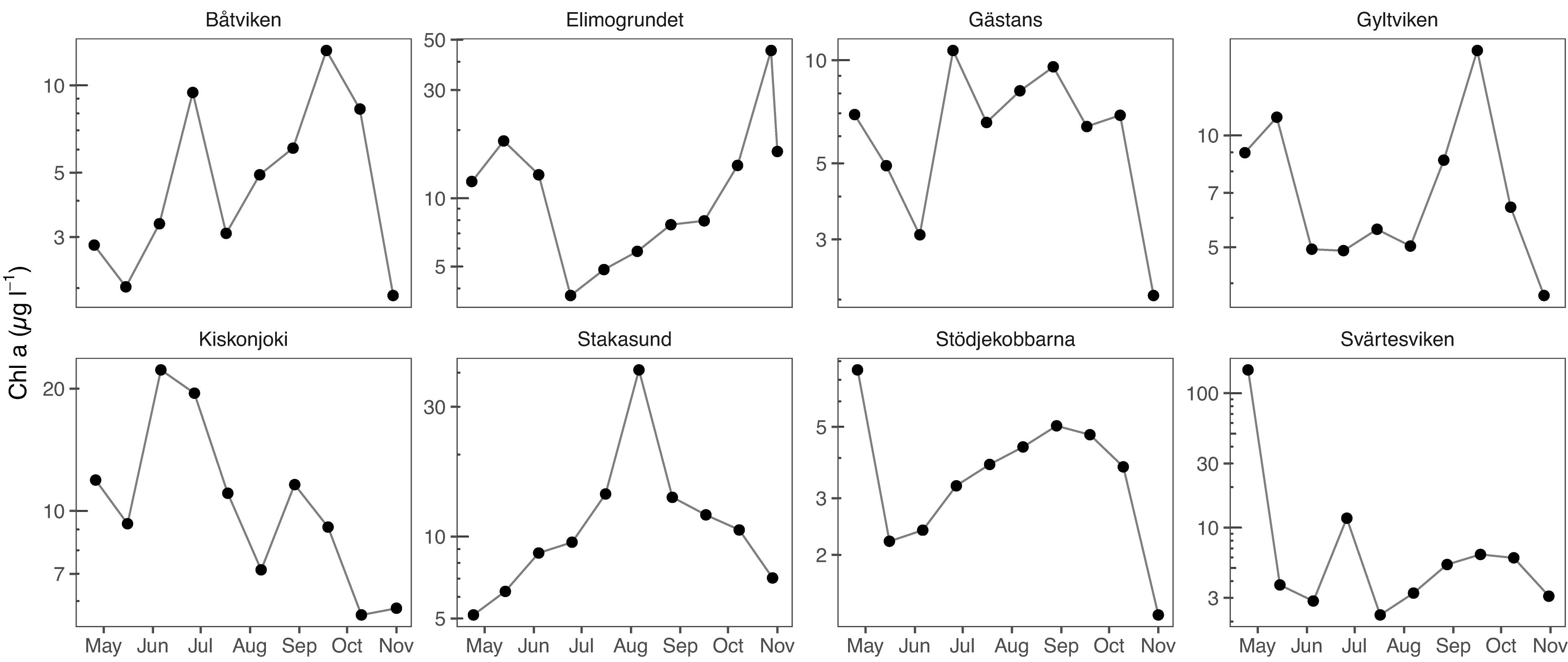
Figure 3. Chl-a at eight randomly selected sampling points, whose locations are indicated in Figure 1. The first sampling campaign (week 14) was not included due to ice cover in most of the points.
Differences in Chl-a among sampling points, i.e., patchiness, varied from one sampling campaign to another (Figure 4). In general, the mean difference between two sampling points increased in concert with the number of observations in between. This increase was not linear, as the difference increase was steepest in the range of ∼<50 observations in between. During the campaign in week 17, the differences were the highest, reaching on average 3.9 (95% CI 3.8–4.0) μg l–1 between two observations that were 300 observations apart. During week 14, the mean difference at an interval of 300 observations was less than 1 μg l–1, as well as during week 20. After week 20, the mean differences gradually increased toward the autumn, reaching 2.8 (2.7–2.9) μg l–1 in week 44.
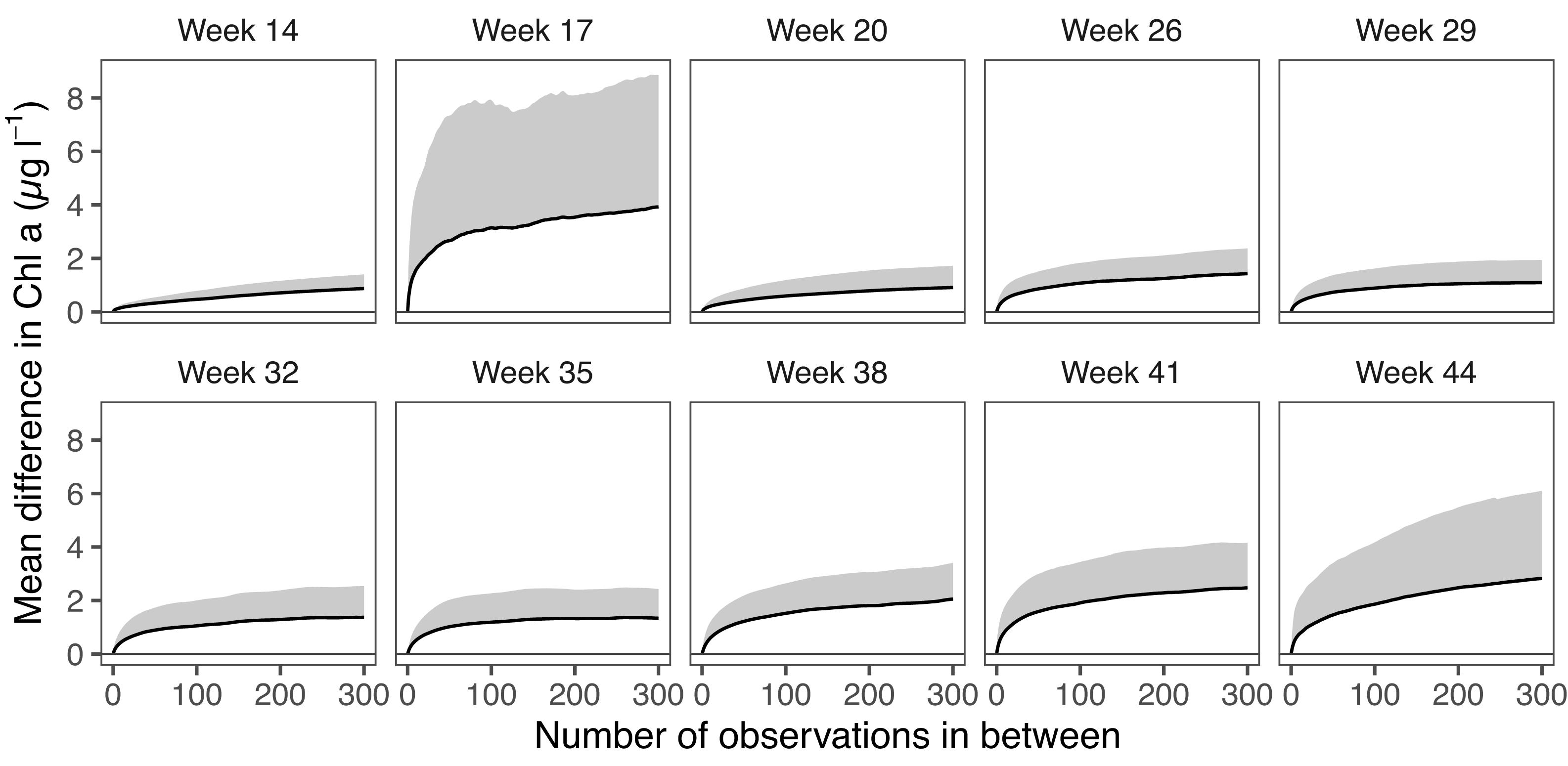
Figure 4. Mean difference in observed Chl-a along a lag gradient, i.e., number of observations between the observations being compared. Gray area indicates 0.65 standard deviation, which corresponds to a 50% confidence interval. Note: week 23 not included.
For the identification of the potential patches in Chl-a observations, we used a rolling mean filter and a deviation threshold, as exemplified in Supplementary Figure S4. By using this approach, we were able to identify multiple patches from each sampling day.
The number of patches varied between the sampling campaigns; from 5 in week 14 and 458 in week 17, and the average number of patches was 285 (Figure 5 and Table 1).
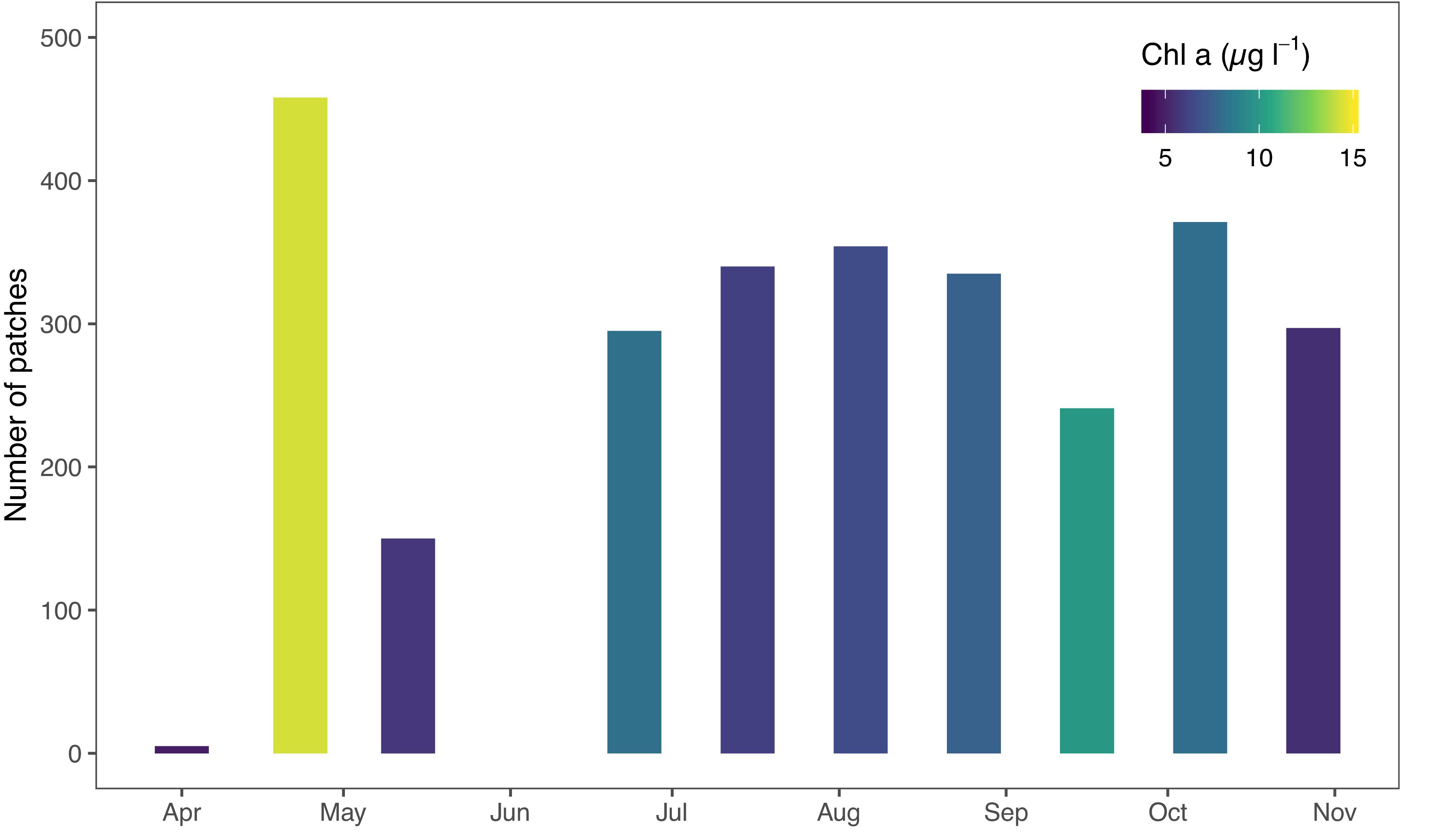
Figure 5. Number of individual patches identified during 10 sampling campaigns. Note that during week 14 the route was limited to offshore areas with only ∼5000 observations. Note: week 23 not included.
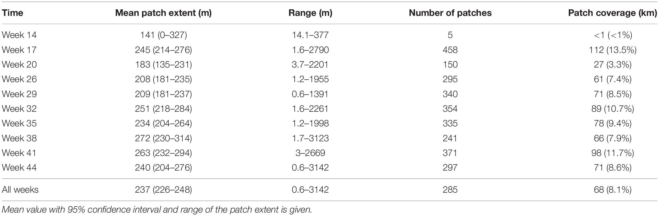
Table 1. Summary statistics of the peak extents during 10 sampling campaigns.
The location of individual patches changed from one sampling to another, appearing apparently randomly across the region (Figure 6). There was a weak positive relationship with average Chl-a and the number of patches during the samplings (p = 0.07).
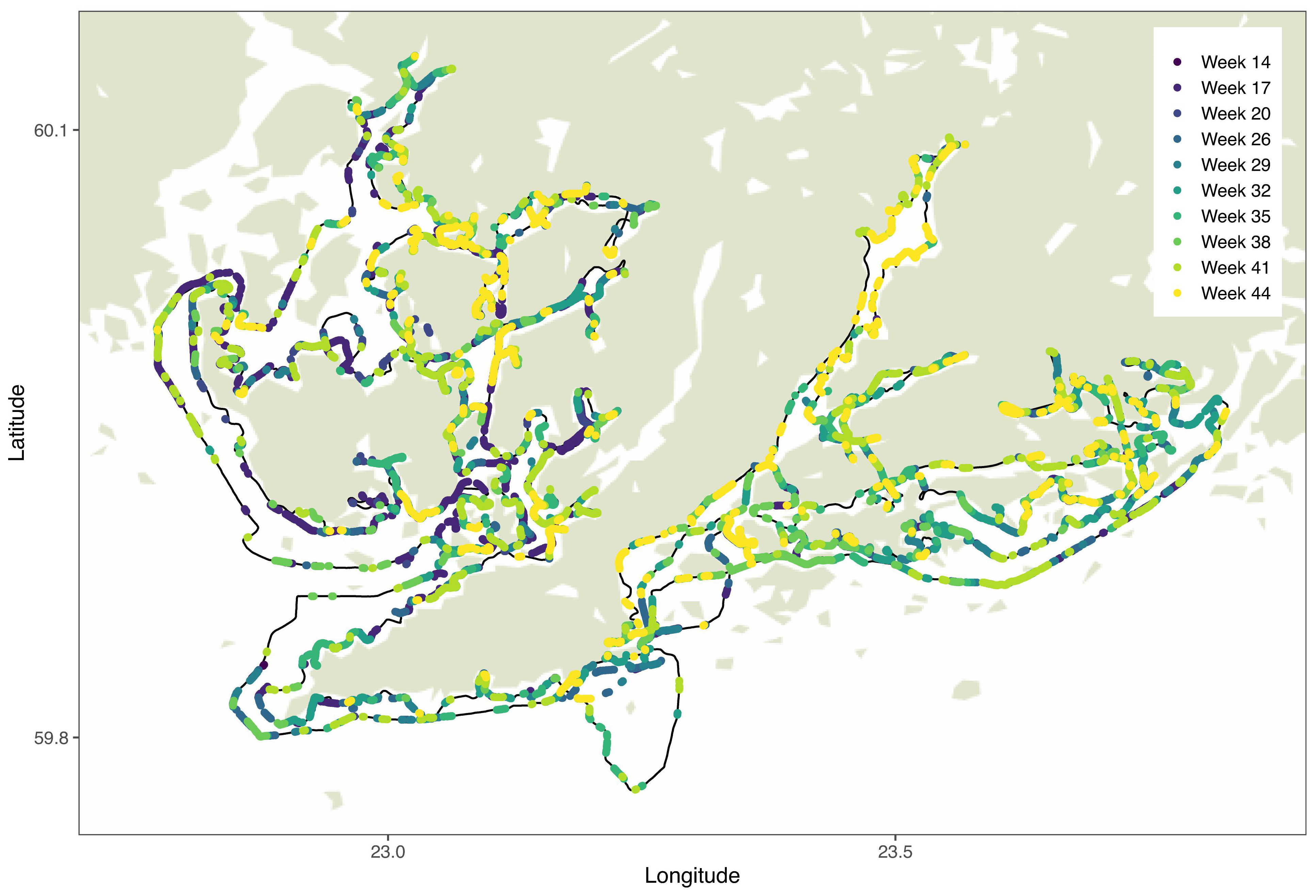
Figure 6. Chl-a patches from each round overlaid on map. Route of the boat marked with black solid line.
Compared to the number of patches, the size of the patches varied less among the sampling occasions, the average values ranging from 141 m in week 14 to 272 m in week 38 (Figure 7). After low patch extent values in week 20 (183 m on average), there was a general increasing trend in patch extents toward autumn. As with the number of patches, patch extent did not have a significant relationship with the average Chl-a of each sampling occasion (p = 0.13).
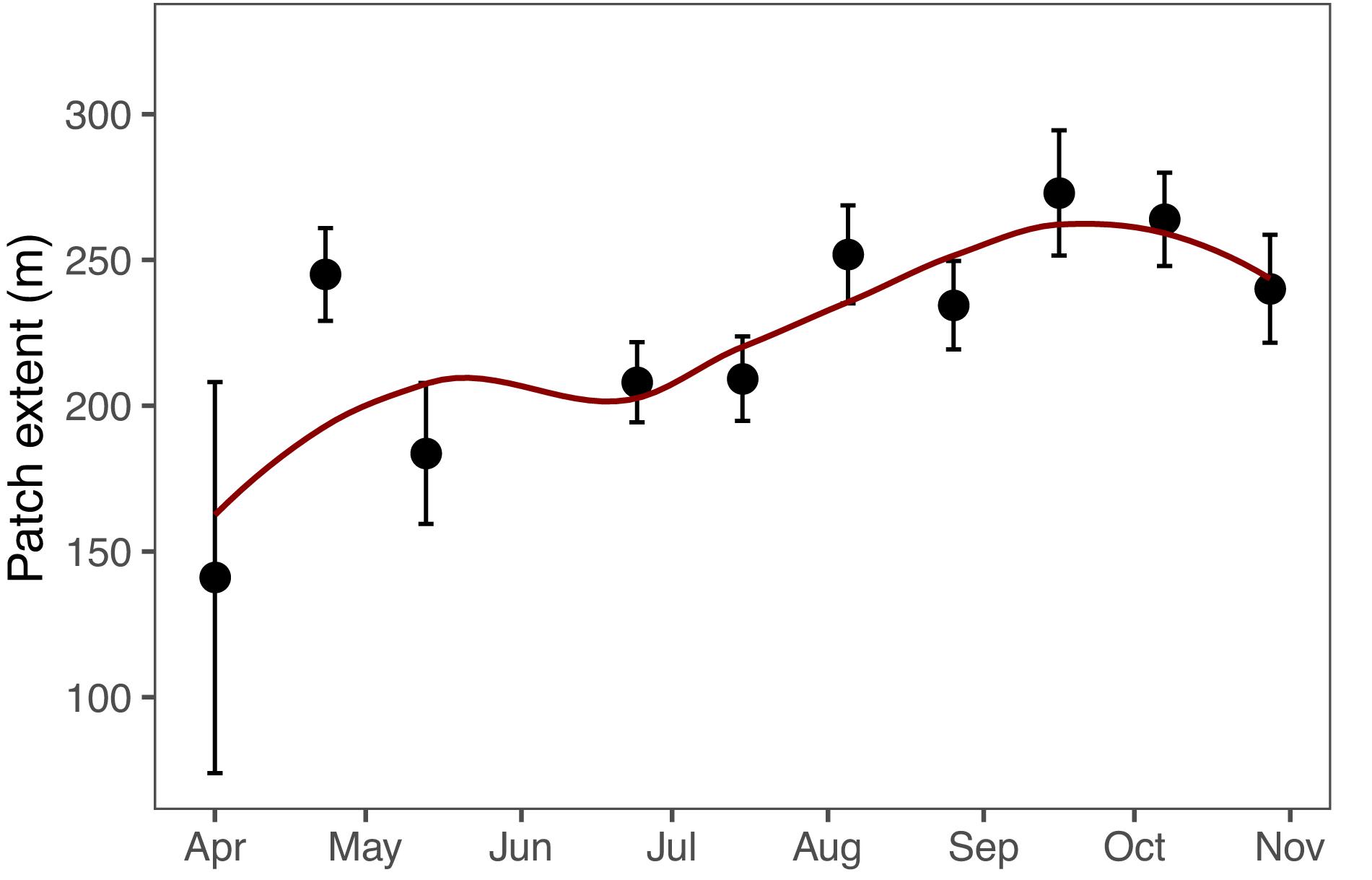
Figure 7. Mean patch extent on each sampling campaign. Error bars indicate ± 1 standard error of mean. Red line indicates locally estimated scatterplot smoothing and gray area 95% confidence interval of the local regression. Note: week 23 not included.
The size of the patches (patch extent) ranged from 0.6 to 3142 m (Figure 8). Most patches were in the range of 10–1000 m, and the modal values between 50 and 100 m.
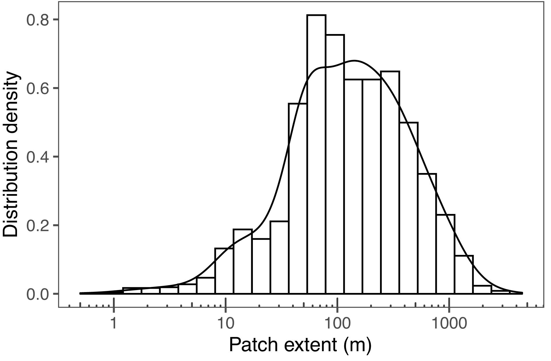
Figure 8. Patch extent distribution density along the size gradient from 0.6 to 3142 m.
Chl-a had weak positive relationship with patch extent (Figure 9A) and number of patches (Figure 9B). The number of patches and the mean patch extent had a significant positive relationship (Figure 9C). In other words, the more patches were observed, the larger they were on average.
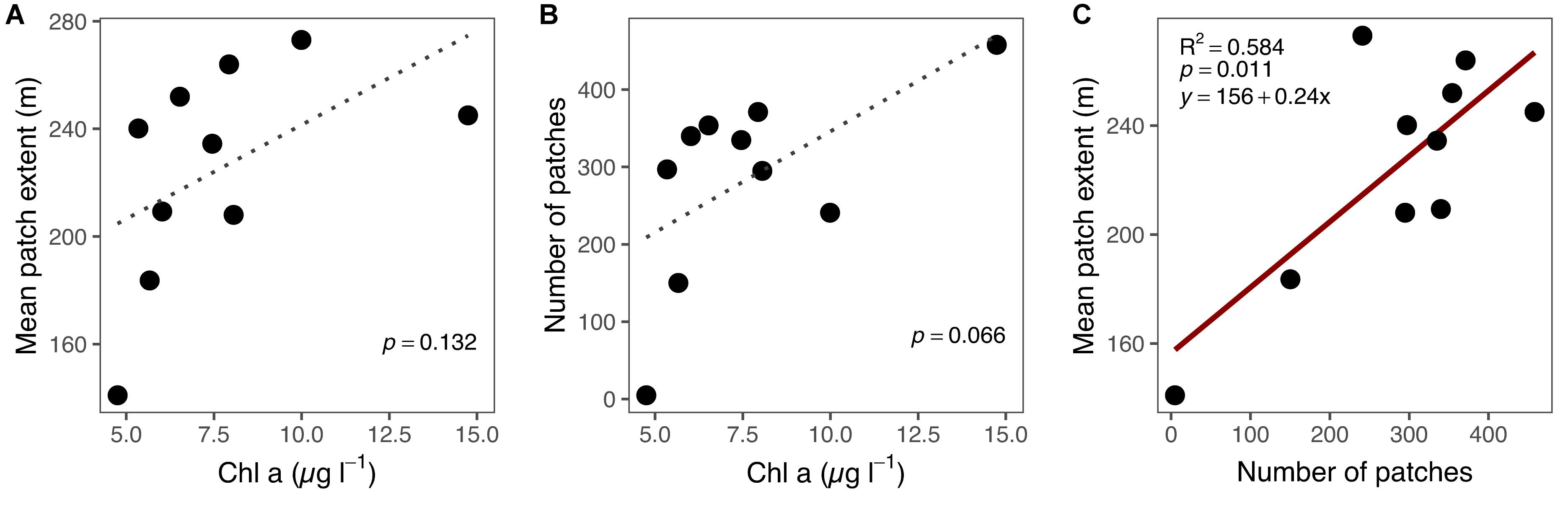
Figure 9. Relationship between (A) Chl a and mean patch extent, (B) Chl a and number of patches and (C) number of patches and mean patch extent for each sampling occasion (week 23 excluded). Red solid line indicates a significant (p < 0.05) linear relationship between variables, and gray dotted line indicates non-significant (p ≥ 0.05).
Discussion
Chlorophyll Concentrations and Phenology
The total average Chl-a across all sampling points and campaigns was 7.65 μg l–1 (Figure 2), which generalizes the eutrophication status of the sampling area to mesotrophic (Carlson, 1977). We observed weak spring and autumn peaks (in April–May and September–October) typical for temperate, pelagic areas (Cebrián and Valiela, 1999; Gasiûnaitë et al., 2005), as well as an apparent unimodal midsummer maximum (July) characteristic for temperate, littoral areas (Harding et al., 2019) from the overall average dynamics of the whole area. The average dynamics appeared relatively static compared to other temperate coastal areas (Carstensen et al., 2015; Harding et al., 2019), since the coastal sampling route averaged and canceled off the seasonality. In other words, the small difference between minima and maxima was simply a manifestation of average dynamics with high variability due to large spatial differences in Chl-a levels and phenology. Annual mean Chl-a levels varied substantially among different locations, while the different locations displayed highly different temporal dynamics (Figure 3). Both sorts of differences are characteristic for nearshore areas and marginal seas, in general (Song et al., 2019). The phenological differences can result from multiple different factors—including the local overall Chl-a level—that affect phytoplankton dynamics. Accordingly, site-specific internal processes, related to their actual trophic state, may change the N:P stoichiometry, overall nutrient availability, or grazing pressure (Sommer et al., 2012). Moreover, especially in the more enclosed areas, temperature and salinity differences are more pronounced and abrupt, driving changes in the temperature- (Yvon-Durocher et al., 2017) or salinity-sensitive (Oseji et al., 2019) parts of the plankton community. Finally, inherent stochasticity can cause spatial heterogeneity in organism and resource distributions, which leads to temporal heterogeneity in resource access for phytoplankton (Anderies and Beisner, 2000).
Chlorophyll Patchiness
Patchiness, here defined as the contrast in Chl-a among different observations as a function of the observation sequence, varied across the year (Figure 4 and Supplementary Figure S5). This applied both to the intensity and scale of patchiness, illustrated by the systematic temporal changes in the level (intensity) and slope (scale) of the mean difference in Chl-a in relation to the observation sequence (Figure 4). The temporal variation in the intensity and scale of patchiness underline that the theoretical and practical implications of patchiness are far from the same around the year. However, the relationship between the intensity and scale of patchiness appeared comparably constant throughout the season, indicating that Chl-a patchiness is a ubiquitous characteristic of coastal waters.
The temporal patterns in the intensity and scale of patchiness may partially be attributed to external nutrient loading. Like in other coastal environments, most of the external nutrient loading in the study area originates from diffuse terrestrial sources (Boesch, 2019). In the spring, high transient loading from diffuse sources is likely to promote considerable horizontal heterogeneity in resource availability, leading to high intensity and scale of patchiness in the distribution of phytoplankton biomass in April (Figure 4). The subsequent collapse in patchiness may be due to, e.g., patch-targeted top-down control of phytoplankton (Sommer et al., 1986) and stochastic dilution by diffusion of the nutrient resources (Romero et al., 2016). During the following months, the considerably decreased but still substantial level of patchiness was maintained probably by the legacy storage of nutrients in the sediments (Vahtera et al., 2007). These sources of internal loading should reflect the diffuse geography of the external ones, while nutrient resuspension rates in shallow and vertically well-mixed waters tend to be driven by temperature (Harding et al., 2019). The gradual increase of the intensity and scale of Chl-a patchiness from the late-spring minimum until the late fall also coincides with the amount of terrestrial runoff in the boreal region. However, the apparent temporal relationship between runoff and patchiness does not lead to predictable appearance of patches to given locations (Figure 5). In addition to internal patch dynamics (Denman and Dower, 2008), this relationship is distorted by the fact that both the quantity and quality of terrestrial runoff vary substantially depending on local land-use (Delkash et al., 2018).
The chosen method of rolling (moving) average analysis proved to be effective in identifying the patches in the Chl-a data (Supplementary Figure S4). Essentially, patches were defined as deviations from local average. Sensitivity analysis of the rolling average method revealed that the width of the bin is less important than the threshold in defining the patch characteristics (Supplementary Figure S6). With this method, we were able to identify both positive and negative patches (Supplementary Figure S7). Positive patches result from phytoplankton growth and immigration locally exceeding the mortality and emigration, and in negative patches mortality exceeds growth (Wroblewski and O’Brien, 1976). In addition to biological factors, abiotic factors may result in spatially varying higher- or lower-than average phytoplankton biomass (Therriault and Platt, 1981). The identified patches did not overlap in general, but appeared to be distributed randomly in the study area (Figure 5). This indicates that the processes behind patch formation are not linked with specific locations, but vary spatiotemporally and may occur apparently anywhere in the coastal environment. Most patches were observed during week 17 (Figure 6), which coincides with the typical timing of the pelagic spring bloom and the highest overall Chl-a during the annual cycle (Figure 4). In general, there was a weak positive relationship between the number of patches and Chl-a concentrations (p = 0.07). This is an indication of relatively higher spatial variability in conditions with high phytoplankton biomass (Maso and Duarte, 1989). The magnitude of changes in patch abundance was similar to the magnitude of the overall Chl-a dynamics, both varying by a factor of three over the sampling period.
The patches covered 3–14% of the total passage during sampling campaigns. The size of the individual patches (patch extent) is temporally much less variable than Chl-a or number of patches (Figure 7). This indicates that the biotic and abiotic processes forming and breaking up patches are similar during the annual cycle (Therriault and Platt, 1981). Most observed patches were between 10 and 1000 m, indicating lower and upper bounds of typical phytoplankton patches (Figure 8). Lower bound is strongly related to the spatial sampling frequency, as patches smaller than sampling resolution cannot be detected. Overall, our observed range concurs with previous estimates of phytoplankton patches from different environments, suggesting that there are universal factors determining the typical size of phytoplankton patches (Platt, 1972; Lovejoy et al., 2001; Bulit et al., 2004; Fossum et al., 2019). The largest patches on average were observed in spring, suggesting that the apparent regional spring bloom consists of multiple small and local blooms (Seuront, 2005). We observed patches decreasing in number after spring, but not in size (Table 1). Typically, after the spring bloom, the heterogeneity of phytoplankton communities in temperate areas increases, leading to the emergence of relatively short-lived patches dominated by varying species (Cetinić et al., 2015). The number of patches had a significant positive relationship with the average patch extent, but the number varied threefold (150–458), whereas the extent only with a factor of 1.5 (183–272 m). This indicates that the constraints over patch size are more rigid than constraints over their number, which is likely the result of the physical forcing (e.g., wind, turbulence), which are critical in defining the upper bound of the plankton patch sizes (Therriault and Platt, 1981; Blukacz et al., 2009).
Considerations About the Use of High-Frequency Measurements in Coastal Environment
Patchiness has been associated as an inherent property of plankton since the 1800s (Horwood, 1978). From the early estimates ranging from a few feet to hundreds of kilometers (Bainbridge, 1957), today it is thought that this heterogeneity spans many orders of magnitude from planetary down to microscale (Sale et al., 2006). While this general statement is logically true, it is dependent on the very definition of Chl-a patchiness. In empirical studies that rely on discrete water sampling, the operational definition of Chl-a patchiness and its methods of quantification depend on the objectives of the assessment. Those determine the accuracy and resolution of the sampling. Similar context-dependency applies to the general patch properties; quantity, extent, prevalence, and intensity. Since these basic parameters are inherently interdependent, at least one of them is typically predetermined by the objectives of the assessment in order to deduce the others from observational data. Under the circumstances, direct comparisons of Chl-a patchiness and patch characteristics across studies that use different, discrete sampling strategies can yield only a limited amount of generalizable information. In principle, such information can be derived from empirical data by using phenomenological models. While they can deal with the variability of resolution among different geospatial datasets, the accuracy of these approaches is challenged by the complexity and diversity of the underlying processes (Carberry et al., 2019). In short, the observed outcome is a result of physical, chemical and biological interactions (McGillicuddy, 2008). Accordingly, dissolved and suspended matter is continually redistributed by advection and convection, while the spatial or temporal alterations in these flows affect the chemical and biological interactions. Moreover, living planktonic organisms actively move in the flow field. Although some of these processes have successfully been incorporated in phenomenological models (Carberry et al., 2019), they still rely on inherent assumptions about the relative contribution of most of the underlying processes.
To overcome the problems of resolution and accuracy, we have presented a methodological framework that enables the identification of Chl-a patches and their decomposition into basic patchiness parameters through robustly calibrated, high-frequency in situ observations. Further, by defining patches as deviations from their proximate context, our data can yield up patterns that are central from the perspectives of food web dynamics, and consequently, coastal zone management. In complex coastal environments, the detailed composition and relative process rates that drive Chl-a vary considerably in space and time. Therefore, Chl-a does not reflect only the trophic state of its environment but rather the synergistic effects of all the surrounding conditions. Those other conditions being equal, Chl-a patches are principally promoted by increased nutrient input and demoted by trophic transfer. Since both types of ecological interactions depend on their physical context, Chl-a patches defined as local deviations from the mean provide specific information about the roles of these processes. This is relevant for understanding food-web dynamics, since the prevalence, extent, and intensity of the local patches are associated with nutrient availability for primary producers, but also with food availability for the higher trophic levels. Correspondingly, the location and the fundamental characteristics of the patches are pertinent for coastal management actions such as the mitigation of nutrient discharges or the identification of conservation hotspots.
Conclusion
We documented ubiquitous Chl-a patchiness in the heterogeneous coastal environment. Chl-a had a positive relationship with both patch number and extent, showing that in conditions with high phytoplankton biomass, patches tend to be more abundant and larger in size. Most patches were between 10 and 1000 m in size across the spatial and temporal range sampled, indicating constraints by common physico-chemical and biological drivers. Knowing the magnitude and occurrence of phytoplankton patchiness is pertinent in understanding the overall heterogeneity of the coastal environment and in accurate detection of changes in coastal ecosystems caused by increased inputs of nutrients.
Data Availability Statement
The dataset generated and analyzed for this study can be found in the open data repository PANGAEA (https://doi.pangaea.de/10.1594/PANGAEA.916204).
Author Contributions
MS and EA have together planned the study, done the sampling and analyses, and produced the contents of the manuscript. Both authors contributed to the article and approved the submitted version.
Funding
MS and operational costs were supported by Bergsrådinnan Sophie von Julins Stiftelse. EA was supported by the Academy of Finland (Grant No. 309748).
Conflict of Interest
The authors declare that the research was conducted in the absence of any commercial or financial relationships that could be construed as a potential conflict of interest.
Acknowledgments
We would like to thank Anna-Karin Almén, Göran Lundberg, and Iris Orizar from the University of Helsinki, Ville Wahteristo from the City of Hanko, and Ruslan Gunko from the University of Turku for support in field, laboratory activities, and data preparation.
Supplementary Material
The Supplementary Material for this article can be found online at: https://www.frontiersin.org/articles/10.3389/fmars.2020.00563/full#supplementary-material
References
Alpine, A. E., and Cloern, J. E. (1985). Differences in in vivo fluorescence yield between three phytoplankton size classes. J. Plankton Res. 7, 381–390. doi: 10.1093/plankt/7.3.381
Anderies, J. M., and Beisner, B. E. (2000). Fluctuating environments and phytoplankton community structure: a stochastic model. Am. Nat. 155, 556–569. doi: 10.1086/303336
Andersen, J. H., Carstensen, J., Holmer, M., Krause-Jensen, D., and Richardson, K. (2019). Editorial: research and management of eutrophication in coastal ecosystems. Front. Mar. Sci. 6:768. doi: 10.3389/fmars.2019.00768
Antón, A., Cebrian, J., Heck, K. L., Duarte, C. M., Sheehan, K. L., Miller, M. C., et al. (2011). Decoupled effects (positive to negative) of nutrient enrichment on ecosystem services. Ecol. Appl. 21, 991–1009. doi: 10.1890/09-0841.1
Asmala, E., Carstensen, J., Conley, D. J., Slomp, C. P., Stadmark, J., and Voss, M. (2017). Efficiency of the coastal filter: nitrogen and phosphorus removal in the Baltic Sea. Limnol. Oceanogr. 62, 222–238.
Bainbridge, R. (1957). The size, shape and density of marine phytoplankton concentrations. Biol. Rev. 32, 91–115. doi: 10.1111/j.1469-185x.1957.tb01577.x
Barbier, E. B., Hacker, S. D., Kennedy, C., Koch, E. W., Stier, A. C., and Silliman, B. R. (2011). The value of estuarine and coastal ecosystem services. Ecol. Monogr. 81, 169–193.
Blukacz, E. A., Shuter, B. J., and Sprulesc, W. G. (2009). Towards understanding the relationship between wind conditions and plankton patchiness. Limnol. Oceanogr. 54, 1530–1540. doi: 10.4319/lo.2009.54.5.1530
Boesch, D. F. (2019). Barriers and bridges in abating coastal eutrophication. Front. Mar. Sci. 6:123. doi: 10.3389/fmars.2019.00123
Bulit, C., Díaz-Ávalos, C., and Montagnes, D. J. (2004). Assessing spatial and temporal patchiness of the autotrophic ciliate Myrionecta rubra: a case study in a coastal lagoon. Mar. Ecol. Prog. Ser. 268, 55–67. doi: 10.3354/meps268055
Carlson, R. E. (1977). A trophic state index for lakes. Limnol. Oceanogr. 22, 361–369. doi: 10.4319/lo.1977.22.2.0361
Carberry, L., Roesler, C., and Drapeau, S. (2019). Correcting in situ chlorophyll fluorescence time? series observations for nonphotochemical quenching and tidal variability reveals nonconservative phytoplankton variability in coastal waters. Limnol. Oceanogr. 17, 462–473. doi: 10.1002/lom3.10325
Cloern, J. E., Powell, T. M., and Huzzey, L. M. (1989). Spatial and temporal variability in south san francisco bay (USA). II. temporal changes in salinity, suspended sediments, and phytoplankton biomass and productivity over tidal time scales. Estuar. Coast. Shelf Sci. 28, 599–613. doi: 10.1016/0272-7714(89)90049-8
Carstensen, J., Klais, R., and Cloern, J. E. (2015). Phytoplankton blooms in estuarine and coastal waters: seasonal patterns and key species. Est. Coast. Shelf Sci. 162, 98–109. doi: 10.1016/j.ecss.2015.05.005
Cebrián, J., and Valiela, I. (1999). Seasonal patterns in phytoplankton biomass in coastal ecosystems. J. Plankton Res. 21, 429–444. doi: 10.1093/plankt/21.3.429
Cetinić, I., Perry, M. J., D’asaro, E., Briggs, N., Poulton, N., Sieracki, M. E., et al. (2015). A simple optical index shows spatial and temporal heterogeneity in phytoplankton community composition during the 2008 North Atlantic bloom experiment. Biogeosciences 12, 2179–2194. doi: 10.5194/bg-12-2179-2015
Chung, M. G., Kang, H., and Choi, S.-U. (2015). Assessment of coastal ecosystem services for conservation strategies in South Korea. PLoS One 10:e0133856. doi: 10.1371/journal.pone.0133856
Crawford, J. T., Loken, L. C., Casson, N. J., Smith, C., Stone, A. G., and Winslow, L. A. (2015). High-speed limnology: using advanced sensors to investigate spatial variability in biogeochemistry and hydrology. Environ. Sci. Technol. 49, 442–450. doi: 10.1021/es504773x
Cullen, J. J. (1982). The deep chlorophyll maximum: Comparing vertical profiles of chlorophyll a. Can. J. Fish. Aquat. Sci. 39, 791–803. doi: 10.1139/f82-108
Delkash, M., Al−Faraj, F. A., and Scholz, M. (2018). Impacts of anthropogenic land use changes on nutrient concentrations in surface waterbodies: a review. Clean Soil Air Water 46:1800051. doi: 10.1002/clen.201800051
Denman, K. L., and Dower, J. F. (2008). “Patch dynamics,” in Encyclopedia of Ocean Sciences, Second Edition, ed. J. H. Steele (Cambridge, MA: Academic Press), 2107–2114.
Dodds, W. K. (2007). Trophic state, eutrophication, and nutrient criteria in streams. Trends Ecol. Evol. 22, 669–676. doi: 10.1016/j.tree.2007.07.010
Fossum, T. O., Fragoso, G. M., Davies, E. J., Ullgren, J., Mendes, R., Johnsen, G., et al. (2019). Toward adaptive robotic sampling of phytoplankton in the coastal ocean. Sci. Robotics 13:eaav3041. doi: 10.1126/scirobotics.aav3041
Gasiûnaitë, Z. R., Cardoso, A. C., Heiskanen, A.-S., Henriksen, P., Kauppila, P., Olenina, I., et al. (2005). Seasonality of coastal phytoplankton in the Baltic Sea: influence of salinity and eutrophication. Est. Coast. Shelf Sci. 65, 239–252. doi: 10.1016/j.ecss.2005.05.018
Getis, A. (2008). A history of the concept of spatial autocorrelation: a geographer’s perspective. Geogr. Anal. 40, 297–309. doi: 10.1111/j.1538-4632.2008.00727.x
Harding, L. W., Jr, Mallonee, M. E., Perry, E. S., Miller, W. D., Adolf, J. E., Gallegos, C. L., et al. (2019). Long-term trends, current status, and transitions of water quality in Chesapeake Bay. Sci. Rep. 9:6709. doi: 10.1038/s41598-019-43036-6
Havens, K. (2014). “Lake eutrophication and plankton food webs,” in Eutrophication: Causes, Consequences and Control, eds A. Ansari and S. Gill (Dordrecht: Springer), 73–80. doi: 10.1007/978-94-007-7814-6_6
HELCOM (2010). Ecosystem health of the baltic sea 2003–2007: HELCOM Initial holistic assessment. Balt. Sea Environ. Proc. No. 122.
Horwood, J. (1978). Observations on spatial heterogeneity of surface chlorophyll in one and two dimensions. J. Mar. Biol. Assoc. U.K. 58, 487–502. doi: 10.1017/s0025315400028149
Howarth, R., Chan, F., Conley, D. J., Garnier, J., Doney, S., Marino, R., et al. (2011). Coupled biogeochemical cycles: eutrophication and hypoxia in temperate estuaries and coastal marine ecosystems. Front. Ecol. Environ. 9, 18–26. doi: 10.1890/100008
Lindeman, R. L. (1942). The trophic-dynamic aspect of ecology. Ecology 23, 399–417. doi: 10.2307/1930126
Lovejoy, S., Currie, W. J. S., Tessier, Y., Claereboudt, M. R., Bourget, E., Roff, J. C., et al. (2001). Universal multifractals and ocean patchiness: phytoplankton, physical fields and coastal heterogeneity. J. Plankton Res. 23, 117–141. doi: 10.1093/plankt/23.2.117
Lyngsgaard, M. M., Markager, S., Richardson, K., Møller, E. F., and Jakobsen, H. H. (2017). How well does chlorophyll explain the seasonal variation in phytoplankton activity? Estuar. Coast. 40, 1263–1275. doi: 10.1007/s12237-017-0215-4
Maso, M., and Duarte, C. M. (1989). The spatial and temporal structure of hydrographic and phytoplankton biomass heterogeneity along the Catalan coast (NW Mediterranean). J. Mar. Res. 47, 813–827. doi: 10.1357/002224089785076145
McGlathery, K. J., Sundbäck, K., and Anderson, I. C. (2007). Eutrophication patterns in shallow coastal bays and lagoons: the role of plants in the coastal filter. Mar. Ecol. Prog. Ser. 348, 1–18. doi: 10.3354/meps07132
McGillicuddy, D. J. Jr. (2008). “Models of small-scale patchiness,” in Encyclopedia of Ocean Sciences, Second Edition, ed. J. H. Steele (Cambridge, MA: Academic Press), 474–487. doi: 10.1016/b978-012374473-9.00405-7
Misumi, M., Katoh, H., Tomo, T., and Sonoike, K. (2016). Relationship between photochemical quenching and non-photochemical quenching in six species of cyanobacteria reveals species difference in redox state and species commonality in energy dissipation. Plant Cell Physiol. 57, 1510–1517.
Nixon, S. W. (1995). Coastal marine eutrophication: a definition, social causes and future concerns. Ophelia 41, 199–219. doi: 10.1080/00785236.1995.10422044
Oseji, O. F., Fan, C., and Chigbu, P. (2019). Composition and dynamics of phytoplankton in the coastal bays of Maryland, USA, revealed by microscopic counts and diagnostic pigments analyses. Water 11:368. doi: 10.3390/w11020368
Pebesma, E. (2018). Simple features for R: standardized support for spatial vector data. R J. 10, 439–446.
Platt, T., Dickie, L. M., and Trites, R. W. (1970). Spatial heterogeneity of phytoplankton in a near-shore environment. J. Fish. Board Can. 27, 1453–1473. doi: 10.1139/f70-168
Platt, T. (1972). Local phytoplankton abundance and turbulence. Deep-Sea Res. 19, 183–188. doi: 10.1016/0011-7471(72)90029-0
Proctor, C. W., and Roesler, C. S. (2010). New insights on obtaining phytoplankton concentration and composition from in situ multispectral chlorophyll fluorescence. Limnol. Oceanogr. Methods 8, 695–708. doi: 10.4319/lom.2010.8.0695
R Core Team (2014). R: A Language and Environment for Statistical Computing. Vienna: R Foundation for Statistical Computing.
Reusch, T. B. H., Dierking, J., Andersson, H. C., Bonsdorff, E., Carstensen, J., Casini, M., et al. (2018). The Baltic Sea as a time machine for the future coastal ocean. Sci. Adv. 4:eaar8195. doi: 10.1126/sciadv.aar8195
Romero, L., Siegel, D. A., McWilliams, J. C., Uchiyama, Y., and Jones, C. (2016). Characterizing stormwater dispersion and dilution from small coastal streams. J. Geophys. Res. Oceans 121, 3926–3943. doi: 10.1002/2015jc011323
Sale, P. F., Hanski, I., and Kritzer, J. P. (2006). “The merging of metapopulation theory and marine ecology: establishing the historical context,” in Marine Metapopulations, eds J. P. Kritzer and P. F. Sale (Cambridge, MA: Academic Press), 3–28. doi: 10.1016/b978-012088781-1/50004-2
Scheffer, M., Carpenter, S., Foley, J. A., Folke, C., and Walker, B. (2001). Catastrophic shifts in ecosystems. Nature 413, 591–596. doi: 10.1038/35098000
Seuront, L. (2005). Hydrodynamic and tidal controls of small-scale phytoplankton patchiness. Mar. Ecol. Prog. Ser. 302, 93–101. doi: 10.3354/meps302093
Simis, S. G. H., Huot, Y., Babin, M., Seppälä, J., and Metsämaa, L. (2012). Optimization of variable fluorescence measurements of phytoplankton communities with cyanobacteria. Photosynth. Res. 112, 13–30. doi: 10.1007/s11120-012-9729-6
Sokal, R. R., and Oden, N. L. (1978). Spatial autocorrelation in biology: 1. Methodology. Biol. J. Linn. Soc. 10, 199–228. doi: 10.1111/j.1095-8312.1978.tb00013.x
Sommer, U., Gliwicz, Z. M., Lampert, W., and Duncan, A. (1986). The PEG-model of seasonal succession of planktonic events in fresh waters. Arch. Hydrobiol. 106, 433–471.
Sommer, U., Adrian, R., De Senerpont Domis, R., Elser, J. J., Gaedke, U., Ibelings, B., et al. (2012). Beyond the plankton ecology group (PEG) model: mechanisms driving plankton succession. Annu. Rev. Ecol. Evol. Syst. 43, 429–448. doi: 10.1146/annurev-ecolsys-110411-160251
Sommer, U., and Lengfellner, K. (2008). Climate change and the timing, magnitude, and composition of the phytoplankton spring bloom. Global Change Biol. 14, 1199–1208. doi: 10.1111/j.1365-2486.2008.01571.x
Song, H., Ji, R., Xin, M., Liu, P., Zhang, Z., and Wang, Z. (2019). Spatial heterogeneity of seasonal phytoplankton blooms in a marginal sea: physical drivers and biological responses. ICES J. Mar. Sci. 77, 408–418.
Sosik, H. M., and Mitchell, B. G. (1991). Absorption, fluorescence, and quantum yield for growth in nitrogen-limited Dunaliella tertiolecta. Limnol. Oceanogr. 36, 910–921. doi: 10.4319/lo.1991.36.5.0910
Therriault, J. C., and Platt, T. (1981). Environmental control of phytoplankton patchiness. Can. J. Fish. Aquat. Sci. 38, 638–641. doi: 10.1139/f81-085
Underwood, A. J., and Chapman, M. G. (1996). Scales of spatial patterns of distribution of intertidal invertebrates. Oecologia 107, 212–224. doi: 10.1007/bf00327905
Vahtera, E., Conley, D. J., Gustafsson, B. G., Kuosa, H., Pitkänen, H., Savchuk, O. P., et al. (2007). Internal ecosystem feedbacks enhance nitrogen-fixing cyanobacteria blooms and complicate management in the Baltic Sea. Ambio 36, 186–194. doi: 10.1579/0044-7447(2007)36[186:iefenc]2.0.co;2
Worm, B., Barbier, E. B., Beaumont, N., Duffy, J. E., Folke, C., Halpern, B. S., et al. (2006). Impacts of biodiversity loss on ocean ecosystem services. Science 314, 787–790.
Wroblewski, J. S., and O’Brien, J. J. (1976). A spatial model of phytoplankton patchiness. Mar. Biol. 35, 161–175. doi: 10.1007/bf00390938
Yvon-Durocher, G., Schaum, C.-E., and Trimmer, M. (2017). The temperature dependence of phytoplankton stoichiometry: investigating the roles of species sorting and local adaptation. Front. Microbiol. 8:2003. doi: 10.3389/fmicb.2017.02003
Keywords: estuary, eutrophication, littoral, trophic state, spatial heterogeneity, chlorophyll fluorescence, flow-through measurement, water quality monitoring
Citation: Scheinin M and Asmala E (2020) Ubiquitous Patchiness in Chlorophyll a Concentration in Coastal Archipelago of Baltic Sea. Front. Mar. Sci. 7:563. doi: 10.3389/fmars.2020.00563
Received: 07 February 2020; Accepted: 19 June 2020;
Published: 14 July 2020.
Edited by:
David Murphy, University of South Florida, United StatesCopyright © 2020 Scheinin and Asmala. This is an open-access article distributed under the terms of the Creative Commons Attribution License (CC BY). The use, distribution or reproduction in other forums is permitted, provided the original author(s) and the copyright owner(s) are credited and that the original publication in this journal is cited, in accordance with accepted academic practice. No use, distribution or reproduction is permitted which does not comply with these terms.
*Correspondence: Matias Scheinin, bWF0aWFzQHNjaGVpbmluLmZp; Eero Asmala, ZWVyby5hc21hbGFAaGVsc2lua2kuZmk=