Diagnosing Mechanisms of Ocean Carbon Export in a Satellite-Based Food Web Model

The net primary productivity (NPP) of marine phytoplankton is ∼50 Pg C year^–1, and roughly 10–20% of this NPP is exported out of the surface ocean as sinking particulate organic carbon (POC). Numerous mechanisms are hypothesized to control POC export out of the surface ocean but the relative importance of the various mechanisms remains poorly quantified on global scales. Here, we use a previously published satellite-based mechanistic model of POC export to examine the effects on global POC export of size-specific physical aggregation, size-specific and temperature-dependent zooplankton fecal pellet production, and size-specific and temperature-dependent non-grazing phytoplankton mortality. We test these mechanisms in different model configurations to determine if these processes improve the ability of the model to match POC export observations, and to assess the role of each process in controlling global POC export. We find that all model configurations predict that over 60% of the global POC export is from small zooplankton fecal pellets. All model configurations predict similar total POC export, and we find only small differences in the magnitude, timing, and geographical variations of total POC export. However, the fraction of total POC export due to sinking phytoplankton aggregates, and that due to the fecal pellets of large zooplankton, vary by more than a factor of two across the different model configurations. The POC export in all models is most sensitive to parameters controlling zooplankton fecal fluxes and non-grazing phytoplankton mortality. We compared zooplankton grazing rates predicted by the models to results of experimental data, and found that some models match the experimental grazing rates better than others, although data uncertainties remain large. More field measurements of bulk ecosystem rates (i.e., phytoplankton aggregation and zooplankton grazing), as well as explicit determinations of of the proportion of fecal matter to phytoplankton aggregation, will help to better constrain mechanistic models of global POC export.

Introduction

The passive sinking of particulate organic carbon (POC) out of the surface ocean is a major component of the ocean’s biological pump (Falkowski et al., 2000; Ducklow et al., 2001; Boyd et al., 2019). Net primary production (NPP) is converted into sinking POC as fixed carbon is processed through the marine food web. Intact phytoplankton cells can sink directly out of the euphotic zone, but most POC export occurs as phytoplankton aggregates (Burd and Jackson, 2009) and zooplankton fecal pellets (Steinberg and Landry, 2017; Boyd et al., 2019). In all, it is largely food web processes (and gravity) that act to transport POC from the surface ocean into the interior. This downward transport of carbon out of the euphotic zone (termed POC export) strongly influences global nutrient and oxygen distributions (DeVries and Weber, 2017), atmospheric CO₂ concentrations (Sarmiento et al., 1998), and deep-sea metabolism (Del Giorgio and Duarte, 2002; Giering et al., 2014).

Modeling marine food webs on global scales remains a challenge because ecological processes are temporally and spatially variable. Data quantifying food web processes are scarce and model parameterizations are simplified representations of the functioning of biological populations and communities (Nicholson et al., 2018; Talmy et al., 2019). Although there are studies that aim to predict either the bulk sinking POC flux or the various pathways for POC flux from satellite data (Siegel et al., 2014; Archibald et al., 2019), less work addresses how different passive sinking pathways function together. It is important to test different parametrizations of covarying food web processes within mechanistic models of passive carbon export so that (1) the relative magnitude of different export pathways can be assessed, and (2) the variability arising from assumptions about food-web processes can be quantified globally.

The aims of this study are to investigate the sensitivity of modeled POC export to variations in model architecture and model parameters, to identify the most important processes controlling POC export in models, and to discuss the limitations of mechanistic models of POC export and how these models can be improved. To this end, we adapt a simple food-web model of passive sinking carbon flux that models POC export from both large phytoplankton aggregates and zooplankton fecal pellets (Siegel et al., 2014; hereafter S14). We modify the model to include several additional mechanisms affecting POC export, including the aggregation of small and large phytoplankton, the effects of size and temperature on non-grazing phytoplankton mortality, and the effects of temperature on zooplankton respiration and fecal pellet production. We optimize the parameters of each model configuration using a dataset of climatological POC export field observations (Bisson et al., 2018; hereafter B18). We find that fecal flux by small zooplankton is the dominant mechanism for sinking flux on global scales across all models, and all models are most sensitive to parameterizations of sinking fecal pellet fluxes and of non-grazing phytoplankton mortality. The variability in different flux pathways coupled with large parameter sensitivities for processes controlling POC export underscores the need to validate mechanistic export models with ecological data in addition to POC flux data. We close by providing recommendations for the collection of field data needed to improve global mechanistic models of POC export.

Methods and Data

We develop six diagnostic model configurations that differ in their assumptions about food-web functioning to examine the importance of different food web processes to predictions of global POC export fluxes. In the following, we describe the baseline model construction (section “Baseline food web model”), the new processes to be modeled (section “Overview of model configurations”), the specific details of each of the six models (section “Specific model configuration descriptions”), the optimization scheme (section “Model optimizations”) used to generate parameter values and their uncertainties (sections “POC export parameter sensitivities”), model input data (section “Input data”), and model test dataset (section “Model test dataset”). See Table 1 for descriptions of the model parameters.

TABLE 1

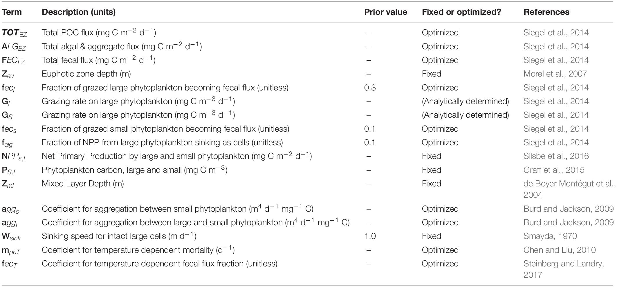
Table 1. Data product and parameter names, descriptions, and references used in the model configurations.

Baseline Food Web Model

The baseline model (S14; full details are available in Siegel et al., 2014) routes NPP through a two-size food-web model estimating the total POC flux (TOT_EZ, mg C m^–2 d^–1) at the base of the euphotic zone (Z_eu), which is determined as the sum of modeled fecal export (FEC_EZ) and sinking algal export (ALG_EZ), or

$${\mathbf{\text{TOT}}}_{\text{EZ}}=AL{G}_{EZ}+FE{C}_{EZ}.(1)$$

The fecal POC flux (FEC_EZ) is calculated by multiplying herbivory rate for each size class by fixed size-specific fecal flux fractions (fec_l, fec_s) that quantify the fraction of ingested carbon that becomes fecal flux (Table 1).

$$FE{C}_{EZ}=[(fe{c}_l\times G_l)+(fe{c}_s\times G_S)]\times Z_{eu}.(2)$$

Herbivory rates (G_l, G_S) are determined through mass balance using satellite observations of phytoplankton biomass (P, dP/dt) for each size class and net primary production (NPP, mg C m^–2 d^–1), an assumed mortality rate which includes death by viruses and cell lysis (collectively m_ph), modeled algal fluxes (ALG_sEZ, ALG_lEZ), and detrainment below the mixed layer ($\frac{P_s}{Z_{ml}}\frac{d{Z}_{ml}}{dt}H\left(\frac{d{Z}_{ml}}{dt}\right),$ Eqs 3a, b).

$$\mathit{\hspace{1em}\hspace{0.5em}}\frac{d{P}_s}{dt}=\frac{NP{P}_s}{Z_{eu}}-G_S-m_{phs}\times P_S-\frac{AL{G}_{sEZ}}{Z_{eu}}$$

$$\mathit{\hspace{1em}\hspace{0.25em}}-\frac{P_s}{Z_{ml}}\frac{d{Z}_{ml}}{dt}H\left(\frac{d{Z}_{ml}}{dt}\right).(3\mathrm{a})$$

$$\mathit{\hspace{1em}\hspace{0.5em}}\frac{d{P}_l}{dt}=\frac{NP{P}_l}{Z_{eu}}-G_l-m_{phl}\times P_l-\frac{AL{G}_{lEZ}}{Z_{eu}}$$

$$\mathit{\hspace{1em}\hspace{0.25em}}-\frac{P_l}{Z_{ml}}\frac{d{Z}_{ml}}{dt}H\left(\frac{d{Z}_{ml}}{dt}\right).(3\mathrm{b})$$

The last terms in Eqs 3a, b represent the reduction in phytoplankton carbon due to detrainment where Z_ml is the mixed layer and H(x) = 1 if x > 0 and 0 otherwise. When Z_ml deepens the grazing rate is decreased due to a more dilute prey environment, ultimately leading to decreased flux.

In S14, the algal POC flux (ALG_EZ) is modeled as a fixed fraction (f_alg = 0.1) of the NPP rate for large phytoplankton, or

$$AL{G}_{EZ}=f_{alg}\times NP{P}_l.(4\mathrm{a})$$

Overview of Model Configurations

Here, we alter the S14 model by evaluating the importance of four additional processes, namely aggregation of phytoplankton, the effects of both size and temperature on phytoplankton mortality, and the influence of temperature on zooplankton fecal flux, which adds seven new parameters to the model (W_sink, agg_l, agg_s, m_phs, m_phl, m_phT, fec_T) described below. There are mechanistic reasons to consider both temperature and size in formulations for carbon flux. Temperature affects animal metabolism and growth rate (Cael and Follows, 2016 and refs therein), and phytoplankton size is related to the number of trophic levels in the ecosystem, which affects grazing efficiency and the efficiency of the microbial loop (Michaels and Silver, 1988; Jackson and Burd, 1998).

The total algal flux (ALG_EZ) is modeled as the sum of the large (micro, 20–50 μm) and small (pico and nano, 0.5–20 μm) algal sinking fluxes:

$$AL{G}_{EZ}=AL{G}_{sEZ}+AL{G}_{lEZ}.(4\mathrm{b})$$

The small algal sinking flux (ALG_sEZ) is modeled as proportional to the square of the small phytoplankton carbon concentration. This follows the idea that aggregation scales with cell concentration (Burd and Jackson, 2009), or

$$AL{G}_{sEZ}=ag{g}_s\left(P_s^2\right).(4\mathrm{c})$$

The large algal sinking flux (ALG_lEZ) is modeled as the sum of directly-sinking large phytoplankton cells, plus an additional term to account for aggregation of large phytoplankton with both large and small phytoplankton, or

$$AL{G}_{lEZ}=W_{sink}\times P_l+ag{g}_l(P_l^2+P_l\times P_s).(4\mathrm{d})$$

Large phytoplankton are assumed to sink (W_sink, m d^–1) at a fixed rate of 1 m d^–1 [following observations of single cell sinking in Smayda (1970)]. We assume that the sinking flux of individual small phytoplankton is negligible. The two aggregation coefficients (agg_l and agg_s) are allowed to vary for the different size classes to account for differences in the surface area and sinking speed of large and small aggregates. Ideally every flux class would be modeled with a sinking speed but because our focus is on the export from the surface ocean, we choose to calculate general fluxes at the base of the euphotic layer and assume minimal transit distance for aggregate and fecal fluxes.

Temperature dependent mortality is modeled using a Q₁₀ of 2 with a reference temperature T₀ of 20 degrees C, following Chen and Liu (2010).

$$m_{phl,s}=m_{phT}\times Q_{10}^{\frac{\left(T-T_0\right)}{T_0}}.(5)$$

The value of the constant m_phT (d^–1) is not specified a priori, but is determined by a parameter optimization procedure (section “Model optimizations”). This formulation increases non-grazing mortality rates for warmer waters (e.g., the subtropics) compared to cooler waters in the high latitudes or along areas of upwelling. Under the temperature dependent mortality scheme, m_phl = m_phs using Eq. 5. We also test a configuration of the model in which m_ph is size-dependent but not temperature-dependent. In the size-dependent mortality model, m_phl and m_phs are different in order to account for the documented dependency of viral activity on phytoplankton size (e.g., Fuhrman, 1999).

Finally, fecal flux (FEC_EZ) is calculated by applying either size-specific or temperature-dependent fecal fractions to grazing rates. In S14, fec_s is 10% and fec_l is 30% to account for the fact that fewer trophic steps are involved in the transfer of larger phytoplankton to zooplankton, increasing the efficiency with which that food is processed. On the other hand, when prey is large compared to the predator, some biomass is thought to be lost through sloppy feeding (Lampert, 1978; Møller and Nielsen, 2001), which would reduce the POC available for export. Following optimization results in B18, we expect that fec_l will exceed fec_s. As in S14, total fecal flux is the sum of small and large fecal flux, or

$$FE{C}_{EZ}=[(fe{c}_l\times G_l)+(fe{c}_s\times G_S)]\times Z_{eu}.(6\mathrm{a})$$

Here we also model the influence of temperature on fecal flux via its impact on zooplankton metabolism. Roughly half of ingested carbon is respired by zooplankton, and there are even higher weight-specific respiration rates for zooplankton in the tropics and subtropics compared to colder polar regions (see Ikeda, 2014 and review by Steinberg and Landry, 2017). The documented effect of temperature on zooplankton respiration rates implies higher carbon loss in higher temperatures. To account for this carbon loss, we model the fecal flux fraction as an inverse function of sea surface temperature (T), or

$$fe{c}_{s,l}=fe{c}_T\times Q_{10}^{\frac{-\left(T-T_0\right)}{T_0}}.(6\mathrm{b})$$

The exponent in Eq. 6b is negative to account for decreasing fecal pellet production (i.e., increased respiration) as temperature increases. Under this formulation fec_s = fec_l and both fec_s and fec_l vary with sea surface temperature. T₀ = 20°C and a Q₁₀ value of 2 is used, following Ikeda (2014).

Specific Model Configuration Descriptions

From the components described above, we build and evaluate 6 different model configurations (in order of increasing complexity):

1. “One Size”: This model configuration has only one phytoplankton size class and three parameters:m_ph, fec, and agg. ALG_EZ is modeled as the square of total phytoplankton carbon concentration and an aggregation parameter: agg(P²). The herbivory calculation uses a single equation for phytoplankton mass balance, or

$$\frac{dP}{dt}=\frac{NPP}{Z_{eu}}-G-m_{ph}\times P-\frac{AL{G}_{sEZ}}{Z_{eu}}$$

$$-\frac{P}{Z_{ml}}\frac{d{Z}_{ml}}{dt}H\left(\frac{d{Z}_{ml}}{dt}\right).(7)$$

The expected value for the fecal flux fraction is 20%.

2. “S14”: This model is the original food-web model of Siegel et al. (2014), which uses four parameters: m_ph, fec_s, fec_l, and f_alg. The algal parameter (f_alg) is the fraction of NPP performed by large phytoplankton that becomes sinking POC. This model was optimized in B18 with the same POC flux data compilation that we use in the present study.

3. “Aggregation”: This model configuration is different from S14 because it calculates ALG_EZ for both large and small plankton using our aggregation formulation (see Eqs 4a–c) rather than assuming a fixed algal sinking fraction of NPP_L. In total, this model requires five parameters and assumes that m_phs = m_phl.

4. “Aggregation + Temperature Dependent Mortality”: This model configuration builds off the “Aggregation” model by introducing a temperature dependent mortality term (m_phT, see Eq. 5) in place of the size-dependent mortality terms m_phs and m_phl, totaling five parameters.

5. “Aggregation + Temperature Dependent Fecal Flux”: This model configuration builds off the “Aggregation” model by prescribing a temperature dependent fecal flux (fec_T, see Eq. 6b) rather than size dependent fecal terms (fec_s, fec_l), totaling five parameters.

6. “Aggregation + Size Mortality”: This model configuration builds off “Aggregation” and uses six parameters in total: the two ALG_EZ free parameters based on size, the two FEC_EZ parameters based on size, as well as m_phs and m_phl.

Model Optimizations

We optimize the free parameters (agg_s, agg_l, m_phs, m_phl, m_phT, fec_s, fec_l, fec_T, and f_alg) of the 6 models listed above with the goals of finding parameter values that minimize the model/data misfit while retaining reasonable fidelity to prior expectations of parameter values. The procedure follows that used by B18 and will be briefly described here. The fitting metric is the log posterior function, which combines the model-data misfit for POC flux (the log likelihood) with penalties for parameter deviations from what is expected based on previous understanding (the log prior).

The log posterior is the sum of the log likelihood and the log prior:

$$\log \mathrm{posterior}=\log \text{likelihood}+\log \mathrm{prior}.(8)$$

The model-data mismatch is minimized when the log likelihood is maximized:

$$\log \text{likelihood}=-\frac{{\sum }_{i=1}^N{\left[\text{log}(POCflu{x}_{mod}/POCflu{x}_{obs})\right]}^2}{N}.(9)$$

Modeled and observed POC flux (POCflux_mod, POCflux_obs, respectively) are log transformed because the observed POC fluxes follow a lognormal distribution. N = 14 is the total number of POC flux observations in the dataset of B18, which was constructed by averaging 165 independent POC flux observations onto a regular 1-degree grid with monthly resolution (see B18 for full details). The log prior is formulated as in B18 but is normalized by the total number of parameters in each model (n_p) so that any one model is not disproportionately penalized for additional parameters. The log prior quantifies the departure of an optimized parameter from its expected value,

$$\log \mathrm{prior}=-\frac{{\sum }_{k=1}^{k=n_p}{\left(\text{log}(paramete{r}_n)-\text{log}(expecte{d}_n)\right)}^4}{n_p}.(10)$$

With this formulation, the magnitude of the log posterior is dominated by the log-likelihood, rather than the log-prior. The parameters are log transformed as in B18 to force parameter values to be positive, and to apply large penalties to large deviations from the expected value.

All model configurations are optimized using a “Climatological Dataset” of POC export (section “Input data”) using slice sampling (a type of Markov chain Monte Carlo algorithm) as described in B18. Briefly, for each model configuration we draw random initial parameter values (x_0,k) equal to the number of parameters (k) in each model experiment from a uniform distribution within (0,1]. The posterior function is calculated, and the parameter values are iteratively updated using the slice sampling algorithm (Neal, 2003). This is repeated until we have a “chain” of 2000 samples for each parameter (Neal, 2003). We run 4 chains independently and sampling is stopped once the four chains converge to the same probability density function [quantified by a “Potential Scale Reduction Factor” near 1 (Brooks and Gelman, 1998)]. The first 50% of the samples are discarded as part of the “burn-in” phase and the remaining parameter values are included in the sample. The reported parameter uncertainties represent half the interquartile range of the sampled parameters. Reported POC flux uncertainties are half the interquartile range of POC fluxes generated using all of the sampled parameters. The model results are also scored using the Pearson correlation coefficient (r) and the Root Mean Square Difference (RMSD) to give a more comprehensive understanding of the model performance.

POC Export Parameter Sensitivities

To understand how each parameter affects the modeled POC export, we calculate the sensitivity of POC export to each parameter in each model configuration (section “Overview of model configurations”). The POC export sensitivity to parameter k is calculated using a centered finite difference perturbation (DP) to parameter k while all other parameters are fixed. We choose DP to be half the interquartile range for the parameter values generated from slice sampling and we calculate the centered difference as ^1/2(POC_{p + DP}–POC_p) + ^1/2(POC_p–POC_p–DP). Here POC_p is the flux for a particular parameter set (p) and POC_{p + DP} is the flux after parameters are altered by adding (p + DP) or subtracting (p–DP) a difference perturbation (DP).

To quantify the sensitivity of global POC export to parameter choice, we draw 1000 optimized parameter samples for a given model so that the covariances among the optimized parameters are considered. We then compute the modeled POC export using the 1000 different parameter values and report half the interquartile range as the POC export uncertainty (as shown in Figure 2D).

Input Data

The models take as input monthly mean observations from the Sea-Viewing Wide-Field-of-View Sensor (SeaWiFS) satellite ocean color mission from September 1997–December 2008, as is done in S14 and B18 (Supplementary Figure 1). In this study we use the Carbon, Absorption and Fluorescence Euphotic-resolving (CAFE) NPP satellite data product (Silsbe et al., 2016) because it showed the best performance across all of the datasets analyzed in B18 and because it showed best performance with in situ NPP measurements compared to other NPP models. The choice of NPP product will affect parameter values to an extent, but the variations in parameter values introduced by different NPP products are small compared to parameter uncertainties (see Figure 4 in B18).

In addition to NPP (mg C m^–2 d^–1), the model also takes as input the phytoplankton size distribution (Kostadinov et al., 2010), the euphotic zone depth [m, derived from satellite chl concentrations using equations in Morel et al. (2007)], phytoplankton carbon [P, mg C m^–3, derived from satellite derived particulate backscatter (443 nm, m^–1) using the relationship in Graff et al., 2015], and mixed layer depth (m, provided by the MLD_DT02 climatology, de Boyer Montégut et al., 2004). Sea surface temperatures to calculate temperature-dependent mortality and fecal flux terms are taken from the annual average World Ocean Atlas 2013 maps (Locarnini et al., 2010).

We organize the data as follows: all data inputs are gridded onto a 1-degree latitude/longitude grid and averaged for each climatological month (Supplementary Figure 1). As in S14, we require a minimum of 8 months a year of observations, which effectively excludes regions poleward of ∼65^o latitude from analysis.

Model Test Dataset

For POC flux observations, we use the B18 “Climatological Dataset” of POC export. The B18 “Climatological Data” includes 165 total observations of POC flux at the Z_eu depth from the ²³⁴Th technique at 14 different sites, with an average flux of 69 mg C m² d^–1. The dataset is spatially biased toward the Northern Hemisphere and does not include fluxes in the high latitudes or the Indian Ocean (Supplementary Figure 2), but is used for optimization because each grid cell contains multiple observations of POC export, such that the average POC export within each grid cell is a 1-degree, monthly average. In this way, the data and model outputs are evaluated at the same spatiotemporal resolution and depth.

Results

Estimated Parameter Values for All Models

Optimized parameter values for the suite of six model configurations are shown in Figure 1. We expect that some parameter values will vary from the B18 values because when new parameters are added, additional degrees of freedom are added as well. This is evident when comparing “S14” to the more complex model configurations because these model configurations are identically formulated apart from their aggregation, fecal flux, or mortality parameterizations. The optimized parameter values for the “S14” and “Aggregation” models are very similar, but both of these are substantially different from the “One Size” model (compare the first through third bars for m_phs, m_phl, fec_s, fec_l). When differential mortality based on size is added to the “Aggregation” model (i.e., the “Aggregation + Size Mortality” model) the mortality rate for large phytoplankton nearly doubles.

FIGURE 1

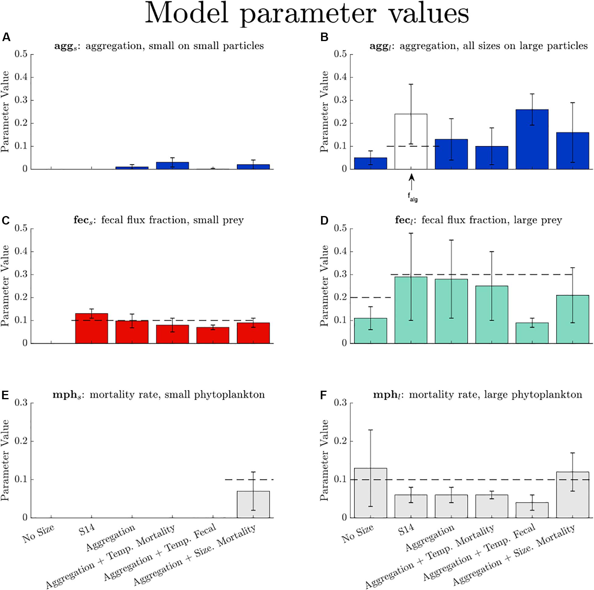
Figure 1. Parameter values and their uncertainties for the five model configurations and the base model, S14. Expected parameter values are given by a dashed line when appropriate (see Table 1 for references). Error bars represent half the interquartile range retrieve set of optimized parameter values: (A) agg_s, (B), agg_l, (C) fec_s, (D) fec_l, (E) mph_s, and (F) mph_l. The f_alg term is from the S14 model and is a different parameterization than either agg_s or agg_l. The f_alg term represents the fraction of NPP that becomes sinking algal flux. For models involving a temperature dependency (“Aggregation + Temp. Mortality” and “Aggregation + Temp. Fecal,” the parameter value represents the coefficient in the Q10 formulae (see Eqs 5, 6b). For models when size is not included for a parameter we show the parameter value in the large fraction (e.g., for “One Size,” the overall fecal flux fraction is shown in the fec_l panel.).

There are slight departures in the parameter values from their expected values (if applicable), given by dashed lines in Figure 1. Most model configurations predict a reduced rate of small and large phytoplankton mortality from prior values and a slightly reduced fecal flux fraction for large prey. While there were no expected values for the two aggregation terms, there are variations in both the magnitude and the range of agg_s and agg_l, and agg_s is always less than agg_l. Thus, the aggregation model configurations predict that more large cells will sink as aggregates compared to small cells, given equivalent biomass in both phytoplankton size classes.

Model Skill, Sensitivities, and Global Statistics

Results from the model optimizations are shown in Figure 2. Model skill is evaluated on the basis of the log likelihood, the correlation coefficient, and the RMSD. The log likelihood increases with increasing degrees of freedom, as expected. However, the increase in model degrees of freedom does not correspond to improvement in other performance metrics. The correlation coefficient is reduced in the case of the “Aggregation + Size Mortality” compared to the “Aggregation” model, and the RMSDs are higher for the “Aggregation + Size Mortality” and “Aggregation + Temperature Mortality” model configurations. The “One Size” model performs the worst: it has the lowest correlation coefficient, the highest RMSD, and the largest log posterior absolute value. Because of the poor performance for the “One Size” model, we focus the bulk of our results and discussion on the other models. We include the “One Size” model in the figures to highlight the importance of resolving different phytoplankton size classes for predicting POC export. Apart from the “One Size” model, there is not a substantial difference in performance across the model configurations, as measured by the model-data misfit for POC export. There is also little change in the globally integrated POC export for all the model configurations, which ranges from 6.1 ± 1.3 Pg C year^–1 in the “One Size” model to 7.2 ± 0.5 Pg C year^–1 in the “Aggregation” model. All models predict similar global POC export values because the parameters of all models are optimized with the same POC flux dataset.

FIGURE 2

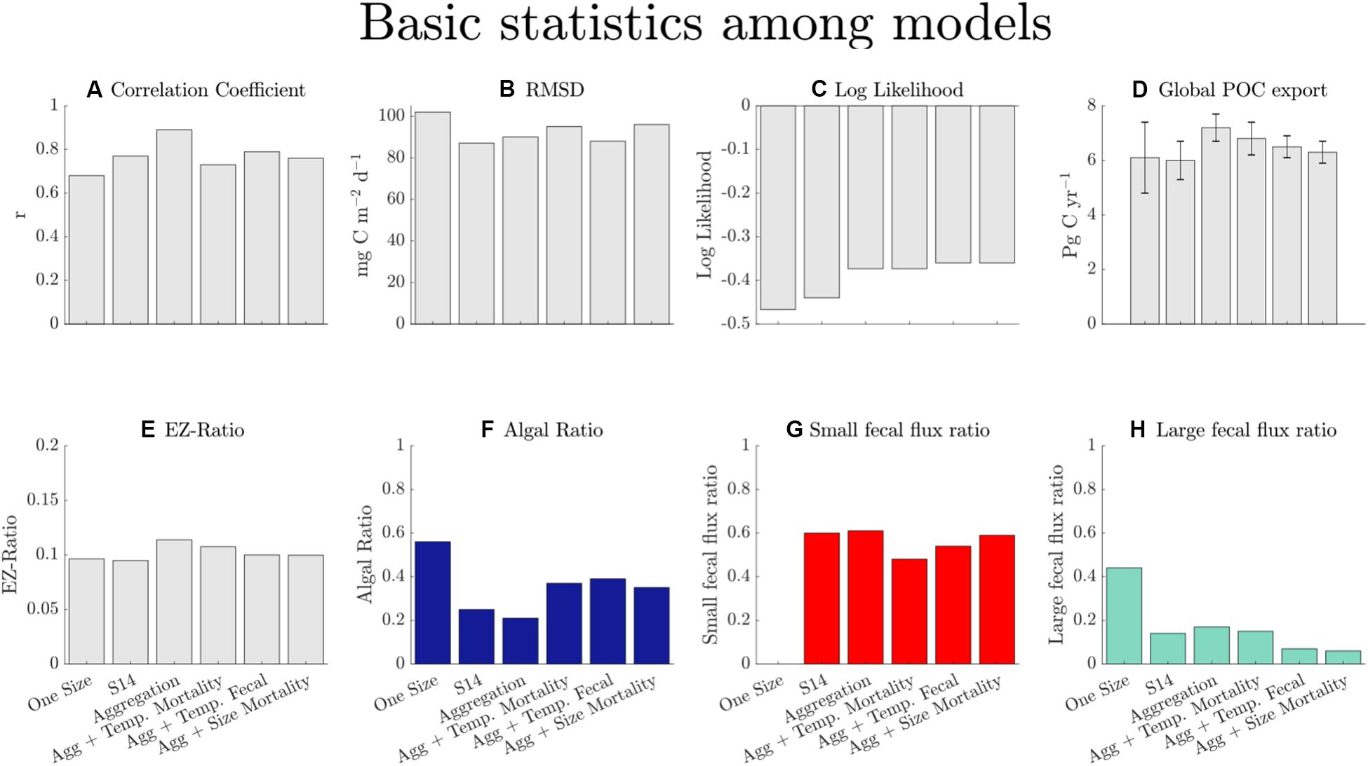
Figure 2. Basic statistics for the six models in order of increasing number of parameters (from 3 in the case of “One Size,” to 6 in the case of “Aggregation + Size Mortality”). The correlation coefficient (A) is given by Pearson’s r, RMSD (B) is the root mean squared difference, and the log likelihood (C) is described in equation 9. The error bars on integrated model flux (D) values represent half the interquartile range from POC flux simulations. The EZ-ratio (E) is the flux at the base of the euphotic zone divided by NPP. The algal ratio (F) is the fraction of total export contributed by direct algal sinking and aggregation. The small fecal (G) and large fecal (H) flux ratios are the fraction of fecal flux to total export for small and large zooplankton, respectively. Note that the y axis limits vary for different parameters.

Although the magnitude of POC export is similar across all models (Figures 2D, 3A), the fractional contribution of the different POC export mechanisms to the total export varies substantially (Figures 2F,H, 3B,C). Discarding the unrealistic “One Size” model, the algal ratio (the fraction of total POC export due to sinking phytoplankton cells and aggregates) varies between 21% in the “Aggregation” model and 39% in the “Aggregation + Temperature Mortality” model (Figure 3C). The fraction of small fecal flux to total POC flux is the most consistent across model configuration, varying from 48% in the “Aggregation + Temperature Mortality” model to 61% in the “Aggregation” model (Figures 3B,C). The fraction of large fecal flux to total POC flux varies from 6% in the “Aggregation + Size Mortality” model to 17% in the “Aggregation” model. In all model configurations, the small fecal flux is the dominant pathway for total POC flux, especially in the gyres where it contributes to >75% of the total POC export (Figure 3C). The globally-integrated rate of POC export via small fecal flux ranges from 3.2 Pg C year^–1 in the “Aggregation + Temp Mortality” model to 4.4 Pg C year^–1 in the “Aggregation” model. The implications of this are discussed in section “Discussion.”

FIGURE 3

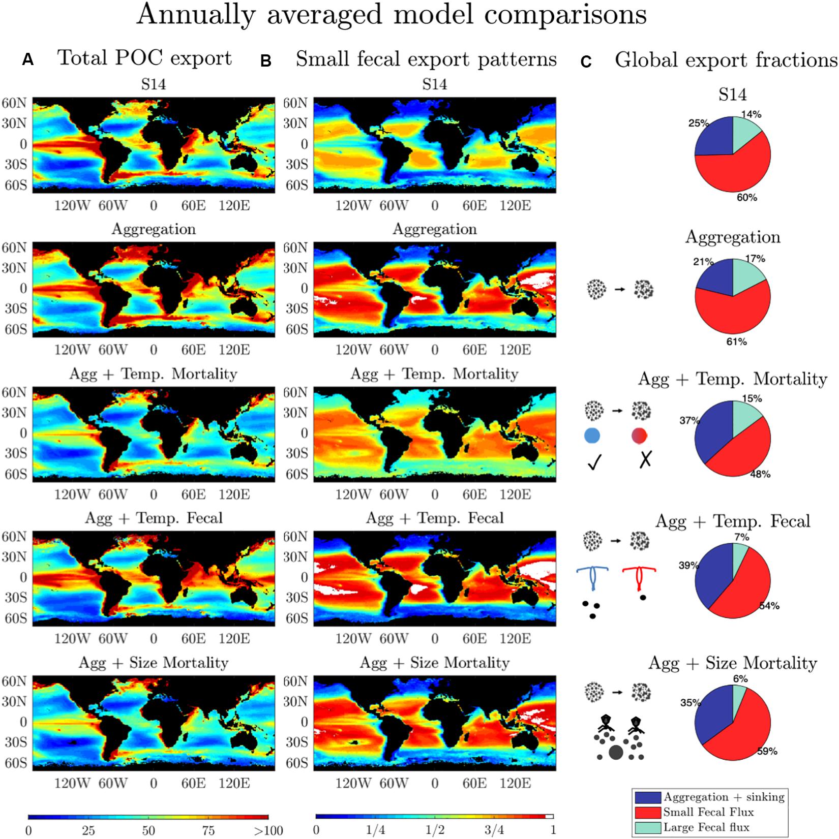
Figure 3. (A) Annually averaged total POC export (mg C m^–2 d^–1). (B) Annually averaged contribution of small fecal flux to total POC export. (C) The fraction of annual average small fecal flux, large fecal flux, and aggregation and sinking flux to total flux for the 5 five models that incorporate phytoplankton size into their formulations.

Spatial and Temporal Variability of POC Export Pathways

The model results can be used to assess the magnitude, spatial variability, and timing of particular mechanisms to the total POC export. Regions with different magnitudes of total POC export (i.e., oligotrophic vs. high latitude regions) differ in both the magnitude and timing of the various POC export pathways throughout the annual cycle (Figure 4). The peak timing of aggregation and sinking flux occurs in June for the North Atlantic, August for Station P in the North Pacific, and there is no substantial change in aggregation and sinking flux for Station Aloha. Throughout the year in the North Atlantic, the large fecal flux exceeds or matches that of small fecal flux in most models; however, in the North Pacific the small fecal flux exceeds the large fecal flux in most models throughout most of the year, and small and large fecal fluxes are negatively correlated (R ∼ -0.7 for all models). To first order, the seasonal changes in flux are driven by seasonal changes in NPP as well as the particle size distribution. In general, the seasonal variability of the various export pathways is similar across all models for any particular site, but the magnitudes of different export pathways vary among models (Figure 4).

FIGURE 4

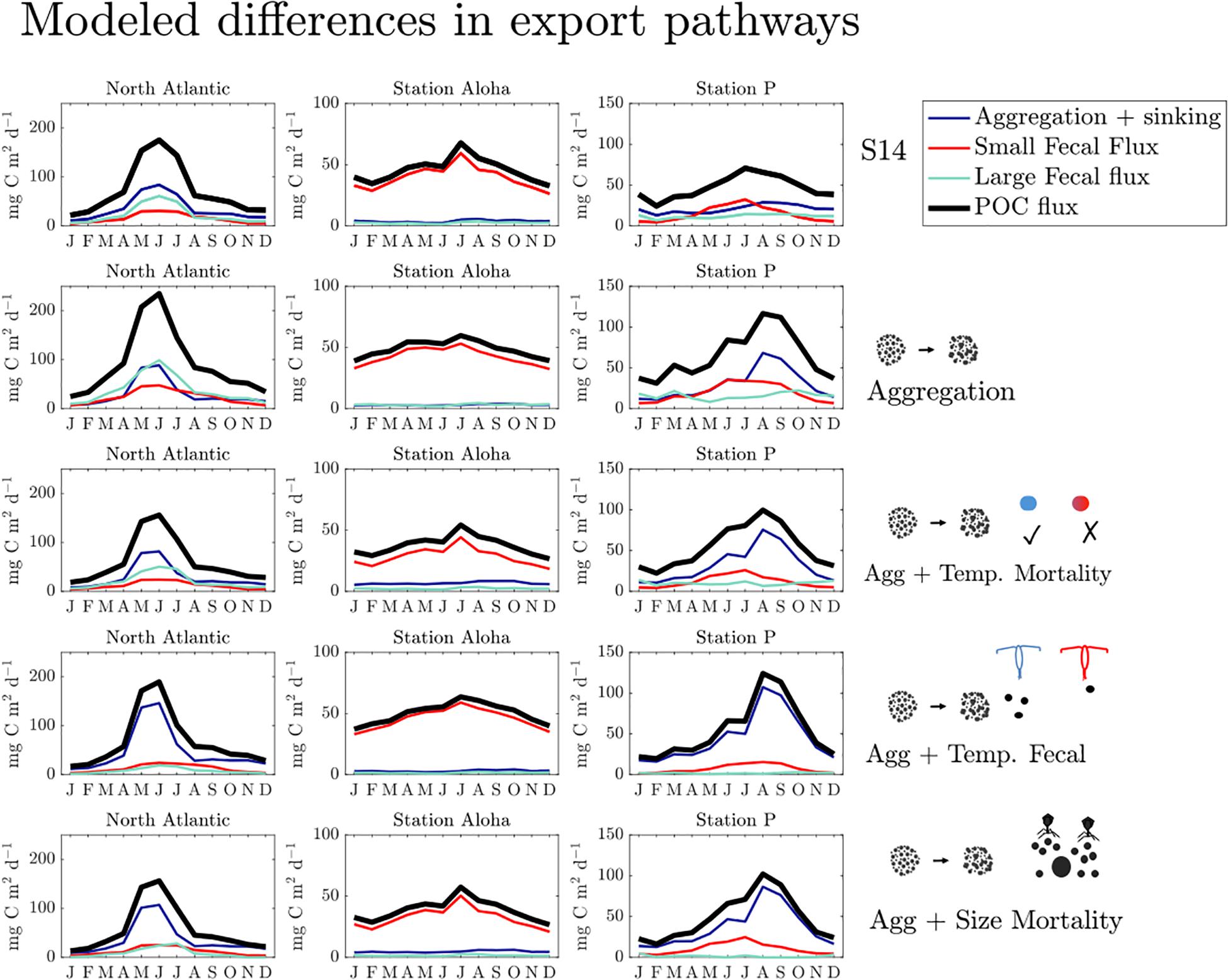
Figure 4. Seasonal variability of POC export for all models with two size classes for the North Atlantic (47N, 20W), Station Aloha (22N, 158W), and Station P (50N, 145W). Note the different y-axis scales for each location. The POC export by three different pathways (aggregation and sinking, small fecal flux, large fecal flux) is shown, along with total POC export (in black). Icons next to the graphs are qualitative model representations, as used in Figure 3.

The dominant POC export pathway on global scales is the small fecal flux pathway, followed by the aggregation and large fecal export pathways (Figure 3). Across all models, there are consistent qualitative patterns in the sensitivities of POC export to any one particular parameter, although the magnitude of these sensitivities varies from model to model (Figure 5 and Supplementary Figures 3, 4). POC export in all models is most sensitive to the fec_s parameter, as illustrated for the “Aggregation” model in Figure 5. After the fec_s parameter, the greatest sensitivity is to fec_l, followed by m_phl,s, agg_l, and agg_s (Figure 5, on the basis of the median sensitivity). The magnitude of sensitivity can be compared to annual mean POC flux, which is 65 mg C m^–2 d^–1 for the “Aggregation” model. A sensitivity value of 20 mg C m^–2 d^–1 corresponds to 30% of annually averaged flux. Although the global sensitivities average between -3 and 8 mg POC m^–2 d^–1, they can exceed 20 mg POC m^–2 d^–1 on annually averaged regional scales, especially for fec_s and fec_l. The models are especially sensitive to agg_l, f_alg, and fec_l along coasts and areas of upwelling where there is a higher fraction of large phytoplankton. The reverse is true for the fec_s term, where increasing fec_s especially increases POC export in the tropics. For all models, increasing agg_l, f_alg, and fec_s,l yields higher POC export, and increasing m_phs, m_phl, and m_phT yields lower POC export. These parameter sensitivities highlight regions where additional data will be especially useful. For example, the Equatorial Pacific, the Southern Atlantic Ocean, and the Northern Indian Ocean have high sensitivity to the fec_s, and/or fec_l terms. Field observations of fecal flux fractions in these regions may significantly improve these models.

FIGURE 5

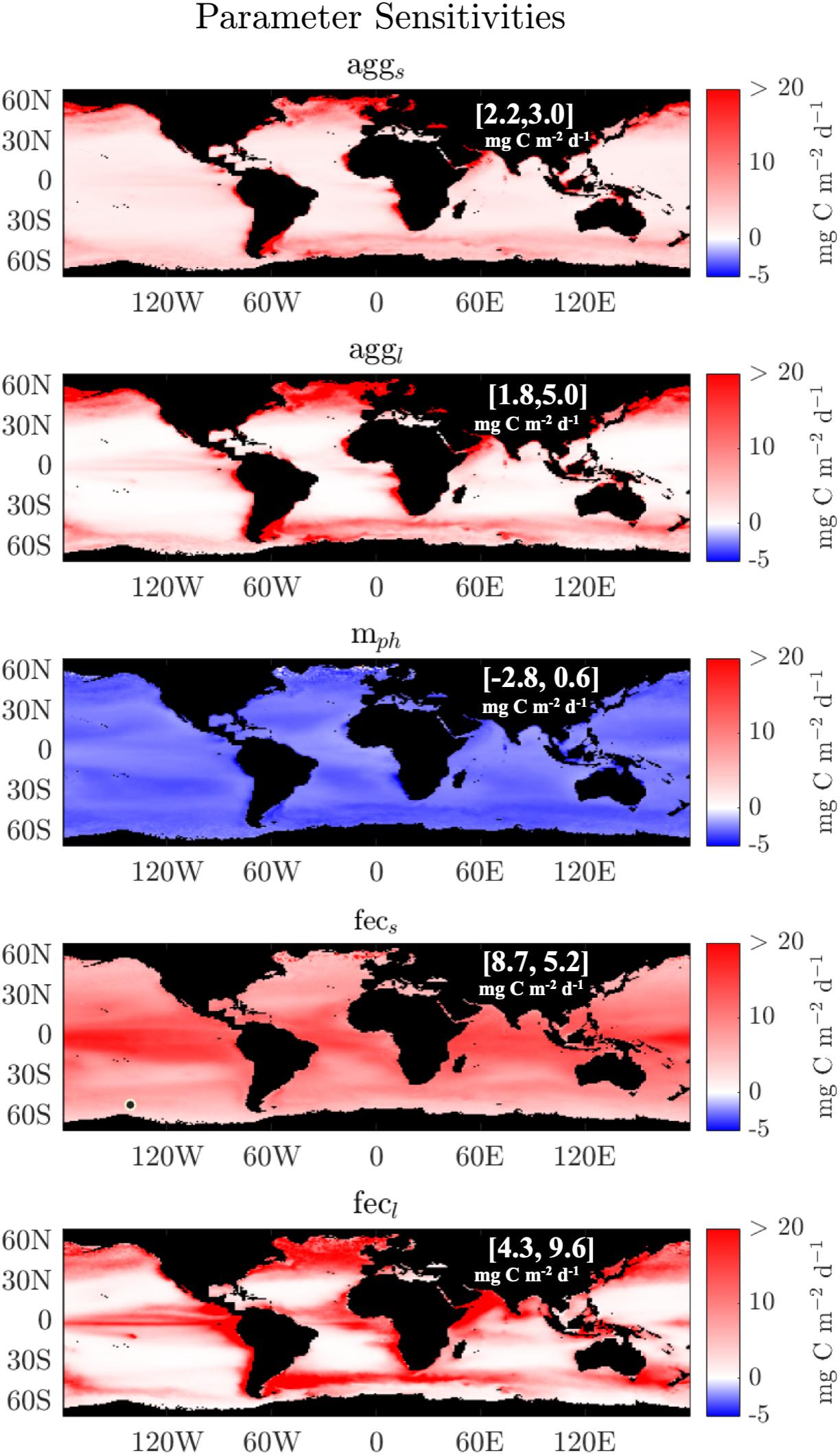
Figure 5. Global maps showing sensitivity of POC export (in units (mg C m^–2 d^–1) to parameters in the “Aggregation” model. The values are given by a centered difference, or ^1/2(POC_{p + DP}–POC_p)+ ^1/2(POC_p–POC_p–DP), where DP is half the interquartile range for a given parameter from the set of parameters retrieved by the slice sampling algorithm. The median sensitivity (left) and its interquartile range (right) are bracketed.

Discussion

Importance of Resolving Ecosystem Size Structure

In this study we found that resolving two size classes of phytoplankton substantially improved the ability of our model to match observed POC export fluxes. These results are important for guiding the development of future Earth system modeling of the biological pump. The “One Size” model performed poorly against observations of POC export (on the basis of RMSDs and correlation coefficient) and its optimized parameter values were unrealistic. The predicted fraction of algal sinking to total flux is 60% for the “One Size” model, which is an unrealistically high fraction on annual global scales (Burd and Jackson, 2009). The algal fraction in the other model configurations is between 20–40%, which is more reasonable. The “One Size” model is also more sensitive to parameter changes compared with the other model configurations, and has the largest uncertainty of integrated POC export of all models (Figure 2). These findings, together with the poor model-observations misfits for the “One Size” model, underscore the importance of resolving at least two phytoplankton size classes in a food web POC export model.

In contrast, adding explicit mechanisms beyond those already implemented in the “S14” model results in only incremental improvement (compare performance metrics in Figure 2). The taper in performance with added processes beyond those related to phytoplankton size demonstrates limitations in our model, since increasing model complexity only results in marginal improvements to model performance. The slight difference in performance among the models herein obscures our ability to judge any given model configuration solely on the basis of its ability to match observations of POC export. The models do, however, vary in the predicted mechanisms of POC export (see Figures 4, 5). Measurements that quantify both the magnitude and mechanism of POC export would help to better distinguish between the models presented here, and help to improve mechanistic POC export models (see section “Conclusion”).

Importance of Small Phytoplankton and Zooplankton to Global Export Fluxes

In this study we optimized parametrizations for mechanistic processes contributing to POC flux. We found that the dominant passive POC export pathway on global scales is from small zooplankton fecal flux, and that the annually averaged model sensitivity to fec_s term is ∼9 mg C m^–2 d^–1 (∼15% of annual POC export) in the “Aggregation” model (Figure 5). For the aggregate flux pathway, large aggregates are more important globally than smaller aggregates (compare Figures 6B,C). However, small phytoplankton aggregates provide a steady background flux of ∼ 2 mg POC m^–2 d^–1 globally (Figure 6C). Our study finds enhanced aggregation by small cells in the oligotrophic gyres compared to other areas, which supports work (Chow et al., 2015 and refs therein) demonstrating that small cells can become sticky and aggregate when under nutrient stress. In the subtropical gyres where small phytoplankton dominate, small aggregates constitute >75% of the total aggregate flux (Figure 6D), although the bulk of the export in these regions is from small zooplankton fecal pellets. Large aggregates dominate in high-productivity regions such as the coastal, upwelling, and seasonal bloom regions. Direct sinking of intact phytoplankton cells accounts for a much smaller fraction of total POC export than either large or small aggregates (Figure 6A).

FIGURE 6

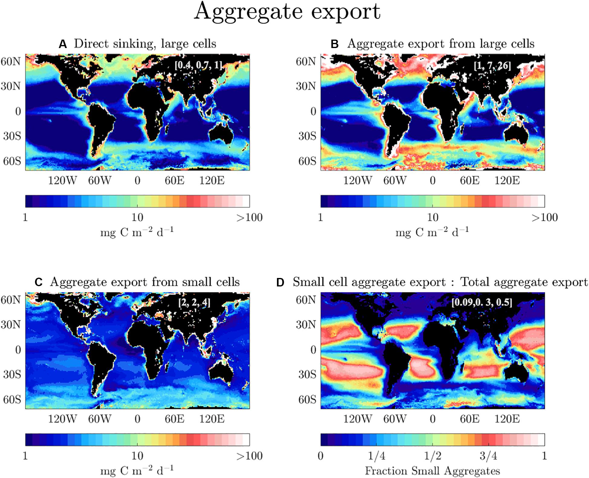
Figure 6. Annually averaged POC export in the “Aggregation” model by direct sinking of (A) large phytoplankton cells, (B) large phytoplankton aggregates, and (C) small phytoplankton aggregates. The bracketed values shown in each map are the 25th, 50th, and 75th quantiles for flux (mg C m^–2 d^–1), respectively. (D) The ratio of small phytoplankton aggregates to the total aggregate export. The bracketed numbers represent the 25th, 50th, and 75th quantiles for this ratio.

POC export derived from small phytoplankton (via small algal aggregates or fecal pellets produced by zooplankton that feed on small phytoplankton) dominates global POC flux in our models. This is primarily because small phytoplankton are much more common than large phytoplankton in most of the ocean, but we should also note that our model configurations predict POC export based on climatological conditions and will miss transient blooms that are often characterized by high POC export derived from large phytoplankton. Several recent studies have also examined the contribution of sinking small phytoplankton export to total POC flux. For example, Durkin et al. (2015) found that small cell export via small sinking particles contributed up to 67% of total POC flux, and Lomas and Moran (2011) found that pico- and nano- aggregates alone contributed up to 40% of total POC flux, both in the Sargasso Sea. Stukel et al. (2013) found that while Synechococcus contributed roughly a quarter of NPP, it only accounted for ∼6% of total POC flux in the Costa Rica upwelling dome, where the bulk of the flux came from mesozooplankton fecal pellets. Baker et al. (2017) found that POC concentrations of slowly sinking particles were up to 75 times greater than fast sinking particles in the deep Atlantic, and that slow sinking export fluxes generally exceeded fast sinking export fluxes. These studies represent snapshots in time compared to average values that we report herein. Still, more work is needed to comprehensively assess the role of small phytoplankton to total export on global scales (Richardson, 2019).

In this study, when the small fecal flux is larger than the large fecal flux, it is typically >50% of the total flux. When the large fecal flux is larger than the small fecal flux, it is usually not the dominant flux pathway, contributing between 20% and 40% of total flux on average (depending on the model configuration used). Ultimately our study findings are similar to what is found in previous work: even when large zooplankton are present, small phytoplankton (via aggregation or small sinking fecal pellets) can contribute a large portion of total flux (Richardson, 2019 and refs therein).

For decades, large particles and aggregates have been thought to contribute the majority of carbon flux, making it difficult to reconcile the relatively low proportion (∼1%) of primary production reaching a climatically-relevant depth horizon (∼1000 m). Our finding that small particles are the bulk of sinking carbon flux exiting the euphotic zone may help close the gap between observations at depth and at the surface, where many studies have focused on the contribution of large cells to flux.

Modeled Herbivory Rates and Comparison With Grazing Experiments

As noted above (Figure 3), the total POC export is similar across all the different model configurations compared here. This makes it difficult to constrain or distinguish between these different mechanistic model configurations on the basis of POC export alone. However, the model configurations can be evaluated with observations other than POC export. For example, the models also predict zooplankton herbivory rates, which have been measured in experiments and for which global syntheses are available (Calbet and Landry, 2004; Schmoker et al., 2013). Figure 7 shows model-predicted herbivory rates on small and large phytoplankton, which is analogous to grazing by microzooplankton and mesozooplankton in our two-size food web model. Previous work estimated global mean values for the fraction of NPP consumed by microzooplankton to be ∼60–70% (Calbet and Landry, 2004; Schmoker et al., 2013; Sherman et al., 2016). We compare our model configuration results to the compilation of Sherman et al. (2016), which provides phytoplankton growth and microzooplankton grazing rates. For consistency with our model configurations, we calculate the ratio of phytoplankton growth to microzooplankton grazing and eliminate instances in this ratio where the grazing fraction exceeds one or is negative. The mean fraction of herbivory on small phytoplankton relative to total NPP in our models is 53% for “S14,” 69% for “Aggregation,” 50% for “Aggregation + Temperature Dependent Mortality,” 74% for “Aggregation + Temperature Dependent Fecal Flux,” and 46% for “Aggregation + Size Mortality” (see Figure 7, and note the median values are displayed). This fraction is largest in the “Aggregation + Temperature Dependent Fecal Flux” model because its agg_s parameter is smaller than agg_s for all other model configurations, so nearly all of the small phytoplankton NPP is available to be consumed because it does not become sinking aggregates. The “Aggregation” model performs closest to what is expected from microzooplankton grazing experimental results although it overestimates the proportion of grazing. All model configurations exhibit a smaller interquartile range than in the Sherman et al., 2016 grazing compilation. This difference is likely because the model predictions are averaged over larger spatial scales and longer time scales than the experiments.

FIGURE 7

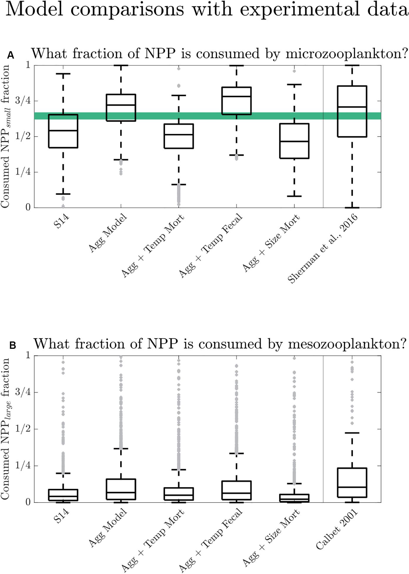
Figure 7. (A) Box and whisker plots of the annually averaged grazing rate of small zooplankton (Grz_s) divided by total NPP for the five models that have two phytoplankton size classes. The horizontal green shading indicates the range of global averages from previous studies (Schmoker et al., 2013 with a value of 0.62; Calbet and Landry, 2004 with a value of 0.67) for comparison. We include microzooplankton data from a recent compilation by Sherman et al., 2016. (B) Box and whisker plots of the annually averaged grazing rate of large zooplankton (Grz_l) divided by total NPP for the five models that have two phytoplankton size classes, and for data digitized from Calbet (2001; their Figure 1A).

Predicted grazing rates on large phytoplankton from the present model configurations can be compared to experimental mesozooplankton grazing data (Calbet, 2001, Figure 7B, digitized via < https://automeris.io/WebPlotDigitizer/ > with uncertainty < 5%). The experimental grazing rates were determined by gut pigment content and clearance rates from incubations. No direct matchups are available so we evaluate them on the basis of their frequency distribution functions, illustrated with box and whiskers plots. For consistency with our model configurations, we eliminate the few instances in the experimental data set where the grazing fraction exceeds one. The laboratory experiments show a higher fraction of production grazed by mesozooplankton than any of the models: the median of the Calbet (2001) data is 10%, compared to the median of the “S14” model (4%), the “Aggregation” model (7%), the “Aggregation + Temperature Dependent Mortality” model (5%), the “Aggregation + Temperature Dependent Fecal Flux” model (6%), and the “Aggregation + Size Mortality” model (2%). As is true for the small zooplankton grazing rates, the “Aggregation” model comes closest to the experimental data. In the case of both small and large grazing data there is insufficient data available to address the degree to which the models represent average grazing conditions in nature. Ideally there would be grazing data representing a “monthly average” for locations on a 1 × 1 degree grid.

Conclusion

In this study we extended the S14 satellite-based food web and carbon export model to include additional processes that are thought to influence POC export. We do not endorse any one model configuration presented herein as the “best,” because all model configurations were able to provide similar fits to observed POC export fluxes, after optimization of uncertain parameters. This highlights the limitations of using POC flux observations to guide the development of mechanistic models of POC export, and suggests that additional data are needed to choose the best configuration for these models. Aside from this limitation, several important points emerge from our analysis:

1. Including two phytoplankton size classes (rather than one) significantly improved model performance. In contrast, adding a mechanistic representation of aggregation, or including temperature-dependent grazing or mortality, did little to improve model performance.

2. Across all model configurations on global scales, the sinking fecal pellets of small zooplankton are the largest contributor to globally-integrated POC export.

3. All of the model configurations predict that the North Pacific experiences peak export in August, whereas the North Atlantic experiences peak export in June. All the different model configurations also predict that phytoplankton aggregates are the dominant carbon export pathway in these regions. The magnitude of the small zooplankton fecal flux is similar for both regions, but the relative contribution of this pathway is larger in the North Pacific than in the North Atlantic.

What data are needed to improve mechanistic models of carbon export such as the ones presented here? Ideally, total POC export would be measured simultaneously with measurements of the fraction of fecal pellets and phytoplankton aggregates contributing to export, in order to provide better constraints on the contribution of these flux pathways (and others) to POC export on regional to global scales. Also, ecosystem measurements such as rates of zooplankton grazing and phytoplankton aggregation would be useful for model evaluation and selection (e.g., Sherman et al., 2016; Le Moigne, 2019), especially if there are sufficient measurements available to average over a 1-degree monthly grid. In order to properly characterize sinking speed and remineralization rates for these flux pathways as they transit through the surface ocean into the deep, it is necessary to resolve particle composition. The EXPORTS program (United States; Siegel et al., 2016) and similar field campaigns [including FLUXES (Spain), COMICS (United Kingdom), GOCART (United Kingdom), CUSTARD (United Kingdom), Ocean Twilight Zone (United States), PICCOLO (United Kingdom), and more] will provide a diversity of measurements that may enable these comparisons on a regional scales, especially via data sharing efforts such as JETZON¹. Although not explicitly addressed in this paper, the ongoing development of mechanistic models driven by satellite products will benefit from data enabling characterization of surface phytoplankton communities beyond bulk assessments of phytoplankton carbon (see Kramer and Siegel, 2019) because different phytoplankton types are likely to have different potential for export via the aggregate and fecal flux pathways as modeled here. Advancements in satellite algorithms (particularly for b_bp because it quantifies NPP, phytoplankton carbon, and phytoplankton size, e.g., Loisel et al., 2018; Bisson et al., 2019) will also improve model fidelity by providing more accurate input data with reduced uncertainty.

Data Availability Statement

The datasets analyzed for this study are publicly provided by the NASA Ocean Biology Progressing Group (https://oceancolor.gsfc.nasa.gov). The carbon flux data are available at https://doi.org/10.1029/2018GB005934.

Author Contributions

KB, DS, and TD conceived this study. KB performed the analyses and made the figures. KB led the writing with input from DS and TD. All authors contributed to the article and approved the submitted version.

Funding

Support for this work came from the National Aeronautics and Space Administration (NASA) to DS as part of the EXport Processes in the Ocean from RemoTe Sensing (EXPORTS, grants 80NSSC17K0692 and NNX16AR49G). TD acknowledges support from NASA grant NNXAI22G.

Conflict of Interest

The authors declare that the research was conducted in the absence of any commercial or financial relationships that could be construed as a potential conflict of interest.

Acknowledgments

Thank you to Sasha Kramer, Craig Carlson, and Mark Brzezinski for helpful discussions, and to the OCB program for travel funding to the BIARITTZ conference. We are grateful for the reviewers comments that enhanced this work.

Supplementary Material

The Supplementary Material for this article can be found online at: https://www.frontiersin.org/articles/10.3389/fmars.2020.00505/full#supplementary-material

FIGURE S1 | Annual climatologies for selected satellite data inputs into the model. Phytoplankton carbon is in mg m^–3 and approximated using particulate backscatter at 443 nm (m^–1) using the relationship in Graff et al., 2015.

FIGURE S2 | The distribution of the data values is shown along with the data locations for the 14 sites used in this study.

FIGURE S3 | Global annually averaged maps showing model sensitivity in POC flux to changes in parameter value (DP, given by half the interquartile range) from the optimized parameter value (p). The values are given by a centered difference, or ^1/2(POC_{p + DP}–POC_p) + ^1/2(POC_p–POC_p–DP). In the case of “Aggregation + Temp Mortality,” and “Aggregation + Temp Fecal” the m_ph values reported are for the coefficients in the Q10 formulae. The median centered difference POC flux (left) and its interquartile range (right) are bracketed. The red text is to emphasize that the S14 values are for f_alg and not agg_s or agg_l.

FIGURE S4 | Global annually averaged maps showing model sensitivity in POC flux to changes in parameter value (DP, given by half the interquartile range) from the optimized parameter value (p). The values are given by a centered difference, or ^1/2(POC_{p + DP}–POC_p) + ^1/2(POC_p–POC_p–DP). In the case of “Aggregation + Temp Mortality,” and “Aggregation + Temp Fecal” the m_ph values reported are for the coefficients in the Q10 formulae. The median centered difference POC flux (left) and its interquartile range (right) are bracketed. The values and maps for m_phs and m_phl are the same for the first four panels because those only use one mortality parameter instead of two (in the case of the Agg + Size Mortality model).

FIGURE S5 | Global annually averaged maps showing herbivory rates (mg C m^–3 d^–1) on small and large phytoplankton for the model configurations described here.

Footnotes

1. ^ www.jetzon.org

References

Archibald, K. M., Siegel, D. A., and Doney, S. C. (2019). Modeling the impact of zooplankton diel vertical migration on the carbon export flux of the biological pump. Global Biogeochem. Cycles 33, 181–199. doi: 10.1029/2018GB005983

CrossRef Full Text | Google Scholar

Baker, C. A., Henson, S. A., Cavan, E. L., Giering, S. L., Yool, A., Gehlen, M., et al. (2017). Slow-sinking particulate organic carbon in the Atlantic Ocean: magnitude, flux, and potential controls. Glob. Biogeochem. Cycles 31, 1051–1065. doi: 10.1002/2017gb005638

CrossRef Full Text | Google Scholar

Bisson, K. M., Boss, E., Westberry, T. K., and Behrenfeld, M. J. (2019). Evaluating satellite estimates of particulate backscatter in the global open ocean using autonomous profiling floats. Opt. Express 27, 30191– 30203.

Google Scholar

Bisson, K. M., Siegel, D. A., DeVries, T., Cael, B. B., and Buesseler, K. O. (2018). How data set characteristics influence ocean carbon export models. Glob. Biogeochem. Cycles 32, 1312–1328. doi: 10.1029/2018gb005934

CrossRef Full Text | Google Scholar

Boyd, P. W., Claustre, H., Levy, M., Siegel, D. A., and Weber, T. (2019). Multi-faceted particle pumps drive carbon sequestration in the ocean. Nature 568:327. doi: 10.1038/s41586-019-1098-2

PubMed Abstract | CrossRef Full Text | Google Scholar

Brooks, S. P., and Gelman, A. (1998). General methods for monitoring convergence of iterative simulations. J. Comput. Graph. Stat. 7, 434–455. doi: 10.1080/10618600.1998.10474787

CrossRef Full Text | Google Scholar

Burd, A. B., and Jackson, G. A. (2009). Particle aggregation. Annu. Rev. Mar. Sci. 1, 65–90.

Google Scholar

Cael, B. B., and Follows, M. J. (2016). On the temperature dependence of oceanic export efficiency. Geophys. Res. Lett. 43, 5170–5175. doi: 10.1002/2016gl068877

CrossRef Full Text | Google Scholar

Calbet, A. (2001). Mesozooplankton grazing effect on primary production: a global comparative analysis in marine ecosystems. Limnol. Oceanogr. 46, 1824–1830. doi: 10.4319/lo.2001.46.7.1824

CrossRef Full Text | Google Scholar

Calbet, A., and Landry, M. R. (2004). Phytoplankton growth, microzooplankton grazing, and carbon cycling in marine systems. Limnol. Oceanogr. 49, 51–57. doi: 10.4319/lo.2004.49.1.0051

CrossRef Full Text | Google Scholar

Chen, B., and Liu, H. (2010). Relationships between phytoplankton growth and cell size in surface oceans: interactive effects of temperature, nutrients, and grazing. Limnol. Oceanogr. 55, 965–972. doi: 10.4319/lo.2010.55.3.0965

CrossRef Full Text | Google Scholar

Chow, J. S., Lee, C., and Engel, A. (2015). The influence of extracellular polysaccharides, growth rate, and free coccoliths on the coagulation efficiency of Emiliania huxleyi. Mar. Chem. 175, 5–17. doi: 10.1016/j.marchem.2015.04.010

CrossRef Full Text | Google Scholar

de Boyer Montégut, C., Madec, G., Fischer, A. S., Lazar, A., and Iudicone, D. (2004). Mixed layer depth over the global ocean: an examination of profile data and a profile-based climatology. J. Geophys. Res. Oceans 109. doi: 10.1029/2004JC002378

CrossRef Full Text | Google Scholar

Del Giorgio, P. A., and Duarte, C. M. (2002). Respiration in the open ocean. Nature 420:379. doi: 10.1038/nature01165

PubMed Abstract | CrossRef Full Text | Google Scholar

DeVries, T., and Weber, T. (2017). The export and fate of organic matter in the ocean: new constraints from combining satellite and oceanographic tracer observations. Glob. Biogeochem. Cycles 31, 535–555. doi: 10.1002/2016gb005551

CrossRef Full Text | Google Scholar

Ducklow, H. W., Steinberg, D. K., and Buesseler, K. O. (2001). Upper ocean carbon export and the biological pump. Oceanography 14, 50–58. doi: 10.5670/oceanog.2001.06

CrossRef Full Text | Google Scholar

Durkin, C. A., Estapa, M. L., and Buesseler, K. O. (2015). Observations of carbon export by small sinking particles in the upper mesopelagic. Mar. Chem. 175, 72–81. doi: 10.1016/j.marchem.2015.02.011

CrossRef Full Text | Google Scholar

Falkowski, P., Scholes, R. J., Boyle, E. E. A., Canadell, J., Canfield, D., Elser, J., et al. (2000). The global carbon cycle: a test of our knowledge of earth as a system. Science 290, 291–296. doi: 10.1126/science.290.5490.291

PubMed Abstract | CrossRef Full Text | Google Scholar

Fuhrman, J. A. (1999). Marine viruses and their biogeochemical and ecological effects. Nature 399, 541–548. doi: 10.1038/21119

PubMed Abstract | CrossRef Full Text | Google Scholar

Giering, S. L., Sanders, R., Lampitt, R. S., Anderson, T. R., Tamburini, C., Boutrif, M., et al. (2014). Reconciliation of the carbon budget in the ocean’s twilight zone. Nature 507:480. doi: 10.1038/nature13123

PubMed Abstract | CrossRef Full Text | Google Scholar

Graff, J. R., Westberry, T. K., Milligan, A. J., Brown, M. B., Dall’Olmo, G., van Dongen-Vogels, V., et al. (2015). Analytical phytoplankton carbon measurements spanning diverse ecosystems. Deep Sea Res. I Oceanogr. Res. Pap. 102, 16–25. doi: 10.1016/j.dsr.2015.04.006

CrossRef Full Text | Google Scholar

Ikeda, T. (2014). Respiration and ammonia excretion by marine metazooplankton taxa: synthesis toward a global-bathymetric model. Mar. Biol. 161, 2753–2766. doi: 10.1007/s00227-014-2540-5

CrossRef Full Text | Google Scholar

Jackson, G. A., and Burd, A. B. (1998). Aggregation in the marine environment. Environ. Sci. Technol. 32, 2805–2814. doi: 10.1021/es980251w

CrossRef Full Text | Google Scholar

Kostadinov, T. S., Siegel, D. A., and Maritorena, S. (2010). Global variability of phytoplankton functional types from space: assessment via the particle size distribution. Biogeosciences 7, 3239–3257. doi: 10.5194/bg-7-3239-2010

CrossRef Full Text | Google Scholar

Kramer, S. J., and Siegel, D. A. (2019). How can phytoplankton pigments be best used to characterize surface ocean phytoplankton groups for ocean color remote sensing algorithms? J. Geophys. Res. Oceans 124, 7557–7574. doi: 10.1029/2019jc015604

PubMed Abstract | CrossRef Full Text | Google Scholar

Lampert, W. (1978). Release of dissolved organic carbon by grazing zooplankton. Limnol. Oceanogr. 23, 831–834. doi: 10.4319/lo.1978.23.4.0831

CrossRef Full Text | Google Scholar

Le Moigne, F. A. C. (2019). Pathways of organic carbon downward transport by the oceanic biological carbon pump. Front. Mar. Sci. 6:634. doi: 10.3389/fmars.2019.00634

CrossRef Full Text | Google Scholar

Locarnini, R. A., Mishonov, A. V., Antonov, J. I., Boyer, T. P., and Garcia, H. E. (2010). “World Ocean Atlas 2009, Volume 1: temperature,” in NOAA Atlas NESDIS 68, ed. S. Levitus (Washington, D.C: U.S. Government Printing Office).

Google Scholar

Loisel, H., Stramski, D., Dessailly, D., Jamet, C., Li, L., and Reynolds, R. A. (2018). An inverse model for estimating the optical absorption and backscattering coefficients of seawater from remote-sensing reflectance over a broad range of oceanic and coastal marine environments. J. Geophys. Res. Oceans 123, 2141–2171. doi: 10.1002/2017jc013632

CrossRef Full Text | Google Scholar

Lomas, M. W., and Moran, S. B. (2011). Evidence for aggregation and export of cyanobacteria and nano-eukaryotes from the Sargasso Sea euphotic zone. Biogeosciences 8, 203–216. doi: 10.5194/bg-8-203-2011

CrossRef Full Text | Google Scholar

Michaels, A. F., and Silver, M. W. (1988). Primary production, sinking fluxes and the microbial food web. Deep Sea Res. A Oceanogr. Res. Pap. 35, 473–490. doi: 10.1016/0198-0149(88)90126-4

CrossRef Full Text | Google Scholar

Møller, E. F., and Nielsen, T. G. (2001). Production of bacterial substrate by marine copepods: effect of phytoplankton biomass and cell size. J. Plankton Res. 23, 527–536. doi: 10.1093/plankt/23.5.527

CrossRef Full Text | Google Scholar

Morel, A., Huot, Y., Gentili, B., Werdell, P. J., Hooker, S. B., and Franz, B. A. (2007). Examining the consistency of products derived from various ocean color sensors in open ocean (Case 1) waters in the perspective of a multi-sensor approach. Remote Sens. Environ. 111, 69–88. doi: 10.1016/j.rse.2007.03.012

CrossRef Full Text | Google Scholar

Neal, R. M. (2003). Slice sampling. Ann. Stat. 31, 705–767. doi: 10.1214/aos/1056562461

CrossRef Full Text | Google Scholar

Nicholson, D. P., Stanley, R. H., and Doney, S. C. (2018). A phytoplankton model for the allocation of gross photosynthetic energy including the trade-offs of diazotrophy. J. Geophys. Res. Biogeosci. 123, 1796–1816. doi: 10.1029/2017jg004263

CrossRef Full Text | Google Scholar

Richardson, T. L. (2019). Mechanisms and pathways of small-phytoplankton export from the surface ocean. Annu. Rev. Mar. Sci. 11, 57–74. doi: 10.1146/annurev-marine-121916-063627

PubMed Abstract | CrossRef Full Text | Google Scholar

Sarmiento, J. L., Hughes, T. M., Stouffer, R. J., and Manabe, S. (1998). Simulated response of the ocean carbon cycle to anthropogenic climate warming. Nature 393:245. doi: 10.1038/30455

CrossRef Full Text | Google Scholar

Schmoker, C., Hernández-León, S., and Calbet, A. (2013). Microzooplankton grazing in the oceans: impacts, data variability, knowledge gaps and future directions. J. Plankton Res. 35, 691–706. doi: 10.1093/plankt/fbt023

CrossRef Full Text | Google Scholar

Sherman, E., Moore, J. K., Primeau, F., and Tanouye, D. (2016). Temperature influence on phytoplankton community growth rates. Glob. Biogeochem. Cycles 30, 550–559. doi: 10.1002/2015gb005272

CrossRef Full Text | Google Scholar

Siegel, D. A., Buesseler, K. O., Behrenfeld, M. J., Benitez-Nelson, C. R., Boss, E., Brzezinski, M. A., et al. (2016). Prediction of the export and fate of global ocean net primary production: the EXPORTS science plan. Front. Mar. Sci. 3:22. doi: 10.3389/fmars.2016.00022

CrossRef Full Text | Google Scholar

Siegel, D. A., Buesseler, K. O., Doney, S. C., Sailley, S. F., Behrenfeld, M. J., and Boyd, P. W. (2014). Global assessment of ocean carbon export by combining satellite observations and food-web models. Glob. Biogeochem. Cycles 28, 181–196. doi: 10.1002/2013gb004743

CrossRef Full Text | Google Scholar

Silsbe, G. M., Behrenfeld, M. J., Halsey, K. H., Milligan, A. J., and Westberry, T. K. (2016). The CAFE model: a net production model for global ocean phytoplankton. Glob. Biogeochem. Cycles 30, 1756–1777. doi: 10.1002/2016gb005521

CrossRef Full Text | Google Scholar

Smayda, T. J. (1970). The suspension and sinking of phytoplankton in the sea. Oceanogr. Mar. Biol. Annu. Rev. 8, 353–414.

Google Scholar

Steinberg, D. K., and Landry, M. R. (2017). Zooplankton and the ocean carbon cycle. Annu. Rev. Mar. Sci. 9, 413–444. doi: 10.1146/annurev-marine-010814-015924

PubMed Abstract | CrossRef Full Text | Google Scholar

Stukel, M. R., Ohman, M. D., Benitez-Nelson, C. R., and Landry, M. R. (2013). Contributions of mesozooplankton to vertical carbon export in a coastal upwelling system. Mar. Ecol. Prog. Ser. 491, 47–65. doi: 10.3354/meps10453

CrossRef Full Text | Google Scholar

Talmy, D., Beckett, S. J., Taniguchi, D. A., Brussaard, C. P., Weitz, J. S., and Follows, M. J. (2019). An empirical model of carbon flow through marine viruses and microzooplankton grazers. Environ. Microbiol. 21, 2171–2181. doi: 10.1111/1462-2920.14626

PubMed Abstract | CrossRef Full Text | Google Scholar