 Ye Tang
 Wei Shi
 Dezhi Ning
 Jikun You
 Constantine Michailides
95% of researchers rate our articles as excellent or good
Learn more about the work of our research integrity team to safeguard the quality of each article we publish.
Find out more
ORIGINAL RESEARCH article
Front. Mar. Sci. , 19 June 2020
Sec. Ocean Solutions
Volume 7 - 2020 | https://doi.org/10.3389/fmars.2020.00427
In the present paper, the computational fluid dynamics method is used to investigate the effects of breaking wave loads on a 10-MW large-scale monopile offshore wind turbine under typical sea conditions in the eastern seas of China. Based on Fifth-Order Stokes wave theory a user-defined function is developed and used for wave numerical modeling, and a numerical wave tank with different bottom slopes is developed. The effects of different types of breaking waves, such as spilling and plunging waves, on the wave run-up, pressure distribution and horizontal wave force of a large diameter monopile are investigated. Different numerical and analytical methods for calculating the wave breaking loads are used and their results are compared with the relevant results of the developed computational fluid dynamics model and their respective scopes of application are discussed. With an increase in wave height, the change in the hydrodynamic performance of breaking waves observed through the transition from plunging to spilling waves is explored. The intensity of interactions occurring between the breaking waves and the monopile foundation depends mainly on the form of wave breaking involved and its relationship to wave steepness is weak. Analytical methods for calculating the breaking wave loads are preservative especially for plunging breaking wave loads.
Offshore wind energy technologies have experienced rapid development over the past 10 years. At the end of 2018, 18,499 MW with a total of 4,543 offshore wind turbines were in operation (Europe, 2019). Depending on different water depths and installation capacities, different substructure types can be used. At shallow and intermediate water depths, bottom-fixed substructures, including monopiles, gravity bases, tripods, and jackets are the most promising choices (Shi et al., 2011). At greater water depths, floating platforms, including semisubmersibles, Tension-Leg Platforms (TLPs), and spar-buoy platforms, can be used. As a bottom-fixed substructure, monopiles used in the offshore wind industry are typically hollow steel cylinders of diameters larger than 3 m. To date, the substructure that most commonly is used in the offshore wind industry is the monopile. At the end of 2018, monopiles represented 81.9% of all installed substructures of OWTs in Europe (2019). It is recommended that monopiles only used at water depths of around 30 m (Esteban and López-Gutiérrez, 2011). Currently, with the increasing rated power levels of wind turbines, it is common to hear about XXL monopiles (of up to 10 m in diameter with piece weights of up to 1,500 tons) as viable alternatives to jacket substructures. In order to be able to use such structures, it has been necessary to increase pile diameter. Monopiles with diameters of up to 10 m are claimed to be feasible to use at water depths of up to 60 m (Wind Power Offshore, 2013). However, larger turbines and deeper water will challenge the technical feasibility of a monopile and particularly as wave loads increasingly interfere with the dynamics of the turbine structure. The diameter of bottom-fixed monopile offshore wind turbines (OWTs) has a critical effect on their hydrodynamic performance. When large monopile diameters are used, the interaction between non-linear waves and the monopile is particularly prominent. The hydrodynamic effects of non-linear waves on large monopile OWTs cannot be ignored and thus it is necessary to study the corresponding effect of non-linear hydrodynamic loads on OWTs especially when breaking wave conditions are met. For industry and engineering purposes semi-empirical analytical models are available and are commonly used for the determination of breaking loads in large diameter monopiles. Different semi-empirical analytical models have been used in the past years.
Wienke and Oumeraci (2005) studied the breaking wave impact on vertical and inclined slender cylinders by a series of large scale model experiments using Gaussian wave packets to generate plunging breaking waves and concluded that the maximum impact force on the cylinder occurs when the wave breaks immediately in front of the cylinder and the velocity of the water mass hitting the cylinder reaches the value of the wave celerity at the breaking location. Domestic and foreign scholars have carried out research on the effects of wave loads on OWTs. Employing the open-source program OpenFOAM, Bredmose and Jacobsen (2010) used the wave group focusing method to generate extreme waves and simulated the breaking wave loads of the monopile foundation of an OWT. Vos et al. (2007) and Myrhaug and Holmedal (2010) studied the effects of wave run-up on OWTs using experimental and theoretical methods, respectively, and each proposed a simple way to estimate the wave run-up height. Chen et al. (2011) studied the characteristics of the high-order non-linear wave velocity and acceleration fields based on flow function theory and explored the influence of the wave-free surface on the non-linear wave load of an OWT. Marino et al. (2011a) developed a higher order boundary element method based code to simulate fully non-linear water waves; the model is based on a two-step mixed Eulerian-Lagrangian solution scheme and employs quadratic boundary elements in the Eulerian step to solve the Laplace equation, and the fourth order Runge–Kutta for the time integration in the Lagrangian step and permits to accurately compute the impulsive forces stemming from the impacts against a monopile. Marino et al. (2011b) further improved their previous model in order to account the direct influence of the wind energy on the kinematics and dynamics of extreme waves and proved its importance. Marino et al. (2013a,b) presented a novel numerical strategy for the simulation of irregular non-linear waves and their effects on the dynamic response of offshore wind turbines and concluded that most of numerical tools used to reproduce the wave-induced loads on offshore wind turbines are often based on overly simplistic mathematical models, which lead to important inaccuracies in the assessment of the system response. Moreover, they concluded that ringing hydrodynamic loads on offshore wind turbines have been numerically captured with fully non-linear wave kinematics, but repeatedly shown to be omitted if linear wave kinematics were used.
Paulsen et al. (2014) by solving the two-phase incompressible Navier–Stokes equations concluded that the secondary load cycle on offshore wind turbines was caused by the strong non-linear motion of the free surface which drives a return flow at the back of the cylinder following the passage of the wave crest. Bachynski and Ormberg (2015) used different hydrodynamic calculation methods to study the influence of non-linear waves on fixed bottom OWTs. It was found that second-order wave loads do not have a considerable influence on the fatigue load but the influence on the ultimate load cannot be ignored. Marino et al. (2015) developed an efficient carefully tuned linear—non-linear transition scheme to run long simulations such that effects from weakly non-linear up to fully non-linear events, such as imminent breaking waves, can be accounted in numerical wave solvers. Schløer et al. (2016) investigated monopile foundations of OWTs when exposed to linear and fully non-linear irregular waves on four different water depths and concluded that linear waves are sufficient for estimating the fatigue loading, but wave non-linearity is important in determining the ultimate design loads. Aggarwal et al. (2017) established a numerical model based on REEF3D to simulate the effect of irregular breaking waves on a monopile OWT and performed a related spectral density analysis; their results are in good agreement with model tests. Robertson et al. (2016) used model tests to conduct a comparative analysis of an OC5 monopile foundation with more than 30 software tools including FAST, STAR CCM, HAWC2, etc. Liu et al. (2019) investigated spilling breaking waves past a single vertical cylinder and found the critical value of Fr to observe the pronounced secondary load cycles was 0.35, which was reduced compared with non-breaking cases value 0.4. Chella et al. (2019) used REED3D to study wave impact pressure and kinematics due to breaking wave impingement on a monopile. Using the open-source program OpenFOAM, Zhou and Wan (2014) applied numerical simulation methods to conduct in-depth systematic research on the aerodynamic and hydrodynamic performance of an OWT. Ghadirian and Bredmose (2019) proposed a pressure impulse model capable for estimating the wave impact on vertical circular cylinders based on a limited number of input parameters, while, they further improved their model (Ghadirian and Bredmose, 2020) in order to account for steep wave passage around vertical circular cylinders the additional force peak occurring after the main peak and concluded that the secondary load mainly caused by suction effects around the still water level on the back side of monopile. Mockute et al. (2019) presented a comparative study of different wave loadings and concluded that the non-linearities in the wave kinematics have stronger influence in the intermediate water depth, while the choice of the hydrodynamic loading model has larger influence in deep water. Choi et al. (2015) studied the effect of dynamic amplification due to a monopile's vibration on breaking wave impact. Jose et al. (2017) compared two different FDM and FVM to simulate the breaking wave forces on a monopile structure and concluded that both numerical models can be suitable for breaking wave studies. A 3D numerical two-phase flow model based on solving Unsteady Reynolds-averaged Navier-Stokes (URANS) equations has been used to simulate spilling breaking waves past a single vertical cylinder with a larger diameter by Liu et al. (2019) and concluded that the secondary load cycle occurs with a larger wave steepness.
In this study, the computational fluid dynamics (CFD) method based on viscous fluid theory was used to establish a numerical wave tank with a bottom slope for simulating breaking waves of different types. A user-defined function was developed and used for the waves numerical modeling based on Fifth-Order Stokes wave theory. Spilling and plunging breaking waves were generated in the numerical wave tank with different bottom slopes. The effects of non-linear breaking waves on the wave run-up, pressure distribution and horizontal wave force of a large diameter monopile are calculated and discussed. The influence of wave front disturbance and water point motion around a monopile foundation is analyzed, and mechanisms involved in the transformation of wave breaking patterns from spilling to plunging waves are explored. Different semi-empirical analytical methods for calculating the wave breaking loads are compared with the results from the use of the developed computational fluid dynamics model and their differences are quantified and discussed. The limitations of the use of semi-empirical analytical models are clear; based on the findings of the present paper, it is suggested that high fidelity numerical modeling should be developed and used for the ultimate state design of large diameter OWTs monopiles and when semi-empirical analytical models are used their predictions should be compared against predictions of different analytical models. Moreover, it was depicted that the intensity of interactions occurring between the breaking waves and the monopile foundation depends mainly on the form of wave breaking involved and its relationship to wave steepness is weak. The pressure acting on the monopile obtains its largest value along the front surface of the monopile, while, steeper waves have larger influence on the back side of the monopile. The secondary load of the wave loading is larger for spilling breaking waves compared to the case where plunging breaking waves exist. The change in the hydrodynamic performance of breaking waves and wave loads on the monopile observed through the transition from plunging to spilling waves is presented.
In this study, ANSYS/Fluent was used in order we to develop a CFD numerical model and to solve the set of the Navier-Stokes equations. The fluid is considered to be incompressible, and continuity and momentum equations are defined as follows:
Continuity equation:
Momentum equation:
where u, v, and w are the velocity vector components of fluid in the x, y, andzdirections, respectively, Sx, Sy, and Sz are momentum source terms of the x, y, and z directions, respectively, μ is the hydrodynamic viscosity coefficient, ρ is fluid density, t is time and p is the internal pressure level of the fluid.
The water-free surface is simulated with the volume of fluid (VOF) (Hirt and Nichols, 1981) method. When applying the VOF method, the fluid volume function F of each unit body is defined as the ratio of the volume occupied by the fluid in the unit to the volume of the fluid that the unit can accommodate. When F = 1, a grid unit is filled with the specified phase fluid. When F = 0, there is no phase fluid in a grid unit. When 0 < F <1, a grid unit contains part of the specified phase fluid. When dealing with numerical simulation of waves, it is necessary to define the volume fraction Fi of air and water (i = 1 denotes air and i = 2 denotes water). The volume function Fi must satisfy the following transport equation:
where u, v, and w are the velocity components of the x, y, and z directions, respectively, and Fi is the volume function of the i-th phase fluid in the unit.
In this study, we use the user-defined function (UDF) module to redevelop and further extend the capabilities of the tool employed. The UDF was written by the authors in the C++ language and it is compiled by the ANSYS/Fluent program. The flowchart for wave generation process based on the UDF is given in Figure 1A and the simulation process for the development of the numerical wave tank in ANSYS/Fluent is also presented in Figure 1B.
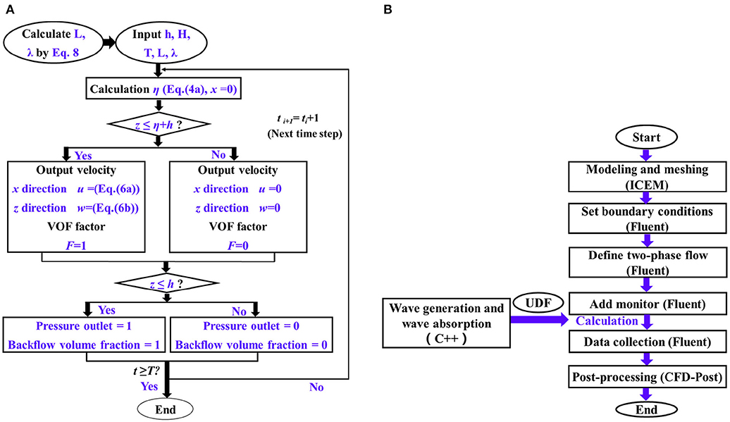
Figure 1. The flowchart for (A) wave generation process; (B) ANSYS/Fluent simulation process.
Waves are generated by applying the boundary wave method at the wave-generating boundary and by specifying the velocity of the fluid in the x and z directions and the instantaneous wave elevation value. Compared to the linear wave theory and to low-order non-linear wave theory, high-order wave theory is more accurate (Zhu, 1983). Therefore, the fifth-order Stokes wave theory as proposed by Skjelbreia and Hendrickson (1960) was used and modeled with the UDF.
The equation providing the instantaneous wave free surface is as below:
where ηn is the waveform coefficient, which is expressed as follows:
where ω is the angular frequency; k is the wave number; h is the water depth; Aij, Bij, and λ are the calculation coefficients determined from c = cosh(kh) and s = sinh(kh) (see section Supplementary Material).
The velocity and instantaneous wave elevation at the wave boundary are as follow:
where is wave celerity, u is the velocity in the x direction, w is the velocity in the z direction and ϕn is the velocity potential function, and its expression is as shown below:
The coefficient λ and wavelength L can be solved using the following transcendental equations:
where L0 is the wavelength in deep waters, H is the wave height (crest to trough height), and C1 and C2 are the calculation coefficient related to c, s, respectively (See section Supplementary Material). In addition, the method proposed by Nishimura et al. (1977) was adopted to correct the coefficient C2 included in the fifth-order Stokes wave formula. The corrected coefficient C2 is given as below:
In order to absorb waves that are reflected at the outlet of the tank, it is necessary to set a wave absorption zone there. A damping term is thus added to the momentum equation for the tank outlet. The momentum equation used is given as follows:
whereu, v, and w are velocity components of the x, y, and z directions; ν is the viscosity coefficient of fluid; α is the coefficient of experience; ρ is fluid density; p is the internal pressure of the fluid; and x1 and x2 are the coordinates of the starting and ending positions of the wave absorption zone, respectively.
Regarding boundary conditions of the numerical tank, the right and upper sides are defined as pressure outlet boundary conditions, the bottom part is defined as the non-slip boundary condition, and the two side boundaries are defined as symmetrical boundaries. The numerical calculation uses a two-phase flow model by adding the water and air phases and uses the volume of fluid (VOF) and geo-reconstruct methods to track the free surface. The discrete form of the pressure term uses the weighted body force, and pressure velocity coupling adopts the pressure solver-based PISO algorithm to obtain a more accurate pressure field and a faster convergence speed (ANSYS, ANSYS). For the interpolation of physical quantities and their derivatives on the control volume interface, we use the second-order upwind format. Since wave motion is a transient process and in order to ensure the accuracy of the calculation and the convergence of the calculation process, the iteration time step should not be excessively large. We adopt a time step of 0.002 s for our study.
We adopt the latest 10-MW large-diameter monopile OWT proposed by the Technical University of Denmark (DTU) (Bak et al., 2013) and apply environmental conditions of characteristic eastern coastal wind farms in China. A 1:25 scale is used to downscale the model and operating environmental conditions with the use of Froude laws. It is stated that this is made in order the computational cost to be smaller. The foundation diameter of the scaled model is set to 0.332 m. To study the influence of a breaking wave on the hydrodynamic performance of the monopile foundation, it is necessary to construct a numerical wave tank with a slope. We developed two bottom slopes. The slope ratio of model 1 is 1:14.15 and extended 16 m in the horizontal direction, and 1.131 m in the vertical direction. The width of the tank is 4 m. The overall layout of the water tank of model 1 is shown in Figure 2A. The slope of model 2 is 1:5.75 and extended 6.5 m in the horizontal direction and 1.31 m in the vertical direction (Figure 2B). The length of the wave absorption zone of both models is more than 1.2 times the wavelength in order to ensure strong wave absorption effects and to limit the influence of reflected waves on the experimental area. In addition, the positioning of the monopile foundation is determined by the breaking point of the wave such that the wave load of the breaking wave relative to the monopile foundation can be measured more accurately.
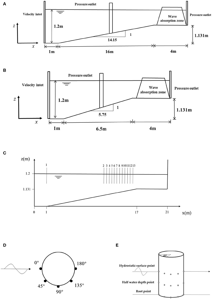
Figure 2. Schematic of the numerical wave tank: (A) Model 1; (B) Model 2; (C) locations of wave gauges; (D) top view of the pressure and wave gauges; (E) front view of the pressure gauges.
In order to measure wave elevation at different places within the numerical wave tank and wave pressure applied at the cylinder wave gauges and pressure gauges have been used, respectively. The wave gauges are arranged at multiple positions on the axis of the water tank to measure the change in the wave height and to determine the positioning of the wave breaking point. The specific plane coordinates of each measuring point are shown in Figure 2C. Measuring point #1 is positioned at the intersection of the plane and slope to verify whether an incident wave is required. Measuring point #1 is 1 m away from the wave generator and point #2 is 14.6 m from the wave generator. As far as the measuring points #2–#13, they are located on the slope and are spaced 0.2 m apart. Moreover, virtual point pressure gauges are placed at the mean water level, at half the water depth and at the bottom of the monopile foundation to measure the instantaneous hydrodynamic pressure. Finally, a virtual wave height gauge system is set on the surface of the monopile foundation to measure the wave run-up value. The configuration of the pressure and wave height gauges is shown in Figure 2D. A front view of the pressure gauge is shown in Figure 2E. Before the simulation, it is necessary to determine the wave breaking point and to accurately measure the wave load.
The type of wave breaking involved is related to the bottom slope ratio and the wave steepness. Therefore, it is necessary to select the appropriate wave characteristics to simulate a breaking wave of the specified form. The type of breaking wave can be distinguished by Irribarren number. The expression of this parameter is as below:
where H0is the height of the deep-water wave, L0 is the wavelength of the deep-water wave and β is the slope of the bottom. In 1968, Galvin (1968) experimentally gave the boundaries of the breaking wave, where ξ0<0.5 defines spilling wave, 0.5 ≤ ξ0 ≤ 3.3 plunging wave and ξ0 >3.3 surging wave.
According to environmental conditions characteristic of China's eastern seas, typical sea conditions are applied, and model conditions are obtained using a scale ratio of 1:25. The examined calculation conditions and relevant information of waves are shown in Table 1, where the Keulegan–Carpenter (KC) number is calculated by the following Equation:
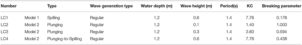
Table 1. Load case for breaking waves.
The mesh of the numerical simulation determines the calculation accuracy and the computational time required. Therefore, we comprehensively consider the computational resources, execution time, and accuracy to determine a suitable and unified meshing scheme to avoid generating a calculation error resulting from a difference in meshing in the simulation of subsequent working conditions. Based on Fifth-Order Stokes wave theory, we identified three meshing schemes for a common rectangular water tank, as shown in Figure 3A. In addition, we use the O-grid form to encrypt along the radial direction close to the monopile to improve the accuracy. The division of mesh used in the tank is illustrated in Figures 3B,C. The detailed information of the three meshing schemes is given in Table 2. The specific wave parameters used are given as follows: the water depth is set to 0.6 m, the wave height is set to 0.08 m, the wave period is set to 1.4 s, and the wavelength is set to 2.77 m. A wave height gauge is placed in the tank 6 meters away from the wave generation boundary to measure wave front patterns.
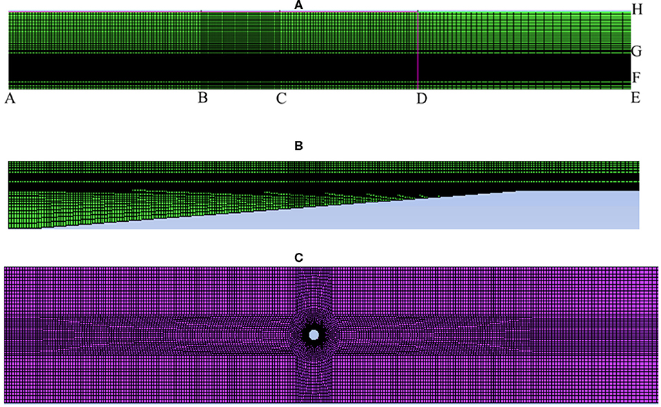
Figure 3. Schematic diagram of mesh, (A) meshing schemes; (B) numerical wave tank: side view; (C) numerical wave tank: top view.
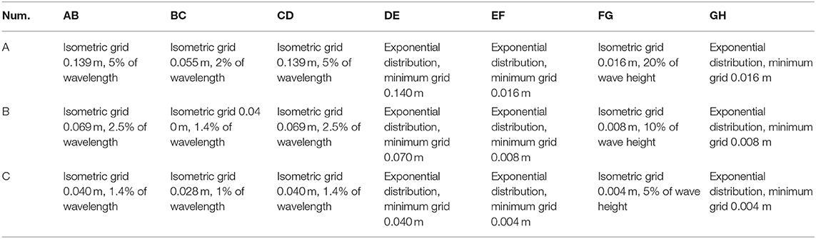
Table 2. Meshing schemes.
To determine the validity of the numerical wave tank, we compare the measured wave front with the theoretical Fifth-order Stokes wave values based on the same wave characteristics. The results are shown in Figures 4A–C; the wave front of scheme A differs greatly from the theoretical value measured at the wave trough, which will introduce errors into the subsequent calculations. Thus, scheme A is rejected. The wave front curves of schemes B and C are in good agreement with the theoretical values, meeting the calculation requirements. Although the meshing of scheme C is more precise, we observe no significant improvements in simulation accuracy, and we find a considerable increase in the number of grids, resulting in a decline in computational efficiency. Therefore, the subsequent simulations presented in this paper use scheme B as the basis for the mesh division. Forty grids are divided into one wavelength in the horizontal direction, and 10 grids are divided into one wave height in the vertical direction. To further verify the accuracy of scheme B, we perform a corresponding spectrum analysis on the simulated wave front curve (Figure 4D). A comparison of the spectra shows that the spectrum that corresponds to scheme B agrees well with the theoretical values for each order peak, revealing obvious non-linear characteristics.
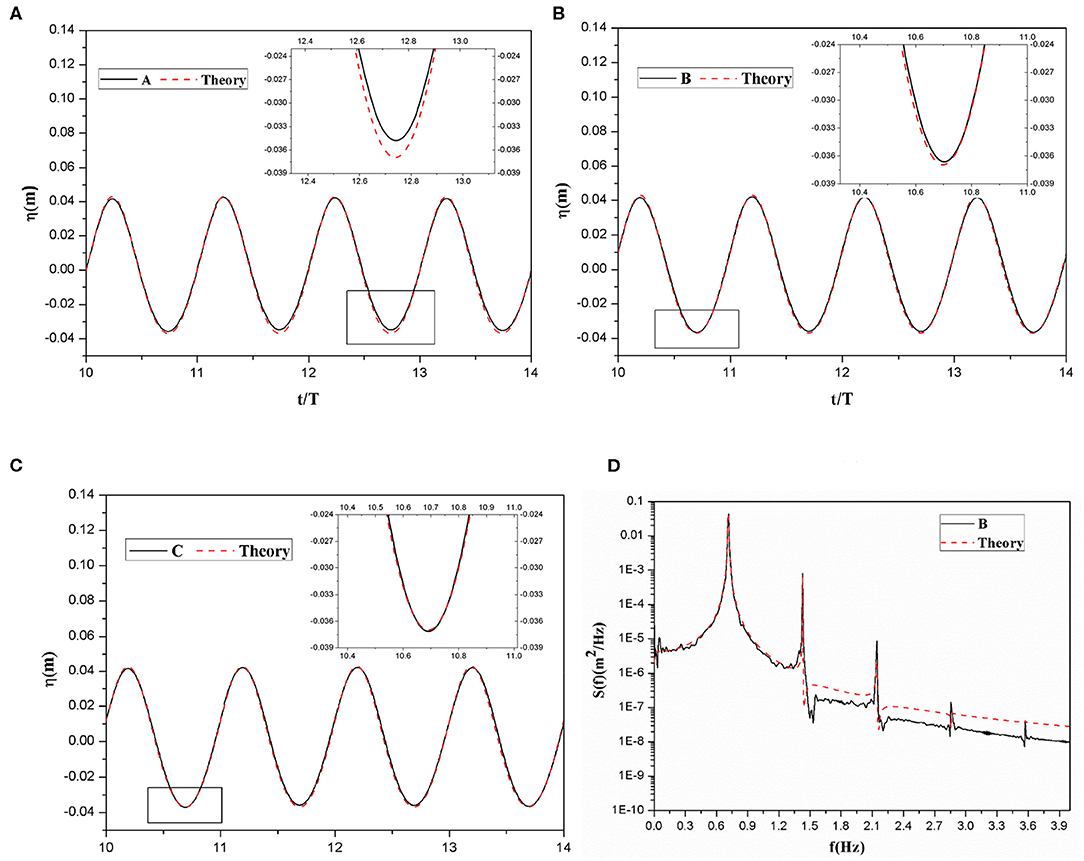
Figure 4. Comparison of wave elevation measured from the numerical tank and theoretical values: (A) scheme A; (B) scheme B; (C) scheme C; (D) Spectrum of scheme B.
The validity of using a numerical tank to study the hydrodynamic loads of a monopile foundation is presented here. OC5 monopile OWT model test data (Robertson et al., 2016) are compared against the numerical simulation predictions of the present work. The overall layout and working conditions of a water tank should be consistent with those of the model. The diameter of the foundation is set to 0.075 m, the water depth 0.78 m, the wave height 0.09 m and the wave period 1.5655 s. A slope of 1:25 is formed in front of the wave generator extending to a plateau. The cylinder is placed on the slope 7.75 m away from the wave generator. The overall layout of the numerical wave tank is shown in Figure 5A. In Figure 5B, a comparison between OC5 model test data and numerical simulation predictions of the numerical wave tank is presented. The figure shows strong agreement at the wave crest, and numerical simulation results for the trough are slightly lower in value than the data derived from the model test. This difference is mainly observed because a different wave theory is applied. Based on the presented data and using the methods described above, the numerical simulation presented in this paper ensures the accuracy of both calculated and maximum responses so that the numerical wave tank can be used for subsequent simulations.
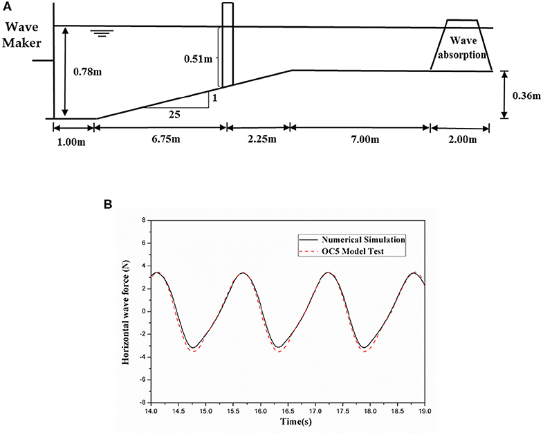
Figure 5. OC5 project: (A) Side view of the water tank and cylinder location. (B) Compare numerical simulation results to OC5 model test results.
This section mainly examines the influence of a spilling breaking wave under different breaking parameters ξ0 on wave run-up, pressure and horizontal wave force around the monopile foundation and then explores laws governing how the spilling breaking wave affects the hydrodynamic performance of a large-scale monopile OWT. The foundation of the 10 MW monopile OWT is taken as the research object, and LC1 is used to carry out the simulation (Table 1). Under this load case, the bottom slope ratio is set 1:14.15, the water depth is set 1.2 m, the wave height 0.6 m and the period 1.4 s. The wave breaking parameter equals to 0.402 and a spilling wave is generated. Before the simulation, it is necessary to find the wave breaking point to determine the positioning of the monopile and to accurately measure the wave loads. The specific method used is the same as that described in previous section and is thus not described here. Finally, the coordinate of the breaking point is set as 1.9 m.
Figure 6A shows the wave run-up of the 0°, 45°, 90°, 135°, and 180° gauge directions of the monopile foundation surface. The figure shows that the run-up law of the wave under the combination is basically the same as that of combination one and a second peak is generated. However, as the incident wave height increases, the run-up value also increases accordingly. In addition, several small peaks appear in the run-up time series curve of the 90° gauge direction, and those small peaks are densely distributed. This shows that the wave is superimposed multiple times in this direction for a short period, after which and then several small peaks are formed.
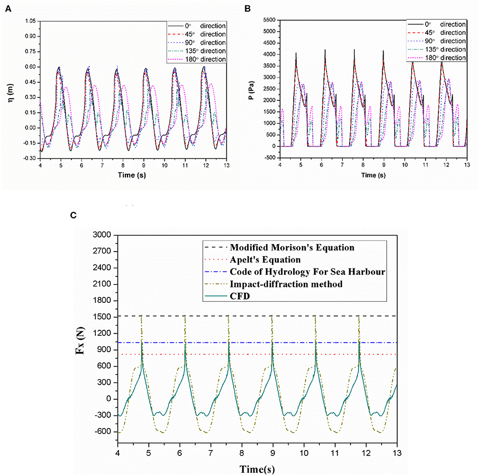
Figure 6. (A) Wave run-up; (B) pressure; (C) wave force (ξ0 = 0.178).
Figure 6B shows pressure time series of the 0°, 45°, 90°, 135°, and 180° gauge directions for the still water surface of the monopile foundation under the action of a breaking wave (ξ0 = 0.178). The spilling breaking wave with breaking parameter (ξ0 = 0.178) not only causes the monopile foundation to generate a larger pressure value in the 0° direction but also causes the pressure time series of the 0° direction to reach double peaks. In addition, we found that the positioning of the maximum pressure drops rapidly in the upper section from 90° to 135°. Under these conditions, the pressure drops rapidly during wave propagation from 45° to 90°, while the maximum pressure recorded at 90° and 135° is not considerable different. This is mainly attributed to the fact that for more gradual waves, the non-linear action of the waves is mainly reflected in front of the monopile. With an increase in wave steepness and non-linearity, the influence of waves on the back end of monopile grows more significant. Although waves bypass the monopile during propagation, their effect on the foundation continues and does not immediately decline. From the long and high water ridge on the back of the monopile foundation, we find that the steep breaking wave has a stronger influence on the back end of the foundation. In addition, the pressure time series of the 135° and 180° gauge directions form different shapes under the two load cases further illustrating this pattern.
Figure 6C presents the time series curve of the horizontal wave force acting on the monopile foundation for ξ0 = 0.178. The figure shows that the curve at the peak is steep and sharp, and the degree of non-linearity observed is high. The calculated with the CFD model force has been compared with relevant results calculated with analytical formulas as below.
According to experimental and Morison equations, the US Coastal Engineering Research Center has developed the Modified Morison's equation for calculating the maximum breaking force (Xu, 2004):
where Hb is the breaking wave height and D is the pile diameter.
The empirical equation for calculating the breaking force obtained from Apelt's equation (Apelt and Piorewicz, 1987) is written as:
where H0 is the deep water wave height and L0 is the deep water wave length.
China's “Code of Hydrology for Sea Harbor” (Ministry of Transportation and Communications, 2013) also provides a means of calculation the maximum breaking force of an upright pile in a shallow water area:
where A, B1, B2 is the test coefficient, A and B1 are determined by the bottom slope ratio, and B2 equals to 0.35. According to the specifications, we apply A = 0.48 and B1 = −0.44.
The impact-diffraction method provides an equation for solving the breaking force (Goda et al., 1966; Wienke and Oumeraci, 2005).
where db is the water depth in front of pile, D is the pile diameter, u is water particle velocity, CM and CD are force coefficients, Cs is the slamming coefficient, λ is the curling factor, T is the time duration and ηb, ρ, R, and t are wave elevation, water density, pile radius and time, respectively. The solution value of the equation is related to the selection of those parameters. According to the range given by the parameter, we select λ = 0.4, Cs = π, (Goda et al., 1966) and ρ = 998kg/m3. The impact velocity impact elevation ηb is extracted from the CFD simulation.
The maximum horizontal wave force of the monopile foundation is roughly 1030.02 N, and the wave force calculated with the conventional Morison equation according to the water depth and wave height is only 467.46 N. We can conclude that the conventional Morison equation is not suitable for calculating the breaking wave force for those conditions. The breaking wave force calculated using the impact-diffraction method (1540.815 N) and the modified Morison equation (1523.535 N) are relatively close and significantly larger than the other three. Therefore, the applicability of the modified Morison equation must be considered when calculating the breaking wave force of a steep wave. The breaking wave force calculated with Apelt's equation (823.771 N) is less than that calculated from the Code of Hydrology for Sea Harbor and from CFD. Results generated from the Code of Hydrology for Sea Harbor (1034.530 N) and via CFD are basically the same with minor differences.
Figure 7 shows the flow of the breaking wave along the monopile foundation for the case of breaking parameter ξ0= 0.178. The figure shows the displacement contour plot of the vertical direction and demonstrates that the wave is steepen under these conditions and is more upright and steep when it breaks. During interactions with the monopile foundation, the wave around the monopile shows obvious signs of upwelling. In addition, a long and high water ridge can be clearly observed on the back surface of the monopile foundation, which has presents non-linear characteristics.
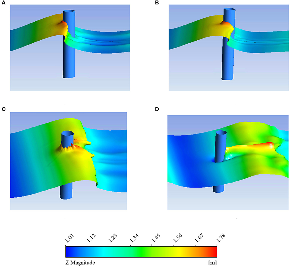
Figure 7. Breaking wave (ξ0 = 0.178) flow around the monopile foundation. (A) time = 9 s; (B) time = 9.16 s; (C) time = 9.48 s; (D) time = 9.96 s.
This section mainly explores the influence of plunging breaking waves under different breaking parameters ξ0 on the wave run-up, pressure and the horizontal wave force around the monopile foundation and then studies the influence of plunging breaking waves on the hydrodynamic performance of the large-scale monopile OWT.
This section extends our simulation by applying LC2 from Table 1. For model 2 in LC2, the bottom slope ratio equals to 1:5.75, the water depth is set as 1.2 m, the wave height 0.1 m and the period 1.4 s. The wave breaking parameter equals to 1.000 and plunging waves are generated. The wave breaking point coordinate equals to 7.4 m.
The center of the monopile foundation is placed at 7.4 m. Figure 8A shows the wave run-up in the 0°, 45°, 90°, 135°, and 180° gauge directions for the monopile foundation surface along the wave propagation direction. The figure shows that the surface elevation curve of the plunging wave is more disordered than that of the spilling wave, and irregularities and multi-peak phenomena appear in the curves in all directions. This mainly occurs because under the same load case, as the bottom slope ratio increases, the non-linear growth rate of the wave increases, generating a steep front slope, forward tilting and rapid rollover. A small volume of air is involved in this process, and interactions occurring between the breaking waves and the monopile foundation enhance the non-linear characteristics, which in turn causes the wave surface to become more disordered.
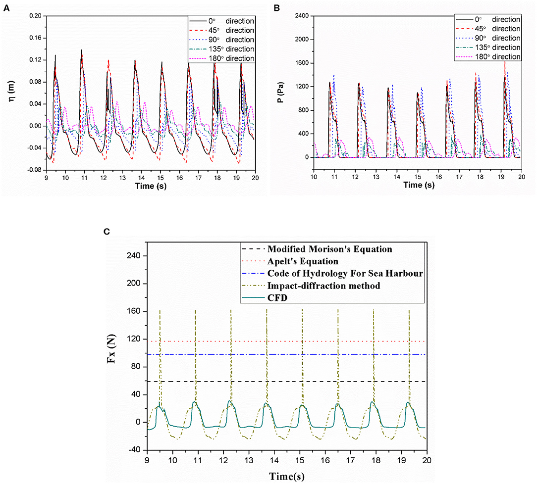
Figure 8. (A) Wave run-up; (B) pressure; (C) wave force (ξ0 = 1.000).
Figure 8B shows pressure time series of the 0°, 45°, 90°, 135° and 180° gauge directions for the still water surface of the monopile foundation under the action of a breaking wave (ξ0 = 1.000). The plunging breaking wave with breaking parameter (ξ0 = 1.000) causes the monopile foundation to generate a much lower pressure value compared with the spilling wave with ξ0 = 0.178. The pressures at 135° and 180° are significantly lower than 0°, 45° and 90° direction.
In Figure 8C the time series curve of the horizontal wave force acting on the monopile foundation when ξ0 = 1.000 is presented. The figure shows that the maximum horizontal wave force of the monopile foundation reaches roughly 31.353 N. Results derived from CFD and different methods for solving wave breaking wave forces are compared in Figure 8C. It shows that the wave breaking wave force, in this case, varies considerably when using different methods. Since Apelt's equation (117.071 N) does not take into account the influence of the slope of the water, the calculated value is the same as the value of the spilling wave for the same load case. In this case, the value calculated via CFD is relatively small, and a certain degree of error may be involved. The values calculated from Modified Morison's Equation equals 58.995 N whereas the Code of Hydrology for Sea Harbor gives a value of 98.126 N, while, the impact-diffraction method predicts the highest value (163.113 N).
Figure 9 shows the flow run-up of the breaking wave along the monopile foundation for breaking parameter ξ0 = 1.000. The figure shows the displacement contour plot for the vertical direction. Compared to the contour plot of the spilling wave, the displacement contour plot, in this case, is mainly reflected at the back of the monopile foundation. As is shown in Figure 9C, after the waves interact with the monopile, the waves continue to propagate and form two water heads on the back side of the monopile rather than immediately fusing to form a ridge. This mainly occurs because, under this combination, the wave breaking point is positioned rearward and closer to the flat slope behind. After the wave bypasses the pile, limited by the flat slope and water depth, after breaking the wave no longer moves intensely and cannot converge on the back of the monopile causing two water heads to form as the wave continues to propagate. For ξ0 = 1.000 all the analytical equations overpredict the maximum hydrodynamic load.
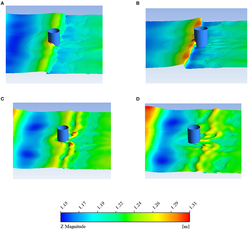
Figure 9. Breaking waves (ξ0 = 1.000) flow around the monopile foundation. (A) time = 12.24 s; (B) time = 12.4 s; (C) time = 12.56 s; (D) time = 12.72 s.
This section extends the simulation by applying LC3. Under this load case, the bottom slope ratio equals to 1:5.75, the water depth is set to 1.2 m, the wave height 0.3 m and the period 1.4 s. The wave breaking parameter equals to 0.594 and plunging waves are generated. The wave breaking point coordinate is set to 5.7 m.
The center of the monopile foundation is established at 5.7 m to measure relevant parameters such as the wave loads. Figure 10A shows the wave run-up for the 0°, 45°, 90°, 135°, and 180° directions for the monopile foundation surface along the wave propagation direction. The figure shows that the wave surface elevation curve in the 90° and 135° directions is still turbulent and irregular in shape, showing that air is carried as the plunging wave breaks.
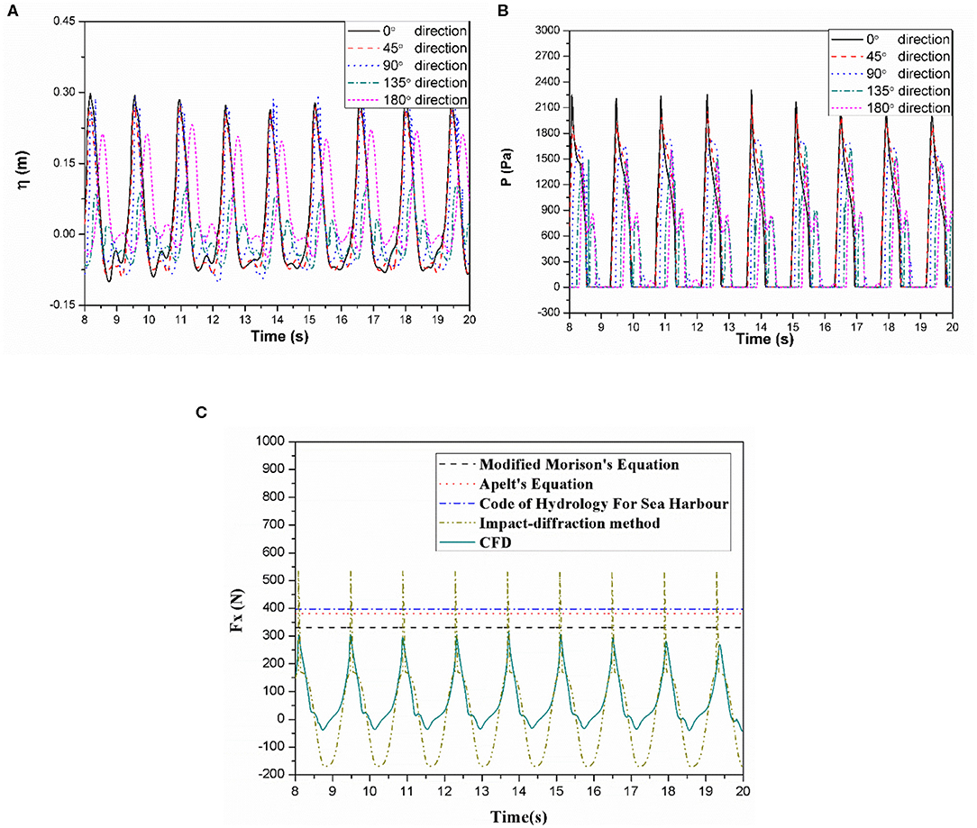
Figure 10. (A) Wave run-up; (B) pressure; (C) wave force (ξ0 = 0.594).
Figure 10B shows the pressure time series in the 0°, 45°, 90°, 135°, and 180° directions for the still water surface of the monopile foundation under the action of breaking waves (ξ0 = 0.594). Under this condition, in addition to a relatively steep secondary peak appearing in the 135° direction, small peaks appear along horizontal straight lines of the 90° and 180° directions as shown in Figure 10B. However, this phenomenon does not appear during the simulation of the spilling waves. The presence of this horizontal straight line is mainly attributed to the fact that as the trough acts on the monopile foundation, the pressure gauge on the hydrostatic surface does not come into contact with the water, and the pressure value is not detected. Thus, the partial value of the pressure time series at the hydrostatic surface is zero. Under the action of plunging waves, even when the trough acts on the monopile foundation, the pressure gauge of the 90° direction and the 180° direction hydrostatic surface come into contact with the water and generate a certain pressure value, showing that the plunging wave has a stronger non-linear effect. When studying the effects of plunging wave pressure on the foundation, they cannot be simply calculated from the law of a traveling wave.
Figure 10C presents the time series curve of the horizontal wave force acting on the monopile foundation when ξ0 = 0.594. The figure shows that the maximum horizontal wave force of the monopile foundation is calculated approximately with a value equals to 313.446 N. The results of different methods used to solve the breaking wave force in this work are also compared in Figure 10C. The figure shows that the breaking wave forces calculated with several methods (Modified Morison's Equation gives 331.368 N, Apelt's Equation gives 381.152 N, Code of Hydrology for Sea Harbor gives 396.790 N and the impact-diffraction method gives 533.813 N) under this condition are not considerably different, showing that the calculation results are more accurate, but again the analytical solutions overpredict the maximum hydrodynamic load.
Figure 11 presents a displacement contour plot of the flow around the breaking wave when ξ0 = 0.594. The figure shows that the forward deflection and curling of the breaking wave are more severe in the case of large and steep wave. Moreover, the breaking point is located far from the rear flat slope and without the influence of the flat slope; a water ridge appears at the back of the monopile foundation.
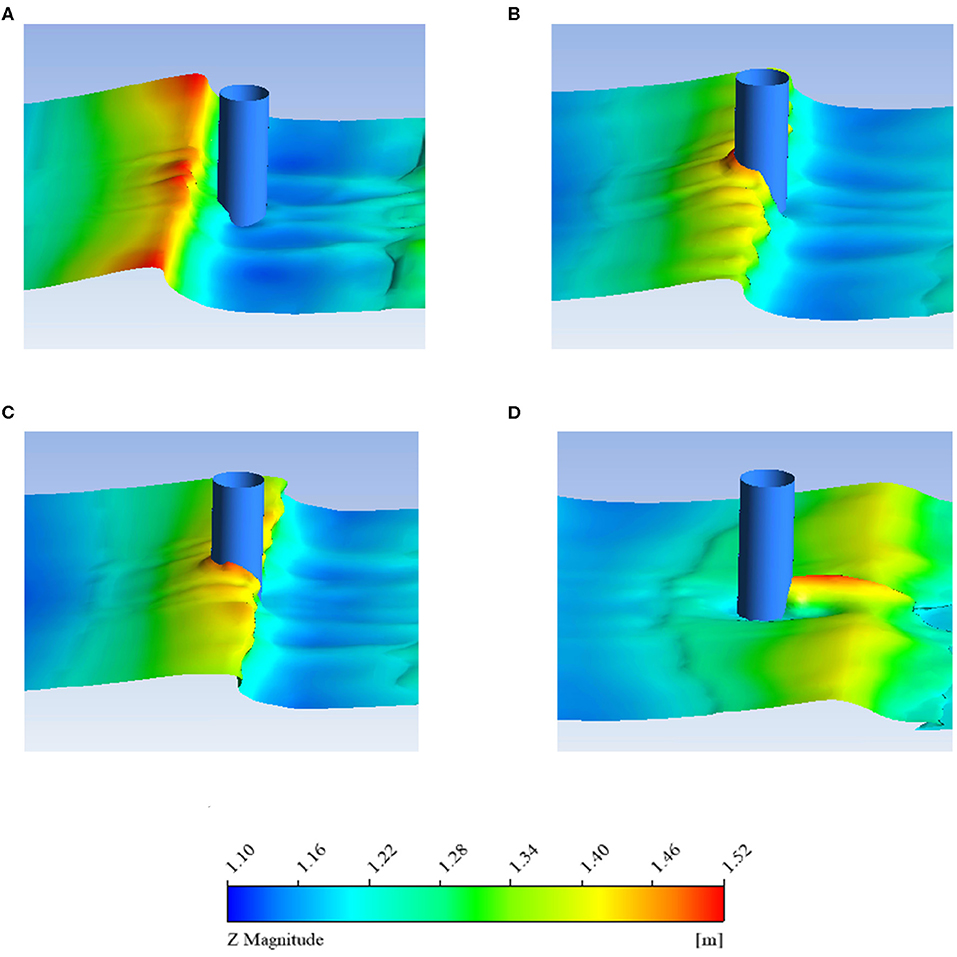
Figure 11. Breaking wave (ξ0 = 0.594) flow around the monopile foundation. (A) time = 10.68 s; (B) time = 11 s; (C) time = 11.08 s; (D) time = 11.32 s.
When the slope of the base remains unchanged with an increase in wave height the breaking parameters of the wave changes and the breaking form transits from plunging to spilling waves. In view of this physical condition, this section extends the simulation by applying LC4. Under this condition, the bottom slope ratio is 1:5.75, the water depth is set as 1.2 m, the wave height is set as 0.6 m and the period is set as 1.4 s. The wave breaking parameter is set as 0.438 and plunging waves are generated. The wave breaking point coordinate is 1.2 m.
The center of the monopile foundation is defined at 1.2 m to measure relevant parameters such as wave loads. Figure 12A shows the wave run-up in the 0°, 45°, 90°, 135°, and 180° directions for the monopile foundation surface along the wave propagation direction. The figure shows that while the wave steepness increases in this section, the wave surface elevation curve is not more disordered but is instead more consistent than that described in the above section. This shows that the intensity of interactions occurring between the breaking wave and monopile foundation mainly depends on the form of wave breaking involved while the relationship to wave steepness is weak.
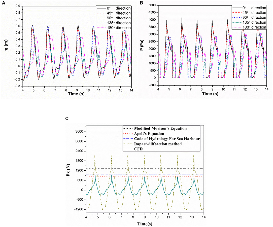
Figure 12. (A) Wave run-up; (B) pressure; (C) wave force (ξ0 = 0.438).
Figure 12B shows the pressure time series of the 0°, 45°, 90°, 135°, and 180° gauge directions for the still water surface of the monopile foundation under the action of breaking wave (ξ0 = 0.438). The figure shows that the pressure time series curve observed under this condition is much smoother than that of the plunging wave with no sharp peak. We also find that the rapid drop in pressure observed under this condition occurs during the propagation of waves from 45° to 90° while the maximum pressure values at 90° and 135° are not much different. These patterns are the same as those observed from the spilling waves with breaking parameter ξ0 = 0.178 described above. We further observed that the steeper the waves become the more non-linear the waves are, and the impact on the back of the monopile becomes larger as a result.
Figure 12C shows the time series curve of the horizontal wave force acting on the monopile foundation when ξ0 = 0.438. The figure shows that the maximum horizontal wave force of the monopile foundation is roughly 878.367 N. The comparative results of this work and different methods for solving breaking wave forces are also compared in Figure 12C. It shows that values of the breaking force calculated from Apelt's equation (823.771 N), the Code of Hydrology for Sea Harbor (980.405 N) and the CFD are relatively close. However, as the value calculated from the impact-diffraction method (2153.844 N) and the modified Morison equation (1338.725 N) are large, it is necessary to consider its applicability in the midst of large and steep waves.
Figure 13 presents a displacement contour plot of the breaking wave flow observed around the monopile foundation with a breaking parameter of ξ0 = 0.438, The figure shows that the wave flow around the monopile foundation is similar to that observed from the spilling wave of breaking parameter ξ0 = 0.178 described in combination two. The incident wave height and period are the same, and both are breaking forms of spilling waves, exhibiting certain similarities.
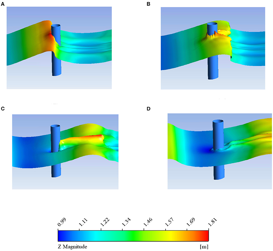
Figure 13. Breaking wave (ξ0 = 0.438) flow around the monopile foundation. (A) time = 9 s; (B) time = 9.48 s; (C) time = 9.8 s; (D) time = 10.12 s.
In this paper, we developed a numerical wave tank that can explore the effect of breaking waves of different type on the foundation of a 10 MW monopile OWT. In order we to model the wave propagation a user-defined function was developed, validated and used for the numerical modeling of the waves within the tank based on Fifth-Order Stokes wave theory. Moreover, the developed numerical wave tank has been validated for ensuring its effectiveness for producing correct results. Spilling and plunging breaking waves were generated in the numerical wave tank with different bottom slopes. The effects of spilling and plunging breaking waves on the wave run-up height, pressure and horizontal wave force on a 10 MW monopile foundation are investigated. Different analytical methods for calculating the wave breaking loads are compared with the developed computational fluid dynamics model and their differences are quantified and discussed. The main findings of our study are as below:
(1) The maximum wave run-up peak caused by a breaking wave represents a large proportion of the whole wave height, and especially for the wave front surface of the monopile foundation, the performance is more pronounced. The reverberating side wave generated by a breaking wave will create a secondary peak or even a tertiary peak around the monopile foundation. Because plunging wave breaking is accompanied by the entrapment of air, the surface elevation curve of a plunging wave is more disordered than that of a spilling wave, and irregularities and multi-peak phenomena appear in curves in all directions. In addition, we use control variables to explore factors that affect the non-linearity of the surface elevation around the monopile foundation. We find that the intensity of interactions occurring between the breaking wave and the foundation depends mainly on the form of wave breaking involved and the relationship to wave steepness is weak.
(2) Pressure acting on the foundation obtains its largest values along the front surface (0° gauge direction). For less steep waves, a sudden drop in pressure occurs between 90° and 135° direction. For steeper waves, a sudden drop in pressure value occurs between 45° and 90°, and pressure levels are basically the same or undergo minor changes between 90° and 180°. This shows that for a less steep wave, the non-linear effect of such a wave is mainly reflected in the front of the pile. A steeper wave instead has a stronger influence on the back of the pile. In addition, due to the high degree of non-linearity of breaking waves, a steep secondary peak appears in the pressure time series curve, exhibiting highly non-linear characteristics. Under the action of a plunging wave, even when the trough acts on the monopile foundation, the pressure gauge at the hydrostatic surface also come into contact with the water and generates a certain pressure value, indicating that the non-linear effect of the plunging wave is strong. The effect of pressure from the plunging wave on the pile cannot be simply calculated from basic analytical solutions.
(3) The wave load created by a breaking wave is larger than that created by a traveling wave under the same load conditions. Using the conventional Morison equation to calculate the breaking force will generate a smaller value. In shallow water, the conventional Morison equation should be used with caution to calculate the breaking force acting on the foundation. The modified Morison equation increases the accuracy of calculation results to a certain extent, but the calculation of the breaking wave force under a steep wave will still produce a large error value. In addition, the bottom slope ratio has a certain influence on the calculation of the breaking wave force, but the effect is minor. Apelt's equation does not take into account the influence of the bottom slope ratio, and the coefficient can be corrected accordingly to different situations. In this paper, the breaking wave force calculated by CFD is generally reasonable, but the calculated value is relatively small for less steep waves.
(4) For spilling breaking waves, modified Morison equation is giving 1.48 times (ξ0 = 0.178) larger maximum value of the impact load compared to the CFD; Apelt's Equation gives 0.80 times (ξ0 = 0.178) larger maximum value of the impact load compared to the CFD; Code of Hydrology for Sea Harbor gives 1.0 times (ξ0 = 0.178) larger maximum value of the impact load compared to the CFD.
(5) For plunging breaking waves, modified Morison equation is giving 1.88 times (ξ0 = 1.000) and 1.05 times (ξ0 = 0.594) larger maximum value of the impact load compared to the CFD; Apelt's Equation gives 3.73 times (ξ0 = 1.000) and 1.22 times (ξ0 = 0.0.594) larger maximum value of the impact load compared to the CFD; Code of Hydrology for Sea Harbor gives 3.13 times (ξ0 = 1.000) and 1.26 times (ξ0=0.594) larger maximum value of the impact load compared to the CFD.
All datasets generated for this study are included in the article/Supplementary Material.
WS, DN, and CM: conceptualization. WS, YT, DN, and CM: methodology. YT, WS, DN, and CM: investigation. YT, JY, WS, and CM: writing—first draft preparation. WS, JY, DN, and CM: writing, review, and editing. YT: visualization. WS: supervision. All authors contributed to the article and approved the submitted version.
This research was funded by the international collaboration and exchange program from the NSFC-RCUK/EPSRC with Grant No. 51761135011. This work is also supported by the National Natural Science Foundation of China (Grant Nos. 51709039 and 51709040). This work is also partially supported by LiaoNing Revitalization Talents Program (XLYC1807208) and the Fundamental Research Funds for the Central University (DUT19GJ209).
YT was employed by the company China Water Northeastern Investigation, Design & Research Co., Ltd.
The remaining authors declare that the research was conducted in the absence of any commercial or financial relationships that could be construed as a potential conflict of interest.
The Supplementary Material for this article can be found online at: https://www.frontiersin.org/articles/10.3389/fmars.2020.00427/full#supplementary-material
Aggarwal, A., Chella, M. A., Bihs, H., and Arntsen, Ø. A. (2017). Numerical study of irregular breaking wave forces on a monopile for offshore wind turbines. Energ. Proc. 137, 246–254. doi: 10.1016/j.egypro.2017.10.347
Apelt, C. J., and Piorewicz, J. (1987). Laboratory studies of breaking wave forces acting on vertical cylinders in shallow water. Coast. Eng. 11, 263–282. doi: 10.1016/0378-3839(87)90015-9
Bachynski, E. E., and Ormberg, H. (2015). “Hydrodynamic modeling of large-diameter bottom-fixed offshore wind turbines,” in Proceedings of the ASME (2015). 34th International Conference on Ocean, Offshore and Arctic Engineering (OMAE 2015) (St. John's, NL).
Bak, C., Zahle, F., Bitsche, R., Kim, T., Yde, A., Henriksen, L. C., et al. (2013). The DTU 10-MW reference wind turbine. Danish Wind Power Res. 2013.
Bredmose, H., and Jacobsen, N. G. (2010). “Breaking wave impacts on offshore wind turbine foundations: focused wave groups and CFD,” in Proceedings of the ASME (2010). 29th International Conference on Ocean, Offshore and Arctic Engineering (OMAE 2010) (Shanghai).
Chella, M. A., Bihs, H., and Myrhaug, D. (2019). Wave impact pressure and kinematics due to breaking wave impingement on a monopile. J. Fluids Struc. 86, 94–123. doi: 10.1016/j.jfluidstructs.2019.01.016
Chen, X. B., Li, J., and Chen, J. Y. (2011). Calculation of the nonlinear wave force of offshore wind turbine based on the stream function wave theory. J. Hunan Univ. Nat. Sci. 38, 22–28.
Choi, S. J., Lee, K. H., and Gudmestad, O. T. (2015). The effect of dynamic amplification due to a structures vibration on breaking wave impact. Ocean Eng. 96, 8–20. doi: 10.1016/j.oceaneng.2014.11.012
Esteban, M. D., López-Gutiérrez, J. S., Diez, J. J., and Negro, V. (2011). Offshore wind farms: foundations and influence on the littoral processes. J. Coast. Res. 64, 656–660. Available online at: http://www.cerf-jcr.org/images/stories/2011_ICS_Proceedings/SP64_656-660_M.D.Esteban.pdf
Europe, W. (2019). Offshore Wind in Europe: Key Trends and Statistics (2018). Brussels: Wind Europe.
Galvin, C. J. (1968). Breaker type classification on three laboratory beaches. J. Geophys. Res. 73, 3651–3659. doi: 10.1029/JB073i012p03651
Ghadirian, A., and Bredmose, H. (2019). Pressure impulse theory for a slamming wave on a vertical circular cylinder. J. Fluid Mechan. 867, 1–14. doi: 10.1017/jfm.2019.151
Ghadirian, A., and Bredmose, H. (2020). Detailed force modelling of the secondary load cycle. J. Fluid Mechan. 889, 1–30. doi: 10.1017/jfm.2020.70
Goda, Y., Haranaka, S., and Kitahata, M. (1966). Study of impulsive breaking wave forces on piles. Rep. Port Harbour Techn. Res. Inst. 6, 1–30.
Hirt, C. W., and Nichols, B. D. (1981). Volume of fluid (VOF) method for the dynamics of free boundaries. J. Comput. Phys. 39, 201–225. doi: 10.1016/0021-9991(81)90145-5
Jose, J., Choi, S. J., Giljarhus, K. E. T., and Gudmestad, O. T. (2017). A comparison of numerical simulations of breaking wave forces on a monopile structure using two different numerical models based on finite difference and finite volume methods. Ocean Eng. 137, 78–88. doi: 10.1016/j.oceaneng.2017.03.045
Liu, S., Jose, J., Ong, M. C., and Gudmestad, O. T. (2019). Characteristics of higher-harmonic breaking wave forces and secondary load cycles on a single vertical circular cylinder at different Froude numbers. Marine Struc. 64, 54–77. doi: 10.1016/j.marstruc.2018.10.007
Marino, E., Borri, C., and Lugni, C. (2011a). Influence of wind-waves energy transfer on the impulsive hydrodynamic loads acting on offshore wind turbines. J. Wind Eng. Ind. Aerod. 99, 767–775. doi: 10.1016/j.jweia.2011.03.008
Marino, E., Borri, C., and Peil, U. (2011b). A fully nonlinear wave model to account for breaking wave impact loads on offshore wind turbines. J. Wind Eng. Ind. Aerod. 99, 483–490. doi: 10.1016/j.jweia.2010.12.015
Marino, E., Lugni, C., and Borri, C. (2013a). A novel numerical strategy for the simulation of irregular nonlinear waves and their effects on the dynamic response of offshore wind turbines. Comput. Methods Appl. Mechan. Eng. 255, 275–288. doi: 10.1016/j.cma.2012.12.005
Marino, E., Lugni, C., and Borri, C. (2013b). The role of the nonlinear wave kinematics on the global responses of an OWT in parked and operating conditions. J. Wind Eng. Ind. Aerod. 123, 363–376. doi: 10.1016/j.jweia.2013.09.003
Marino, E., Nguyen, H., Lugni, C., Manuel, L., and Borri, C. (2015). Irregular nonlinear wave simulation and associated loads on offshore wind turbines. J. Offshore Mechan. Arctic Eng. 137:021901. doi: 10.1115/1.4029212
Ministry of Transportation and Communications (2013). Industry Standard of the PRC: Code of Hydrology for Sea Harbor (JTS 145–2–2013). Beijing: China Communications Press.
Mockute, A., Marino, E., Lugni, C., and Borri, C. (2019). Comparison of nonlinear wave-loading models on rigid cylinders in regular waves. Energies 12:4022. doi: 10.3390/en12214022
Myrhaug, D., and Holmedal, L. E. (2010). Wave run-up on slender circular cylindrical foundations for offshore wind turbines in nonlinear random waves. Coast. Eng. 57, 567–574. doi: 10.1016/j.coastaleng.2009.12.003
Nishimura, H., Isobe, M., and Horikawa, K. (1977). Higher order solutions of the stokes and the cnoidal waves. J. Fac. Eng. Univ. Tokyo Ser. B 2, 267–293.
Paulsen, B. T., Bredmose, H., Bingham, H. B., and Jacobsen, N. G. (2014). Forcing of a bottom-mounted circular cylinder by steep regular water waves at finite depth. J. Fluid Mechan. 755, 1–34. doi: 10.1017/jfm.2014.386
Robertson, A. N., Wendt, F., Jonkman, J. M., Popko, W., Borg, M., Bredmose, H., et al. (2016). OC5 project phase Ib: validation of hydrodynamic loading on a fixed, flexible cylinder for offshore wind applications. Energ. Proc. 94, 82–101. doi: 10.1016/j.egypro.2016.09.201
Schløer, S., Bredmose, H., and Bingham, H. B. (2016). The influence of fully nonlinear wave forces on aero-hydro-elastic calculations of monopile wind turbines. Marine Struc. 50, 162–188. doi: 10.1016/j.marstruc.2016.06.004
Shi, W., Park, H. C., Chung, C. W., and Kim, Y. C. (2011). “Comparison of dynamic response of monopile, tripod and jacket foundation system for a 5-MW wind turbine,” in Proceedings of the 21st International Offshore and Polar Engineering Conference (Honolulu, HI: International Society of Offshore and Polar Engineers).
Skjelbreia, L., and Hendrickson, J. (1960). “Fifth order gravity wave theory,” in Proceedings of the 7th Coastal Engineering Conference (Hague).
Vos, L. D., Frigaard, P., and Rouck, J. D. (2007). Wave run-up on cylindrical and cone shaped foundations for offshore wind turbines. Coast. Eng. 54, 17–29. doi: 10.1016/j.coastaleng.2006.08.004
Wienke, J., and Oumeraci, H. (2005). Breaking wave impact force on a vertical and inclined slender pile-theoretical and large-scale model investigations. Coast. Eng. 52, 435–462. doi: 10.1016/j.coastaleng.2004.12.008
Wind Power Offshore (2013). In Depth: Cost Imperative Drives Monopiles to New Depths. Available online at: http://www.windpoweroffshore.com/article/1210058/depth-cost-imperativedrives-monopiles-new-depths
Xu, X. P. (2004). Breaking wave forces on the vertical cylinders. J. China University of Petroleum 28, 80–82.
Zhou, H., and Wan, D. C. (2014). Numerical simulation of the unsteady flow around wind turbines with different blades numbers. Chin. J. Hydrodyn. 29, 444–453. doi: 10.3969/j.issn1000-4874.2014.04.009
Keywords: offshore wind turbines, large diameter monopile, fifth-order stokes waves, hydrodynamic analysis, breaking waves, wave loads
Citation: Tang Y, Shi W, Ning D, You J and Michailides C (2020) Effects of Spilling and Plunging Type Breaking Waves Acting on Large Monopile Offshore Wind Turbines. Front. Mar. Sci. 7:427. doi: 10.3389/fmars.2020.00427
Received: 04 February 2020; Accepted: 14 May 2020;
Published: 19 June 2020.
Edited by:
Eugen Victor Cristian Rusu, Dunarea de Jos University, RomaniaReviewed by:
Enzo Marino, University of Florence, ItalyCopyright © 2020 Tang, Shi, Ning, You and Michailides. This is an open-access article distributed under the terms of the Creative Commons Attribution License (CC BY). The use, distribution or reproduction in other forums is permitted, provided the original author(s) and the copyright owner(s) are credited and that the original publication in this journal is cited, in accordance with accepted academic practice. No use, distribution or reproduction is permitted which does not comply with these terms.
*Correspondence: Wei Shi, d2Vpc2hpQGRsdXQuZWR1LmNu; Dezhi Ning, ZHpuaW5nQGRsdXQuZWR1LmNu
Disclaimer: All claims expressed in this article are solely those of the authors and do not necessarily represent those of their affiliated organizations, or those of the publisher, the editors and the reviewers. Any product that may be evaluated in this article or claim that may be made by its manufacturer is not guaranteed or endorsed by the publisher.
Research integrity at Frontiers
Learn more about the work of our research integrity team to safeguard the quality of each article we publish.