Data-Driven Modeling of Global Storm Surges

In many areas, storm surges caused by tropical or extratropical cyclones are the main contributors to critical extreme sea level events. Storm surges can be simulated using numerical models that are based on the underlying physical processes, or by using data-driven models that quantify the relationship between the predictand (storm surge) and relevant predictors (wind speed, mean sea-level pressure, etc.). This study explores the potential of data-driven models to simulate storm surges globally. A multitude of predictors (obtained from remote sensing and climate reanalysis) along with predictands (from tide gage observations and storm surge reanalysis) are utilized to train and validate data-driven models to simulate daily maximum surge for the global coastline. Data-driven models simulate daily maximum surge better in extratropical and sub-tropical regions [average correlation and root-mean-square error (RMSE) of 0.79 and 7.5 cm, respectively], than in the tropics (average correlation and RMSE of 0.45 and 5.3 cm, respectively). For extreme events, the average correlation decreases to 0.54 (0.33) and RMSE increases to 14.5 (13.1) cm for extratropical (tropical) regions. Models forced with remotely sensed predictors showed a slightly better performance (average correlation of 0.69) than models forced with predictors obtained from reanalysis products (average correlation of 0.68). Results also highlight a significant improvement (i.e., average correlation increases from 0.54 to 0.68; RMSE reduces from 11 to 7 cm) over the Global Tide and Surge Reanalysis (GTSR), derived from the only global hydrodynamic model. For approximately 70% of tide gages, mean sea-level pressure is the most important predictor to model daily maximum surge. Our results highlight the added value of data-driven models in the context of simulating storm surges at the global scale, in addition to existing hydrodynamic numerical models.

Introduction

Storm surge is a rise in the coastal water level due to low atmospheric pressure and strong winds (Muis et al., 2016), which could be induced by tropical or extratropical cyclones (Salmun and Molod, 2015), but also modulated by the coastal bathymetry (Pore, 1964). The greatest destruction from tropical cyclones stems from storm surge driven coastal flooding (McInnes et al., 2003) and half of the fatalities owed to Atlantic tropical cyclones are caused by storm surge (Rappaport, 2013). Many recent examples have demonstrated the vulnerability of coastal populations across the globe to such extreme events, including Hurricanes Katrina in 2005 and Sandy in 2012 in the United States, Cyclone Nargis in 2008 in Myanmar, or the 1970 Bhola Cyclone, which alone caused 300,000 fatalities along the coasts of Pakistan and India (Karim and Mimura, 2008). Storm surges caused by extratropical storms can also lead to high impacts, such as the 1993 storm of the century that affected much of the eastern United States (Thompson et al., 2013), Cyclone Xynthia in 2010 in France (Chadenas et al., 2014), and the North Sea flood in 2013 in northern Europe (Dangendorf et al., 2016).

There are two commonly used and distinct approaches to modeling storm surges, viz. dynamic numerical methods and data-driven methods. Harris (1962) expounded on the difference between the two approaches; the former integrates the governing shallow water equations explaining the underlying physical processes that induce storm surges, whereas the latter quantifies the relationship between predictors (the number of which can vary) and predictands using statistical methods and/or machine learning. Numerical models require high quality bathymetric and topographic data to simulate storm surges, and are computationally expensive. Data-driven approaches, on the other hand, do not divulge the fundamental physical processes involved in storm surge genesis and propagation, but they offer a simple and fast way to simulate storm surges by making efficient use of the data. However, these models rely on availability of historical data of predictors and predictands to identify the relationships between them.

Many studies have been conducted at various spatial scales and with different techniques to model storm surges. For example, Haigh et al. (2014) presented a combined statistical-numerical modeling approach (i.e., statistically simulated tropical cyclones and numerically simulated surges) toward estimating the present-day extreme water level probabilities for the whole coastline of Australia. Due to coarse temporal (6 hourly) and spatial (2.5°) resolution of the model, extreme surge events were underestimated. Muis et al. (2016) presented the first global reanalysis of storm surges, termed Global Tide and Surge Reanalysis (GTSR), based on hydrodynamic modeling, using the Delft3D Flexible Mesh Suite with D-Flow. They reported an root-mean-squared error (RMSE) of less than 0.45 m for 90% of the stations for the 1 in 10-year water level. However, extreme sea levels are highly underestimated in the tropics. Vousdoukas et al. (2016) used a similar model and studied the effect of climate change on extreme storm surge levels along the European coastline by forcing the hydrodynamic model with wind and pressure fields from climate models. For the validation period, they reported RMSE below 0.1 m for most of the Mediterranean, the Atlantic coast, and the Norwegian Sea. Montblanc et al. (2019) demonstrated the implementation and validation of the pan-European storm surge forecasting system (EU-SSF) based on an unstructured hydrodynamic storm surge and tidal model. An average RMSE of below 0.1 m was reported, whereas extreme surge events (>99th percentile) were simulated with lower than 0.25 m RMSE.

In the realm of statistical modeling, Salmun (2009) applied multiple regression analysis to model the maximum storm surge for a given storm at The Battery tide gage, New York. Using statistical-empirical wind-surge formulations, Dangendorf et al. (2014) modeled the relationship between surge, wind, and sea level pressure (SLP) at the German North Sea coast and reported a correlation of 0.91 and RMSE of 13.9 cm for the daily surges at the Cuxhaven tide gage. Wahl and Chambers (2016) implemented simple and multiple linear regression models to investigate the relationship between multidecadal extreme sea level variation and large-scale climate variability along the United States coastline. Cid et al. (2017) applied multiple linear regression to provide a global storm surge database (covering the period from 1871 to 2010) relating mean SLP and gradients from ERA-Interim reanalysis, and using the Twentieth Century Reanalysis (20CR) (Compo et al., 2011) to construct the database. They reported a correlation >0.65 for the majority of the modeling domain, which includes the open ocean. Based on a similar methodology, Cid et al. (2018) reconstructed daily maximum storm surges for the Southeast Asia region from 1866 to 2012. They found correlation of 0.7 or higher for 50% of the tide gages in the region. However, lower model accuracy was found in semi-enclosed areas and around small islands. In addition to statistical methods, models that are based on machine learning are becoming popular due to their low computational cost and efficiency in linking predictor and predictand data. This makes them possible candidates for simulating global storm surges, since significantly more computational time would be required to do the same analysis using dynamical numerical methods. For example, Bezuglov et al. (2016) used artificial neural network (ANN) models to predict storm surges along the North Carolina coastline with a maximum mean squared error (MSE) of 0.0175 m² and a minimum correlation coefficient of 0.83. French et al. (2017) combined ANNs with a 2D hydrodynamic model to predict flood extent and damage potential at the Port of Immingham, United Kingdom. The study showed that model performance with ANNs (correlation of 0.94, RMSE of 0.06 m) had higher model accuracy compared to the national numerical tide-surge model (correlation of 0.82, RMSE of 0.09 m).

Here, we explore data-driven modeling approaches (a combination of statistical and machine learning techniques) to simulate global storm surges, using various predictor data sets. Such models can be used to develop long storm surge reanalyses (when validated against long tide gage records) and future projections based on individual climate models, or different model ensembles, something computationally very expensive to implement with numerical storm surge models. Our first objective is to train and validate two data-driven models (statistical and machine learning based) in order to simulate daily maximum storm surge at quasi-global scale. This is achieved by using remotely sensed meteorological and oceanographic variables (as predictors) with observed storm surges (as predictand) from a large number of tide gages distributed along the global coastline. Our second objective is to investigate the difference in performance of the data-driven models when using predictors from remotely sensed or climate reanalysis products. Our third and last objective is to compare and contrast simulation results from the data-driven models with GTSR, derived with a state-of-the-art hydrodynamic global storm surge model. To allow for a direct comparison, the data-driven models are trained, at this stage, with the same climate reanalysis used for the hydrodynamic modeling.

Data

Predictors

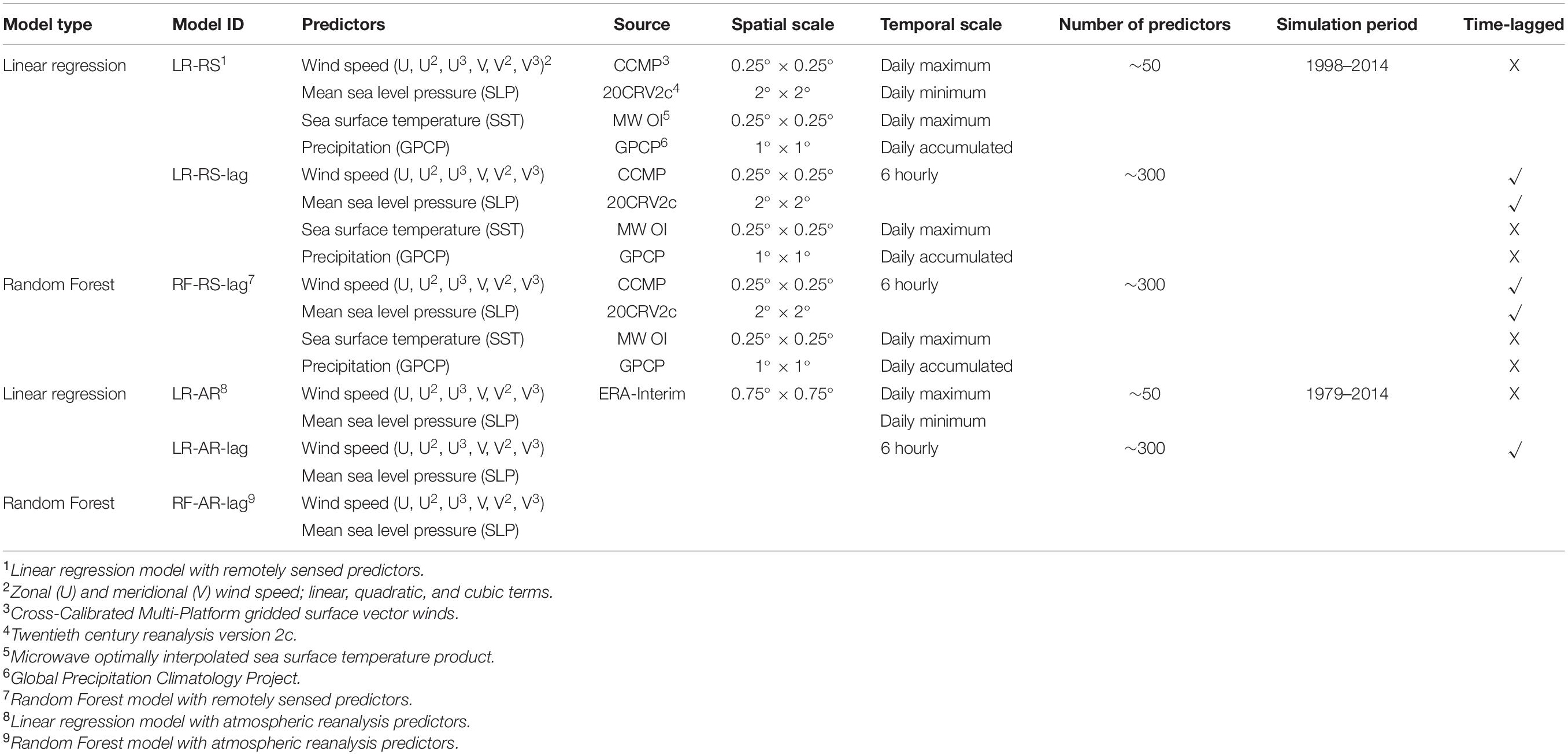
The data for this study come from several sources. Oceanographic and meteorological predictors used for the first objective are obtained from remotely sensed satellite products, where available. Table 1 outlines the different data and their respective temporal and spatial resolutions. 10 m wind speed from 1987 onward is acquired from the Cross-Calibrated Multi-Platform (CCMP) wind vector analysis product with a spatial resolution of 0.25 × 0.25 degrees and a temporal resolution of 6 h (Atlas et al., 2011). Daily global sea surface temperature (SST) from 1998 onward with a 0.25 × 0.25 degree spatial resolution is obtained from the microwave optimally interpolated SST product. Daily global precipitation from 1996 to 2015 with a 1 × 1 degree spatial resolution is acquired from the Global Precipitation Climatology Product (GPCP) (Huffman and Adler, 2001). SLP from 1871 to 2014 with 6 hourly temporal and 1 × 1 degree spatial resolution is obtained from the 20CRV2c (Poli et al., 2016). This predictor is obtained from a climate reanalysis since there is no global remote sensing product available for SLP. Furthermore, Cid et al. (2017) showed that the minimum SLP values during storms are more noticeable in 20CR than in ERA-Interim. For the second and third objective, 10 m wind speed and SLP data with a spatial resolution of 0.75 × 0.75 degrees and 6 hourly temporal resolution from the ERA-Interim reanalysis (Dee et al., 2011) are used as predictors.

TABLE 1

Table 1. Description of implemented data-driven models.

Predictands

Daily maximum surge is used as the predictand and derived from two different data sets. Observed sea level data for individual tide gages is obtained from the Global Extreme Sea Level Analysis (GESLA-2) database (Woodworth et al., 2017) and used to extract the daily maximum surge values (see section “Methodology”). The spatial distribution of the tide gages and available years of data during the 1979–2014 period are shown in Figure 1. In addition to in situ data, daily maximum surge values for the global coastline are obtained from GTSR (Muis et al., 2016). The data set (covering the period 1979–2014) is a near-coast global reanalysis of storm surges. It is obtained by forcing a hydrodynamic model, the Global Tide and Surge Model (GTSM) based on the Delft3D modeling suite, with wind speed and atmospheric pressure from the ERA-Interim reanalysis. Model outputs are provided in 16,395 locations along the global coastline. In order to compare the performance of the data-driven models with the hydrodynamic model, the closest GTSR grid points (out of the 16,395 locations) for each tide gage are identified and daily maximum surge values at those specific grid points are extracted. These values are then compared with daily maximum surge derived from the data-driven models and observed daily maximum surge.

FIGURE 1

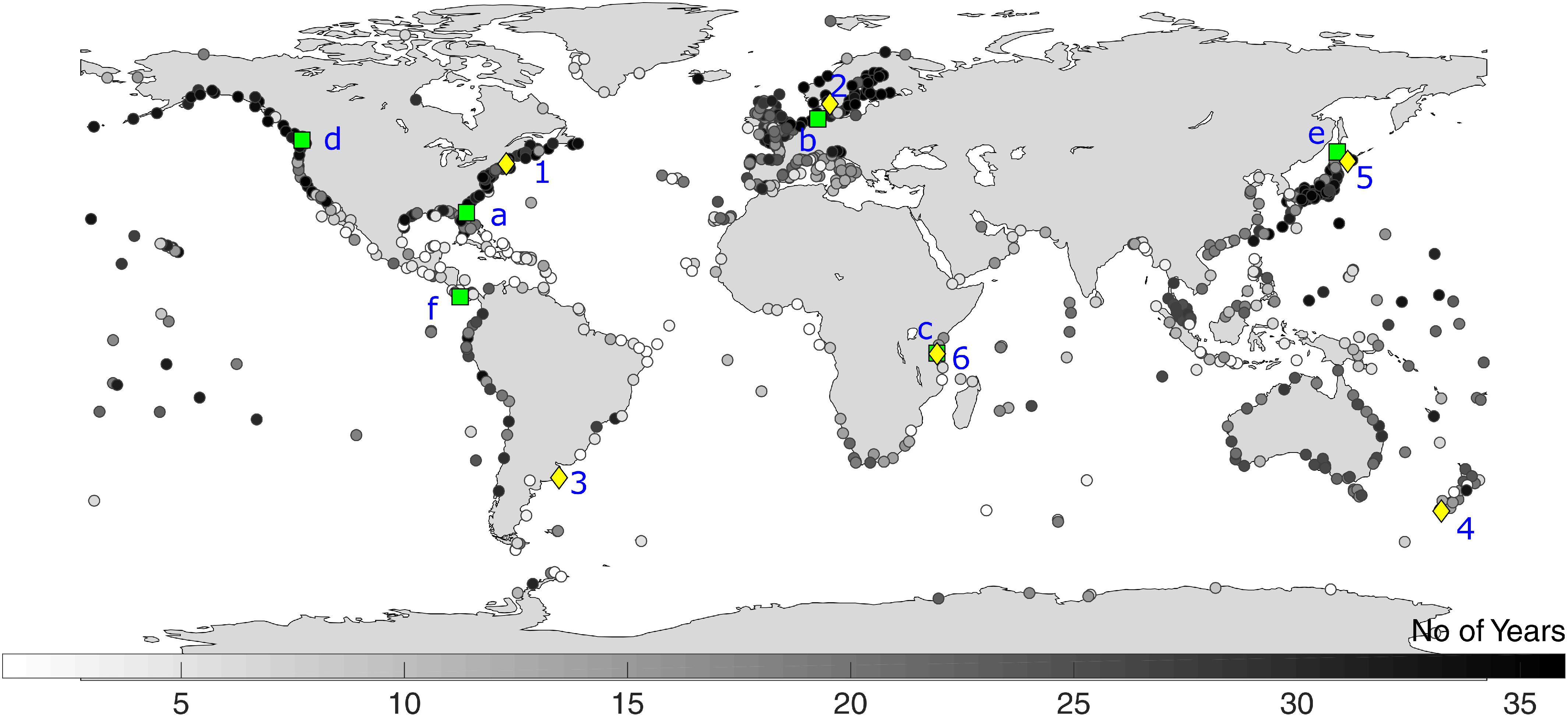
Figure 1. Number of years available for analysis during the 1979–2014 period. Green squares and yellow diamonds represent two sets of tide gages used in section “Results” to assess model performance in more detail: (a) St. Augustine, (b) Cuxhaven, (c, 6) Zanzibar (d) Victoria Harbor, (e) Wakkanai (f), Puerto Armuelles, (1) Boston, (2) Goteborg-Torshamnen, (3) Mar del Plata, (4) Bluff Harbor, and (5) Kushiro.

Methodology

Harmonic Analysis

Hourly sea level time series from the tide gages are de-trended by removing the annual mean sea level (Figure 2). Following this, the T_Tide Matlab package (Pawlowicz et al., 2002) is used to perform a classical harmonic analysis with 67 tidal constituents on a year-by-year basis. Predicted astronomical tides are subtracted from the de-trended sea level time series to separate non-tidal residuals. The UTide (Unified Tidal Analysis and Prediction Functions) (Codiga, 2011) package has also been tested with negligible differences in the results. Non-tidal residuals, considered in this study as storm surges, are used as predictands when developing and implementing the statistical and machine learning techniques outlined below. In some instances erroneous spikes were detected (and removed) from the storm surge time series, resulting from phase shifts between the predicted tide and observed water levels (see also section “Directions for Future Research”). The effects of waves are not included in the analysis.

FIGURE 2

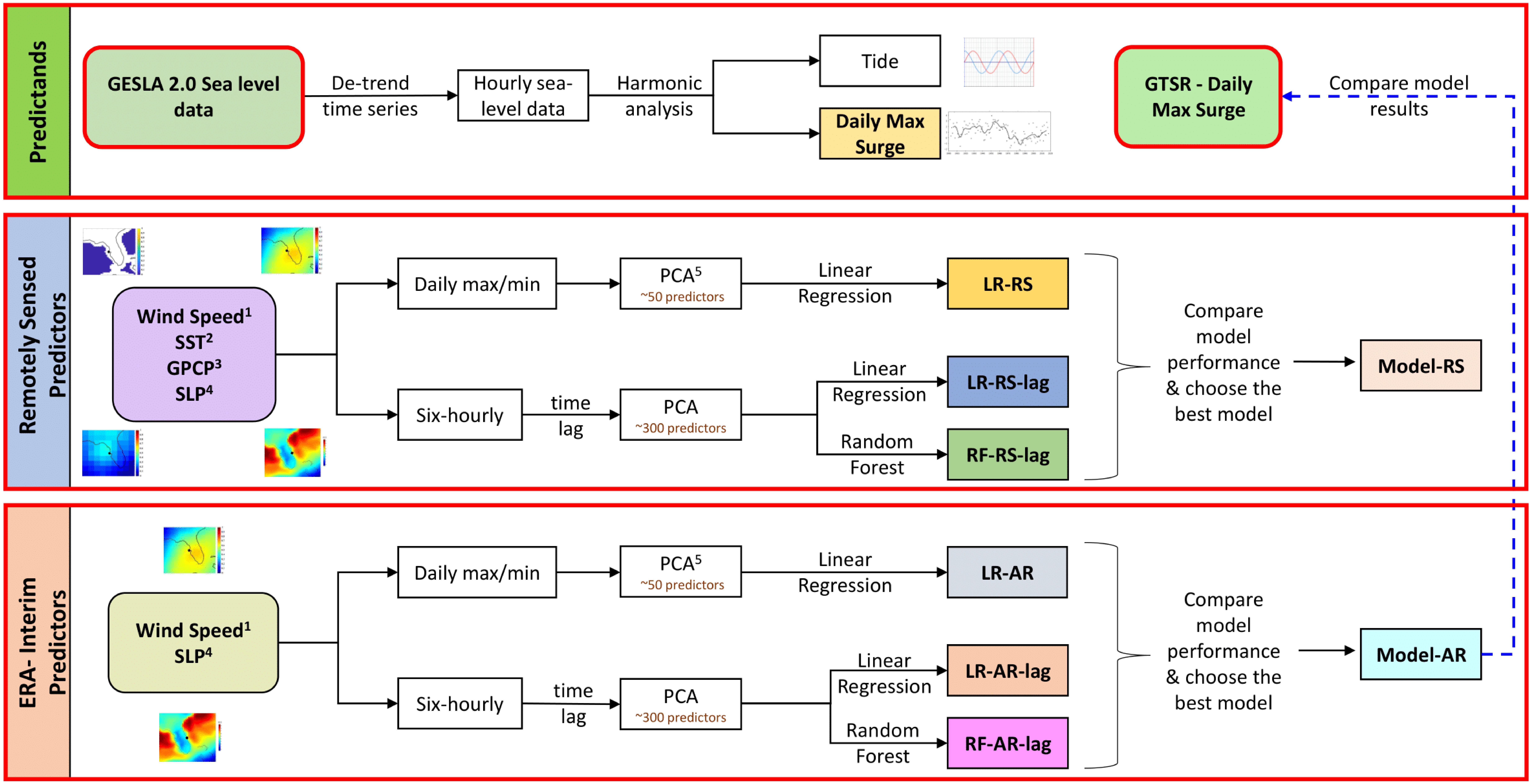
Figure 2. Framework outlining the applied methodology to develop data driven storm surge models using different predictor data sets, and comparison with numerical model output. Key: wind speed1, zonal and meridional wind speed; SST2, sea surface temperature; GPCP3, Global Precipitation Climatology Project; SLP4, mean sea-level pressure; PCA5, principal component analysis.

Predictor Selection

After identifying the daily maximum surge values for each tide gage, we localize meteorological and oceanographic predictors around each tide gage. Predictors within a 10 × 10 degree grid around the tide gages are considered for the analysis. In order to reduce the complexity of the models and the multicollinearity of predictor features, principal component analysis (PCA) is implemented (as in Cid et al., 2017, 2018). PCA is a multivariate analysis technique that reduces the dimensionality of a data set comprised of interrelated variables, while preserving the largest possible fraction of variability (Jolliffe, 2002). PCA transforms the original data to a new set of variables commonly known as principal components (PCs), which are uncorrelated and are sorted by how much of the variance in the original dataset is explained by each PC. Data from every grid point within the 10 × 10 degrees region around each tide gage are considered as predictors. Hence, the total number of predictors can get as high as 5,000. In order to reduce the large dimension, the PCs that explain 90% of the variance in the original data are selected for further analysis. This reduces the number of predictors to about 300–500. We also tested using all PCs that explain 95% of the variance. This did not improve the model performance, but adds more predictors and hence (unnecessary) model complexity.

Model Fitting

The first technique we test is based on multiple linear regression and we follow a stepwise procedure where we iteratively add or remove PCs of the respective predictors, only retaining those that provide significant information (p < 0.05). This reduces the complexity of the model while giving the best result possible. The daily maximum surge at a specific tide gage is then computed with the following equation:

$\text{Surge}(t,d)=a+\sum _{i=1}^N\sum _{j=1}^M{b}_{ij}\times P{C}_{ij}(t,d)$

where Surge (t, d) is the maximum surge on day d at the t-th tide gage, PC_ij (t, d) represents the j-th PC of the i-th predictor on day d, whereas N and M represent the total number of predictors and their corresponding number of PCs, respectively. a and b_ij are coefficients obtained from the regression model.

The second technique we implement and test is based on Random Forest, a supervised machine learning algorithm which incorporates the concepts of classification and regression trees, and bagging (where the model is trained using bootstrap samples of original predictor data) with some additional degree of randomization (see for example, Tyralis et al., 2019 for a detailed review of Random Forests). This study requires the implementation of Random Forest regression. The prediction of each trained regression tree is then averaged to provide a single value (here, the value of daily maximum surge at a tide gage location). Random Forests are (1) capable of capturing the non-linear dependencies between predictors and predictands, (2) fast and easy to use, (3) not prone to overfitting, and (4) suitable for high dimensional data (Tyralis et al., 2019). A sensitivity analysis is carried out to select the optimal number of regression trees for our analysis, based on the out-of-bag error, where the MSE for samples outside the bootstrapping set is quantified and minimized. For each tide gage, the out-of-bag error is computed for several numbers of bagged trees (1–200). This error is then normalized in order to compare results across tide gages (Figure 3). Considering the out-of-bag error behavior and the increased computational expense with an increased number of trees, we chose 50 as the optimal number for our analysis; beyond that the reduction in error is small, while the computational expense increases.

FIGURE 3

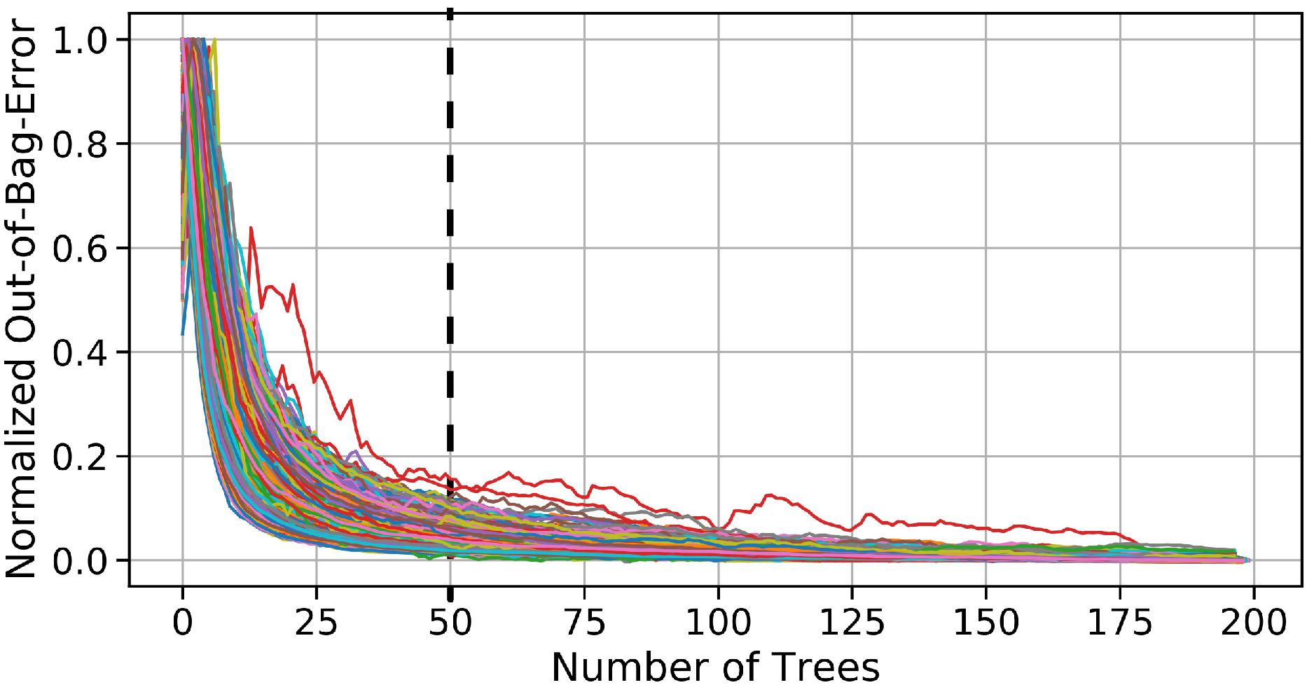
Figure 3. Sensitivity analysis to find the optimal number of decision trees: the relationship between the number of decision trees and the standardized out-of-bag-error. Each line represents the decrement of the standardized-out-of-bag-error of a tide gage with increase in the number of trees.

Model Configuration

Six different model configurations (see Table 1) are set up by varying the inputs (predictor types, either remotely sensed or atmospheric reanalysis) and their temporal resolution (daily and 6 hourly). Model IDs starting with LR represent model configurations that use linear regression to fit the model, whereas model IDs starting with RF represent model configurations that use Random Forest. Models trained with remotely sensed predictors have the suffix “RS” attached to the model ID. For instance, LR-RS is the model ID that represents models that use linear regression trained with remotely sensed predictors. On the other hand, the suffix “AR” is used to represent models trained with atmospheric reanalysis, particularly ERA-Interim reanalysis. For instance, RF-AR represents the Random Forest model trained with atmospheric reanalysis. We trained models with atmospheric reanalysis datasets for two reasons: the first one is to investigate the influence of the two types of predictors (from remote sensing and from reanalysis), on model accuracy. The second one is to compare the performance of the data-driven models with model outputs from GTSR, which is based on a hydrodynamic model and also uses ERA-Interim as forcing. As remotely sensed mean sea-level pressure is not available, models trained with remotely sensed predictors use mean sea-level pressure from 20CR. The period in which all the remotely sensed predictors overlap, and hence models are developed and tested, ranges from 1998 to 2014. Models trained with atmospheric reanalysis have a simulation period from 1979 to 2014.

In order to investigate the delay effects of predictors on daily maximum surge, predictors are lagged as far back as 30 h from the time the daily maximum surge occurred (i.e., predictors between the time of surge occurrence and 30 h before are all used in the regression models). For instance, LR-AR-lag represents the linear regression model that was trained with atmospheric reanalysis predictors that are lagged up to 30 h. Similarly, RF-RS-lag represents the Random Forest model trained with remotely sensed predictors that are lagged up to 30 h. Model IDs without the suffix “lag” represent models that are trained with predictors of daily temporal resolution. Hence, for each predictor type (remotely sensed and atmospheric reanalysis), there are three model configurations (see Table 1). Each of these three model configurations is evaluated by different performance metrics (see section “Model Validation”) and the model configuration that gives the highest performance metrics is chosen as the best model configuration for a given tide gage. For ease of interpretation, the collection of the best model configurations under the remotely sensed category is named as Model-RS. Similarly, the collection of the best model configurations under the atmospheric reanalysis category is named Model-AR.

Model Validation

Based on the data availability, we consider 732 tide gages for calibration/validation of Model-RS (using predictor information from remote sensing) and 840 tide gages for Model-AR (using predictor information from ERA-Interim). The models are validated using k-fold cross-validation. We follow Kohavi (1995) in selecting k = 10-folds. The validation process starts by randomly dividing the data set into k approximately equal groups, or folds. The model parameters are then estimated from using k−1 groups while the remaining group is used to test the model performance. Finally, the full time series can be reconstructed once all groups have been used for testing. We use the observed and reconstructed time series to compute three commonly used error statistics: Pearson’s correlation coefficient, Nash-Sutcliffe efficiency (NSE), and RMSE. One shortcoming inherent to the Pearson’s correlation coefficient (r) is that it only measures the strength of the relationship between the compared datasets, i.e., it does not indicate how similar the magnitudes of the compared time series are RMSE. On the other hand, quantifies the bias between the compared time series, but it is not a dimensionless metric. As a result, the modified Mielke index was proposed by Duveiller et al. (2016) as a combination of r and RMSE. We also derived this index (ranging from 0 for no agreement to 1 for perfect agreement) in addition to the three other metrics outlined above (results for the modified Mielke index are shown in the Supplementary Material).

We also test the sensitivity of the model results to the availability of tide gage data, by shortening the available tide gage records (until only one year of data is left for training and testing) and performing the same validation as outlined above.

Results

Model-RS – Models Forced With Remotely Sensed Predictors

This model category consists of three configurations, viz. LR-RS, LR-RS-lag, and RF-RS-lag (see Table 1). All three are trained and validated for 732 tide gages and results are compared with corresponding observed daily maximum surge values. For any given tide gage, the model configuration that gives the best error statistics in terms of Pearson’s correlation, RMSE, and NSE is selected for that specific tide gage (note that in all cases at least two of the error statistics pointed to the same best model configuration). In addition, the model was validated by the modified Mielke index and the results (very similar to the Pearson’s correlation coefficient) are shown in Supplementary Figure 1. On average, across all tide gages, we find that models LR-RS-lag and RF-RS-lag perform better than LR-RS (Figure 4; the same results but for tropical and extra-tropical regions separately are shown in Supplementary Figure 2); they are also selected at many more sites than LR-RS (Figure 5). LR-RS, which is forced with predictors of daily temporal resolution, gives the best eror statistics (highest correlation coefficient, highest NSE, and lowest RMSE) for only 12% of the tide gages (shown by diamonds in Figure 5A). The average correlation coefficient and RMSE are 0.64 and 7.8 cm, respectively. LR-RS-lag, which is forced with lagged predictors with 6 hourly temporal resolution, gives the best error statistics for most of the tide gages, 58% in total. The average correlation coefficient is 0.78 and average RMSE is 7.3 cm. This model configuration is effective mostly in subtropical/extratropical regions (shown by squares in Figure 5A; see also Supplementary Figure 8 for model performance across different latitude bands). RF-RS-lag gives the best error statistics for tide gages around the tropical region (the remainder 30% of sites, shown by circles in Figure 5A) with an average correlation coefficient of 0.5 and average RMSE of 5.7 cm. Higher correlation coefficients (as high as 0.9) are found in extratropical regions (30–60° north and south of the equator), whereas the tropical and sub-tropical regions (0–30° north and south of the equator) show lower correlation, especially along the west and north coasts of South America. The average correlation coefficient in the extratropical regions is 0.79, whereas in the tropical regions it drops to 0.45. The average RMSE in the extratropical regions is 7.5 cm, and 5.3 cm in tropical regions. These results match the ones that are reported by Cid et al. (2017), where average correlation in the extratropical and tropical regions are in the order of 0.8 and 0.5, respectively. In addition, Figure 5C displays the relative RMSE, which is the ratio of RMSE to the maximum surge variability at each tide gage (difference between highest and smallest daily maximum surge). In tropical regions, the relative RMSE is higher (up to 18%) compared to the extratropical regions. This value is also comparable with the one reported by Cid et al. (2017), which is 20%.

FIGURE 4

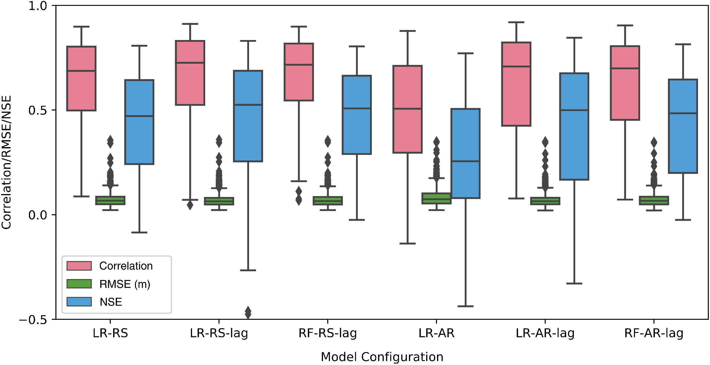
Figure 4. Validation of the six model configurations (LR-RS, LR-RS-lag, RF-RS-lag, LR-AR, LR-AR-lag, and RF-AR-lag) in terms of correlation coefficient, RMSE, and NSE.

FIGURE 5

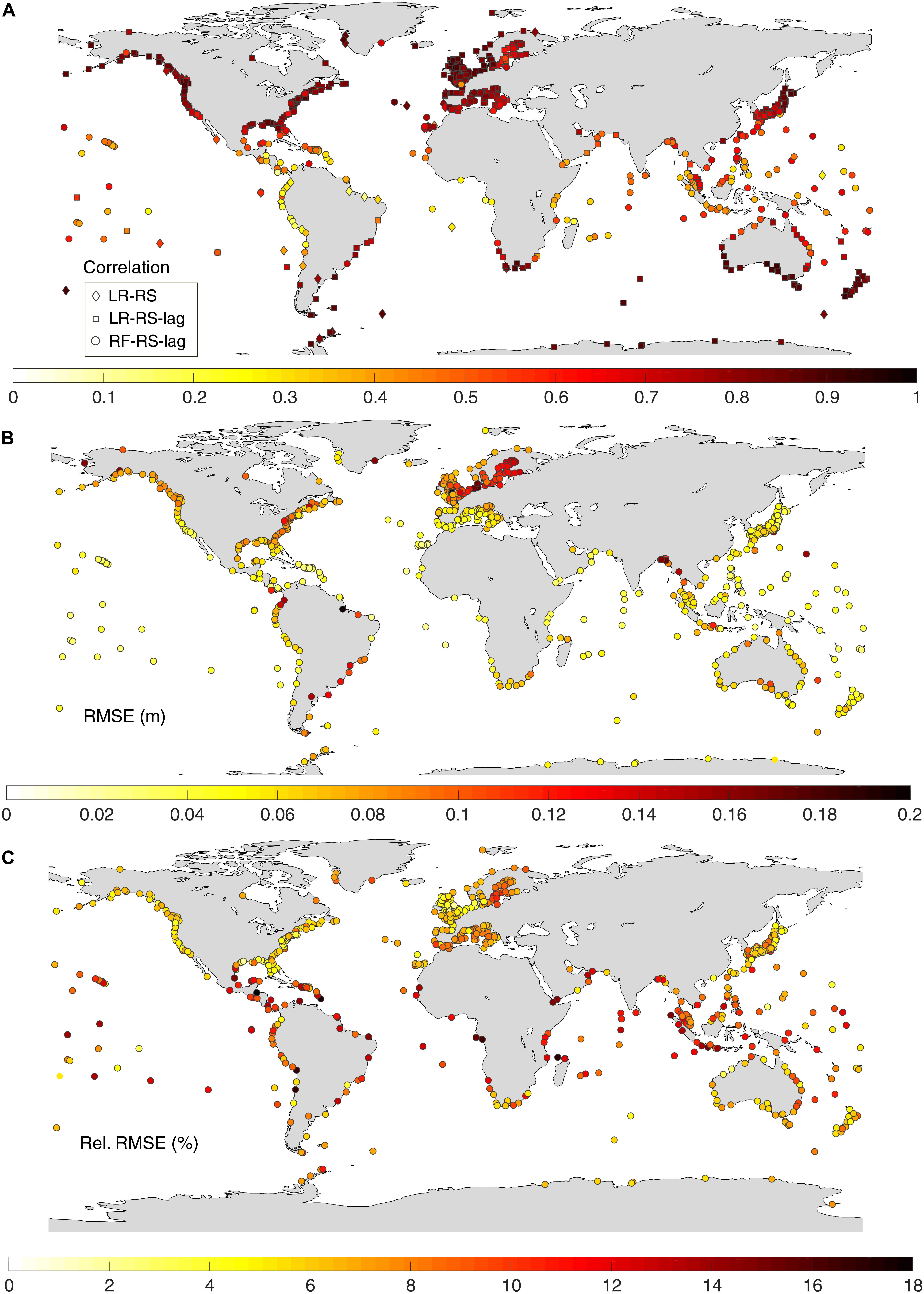
Figure 5. Validation of Model RS in terms of (A) Pearson’s correlation coefficient – diamonds, rectangles, and squares represent the three model configurations (LR-RS, LR-RS-lag, and RF-RS-lag) that make up Model-RS; (B) RMSE in m; and (C) relative RMSE in %.

Model accuracy of LR-RS is lower than that of LR-RS-lag and RF-RS-lag as it is relating daily min/max values of predictors with daily maximum surge. However, the daily maximum surge on a given day may also be affected by oceanographic and atmospheric conditions from previous days. The lower model accuracy for the tropical regions could be due to several reasons. First, historical time series analysis of the predictors shows that the variance of the most important predictors, wind speed and SLP, in tropical/sub-tropical regions are very low compared to extratropical regions (Supplementary Figure 3). Second, for some tide gages in the tropics (e.g., Santana, Brazil), river discharge may affect the tide gage measurements, adding additional non-tidal residuals that cannot be explained by the local predictors (the same mechanism would have a smaller effect in higher latitudes, where storm surges are relatively higher); rainfall may serve as a proxy to capture some of the discharge, but not when it is remotely driven (e.g., rainfall further upstream, or discharge from snow melt). Third, the predictors that explain tropical cyclone induced surges (for instance at the Bay of Bengal) are not captured well due to low temporal and spatial resolution.

Additional validation of Model-RS is shown in Figure 6. Six tide gages (marked as green squares in Figure 1), are chosen from different climatic regions to assess model performance for a specific year (2007) by comparing observed and simulated daily maximum surge time series (Figure 6, left), scatter plots (Figure 6, middle), and quantile–quantile plots (Figure 6, right). For tide gages in sub-tropical and extratropical regions (St. Augustine, Cuxhaven, Victoria Harbor, and Wakkanai), the daily maximum surge is relatively well reproduced with minimum and maximum correlation of 0.79 and 0.91, respectively; in some cases lowest surges are overestimated and highest surges are slightly underestimated. However, for tide gages in tropical regions (Zanzibar and Puerto Armuelles), the daily maximum surge is strongly underestimated.

FIGURE 6

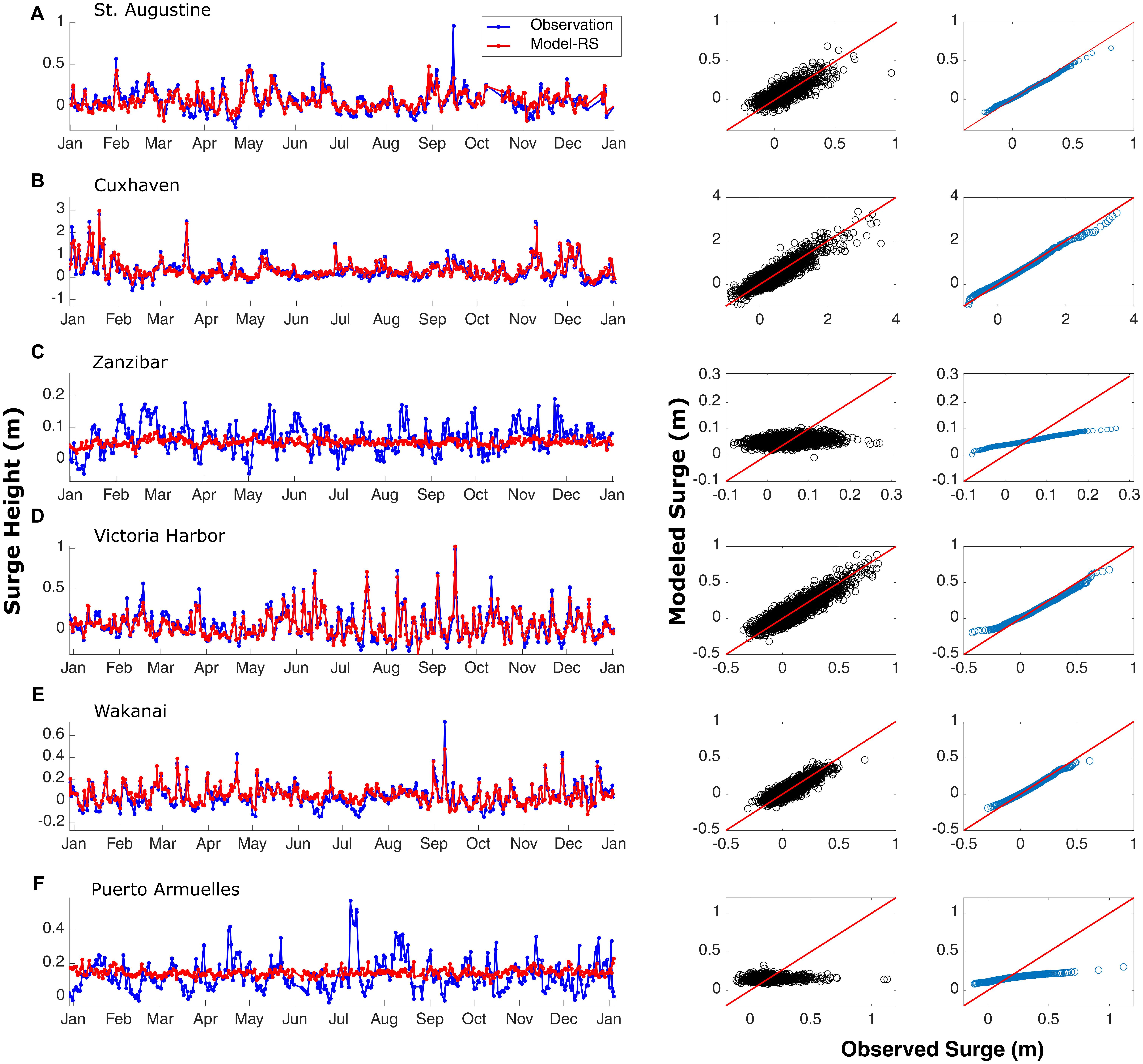
Figure 6. Daily maximum surge time series comparison (left), scatter plots (middle), and quantile-quantile plots (right) for observed and modeled (Model-RS) daily maximum surge for six tide gage locations (marked in green in Figure 1).

Figure 7 displays the performance of Model-RS in capturing extreme surge events. Observed surge values above the 95th percentile threshold of the daily maximum surge are selected for the same tide gages shown in Figure 6, and compared to corresponding surges derived from Model-RS. Again, model performance increases from low to high latitudes. Extreme surge events are better reproduced at Cuxhaven (r = 0.78), Victoria Harbor (r = 0.75), and Wakkanai (r = 0.61), compared to Zanzibar (r = −0.11) and Puerto Armuelles (r = −0.04) in the tropics, where the model strongly underestimates the extreme surge events (all modeled surge values are below the 1:1 reference line). Validation of Model-RS for extreme surges globally (Supplementary Figure 7) leads to an average correlation of 0.54 and an average RMSE of 14.5 cm in extratropical regions, whereas in the tropics the average correlation is 0.32 and average RMSE is 13.1 cm.

FIGURE 7

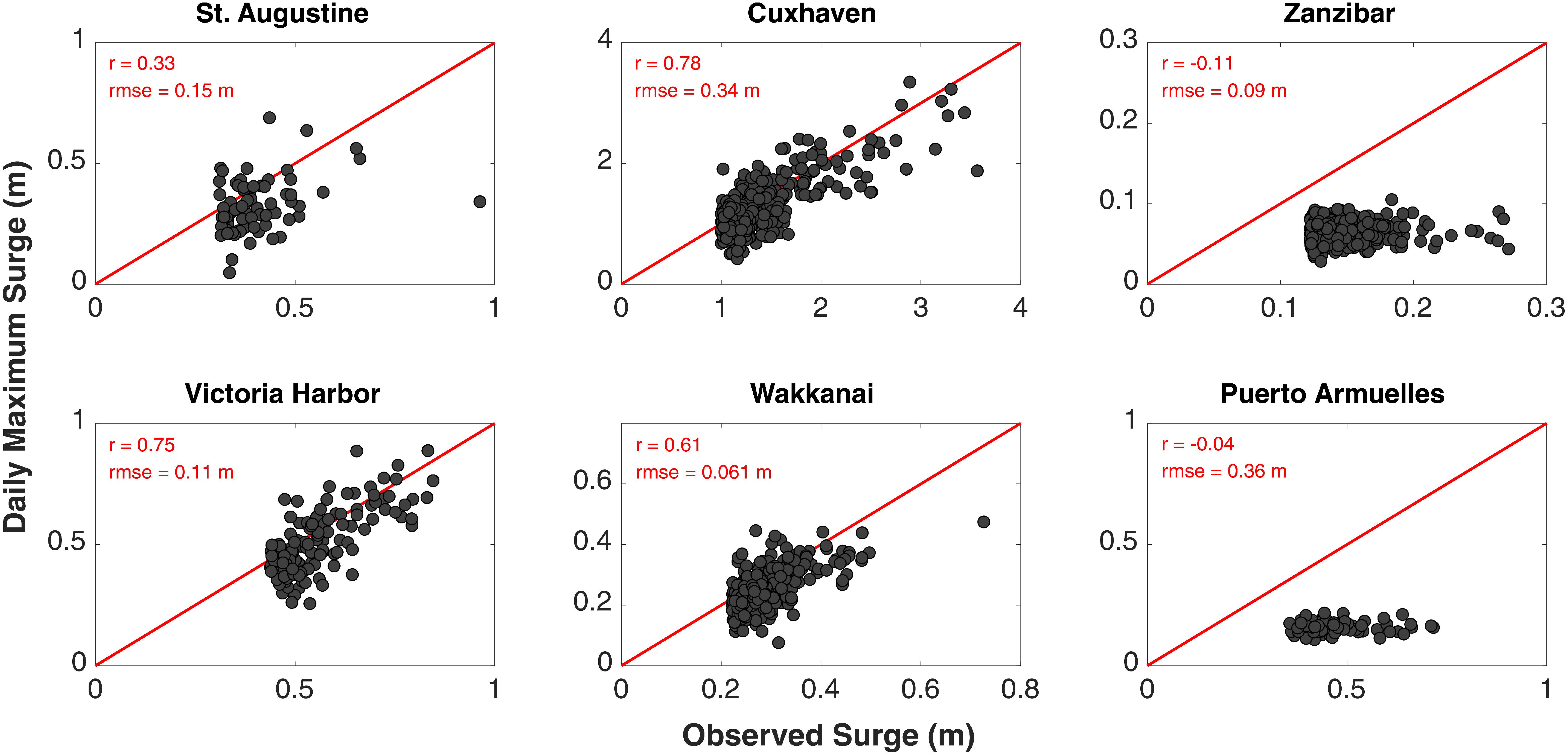
Figure 7. Validation of Model-RS performance for extreme events (surge values above the 95th percentile threshold).

Finally, extreme total still water levels (here, defined as events above the 95th percentile threshold) are calculated by superimposing the corresponding daily maximum surge and tide values for each tide gage. The observed and modeled total still water levels have very strong agreement at the vast majority of the tide gages [Figures 8 and Supplementary Figure 8 (right)]; the average correlation coefficient is 0.74 and average RMSE is 9.4 cm. This overall improvement is to be expected, as the tidal component is the same in both the observed and modeled datasets. Tide gages in the Gulf of Mexico, the Mediterranean Sea, and the Baltic Sea have slightly lower correlation. The total still water level (at the time of daily maximum surge) at these locations is dominated by the surge while tidal contributions are small, or even negligible. Surges at these locations are, however, also simulated with relatively lower accuracy compared to other locations (Figure 5C), which in turn propagates to the total still water level results presented here.

FIGURE 8

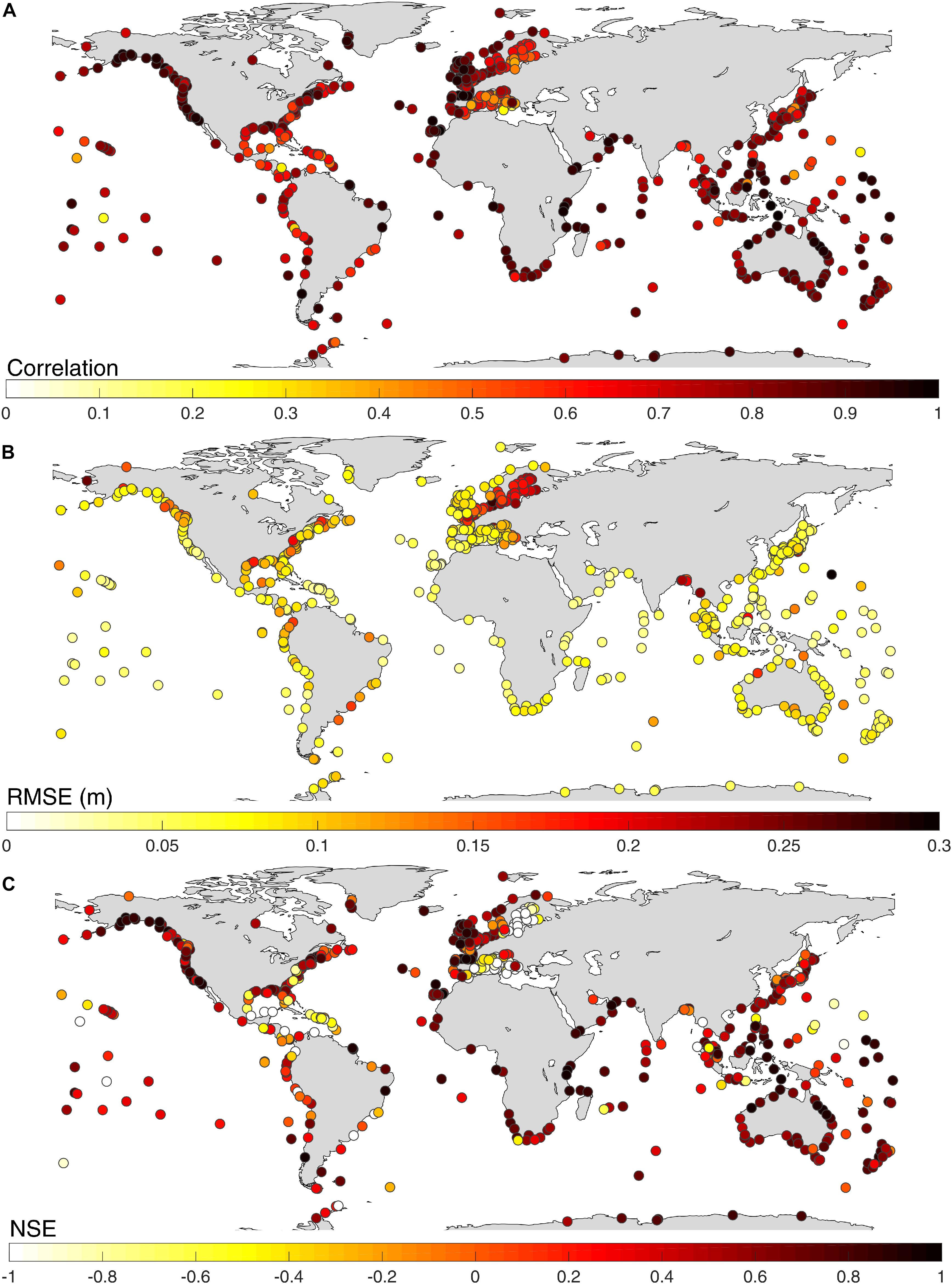
Figure 8. Validation of Model-RS for total still water levels above the 95th percentile threshold: (A) Pearson’s correlation coefficient; (B) RMSE in m; and (C) NSE.

The relative importance of predictors in Model-RS is also investigated. Since two model fitting techniques are used (linear regression and Random Forest), the predictor importance is assessed for both methods separately. For the linear regression method, important predictors would have relatively higher regression coefficients. The level of importance of all predictors across all tide gages according to the linear regression and Random Forest models are shown in Figure 9. For the Random Forest method (pertaining to RF-RS-lag), the values of each predictor are randomly reordered (permuted) and the change in the accuracy of Model-RS is measured in terms of MSE. A predictor that, when randomly reordered, affects the accuracy of RF-RS-lag significantly is considered an important predictor. Therefore, predictors in Figure 9 are ranked based on how much they can modify results of Model-RS. For linear regression, it is found that mean sea-level pressure is the most important predictor for 77% of the tide gages, followed by daily accumulated precipitation (16%), and meridional wind speed (3%). Whereas the Random Forest analysis shows that mean sea-level pressure is the most important predictor for about 65% of the tide gages, followed by meridional wind speed (12%), and SST (10%). Overall, both models (linear regression and Random Forest) point to mean sea-level pressure and its time-lagged components as the most important predictors to model daily maximum surge at the majority of the tide gages.

FIGURE 9

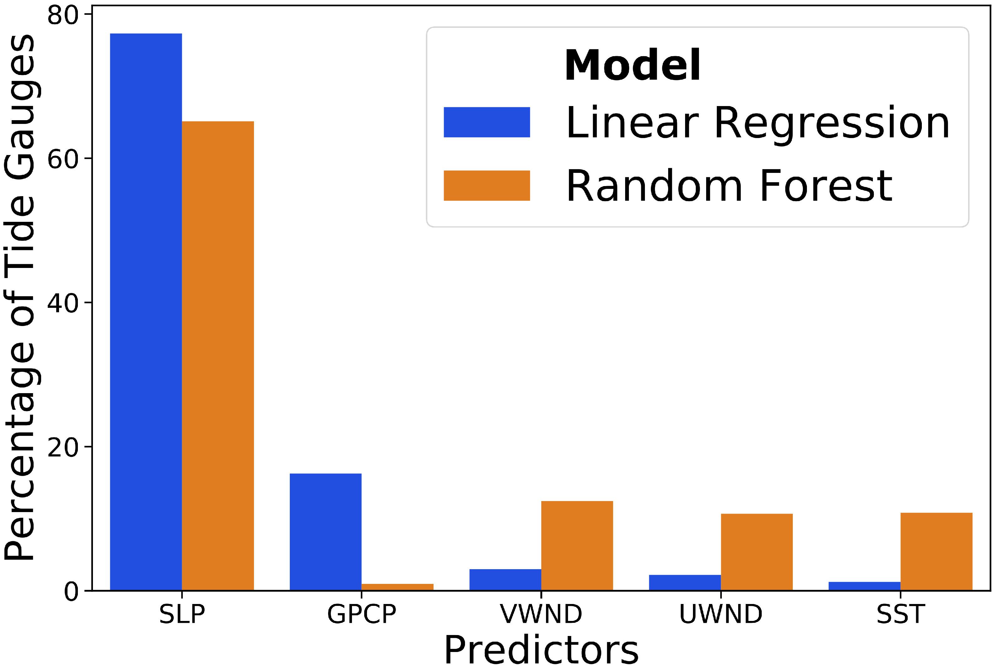
Figure 9. Percentage of the number of tide gages where individual predictors are deemed most relevant (see text for more details) for Model-RS for stepwise regression and Random Forest; VWND and UWND are zonal and meridional wind speeds.

Model-AR – Models Forced With Predictors From ERA-Interim Reanalysis

Under this category, three model configurations (LR-AR, LR-AR-lag, and RF-AR-lag) are forced with wind speed and SLP from the ERA-Interim reanalysis. This is done for two main purposes: (1) to investigate the added value (if any) of using remotely sensed predictors, (as in Model-RS) as compared to atmospheric reanalysis data, and (2) to compare the performance of the data-driven model with GTSR. Model configurations under this category, LR-AR, LR-AR-lag, and RF-AR-lag give the best error statistics for 4, 62, and 34% of the tide gages, respectively. Average correlation coefficients for the three model configurations are 0.39, 0.77, and 0.46, whereas average RMSE values are 7.7, 7.6, and 5.6 cm, respectively. As in the case of Model-RS, LR-AR-lag gives the best results for tide gages in the sub-tropical/extratropical regions. Figure 10 displays the validation of Model-AR in terms of Pearson’s correlation coefficient, RMSE, and relative RMSE. Further validation results pertaining to Model-AR are shown in Supplementary Figures 4–6. Similar to Model-RS, the daily maximum surge from these model configurations shows strong agreement with observed daily maximum surge in the sub-tropical/extratropical regions, where the average correlation coefficient is 0.75. This value drops to 0.42 in the tropical regions for the same reasons explained in section “Model-RS – Models Forced With Remotely Sensed Predictors”. Average RMSE is 7.8 and 5.5 cm in the sub-tropical/extratropical and tropical regions, respectively. The highest relative RMSE is found in the tropics (reaching up to 18% of the daily maximum surge variability). LR-RS performs better in all three performance statistics compared to LR-AR (see Figure 4). In addition, LR-RS-lag and RF-RS-lag are also performing slightly better than LR-AR-lag and RF-AR-lag. When choosing the best model configuration for Model-RS and Model-AR the mean correlation coefficients are 0.68 and 0.65, respectively, whereas the mean RMSE values are 6.9 and 7 cm. It has to be noted that the spatial resolution of the wind speed used for Model-RS is three times higher than that of the reanalysis wind speed (see Table 1). However, the spatial resolution of the SLP in Model-RS (coming from 20CRV2c, as no remote sensing product is available) is approximately three times coarser than the one used for Model-AR.

FIGURE 10

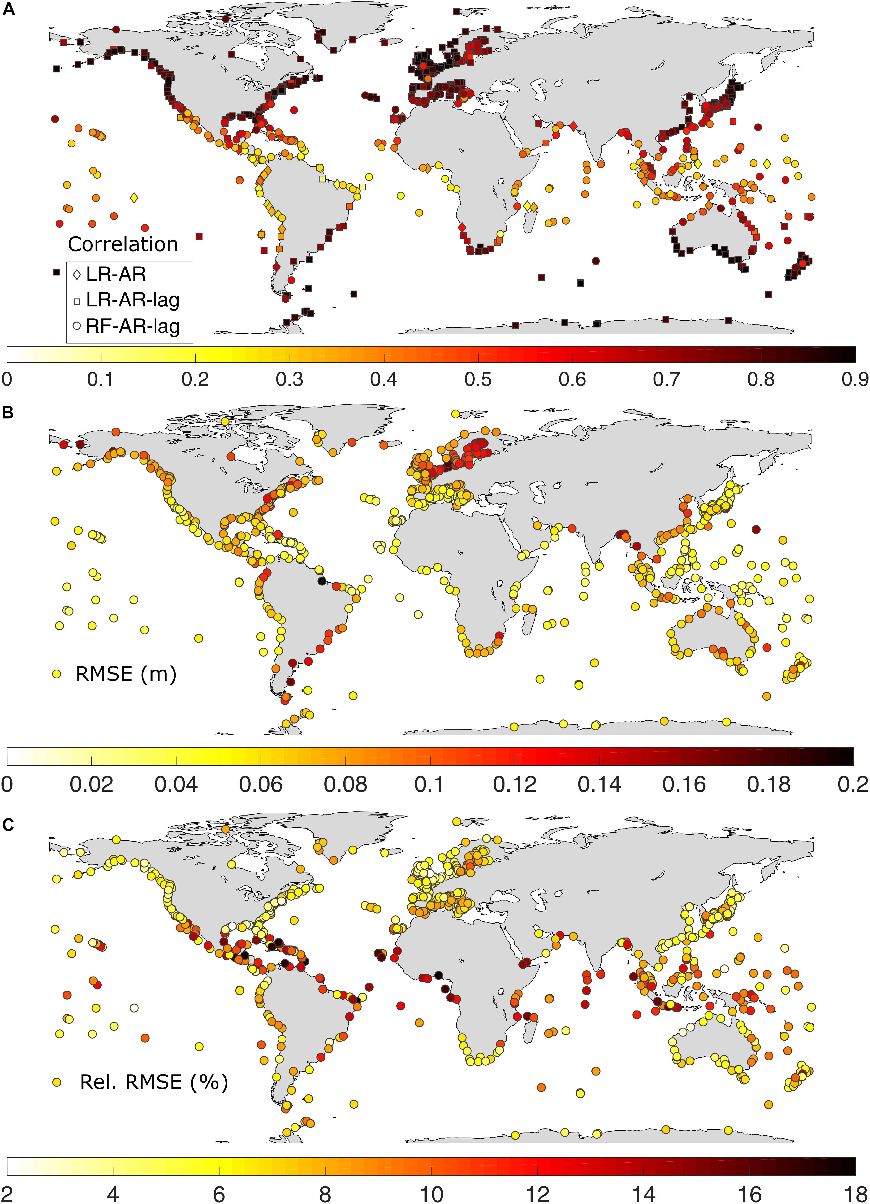
Figure 10. Validation of modeled (Model-AR) daily maximum surge in terms of (A) Pearson’s correlation coefficient – diamonds, rectangles, and squares represent the three sub-models (LR-AR, LR-AR-lag, and RF-AR-lag) that make up Model-AR; (B) RMSE in m; and (C) relative RMSE in %.

We also used this model setup to test the sensitivity of model accuracy with respect to data availability and found that as little as 5 years of data is required to achieve good model accuracy and further increase in data availability does not improve model accuracy (see Supplementary Figure 9).

Comparison With GTSR

As described in section “Data”, the GTSR grid points closest to the tide gages are identified and the daily maximum surge time series at these grid points are extracted for the 1979–2014 period. The surge values from GTSR are then compared with observed values (for the overlapping periods) and are validated using Pearson’s correlation coefficient and RMSE. Average correlation and RMSE are 0.54 and 11.2 cm, respectively. For sub-tropical/extratropical regions, average correlation and RMSE are 0.65 and 11 cm, whereas for tropical regions average correlation and RMSE are 0.28 and 13 cm, respectively. The direct comparison of performance between Model-AR and GTSR (both forced with ERA Interim reanalysis data) is shown in Figure 11.

FIGURE 11

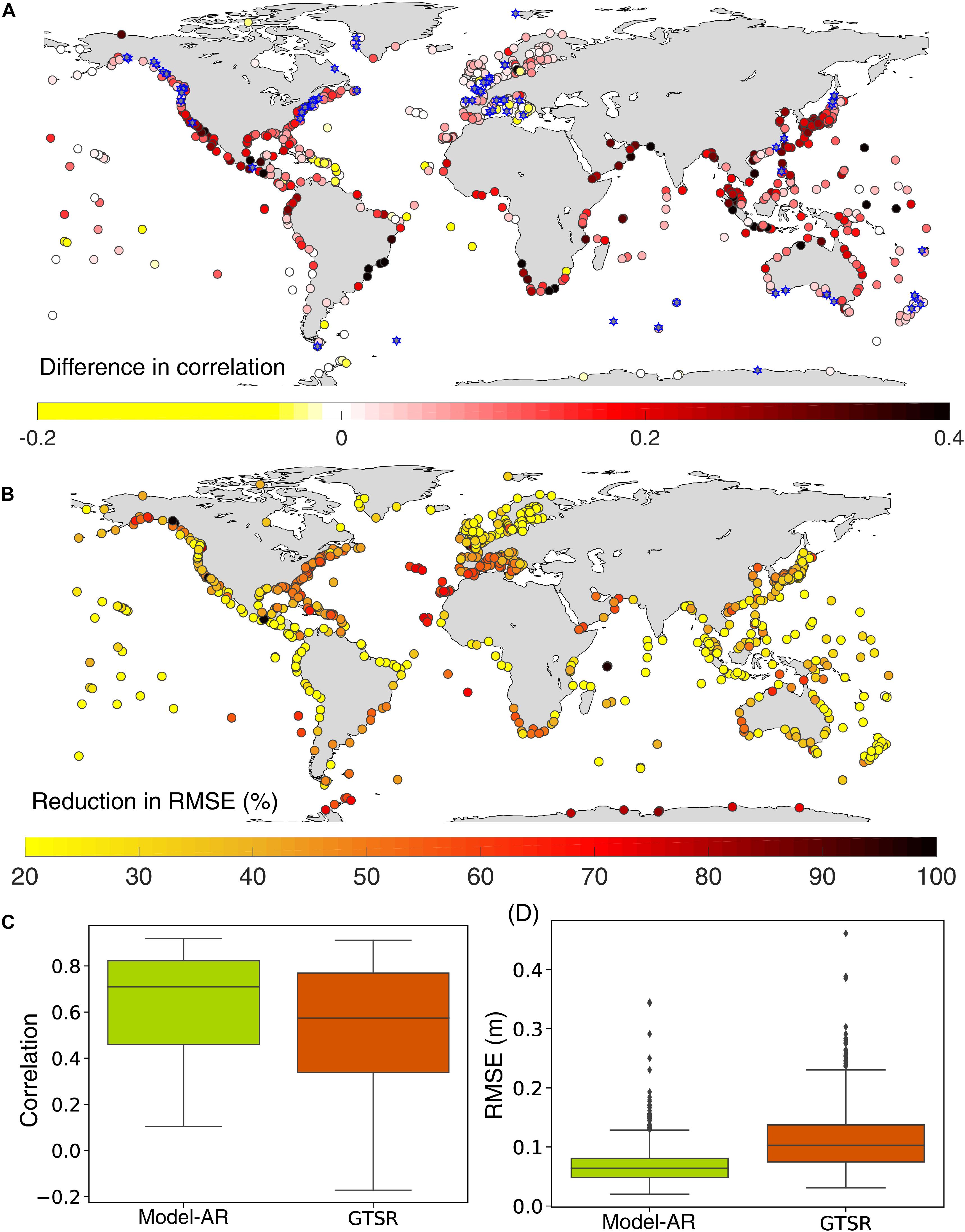
Figure 11. Comparison of Model-AR with GTSR. (A) Difference in Pearson’s correlation coefficients of Model-AR and GTSR with observations. Red colors indicate that Model-AR has higher correlation than GTSR, whereas blue stars denote tide gages where the difference in correlation is insignificant. (B) Reduction of RMSE in Model-AR compared to GTSR expressed in percent. Boxplot comparison of correlation (C) and RMSE (D) for Model-AR and GTSR.

Figure 11A displays the spatial differences in correlation between GTSR and Model-AR, i.e., comparing correlation coefficients for Model-AR vs observations and correlation coefficients for GTSR vs observations. The Fisher’s Z transformation method is used to assess significance of the difference between the two correlation coefficients. For a large percentage (92%) of the tide gages, there is a significant difference between the two correlation coefficients (Model-AR and GTSR have no significant difference in correlation for tide gages marked by blue stars in Figure 11A). and for 88% of these tide gages Model-AR has higher correlation coefficients than GTSR. Similarly, the RMSE for both models vs observations is computed and is found to be lower for Model-AR at all tide gages (Figure 11B).

Figure 12 illustrates a comparison of daily maximum surge time series and scatter plots from Model-AR, GTSR, and observations. Model results for six tide gages, which are also shown in Muis et al. (2016) and marked as yellow diamonds in Figure 1, are chosen for illustration. Both Model-AR and GTSR reproduce the observed surges well in locations such as Goteborg and Kushiro. However, Model-AR simulates the surge events better than GTSR at Mar del Plata (GTSR underestimates), Bluff Harbor (GTSR overestimates), and at many other tide gages not shown here. However, both models fail to simulate the daily maximum surge at Zanzibar, owing to very little variance of predictors that cannot explain the variation in the predictand. In order to test the performance of the two models for extreme events, observed surge values above the 95th percentile threshold are compared with their corresponding Model-AR and GTSR values in Figure 13, including scatter plots (left) and quantile–quantile plots (right). Differences in model performance for extreme events are most evident for Boston and Mar del Plata, where GTSR underestimates the surge values, and at Bluff Harbor, where GTSR overestimates the extreme surge values. Both models perform poorly for Zanzibar.

FIGURE 12

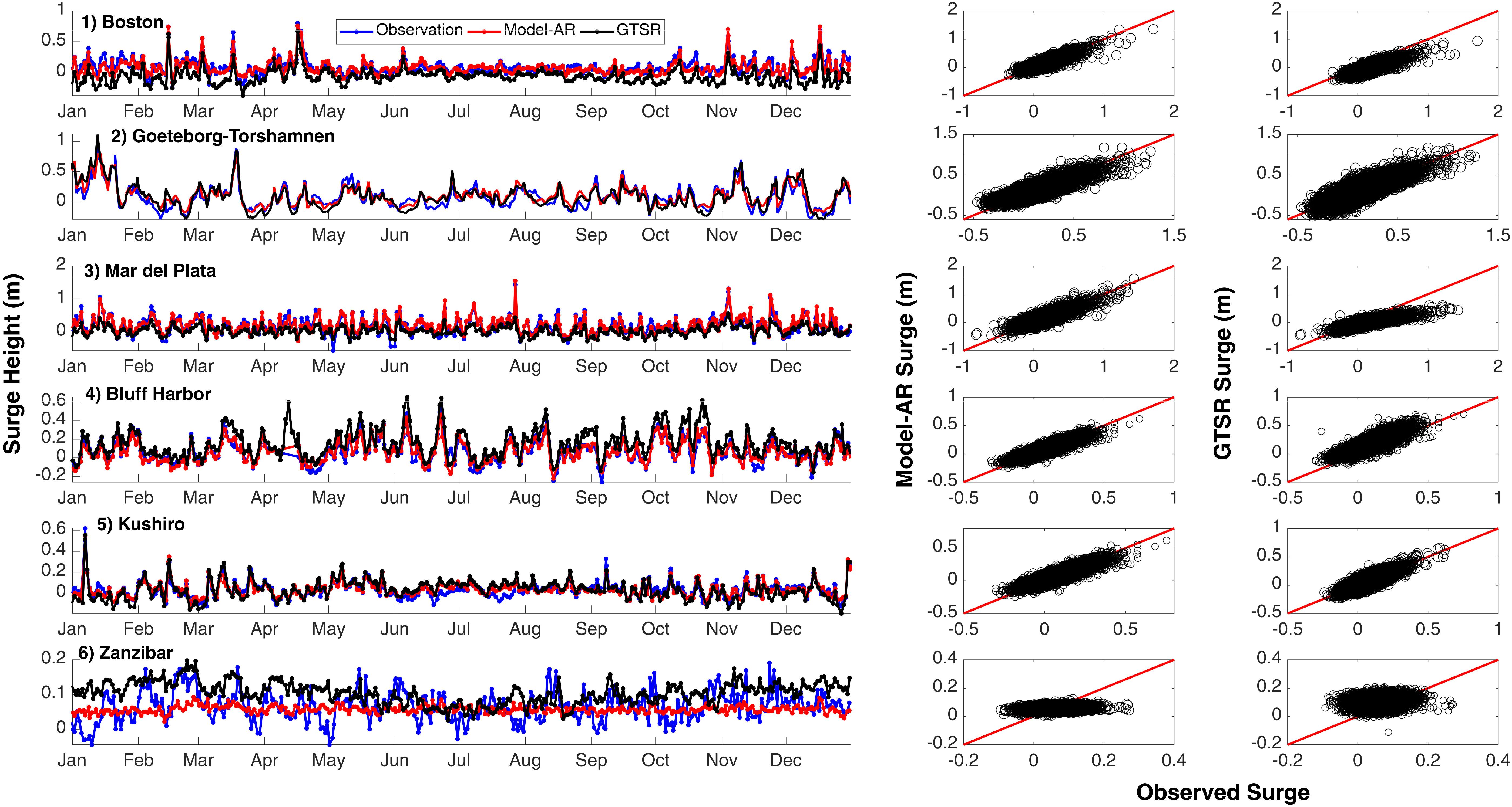
Figure 12. Daily maximum surge time series comparison between observations, Model-AR, and GTSR (left); scatter plots for Model-AR and observed surge values (middle) and scatter plots for GTSR and observed surge values (right) for tide gages marked in yellow in Figure 1.

FIGURE 13

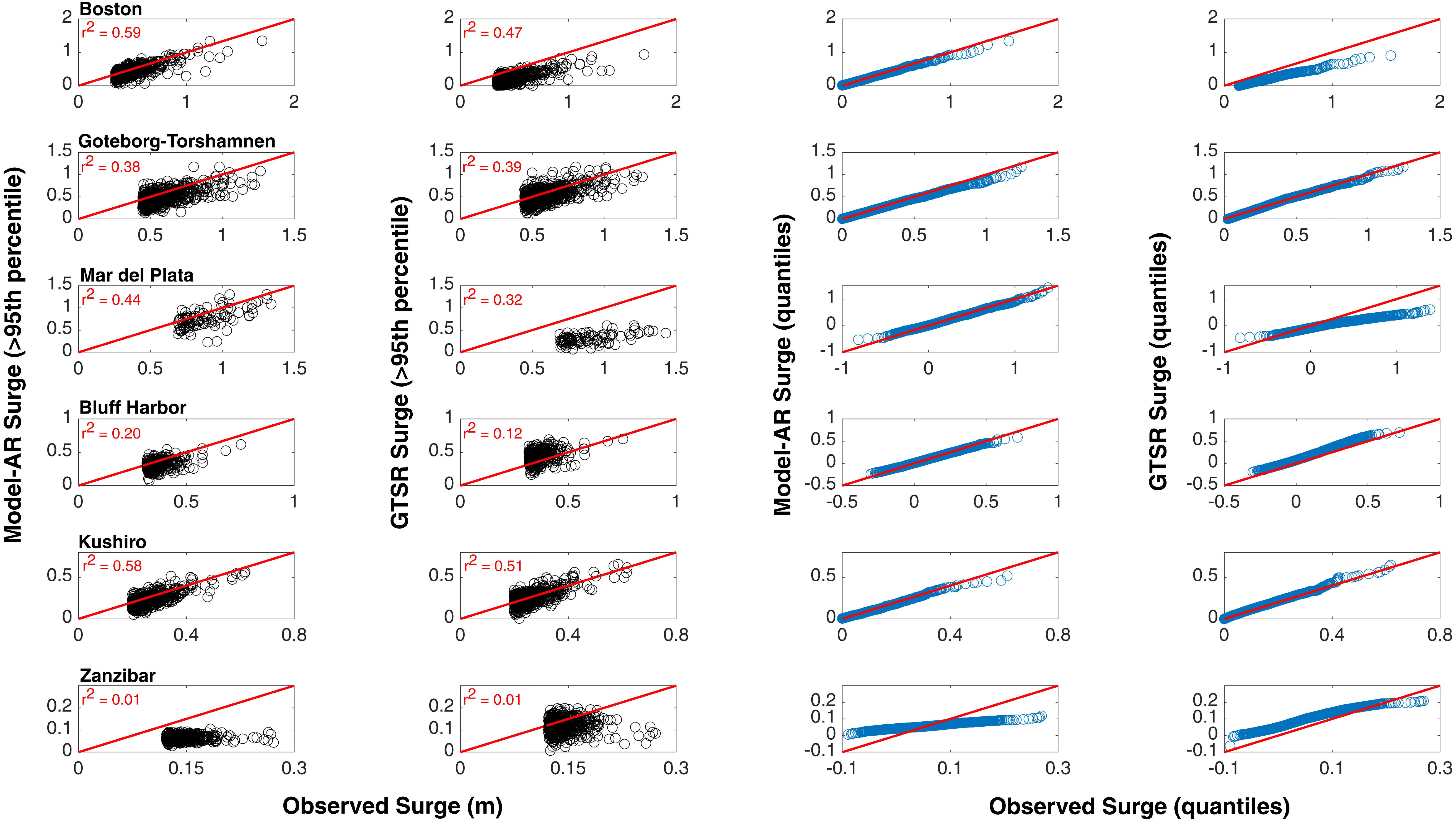
Figure 13. Performance of Model-AR and GTSR (see y-axis labels) for extreme surge events (surge values higher than 95th percentile of observed daily maximum surge) shown as scatterplots (left) and q–q plots (right).

Concerning extreme storm surges, Model-AR has an average correlation of 0.51 and 0.29 in extratropical and tropical regions, respectively. For GTSR correlation is lower, 0.44 and 0.20. Model-AR has an average RMSE of 15 and 13 cm in extratropical and tropical regions. For GTSR RMSE is higher, 23 and 19 cm. Model results are also validated for specific extreme events. Three tropical/extratropical events (Superstorm Sandy, Cyclone Xaver, and Hurricane Katrina) are selected to test the performance of the three models: Model-RS, Model-AR, and GTSR. Three tide gages are chosen for each event as shown in Figure 14. Model-RS and Model-AR show similar results for all cases, whereas GTSR often underestimates the peak surge, e.g., at Bridgeport during Superstorm Sandy, or for Hurricane Katrina at all three tide gages. The surge values during Cyclone Xaver are well captured by all models, except for a slight overestimation by Model-RS and GTSR.

FIGURE 14

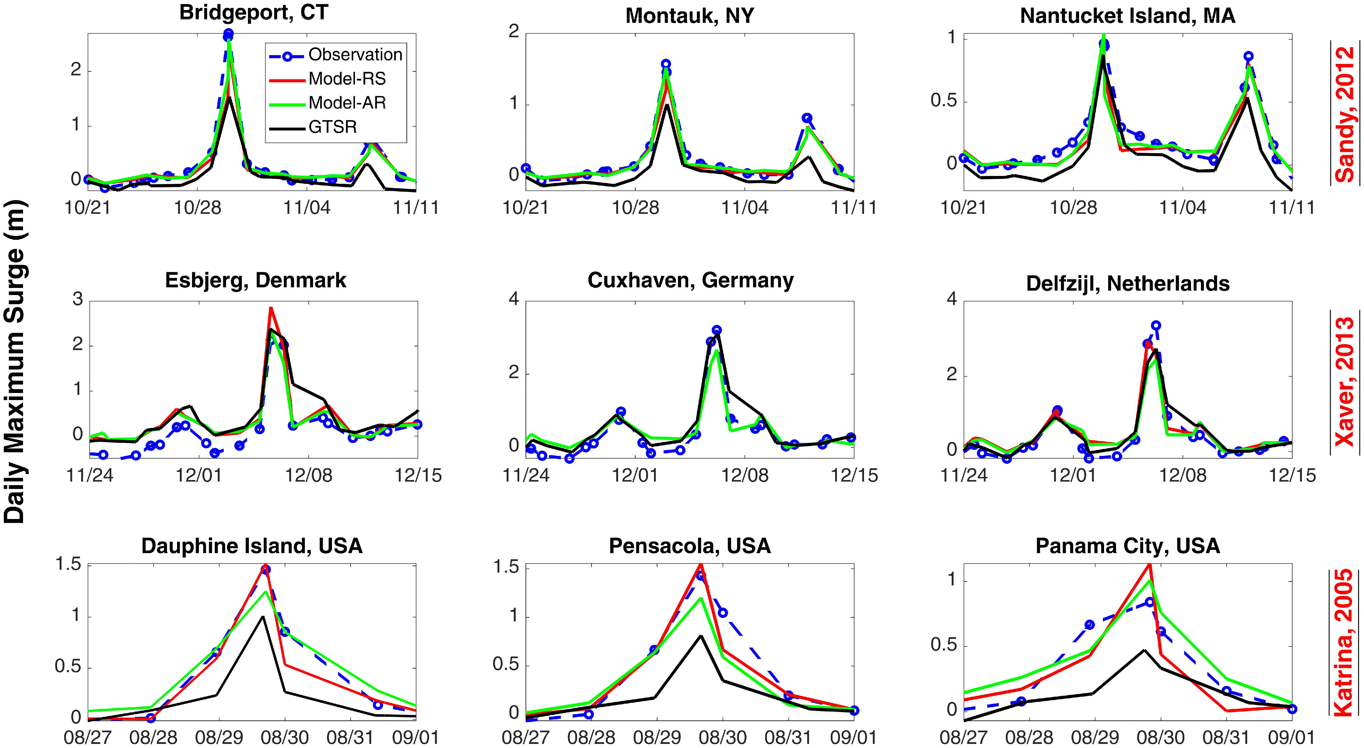
Figure 14. Validation of Model-RS, Model-AR, and GTSR for individual storm events: Superstorm Sandy (top), Cyclone Xaver (middle), and Hurricane Katrina (bottom).

Directions for Future Research

Although the data-driven models show better performance than the numerical model, a number of expansions (discussed below) could further improve the predictive skill.

The effects of wave set-up have not been incorporated in this study. However, Tait (1972) has shown that in tropical and sub-tropical islands, wave set-up can add more than 20% of the incident wave height to the “tide + surge” estimation of the sea level. Incorporating this effect (e.g., with simple approximations as in Vousdoukas et al., 2018) using data from models akin to the one used by Perez et al. (2017) and Camus et al. (2017) could potentially improve the model performance, especially in the tropics, where model accuracy of the data-driven models (but also GTSR) is poor.

Model accuracy would also likely increase when predictors with higher spatial and/or temporal resolution are used. Bloemendaal et al. (2019) showed that a horizontal resolution of 0.225° is adequate to simulate tropical cyclone induced storm surges. New reanalysis products such as ECMWF re-analysis Version 5 (ERA-5) (Hersbach et al., 2019) or The Modern-Era Retrospective-analysis for Research and Applications, Version 2 (MERRA-2) (Bosilovich et al., 2016) have recently become available and could be used to improve storm surge modeling in the tropics. Furthermore, the comparison between Models-RS and Model-AR would be more complete with the availability of remotely sensed global SLP data. We show that SLP is the most important predictor for modeling storm surges at many tide gage locations, and hence further analysis would allow for a better understanding of the value of remotely sensed and reanalysis predictors for data-driven (but also hydrodynamic) storm surge modeling.

In several recent studies authors opted to use skew surge, which is the absolute difference between the maximum observed sea level and the predicted tidal high water within a tidal cycle (Williams et al., 2016), as an alternative measure to non-tidal residuals (e.g., Haigh et al., 2015; Marcos and Woodworth, 2017). This has the advantage of reducing the amount of errors in the storm surge proxy when there are small phase shifts in the observations or tidal predictions; those can lead to artificial high peaks in non-tidal residuals, whereas skew surges are less affected by such errors. Skew surges are also largely independent of the phase of the tide, at least in regions where semi-diurnal tides dominate. Santamaria-Aguilar and Vafeidis (2018) showed that in mixed tidal regimes there is still dependence between extreme skew surge events and tides. A significant shortcoming of the skew surge concept consists in the loss of the hydrograph information, which is essential for inundation and risk assessments. Here, we use non-tidal residual data instead of skew surge for the global analysis, as this allows direct comparison with the results presented in earlier studies, such as GTSR. We tested using skew surge at selected sites and found very similar results compared to using non-tidal residuals in terms of model performance.

Another area of improvement would be to include tide-surge interaction in either the modeling of surges (or skew surges) or when combining the surge data with tidal data to obtain total still water levels. We use the same approach as Muis et al. (2016), which ignores tide-surge interaction, but allows a direct comparison of the results. Capturing tide-surge interaction in numerical model studies requires running coupled tide-surge simulations (Pugh and Woodworth, 2014), which increases the computational cost significantly.

The methodology presented here can be implemented operationally to provide daily maximum surge forecasts at tide gages around the globe. The data-driven models could be forced with forecast wind speed and SLP as well as other relevant predictors. Tidal predictions can be superimposed to the predicted surges in order to compute the forecast total still water level. In order to include uncertainty stemming from predictors (captured through ensemble forecasting systems), the modeling paradigm could shift from deterministic (implemented in this study) to probabilistic. Such a tool could possibly provide useful information for decision-makers, or inform other modeling efforts, in particular in regions where no dedicated storm surge forecasting systems are in place. Finally, surge values derived from GTSR can also be used as predictand (instead of surge values derived from tide gage observations) to train and validate data-driven models with full global coverage, including ungaged locations.

Conclusion

In this study, we explored the applicability of data-driven models to simulate global storm surges. Our first objective was to train and validate data-driven models (based on multiple regression and Random Forest) at tide gage locations across the globe for the purpose of simulating daily maximum surge; models were trained and validated at more than 800 tide gages. The predictand, daily maximum surge, is simulated well in sub-tropical and extratropical regions with average correlation coefficients of 0.79 and 0.75 for Model-RS and Model-AR, and average RMSE of 7.5 and 7.8 cm, respectively. In the tropics, model accuracy drops, mainly due to the little variance of local predictors in the region and the coarse temporal and spatial resolution of predictors. We find that sea-level pressure is the most important predictor for simulating daily maximum surges at most tide gage locations.

Our second objective was to compare performance of the data-driven models when (1) remotely sensed predictors and (2) reanalysis predictors are used. Model-RS, which is trained with remotely sensed predictors, outperforms Model-AR (trained with ERA-Interim reanalysis) overall (albeit slightly), even when coarser SLP data is used as predictor. Hence, remote sensing data from satellite missions is a valuable resource for the storm surge modeling community, especially when focusing on broad spatial (up to global) scales. However, further analysis is required to detect the differences between remotely sensed and reanalysis predictors as some predictors were not available for this study for a comprehensive comparison.

Our third and last objective was to compare the performance of the data-driven models to the GTSR, based on a hydrodynamic numerical model. We find that for the vast majority of the tide gages (88%), data driven Model-AR leads to significantly higher correlation coefficients and lower RMSE. When focusing only on extreme surges (above the 95th percentile) average correlation in the data driven models of 0.54 and 0.33 for extra-tropical and tropical regions is also higher than found from GTSR (i.e., 0.44 and 0.20 in the same regions). Furthermore, when comparing model performance for specific storm surge events, Model-AR captures the peak surge events equally well, or better, than GTSR. Extreme total still water levels for the global coastlines are also simulated by superimposing modeled daily maximum surges on corresponding tides, leading to average correlation of 0.74 and average RMSE of 9.4 cm. Thus, we conclude that data-driven models provide a powerful and computationally cheap complementary way to simulate storm surges (in particular over long time periods and at large spatial scales) in addition to process-based but computationally expensive numerical models.

Data Availability Statement

Data sets used in the analysis are publicly available from various sources and described in detail in the text.

Author Contributions

MT carried out the analysis and interpretation of the data for the work and wrote the manuscript. TW provided continuous supervision, revisiting the work critically for important intellectual content, and approved for the publication of the content. CA given intellectual support on designing the methodology implemented in the work.

Funding

MT and TW were funded by the National Aeronautics and Space Administration (NASA) under the New (Early Career) Investigator Program in Earth Science (grant number: 80NSSC18K0743). Support for the Twentieth Century Reanalysis Project version 2c dataset is provided by the United States Department of Energy, Office of Science Biological and Environmental Research (BER), and by the National Oceanic and Atmospheric Administration Climate Program Office.

Conflict of Interest

The authors declare that the research was conducted in the absence of any commercial or financial relationships that could be construed as a potential conflict of interest.

Acknowledgments

We thank Dr. Sanne Muis for making the GTSR model results available.

Supplementary Material

The Supplementary Material for this article can be found online at: https://www.frontiersin.org/articles/10.3389/fmars.2020.00260/full#supplementary-material

References

Atlas, R., Hoffman, R. N., and Ardizzone, J. (2011). A cross-calibrated multiplatform ocean surface wind velocity product for meteorological and oceanographic applications. Bull. Am. Meteorol. Soc. 92, 157–174. doi: 10.1175/2010bams2946.1

CrossRef Full Text | Google Scholar

Bezuglov, A., Blanton, B., and Santiago, R. (2016). Multi-output artificial neural network for storm surge prediction in North Carolina. biorvix. [Preprint]. Available online at: https://arxiv.org/abs/1609.07378 (accessed July 21 2019).

Google Scholar

Bloemendaal, N., Muis, S., Haarsma, R. J., Verlaan, M., Irazoqui Apecechea, M., de Moel, H., et al. (2019). Global modeling of tropical cyclone storm surges using high-resolution forecasts. Clim. Dyn. 52, 5031–5044. doi: 10.1007/s00382-018-4430-x

CrossRef Full Text | Google Scholar

Bosilovich, M. G., Lucchesi, R., and Suarez, M. (2016). MERRA-2: File Specification. GMAO Office Note No. 9, Version 1.1.

Google Scholar

Camus, P., Losada, I. J., Izaguirre, C., Espejo, A., Menendez, M., and Perez, J. (2017). Statistical wave climate projections for coastal impact assessments. Earths Future 5, 918–933. doi: 10.1002/eft2.234

CrossRef Full Text | Google Scholar

Chadenas, C., Creach, A., and Mercier, D. (2014). The impact of storm Xynthia in 2010 on coastal flood prevention policy in France. J. Coast. Conserv. 18, 529–538. doi: 10.1007/s11852-013-0299-3

CrossRef Full Text | Google Scholar

Cid, A., Camus, P., Castanedo, S., Méndez, F. J., and Medina, R. (2017). Global reconstructed daily surge levels from the 20th Century Reanalysis (1871–2010). Glob. Planet. Chang. 148, 9–21. doi: 10.1016/j.gloplacha.2016.11.006

CrossRef Full Text | Google Scholar

Cid, A., Wahl, T., Chambers, D. P., and Muis, S. (2018). Storm surge reconstruction and return water level estimation in Southeast Asia for the 20th Century. J. Geophys. Res. Oceans 123, 437–451. doi: 10.1002/2017JC013143

CrossRef Full Text | Google Scholar

Codiga, D. L. (2011). Unified Tidal Analysis and Prediction Using the UTide Matlab Functions. Technical Report 2011-01. Narragansett, RI: University of Rhode Island.

Google Scholar

Compo, G. P., Whitaker, J. S., Sardeshmukh, P. D., Matsui, N., Allan, R. J., Yin, X., et al. (2011). The twentieth century reanalysis project. Q. J. R. Meteorol. Soc. 137, 1–28. doi: 10.1002/qj.776

CrossRef Full Text | Google Scholar

Dangendorf, S., Arns, A., Pinto, J. G., Ludwig, P., and Jensen, J. (2016). The exceptional influence of storm ‘ Xaver’ on design water levels in the German bight. Environ. Res. Lett. 11.

Google Scholar

Dangendorf, S., Müller-Navarra, S., Jensen, J., Schenk, F., Wahl, T., and Weisse, R. (2014). North sea storminess from a novel storm surge record since AD 1843. J. Clim. 27, 3582–3595. doi: 10.1175/JCLI-D-13-00427.1

CrossRef Full Text | Google Scholar

Dee, D. P., Uppala, S. M., Simmons, A. J., Berrisford, P., Poli, P., Kobayashi, S., et al. (2011). The ERA-Interim reanalysis: configuration and performance of the data assimilation system. Q. J. R. Meteorol. Soc. 137, 553–597. doi: 10.1002/qj.828

CrossRef Full Text | Google Scholar

Duveiller, G., Fasbender, D., and Meroni, M. (2016). Revisiting the concept of a symmetric index of agreement for continuous datasets. Sci. Rep. 6, 1–14. doi: 10.1038/srep19401

PubMed Abstract | CrossRef Full Text | Google Scholar

French, J., Mawdsley, R., Fujiyama, T., and Achuthan, K. (2017). Combining machine learning with computational hydrodynamics for prediction of tidal surge inundation at estuarine ports. Proc. IUTAM 25, 28–35. doi: 10.1016/j.piutam.2017.09.005

CrossRef Full Text | Google Scholar

Haigh, I. D., Macpherson, L. R., Mason, M. S., Crompton, R. P., and George, S. (2014). Estimating present day extreme water level exceedance probabilities around the coastline of Australia: tropical cyclone-induced storm surges. Clim. Dyn. 42, 139–157. doi: 10.1007/s00382-012-1653-0

CrossRef Full Text | Google Scholar

Haigh, I. D., Wadey, M. P., Gallop, S. L., Loehr, H., Nicholls, R. J., Horsburgh, K., et al. (2015). A user-friendly database of coastal fl ooding in the United Kingdom from 1915–2014. Sci. Data 2:150021. doi: 10.1038/sdata.2015.21

PubMed Abstract | CrossRef Full Text | Google Scholar

Harris, D. L. (1962). The equivalence between certain statistical prediction methods and linearized dynamical methods. Month. Weather Rev. 90, 331–340. doi: 10.1175/1520-0493(1962)090<0331:tebcsp>2.0.co;2

CrossRef Full Text | Google Scholar

Hersbach, H., Bell, B., Berrisford, P., Horányi, A., Muñoz, J., Nicolas, J., et al. (2019). Global reanalysis: goodbye Global reanalysis: goodbye ERA-Interim, hello, (159). ECMWF Newslett. 147:7.

Google Scholar

Huffman, G. J., and Adler, R. F. (2001). Global precipitation at one-degree daily resolution from multisatellite observations. J. Hydrometeorol. 2, 36–50. doi: 10.1175/1525-7541(2001)002<0036:gpaodd>2.0.co;2

CrossRef Full Text | Google Scholar

Jolliffe, I. T. (2002). Principal Component Analysis. Second Edition. Springer Series in Statistics. Cham: Springer.

Google Scholar

Karim, M. F., and Mimura, N. (2008). Impacts of climate change and sea-level rise on cyclonic storm surge floods in Bangladesh. Glob. Environ. Change 18, 490–500. doi: 10.1016/j.gloenvcha.2008.05.002

CrossRef Full Text | Google Scholar

Kohavi, R. (1995). “A study of cross-validation and bootstrap for accuracy estimation and model selection,” in Proceedings of the Fourteenth International Joint Conference on Artificial Intelligence, Montreal.

Google Scholar

Marcos, M., and Woodworth, P. L. (2017). Spatiotemporal changes in extreme sea levels along the coasts of the North Atlantic and the Gulf of Mexic. J. Geophys. Res. Oceans 122, 7031–7048. doi: 10.1002/2017JC013065

CrossRef Full Text | Google Scholar

McInnes, K. L., Walsh, K. J. E., Hubbert, G. D., and Beer, T. (2003). Impact of sea-level rise and storm surges in a coastal community. Natural Hazards 30, 187–207. doi: 10.1023/A:1026118417752

CrossRef Full Text | Google Scholar

Montblanc, T. F., Vousdoukas, M. I, Breyiannis, G., Feyen, L., Salamon, P., Ciavola, P., et al. (2019). Towards robust pan-European storm surge forecasting. Ocean Model. 133, 129–144. doi: 10.1016/j.ocemod.2018.12.001

CrossRef Full Text | Google Scholar

Muis, S., Verlaan, M., Winsemius, H. C., Aerts, J. C. J. H., and Ward, P. J. (2016). A global reanalysis of storm surges and extreme sea levels. Nat. Commun. 7, 1–11. doi: 10.1038/ncomms11969

PubMed Abstract | CrossRef Full Text | Google Scholar

Pawlowicz, R., Beardsley, B., and Lentz, S. (2002). Classical tidal harmonic analysis including error estimates in MATLAB using TDE. Comput. Geosci. 28, 929–937. doi: 10.1016/S0098-3004(02)00013-4

CrossRef Full Text | Google Scholar

Perez, J., Menendez, M., and Losada, I. J. (2017). GOW2: a global wave hindcast for coastal applications. Coast. Eng. 124, 1–11. doi: 10.1016/j.coastaleng.2017.03.005

CrossRef Full Text | Google Scholar

Poli, P., Hersbach, H., and Dee, D. P. (2016). ERA-20C: An Atmospheric Reanalysis of the Twentieth Century. Reading: European Centre for Medium-Range Weather Forecasts, 4083–4097.

Google Scholar

Pore, N. A. (1964). The relation of wind and pressure to extratropical storm surges at atlantic City. J. Appl. Meteorol. 3, 155–163. doi: 10.1175/1520-0450(1964)003<0155:TROWAP>2.0.CO;2

CrossRef Full Text | Google Scholar

Pugh, D., and Woodworth, P. (2014). Sea-Level Science: Understanding Tides, Surges, Tsunamis, and Mean Sea-Level Changes (Second). Cambridge, MA: Cambridge University Press.

Google Scholar

Rappaport, E. N. (2013). Fatalities in the United States from Atlantic tropical cyclones: new data and interpretation. Bull. Am. Meteorol. Soc. 95, 341–346. doi: 10.1175/bams-d-12-00074.1

CrossRef Full Text | Google Scholar

Salmun, H. (2009). East Coast Cool-weather Storms in the New York Metropolitan Region. J. Appl. Meteorol. Climatol. 48, 2320–2330. doi: 10.1175/2009jamc2183.1

CrossRef Full Text | Google Scholar

Salmun, H., and Molod, A. (2015). The use of a statistical model of storm surge as a bias correction for dynamical surge models and its applicability along the U.S. East Coast. J. Mar. Sci. Eng. 3, 73–86. doi: 10.3390/jmse3010073

CrossRef Full Text | Google Scholar

Santamaria-Aguilar, S., and Vafeidis, A. T. (2018). Are extreme skew surges independent of high water levels in a mixed semidiurnal tidal regime? J. Geophys. Res. Oceans 124, 8877–8886. doi: 10.1029/2018JC014282

CrossRef Full Text | Google Scholar

Tait, R. J. (1972). Wave set-up on coral reefs. J. Geophys. Res. Oceans 77:12. doi: 10.1029/JC077i012p02207

CrossRef Full Text | Google Scholar

Thompson, P. R., Mitchum, G. T., Vonesch, C., and Li, J. (2013). Variability of winter storminess in the Eastern United States during the Twentieth Century from tide gauges. J. Clim. 26, 9713–9726. doi: 10.1175/JCLI-D-12-00561.1

CrossRef Full Text | Google Scholar

Tyralis, H., Papacharalampous, G., and Langousis, A. (2019). A brief review of random forests for water scientists and practitioners and their recent history in water resources. Water 11:910. doi: 10.3390/w11050910

CrossRef Full Text | Google Scholar

Vousdoukas, M. I., Mentaschi, L., Voukouvalas, E., Verlaan, M., Jevrejeva, S., Jackson, L. P., et al. (2018). Global probabilistic projections of extreme sea levels show intensi fi cation of coastal flood hazard. Nat. Commun. 9:2360. doi: 10.1038/s41467-018-04692-w

PubMed Abstract | CrossRef Full Text | Google Scholar

Vousdoukas, M. I., Voukouvalas, E., Annunziato, A., Giardino, A., and Feyen, L. (2016). Projections of extreme storm surge levels along Europe. Clim. Dyn. 47, 3171–3190. doi: 10.1007/s00382-016-3019-5

CrossRef Full Text | Google Scholar

Wahl, T., and Chambers, D. P. (2016). Climate controls multidecadal variabilityin U.S extreme sea level records. J. Geophys. Res. Oceans 121, 1274–1290. doi: 10.1002/2015JC011057

CrossRef Full Text | Google Scholar

Williams, J., Horsburgh, K. J., Williams, J. A., and Proctor, R. N. F. (2016). Tide and skew surge independence: new insights for flood risk. Geophys. Res. Lett. 43, 6410–6417. doi: 10.1002/2016GL069522

CrossRef Full Text | Google Scholar

Woodworth, P. L., Hunter, J., and Marcos, M. (2017). Towards a global higher-frequency sea level dataset. Geosci. Data J. 3, 50–59. doi: 10.1002/gdj3.42

CrossRef Full Text | Google Scholar