 Feng Zhou1,2*
 Fei Chai1,3*
 Daji Huang1
 Mark Wells3,1
 Xiao Ma1
 Qicheng Meng1
 Huijie Xue3,4Jiliang Xuan1
 Pengbin Wang1,5
 Xiaobo Ni1Qiang Zhao6Chenggang Liu1,5Jilan Su5Hongliang Li1
- 1State Key Laboratory of Satellite Ocean Environment Dynamics, Second Institute of Oceanography, Ministry of Natural Resources, Hangzhou, China
- 2School of Oceanography, Shanghai Jiao Tong University, Shanghai, China
- 3School of Marine Science, University of Maine, Orono, ME, United States
- 4State Key Laboratory of Tropical Oceanography, South China Sea Institute of Oceanology, Chinese Academy of Sciences, Guangzhou, China
- 5Key Laboratory of Marine Ecosystem Dynamics, Second Institute of Oceanography, Ministry of Natural Resources, Hangzhou, China
- 6Ningbo Marine Environment Monitoring Center Station, Ministry of Natural Resources, Ningbo, China
The global increase in coastal hypoxia over the past decades has resulted from a considerable rise in anthropogenically-derived nutrient loading. The spatial relationship between surface phytoplankton production and subsurface hypoxic zones often can be explained by considering the oceanographic conditions associated with basin size, shape, or bathymetry, but that is not the case where nutrient-enriched estuarine waters merge into complex coastal circulation systems. We investigated the physical and biogeochemical processes that create high-biomass phytoplankton production and hypoxia off the Changjiang (Yangtze River) Estuary in the East China Sea (ECS). Extensive in situ datasets were linked with a coupled Regional Ocean Modeling Systems (ROMS) and carbon, silicate, and nitrogen ecosystem (CoSiNE) model to explain the temporary decoupling of phytoplankton production and hypoxia. The CoSiNE model contains two functional groupings of phytoplankton—diatoms and “other”—and the model results show that diatoms were the major contributors of carbon export and subsurface hypoxia. Both observations and simulations show that, although surface phytoplankton concentrations generally were much higher above hypoxic zones, high-biomass distributions during the summer–fall period did not closely align with that of the bottom hypoxic zones. Model results show that this decoupling was largely due to non-uniform offshore advection and detachment of subsurface segments of water underlying the Changjiang River plume. The near-bottom water carried organic-rich matter northeast and east of the major hypoxic region. The remineralization of this particle organic matter during transit created offshore patches of hypoxia spatially and temporally separated from the nearshore high-biomass phytoplankton production. The absence of high phytoplankton biomass offshore, and the 1–8 weeks’ time lag between the surface diatom production and bottom hypoxia, made it otherwise difficult to explain the expanded core hypoxic patch and detached offshore hypoxic patches. The findings here highlight the value of developing integrated physical and biogeochemical models to aid in forecasting coastal hypoxia under both contemporary and future coastal ocean conditions.
Introduction
The flux of anthropogenically derived nutrients into estuaries and coastal oceans has been increasing worldwide over the past few decades (Anderson et al., 2002; Zhou et al., 2008; Conley et al., 2009; Liu et al., 2015). A fundamental effect of this increasing nutrient availability has been more frequent, intense, and widely distributed phytoplankton blooms (Smith, 2003; Anderson et al., 2008; Heisler et al., 2008) that often differ in species composition from earlier times (Glibert et al., 2001; Quay et al., 2013; Jiang et al., 2014). When these high-biomass blooms become nutrient-limited, the algae die and sink below the photic zone, where microbial respiration consumes dissolved oxygen (Officer et al., 1984; Cloern, 2001; Rabalais et al., 2002; Carrick et al., 2005). If bottom water replenishment rates are slow, the elevated decay rates below the pycnocline lead to hypoxia or even anoxia in severe cases (Anderson et al., 2002; Conley et al., 2002; Kasai et al., 2007).
There are numerous examples of increased hypoxia in nearshore waters over the past several decades, including the Baltic Sea (Conley et al., 2002; Carstensen et al., 2014; Neumann et al., 2017), the Chesapeake Bay (Newcombe and Horne, 1938; Hagy et al., 2004; Kemp et al., 2005), the Gulf of Mexico (Rabalais et al., 2002; Turner et al., 2008), as well as many other coastal waters (Legovi and Petricioli, 1991; Li et al., 2002; Dai et al., 2006; Conley et al., 2007; Nakayama et al., 2010; Tishchenko et al., 2011; Zhai et al., 2012; Ram et al., 2014; Zhang et al., 2015; Krogh et al., 2018), and inland waters (Zaitsev, 1992; Zhou et al., 2013). In most of these examples, the long-term increasing trend in hypoxia was shown to link with increased anthropogenic nutrient loading and the development of large-scale or frequent phytoplankton blooms. It is believed that the vast majority of anthropogenically enhanced inputs of nitrogen (N) and phosphorus (P) to the Changjiang (Yangtze River) watershed result from the tremendous use of fertilizers, leading to increased N:P and N:silicate (Si) ratios in estuarine waters (Glibert et al., 2006). Altered nutrient ratios ultimately can drive shifts in the dominant phytoplankton speciation away from Si-dependent diatoms that commonly support high fisheries productivities to less important primary producers or even toxic species (Quay et al., 2013; Jiang et al., 2015), although only after the Si concentrations decrease to growth rate-limiting levels. While the overall long-term trends in nutrient concentration and composition show enormous regional variations, strategies that control the input of both N and P are strongly suggested and found to be effective in lessening the negative impacts of cultural eutrophication (Conley et al., 2009; Paerl, 2009).
Waters beneath the highly productive surface layer become hypoxic when bacterial respiration associated with the decay of the sinking biomass reduces the dissolved oxygen concentration to <2–3 mg/L, and even anoxic when continued oxygen consumption results in dissolved oxygen <0.5 mg/L (Officer et al., 1984; Chan et al., 2008; Pitcher and Probyn, 2011). Most multicellular organisms cannot survive under hypoxic conditions, and in some areas mass mortalities of fish and benthos typically accompany the onset of hypoxia. However, hypoxia does not necessarily develop in regions with very high rates of natural or anthropogenically fueled primary production as long as the replenishment rates of the deep water are sufficiently strong to supply oxygen in excess of the demand for the decay of organic matter (Ishikawa et al., 2004; Fennel and Testa, 2018). These factors vary over time and often interact with estuary dynamics. The interactive complexity of these processes generates low dissolved oxygen conditions having different spatiotemporal features in coastal regions (Rabouille et al., 2008).
In many cases, the spatial relationship linking surface phytoplankton production and restricted subsurface water exchange can be reasonably predicted by considering the nutrient input rates, regional geomorphology, and oceanographic conditions (Justić et al., 1993; Scavia et al., 2003; Turner et al., 2006). More challenging are those estuarine systems that merge into open coastal or large embayment waters with dynamic circulation patterns. Here, a difference in surface and subsurface advection can lead to a temporal and spatial mismatch or decoupling of surface high-biomass regions and hypoxia zones in coastal waters.
The Changjiang Estuary (CJE) is subject to very high nutrient loading and high N:P and N:Si ratios (Tian et al., 1993; Zhang, 1996; Liu et al., 2003; Glibert et al., 2006; Jiang et al., 2014). Dissolved inorganic nitrogen (DIN) loading from the Changjiang has increased from 20 to 120 μM over the five decades between 1960 and 2010 (Li et al., 2007; Siswanto et al., 2008). In addition to this estuarine inflow, the coastal flow outside the CJE also brings oceanic nutrients to the estuarine region through a complex shelf-circulation system (Figure 1). Of particular importance is the subsurface injection of N and P from the strong western boundary current (the Kuroshio) (Liu et al., 1992; Chen, 1996; Zhang et al., 2007). The Kuroshio water mass that reaches the CJE originated from strong upwelling north of Taiwan (Su and Pan, 1987; Su, 1998; Wang et al., 2016; Ding et al., 2019) and contains nitrate concentrations that have increased by 25% over the same time frame (Guo et al., 2012). Once on shelf, the Kuroshio water joins the Taiwan Warm Current (TWC) (Su and Pan, 1987; Su, 1998; Zhu et al., 2004; Jan et al., 2006; Wang et al., 2013; Wang and Oey, 2016; Xuan et al., 2017; Figure 1). In addition to the TWC, the shelf circulation systems in this area also include the CJE outflow (Zhu and Shen, 1997; Zhou et al., 2009, 2015; Wu et al., 2011), the Zhejiang Coastal Current (ZCC) (Yang et al., 2013), and the Yellow Sea Coastal Current (YSCC) (Zhu et al., 1998; Figure 1). Over the past five decades, these combined inflows have generated a fivefold increase (from 25 to 100) in the N:P and a 20-fold increase (from 0.2 to 5) in N:Si ratios off the CJE (Dai et al., 2010), making it one of the most severely impacted eutrophic regions in the coastal seas of China (Ning et al., 2004; Dai et al., 2013; Lu et al., 2014).
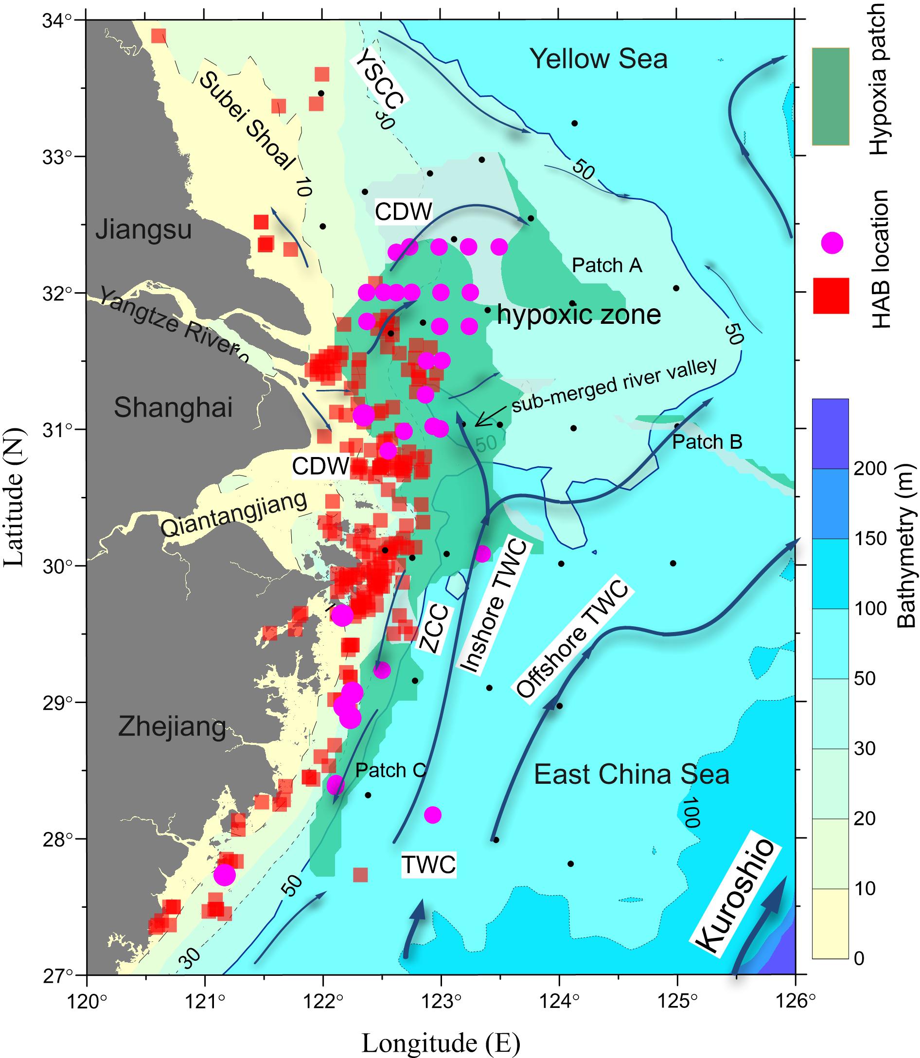
Figure 1. The circulation pattern (arrows) in the coastal and shelf waters adjacent to the Changjiang Estuary. The expansion of the Changjiang Diluted Water (CDW) off the estuary depends on interplays among the Yellow Sea Coastal Current (YSCC) from the north, the Zhejiang Coastal Current (ZCC) from the south, the inshore and offshore Taiwan Warm Current (TWC) originated from the strong upwelling north of Taiwan and other forcing. The distributions of harmful algal blooms (HABs) during 1979–2009 (Liu et al., 2013) are shown by red squares and those for 2010–2016 by pink circles (Bulletin of China Marine Environment; Supplementary Table S2). The composite distribution of the hypoxic zones in this region since the early 1990s is depicted with green shading (Supplementary Table S1). Black dots represent the station locations for the three repeated surveys referred to in this study.
Beyond leading to higher phytoplankton standing stock (Zhou et al., 2008), this coastal eutrophication has resulted in a shift in the phytoplankton community composition in the East China Sea (ECS) (Zhou et al., 2001, 2008; Wang et al., 2016; Yu and Liu, 2016). In particular, there has been an increase in harmful algal blooms (HABs), including the toxic Karenia mikimotoi and Alexandrium catenella as well as the ecosystem-disruptive species Prorocentrum donghaiense and Noctiluca scintillans (Figure 1; Liu et al., 2013; Dai et al., 2014; Lu et al., 2014; Yu and Liu, 2016). Along with changes in plankton assemblages has come the annual development of large-scale hypoxia in the region (Li et al., 2002; Chen et al., 2007; Wei et al., 2007; Wang, 2009; Zhou et al., 2010; Ning et al., 2011; Zhu et al., 2011, 2016; Liu et al., 2012; Wang et al., 2012, 2016, 2017; Zhu et al., 2017; Luo et al., 2018; Supplementary Figure S1 and Supplementary Table S1). However, the quantitative linkages among these large-scale changes in the frequency and species composition of phytoplankton blooms, dissolved oxygen depletion, and the distribution and expansion of hypoxic areas are poorly understood, mainly due to the limitations of ship-based, discrete, and intermittent sampling of this highly dynamic coastal environment (Figure 1).
Like other anthropogenically affected coastal regions (Silva et al., 2016), marine environmental issues off the CJE demand an enhanced mechanistic understanding of the physical–biogeochemical processes to enable better forecasting of hypoxic conditions (Zhang et al., 2018). In this work, we use a coupled physical–biogeochemical model to explore the relationship between the spatial–temporal variability of high-biomass phytoplankton production and offshore hypoxia and to reveal the causal linkages among physical processes, nutrient cycling, phytoplankton production, and hypoxia at both seasonal and single-event timescales in the ECS. Although our understanding of this complex system is not yet complete, the findings here help to validate this coupled model approach and its predictive capacity. We hope that this approach can be adopted to support the design of ecosystem restoration strategies to mitigate hypoxia off the CJE.
Materials and Methods
Field and Satellite Data
Three repeated multidisciplinary field surveys with coarsely spaced sampling stations were carried out off the CJE (122.0–125.0° E, 27.5–33.5° N) during June 2–11 (Jun cruise), August 19–30 (Aug cruise), and October 3–13 (Oct cruise) in 2006 (Figure 1, dots). Detailed information about these cruises are given in Zhou et al. (2010) and Zhu et al. (2011). A single intensive survey with high-resolution sampling stations into the Changjiang and in the adjacent coastal region was conducted during July 13–August 23, 2006 (Gao et al., 2011; Li et al., 2011). Additional cruise observational data were included from May (May 10–June 3) (Chen et al., 2008) and September (Zou et al., 2008; Wang et al., 2012) cruises in 2006 to facilitate our understanding of the seasonal development of hypoxia.
Vertical profiles of temperature and salinity were measured using a Sea-Bird conductivity, temperature, and depth (CTD). Discrete water samples were collected using a CTD rosette at near surface, 10 m, within the pycnocline, and near bottom. Chlorophyll a (Chl a) was measured by extraction into 90% acetone using the acidification method (Holm-Hansen et al., 1965). Remotely sensed Chl a data were used to resolve the high spatial–temporal variability of phytoplankton biomass. Daily level 3 surface Chl a data from the GlobColour1 (hereafter, SAT Chl a), i.e., SeaWiFS, MERIS, and MODIS, were extracted for the study region and showed good agreement with in situ observations (Supplementary Figure S2A). A composite of these SAT Chl a datasets using the weighted averaging algorithm among different satellite sensors was used from the GlobColour. Chl a was overestimated by the satellite where in situ Chl a was <10 μg/L, but was underestimated where in situ Chl a was >10 μg/L (Supplementary Figure S2A). In spite of that, SAT Chl a showed overall good agreement (r = 0.68) with in situ Chl a data and the root mean squared difference (RMSD) of 0.39 μg/L (Supplementary Figure S2A).
Vertical profiles of dissolved oxygen were measured with a high-accuracy dissolved oxygen sensor (Sea-Bird SBE43), mounted on the CTD rosette. Dissolved oxygen was also measured from the sampled water by the titration method (Bryan et al., 1976) at discrete depths (surface, two or three depths spanning the pycnocline to improve the sampling resolution according to the pycnocline thickness, and near the seabed) to verify sensor accuracy (Supplementary Figure S2B). The sensor-measured dissolved oxygen data were validated with the titrated dissolved oxygen data and showed a high correlation coefficient of 0.97 with a low RMSD of 0.53 mg/L. Then, the high-vertical-resolution sensor-measured dissolved oxygen data were calibrated based on a linear regression y = 0.9063x + 0.7265. Here, y represents the calibrated sensor-measured dissolved oxygen (hereafter, DO) and x represents the titrated dissolved oxygen (Supplementary Figure S2B).
Physical–Biogeochemical Model
The physical processes were simulated by a customized Regional Ocean Modeling Systems (ROMS) (Shchepetkin and McWilliams, 2005; Haidvogel et al., 2008). The model covers the domain of 117.5–132.0° E and 23.5–41.0° N, with a curvilinear grid and an approximately homogeneous 4-km horizontal resolution and 30 vertical levels. The model was spun up for 3 years starting from a climatological January mean that was derived from multiyear observations between 1958 and 1987 (Chen, 1992) and driven by Comprehensive Ocean–Atmosphere Data Set (COADS) climatological monthly forcing (Da Silva et al., 1994). The last-year model output was used as the initialization for the realistic run of 2006, for which the surface heat and freshwater fluxes were obtained from the 3-hourly European Centre for Medium-Range Weather Forecasts (ECMWF) ERA-Interim (Dee et al., 2011). The wind stress was calculated from wind vector data as described by Large and Pond (1981), and the wind vector data were from the Blended Sea Winds (Zhang et al., 2006; Peng et al., 2013), which provide daily 0.25° gridded ocean surface vector wind based on multiple satellite observations. The same wind stress was also used for analyzing the wind mixing. Boundary conditions such as temperature, salinity, velocity, and sea surface elevation were extracted from Global Hybrid Coordinate Ocean Model (HYCOM) climatology averaged from 1979 to 2003 and HYCOM realistic run for 2006 (Kelly et al., 2007), respectively. Both the climatological run and the realistic run include the Changjiang runoff (Table 1). See Zhou et al. (2015) for more details on the circulation model setup and validation. The realistic run of 2006 was driven by the realistic forcing repeatedly for two cycles, and the last cycle output was analyzed in this article.
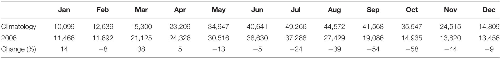
Table 1. Comparison of the monthly Changjiang runoff (unit: m3/s).
Observational evidence indicates that diatom blooms are the major source of organic matter export leading to hypoxia off the CJE (Wang et al., 2017). The 13-component carbon, silicate, and nitrogen ecosystem (CoSiNE) model was thus selected, which includes: silicate, nitrate, phosphate, ammonium, picophytoplankton, diatoms, microzooplankton, mesozooplankton, small/suspended particles, large/sinking particles, oxygen, total CO2, and total alkalinity. The detailed descriptions of the CoSiNE model are given in Chai et al. (2002) and Xiu and Chai (2014). For more details on the CoSiNE model setup and validation for the ECS and the CJE, see Zhou et al. (2017). All biological components were coupled online with physical processes, such as advection and diffusion. The simulated Chl a is referred to as modeled Chl a (MOD Chl a) to distinguish it from satellite-determined Chl a (SAT Chl a) and water column measurements (in situ Chl a).
Results
Modeled Chl a and Currents
The spatial patterns of the bimonthly MOD Chl a (Figures 2A–D) were in reasonable agreement with the composite bimonthly SAT Chl a over the May through October study period, as was the magnitude of production in July and August. Both MOD Chl a and SAT Chl a showed a strong concentration gradient between the nearshore and offshore regions. The MOD Chl a showed high production mostly occurring off the CJE and adjacent nearshore regions. The simulations showed that phytoplankton production in the area had significant seasonality and peaked in July–August, which was similar to those of SAT Chl a. There were some mismatches between MOD Chl a and SAT Chl a. The spring phytoplankton production off the Zhejiang coast occurred later in the simulations than that of the satellite data (Figure 2E). The high-concentration Chl a tongue extending from the river mouth to beyond the 20-m isoline was underestimated in the simulations (Figures 2F,G). Meanwhile, the modeled Chl a levels were overestimated compared to SAT Chl a values during May–October, particularly in the nearshore regions such as the Subei Shoal and the Qiantangjiang Estuary (Hangzhou Bay) (Figures 2F–H).
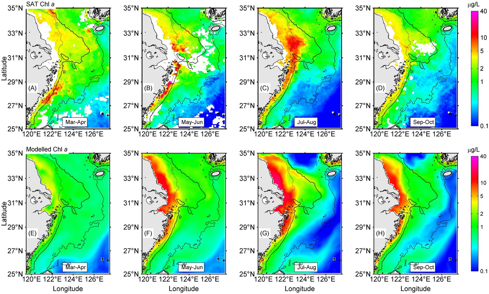
Figure 2. The spatial distributions of bimonthly mean satellite (SAT) Chl a and modeled Chl a in the study region from March through October. The contours are isobaths of 20 m (dotted), 50 m (solid), and 100 m (dashed). Satelllite measured Chl a averaged between March to April (A), May to June (B), July to August (C) and September to October (D). Modelled mean Chl a in March to April (E), May to June (F), July to August (G) and September to October (H).
The model-simulated current field suggested a prevailing monsoon-driven northeastward current at all layers from the surface to near bottom, namely, the TWC as suggested by Beardsley et al. (1985), Su and Pan (1987), and Su (1998), showing two branches in the southern ECS (Figure 3) similar to the current structure presented by Yuan et al. (1987), Ichikawa and Beardsley (2002), and Xuan et al. (2017). The nearshore branch was along the Zhejiang coast and separated from the offshore branch south of 28° N. The nearshore branch again bifurcated into two parts south of 30.5° N, with one part moving northward and pushing the Changjiang Diluted Water (CDW) to north of the river mouth until 33.5° N, and there the two parts turned together eastward and southeastward. The offshore part turned eastward at 30.5° N and finally joined the Cheju Warm Current, as suggested by Lie et al. (2000). The northeastward and later southeastward of the CDW tongue north of the river mouth was a well-recognized feature in previous in situ observations (Mao et al., 1963; Beardsley et al., 1985). The simulated current fields at different depths showed some similar patterns, but also significant differences off the CJE. For instance, the bottom layer suggested a notable northwestward onshore flow right outside of the river mouth, while the surface layer showed a bifurcation that extended northeastward and southeastward, respectively. The bottom layer also produced a band of convergence close to the 50-m isobath northeast of the river mouth, and at the convergent band place the CDW at the surface turned eastward and then southeastward. In addition, the 30-m and bottom layers seemed to have more trend of eastward movement in the offshore of the CJE.
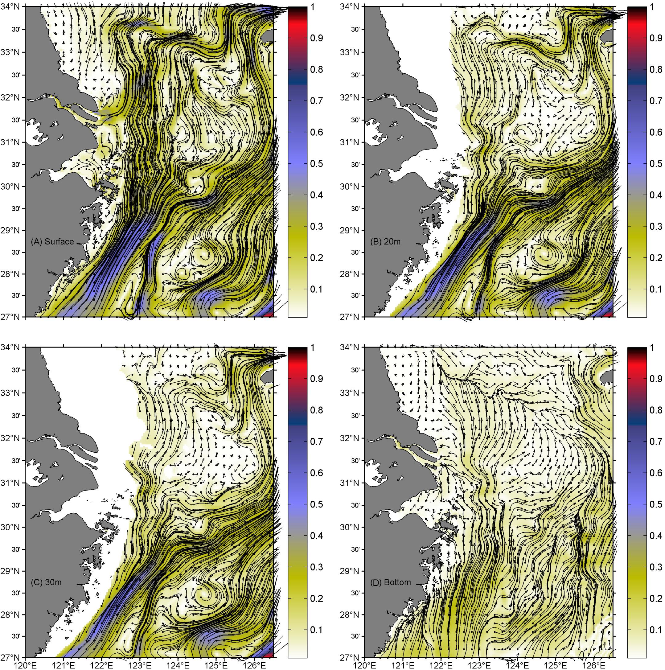
Figure 3. Simulated current fields at different depths off Changjiang Estuary (CJE) in July 2006. Surface (A), 20 m (B), 30 m (C), and near-bottom (D) layers. The current vectors drawn in this figure were selected in a search radius of ∼20 km. Shading represents the current magnitude (in meters per second).
Observed High Chl a Patch at the Surface and Hypoxia at the Seabed
Spatial distributions of the monthly mean SAT Chl a and DO in bottom waters are shown in Figure 4. SAT Chl a was elevated at the surface during May in a narrow band-like region along the coast from Zhejiang (34 μg/L) to the river mouth of the Changjiang (36 μg/L), centered long the 50-m isobath in the submerged ancient river valley (Figure 4A). The DO in the bottom water likely had not yet reached hypoxia (Figure 4A) based on a limited dataset showing the lowest DO concentration to be 4.96 mg/L (Chen et al., 2008).
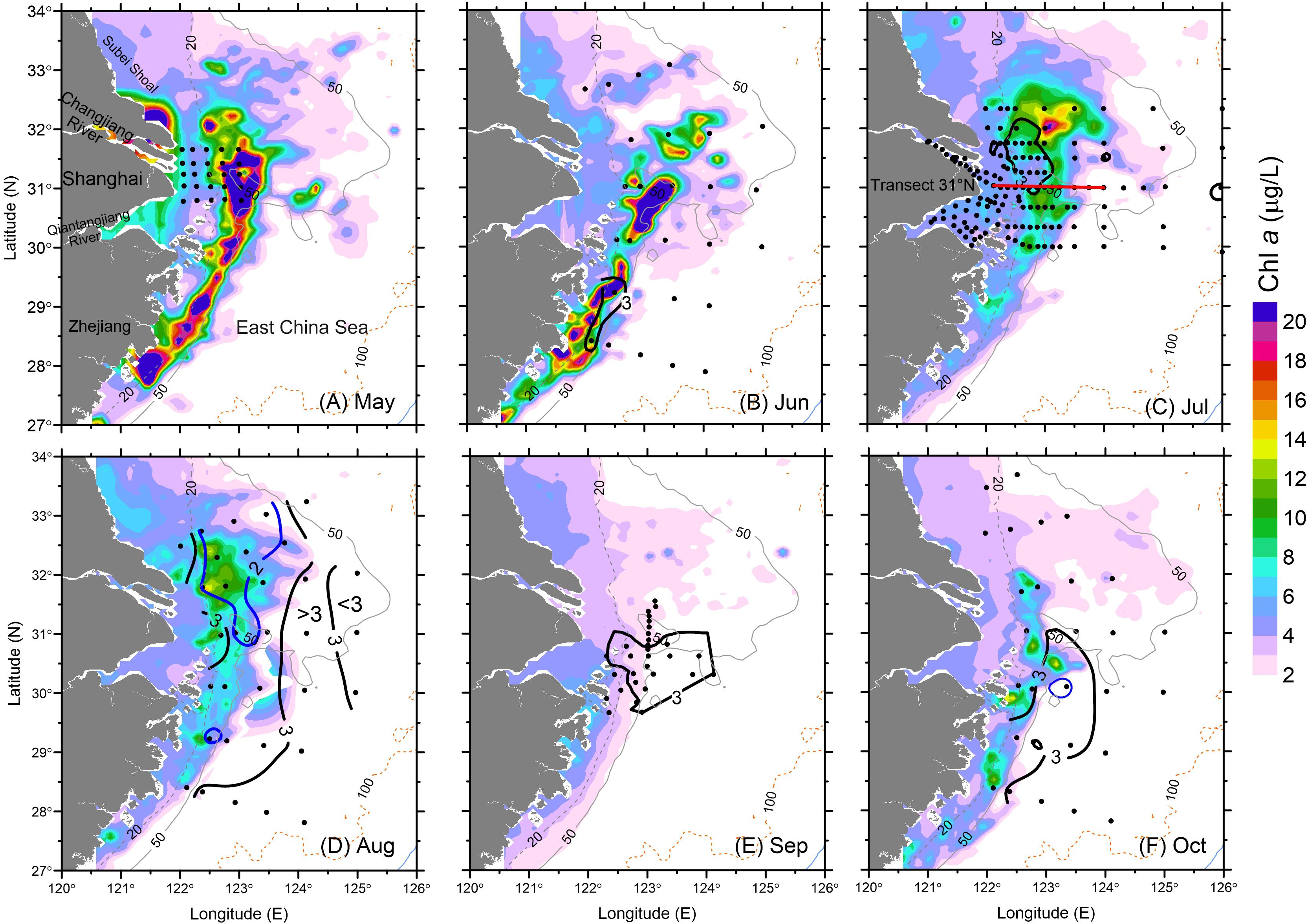
Figure 4. Surface (SAT) Chl a and bottom water DO (thick contour) during May–October 2006: (A) May, (B) June, (C) July, (D) August, (E) September and (F) October. The hypoxic zone during September was digitized based on Wang et al. (2012). Black contours represent DO of 3 mg/L and blue contours are for DO of 2 mg/L. Dots represent sampling stations during the corresponding cruise.
A high concentration of SAT Chl a continued to occur in June at the surface over an in situ observed hypoxic patch of bottom waters along the Zhejiang coast south of the CJE. The SAT Chl a concentration along the Zhejiang coast (32 μg/L) was similar to that in May, as were the high in situ Chl a levels over the submerged river valley (see Figure 1) off the CJE (40 μg/L) (Figure 4B). The peak in situ Chl a measured during the cruise (10.5 μg/L) occurred on June 10, which was approximately 25% of the peak value estimated by the satellite on June 21. Episodic high Chl a levels were observed both in situ and from satellite primarily off the Zhejiang coast during both May and June with less variation than in the other regions, consistent with previous observations (Zhou et al., 2003; Zhao et al., 2004; Liu et al., 2013).
In contrast to June, high SAT Chl a (i.e., surface waters) during July coincided with low DO concentrations in bottom waters very close to the river mouth (Figure 4C). The high in situ Chl a was also observed by the cruise in July (not shown). These cruise data, benefitting from the greater sample station density in the CJE, clearly show the co-occurrence of high phytoplankton biomass and low DO, mainly between the 20- and 50-m depth east of the river mouth. Smaller patches of hypoxia were measured not only in this region but also to the east (126° E, 31° N and 124° E, 31.5° N) in late July and early August. The highest in situ Chl a concentration measured in July was 21.3 μg/L, in close agreement with the SAT Chl a values (20 μg/L). The Changjiang and Qiantangjiang River estuaries had relatively low in situ Chl a near the river mouth in July (5 μg/L) compared to that occurring in May.
The high SAT Chl a concentration pattern (peak at 15 μg/L) in August was similar to that observed in July; in contrast, the low DO zone expanded significantly in both meridional and zonal directions (Figure 4D). DO concentrations were <3 mg/L across a spatial zone of 77,100 km2, or about 10 times of the hypoxic area observed in July, and hypoxia was also more intense, with the minimum DO deceasing from 2.0 mg/L in July to 1.0 mg/L in August. Although the hypoxic region expanded and covered most of the study area, except close to the 100-m isobath, peak in situ Chl a concentrations decreased to 16.1 μg/L and were slightly lower than those in July. SAT Chl a showed a similar decreasing trend during August.
September brought a drastic decrease in SAT Chl a concentrations, and presumed ventilation of subsurface waters led to some relaxation in hypoxic intensity and contraction of the hypoxic zone. The minimum DO increased to 2.0 mg/L (Zou et al., 2008), and hypoxia north of the river mouth disappeared (Wang et al., 2012; Figure 4E). SAT Chl a in the study region showed a reduction by ∼30% relative to August, and the spatial extent of high biomass (Chl a > 10 μg/L) was less than 5% of that measured in August.
Moderately high SAT Chl a remained at the surface in the area north of the CJE during October, slightly lower than that in August but much higher than that in September (Figure 4F). The high Chl a patch along the Zhejiang coast that disappeared in September appeared again in October at more moderate levels. The peak in situ Chl a during the cruise (27.7 μg/L) was twice that of the SAT Chl a (14.0 μg/L) averaged over the larger area. The spatial extent of the hypoxic zone increased substantially, from 16,400 km2 in September to 26,500 km2 in October, and extended from the Zhejiang coast to the northern tip of the submerged river valley (Figure 4F).
As noted, the spatial distribution of high Chl a biomass did not match that of hypoxia during the summer–fall stratified period, illustrating a complex interaction between biological and physical processes. This variation is illustrated by the presence of minor hypoxic patches in regions with low Chl a (Figures 4C,D). In addition, the highest Chl a at the surface on the 31° N transect occurred along the outer edge of the upper front immediately outside of the river mouth, while the minimum DO occurred in the shore side of the front (Figure 5). Indeed, hypoxic bottom waters were overlain by low levels of Chl a biomass more often than that of high-biomass waters, according to the comparison of both SAT Chl a and in situ Chl a at the surface with DO measurements at the bottom layer (Figure 6). Given that advection would have contributed to the variable distribution of the high-biomass phytoplankton patches, the annual spatial dynamics of surface phytoplankton biomass was compared to the ROMS-determined spatial dynamics of bottom hypoxic waters in the study region.
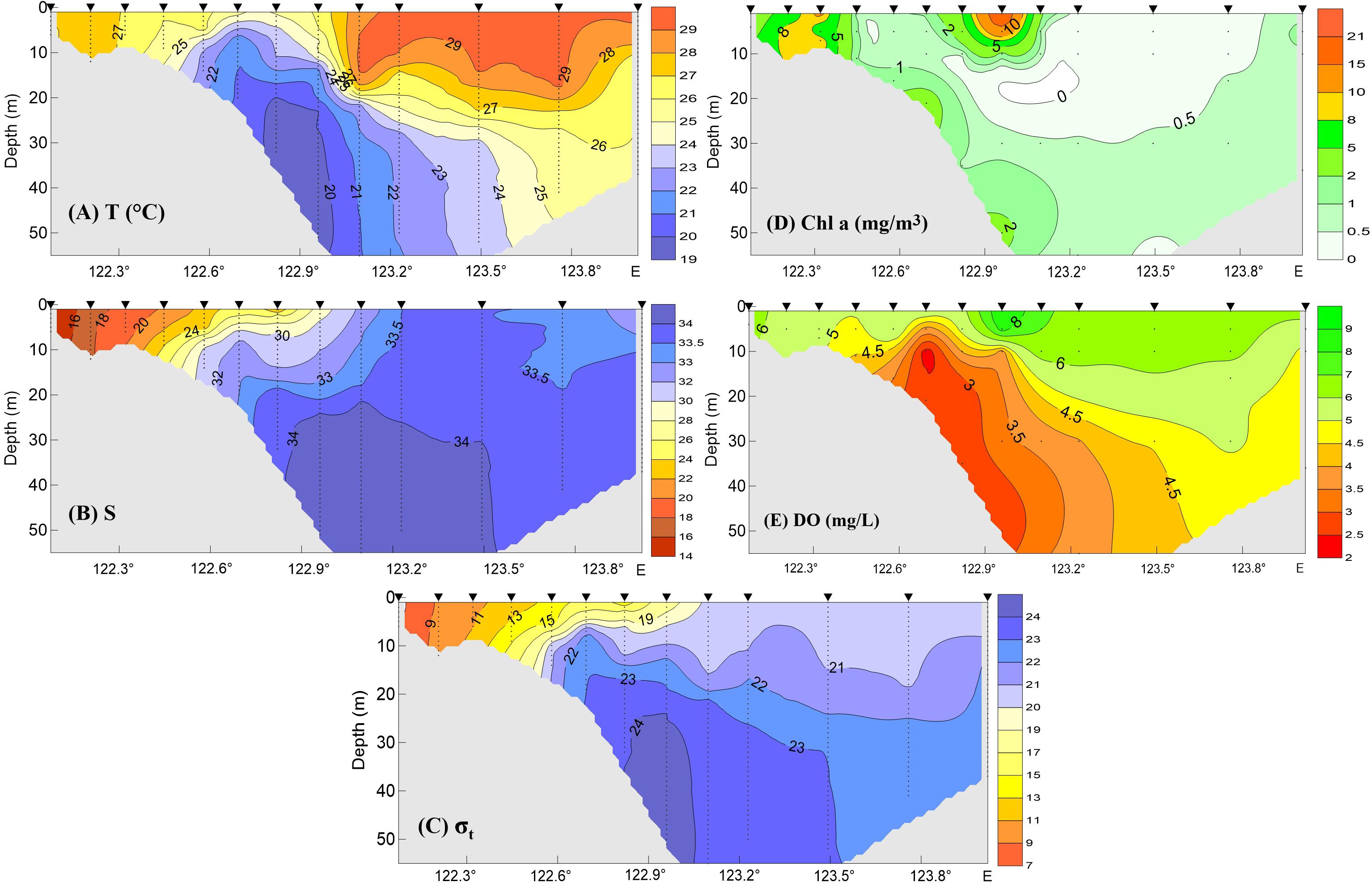
Figure 5. Temperature (A), salinity (B), density anomaly by minusing 1000 kg/m3 (C), Chl a (D), and DO (E) observations along the 31° N transect shown in Figure 4C during the intensive survey on August 12–15, 2006. Triangles on the top marked the sample stations.
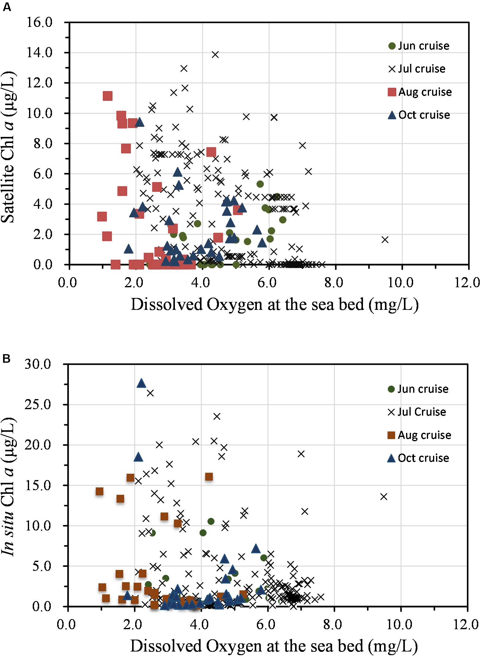
Figure 6. Relationship between phytoplankton production (Chl a) at the surface and dissolved oxygen at the bottom layer based on field measurements in 2006. (A) Satellite Chl a and (B) in situ Chl a.
Modeled Hypoxic Zone
As a first step, the low-level DO distribution during the year was extracted from the model to identify the most probable regions of oxygen depletion (Figure 7A). The modeled low DO concentration generally occurred below 20-m depth. To the north of the CJE, the model results suggested that oxygen depletion was distributed on both the western and eastern sides of the 30-m isobath, with the exception of an isolated low-DO patch further offshore at the 50-m isobath. To the south of the river mouth, the simulated oxygen depletion occurred along the coast between the 20- and 50-m isobaths and at the submerged river valley deeper than 50 m (Figure 7A).
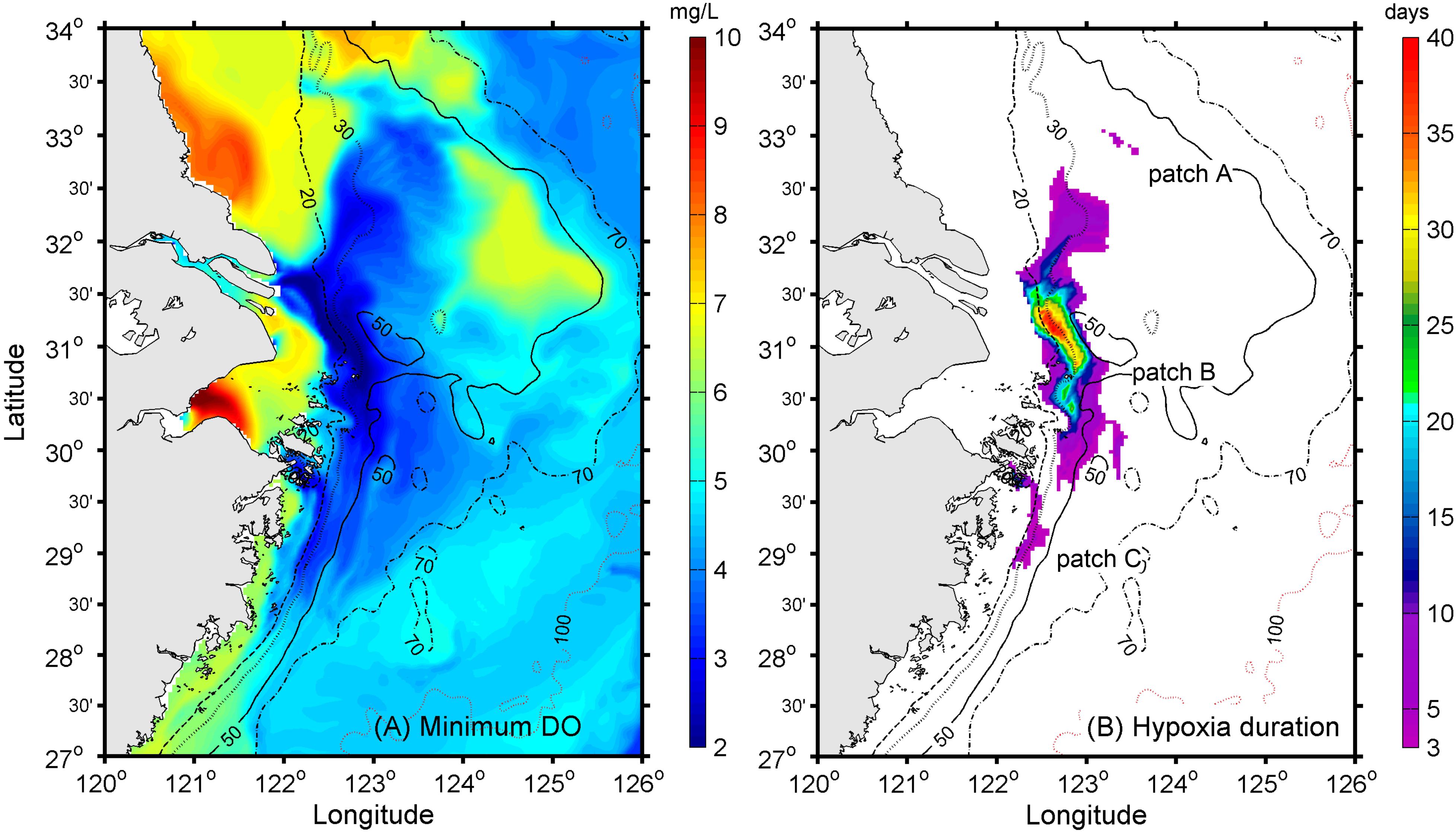
Figure 7. (A) Simulated minimum DO concentrations during the hypoxic period and (B) simulated hypoxia duration in days, with the colored regions representing the maximum hypoxic zone (MHZ) with three spatially distinct patches.
The maximum hypoxic zone (modeled MHZ) during the year, defined as the assemblage of all grid points where hypoxia was detected in the model—see Zhou et al. (2017) for a detailed discussion—was extracted to show the largest extent of hypoxic zone. The modeled MHZ existed as a narrow elongated band from the southern Jiangsu coast to the northern Zhejiang coast (Figure 7B). Three separate patches could be identified from the modeled MHZ, likely associated with the diversion of the CDW. Running north to south, the first hypoxic water patch, Patch A, lay approximately 300 km northeast of the river mouth near the 50-m isobath (Figure 7B). It had a long-duration core, reflecting the fact that the CDW passed through this region over most of the season. The second most intense patch, Patch B, lay meridionally distributed in the offshore vicinity of the CJE, while the third hypoxic patch, Patch C, occurred to the south along the Zhejiang coast (Figure 7B).
To better understand how organic matter production in the upper layers is linked to hypoxia, the modeled oxygen depletion under the pycnocline was compared with the time series of SAT Chl a inside and outside the modeled MHZ within the rectangular zone (120.5–128.5° E, 25.5–34.5° N) (Supplementary Figure S3A). The annual mean SAT Chl a within this MHZ was almost three times larger than that outside the region, consistent with hypoxia being attributable to the decay of nutrient-driven phytoplankton production in the overlying waters. There was a positive correlation (r = 0.52) between the fluctuations of the modeled Chl a and SAT Chl a within the MHZ. These SAT Chl a data show that phytoplankton biomass increased slowly from January through April and peaked with a bloom during May–June, followed by lower but still substantial chlorophyll levels in July–August. The modeled Chl a concentrations followed the measured SAT Chl a from January through April, did not capture the bloom in May–June, but reached maximum levels in late July that matched the SAT Chl a concentrations (Supplementary Figure S3A). Thereafter, there was generally good quantitative agreement between the SAT Chl a and modeled Chl a, with diminishing concentrations from August to mid-September, followed by a smaller phytoplankton bloom during October, and then decreasing to low winter values by December. Discrete measurements of the in situ Chl a >10 μg/L during the four cruises of this study (June through October) showed the same general pattern (Supplementary Figure S3B). Augmenting these data with the most current findings of the Bulletin of China Marine Environment (for 2006) also shows a vast bloom extent in May–June.
Modeled Physical–Biogeochemical Processes During Phytoplankton Blooms and Hypoxia
The time series of wind-induced mixing, stratification, nutrients, and phytoplankton succession were investigated in the model domain, using averaged values over the entire modeled MHZ, to investigate the linkages of physical processes, nutrient cycling, phytoplankton blooms, and high Chl a with hypoxia (Figure 8).
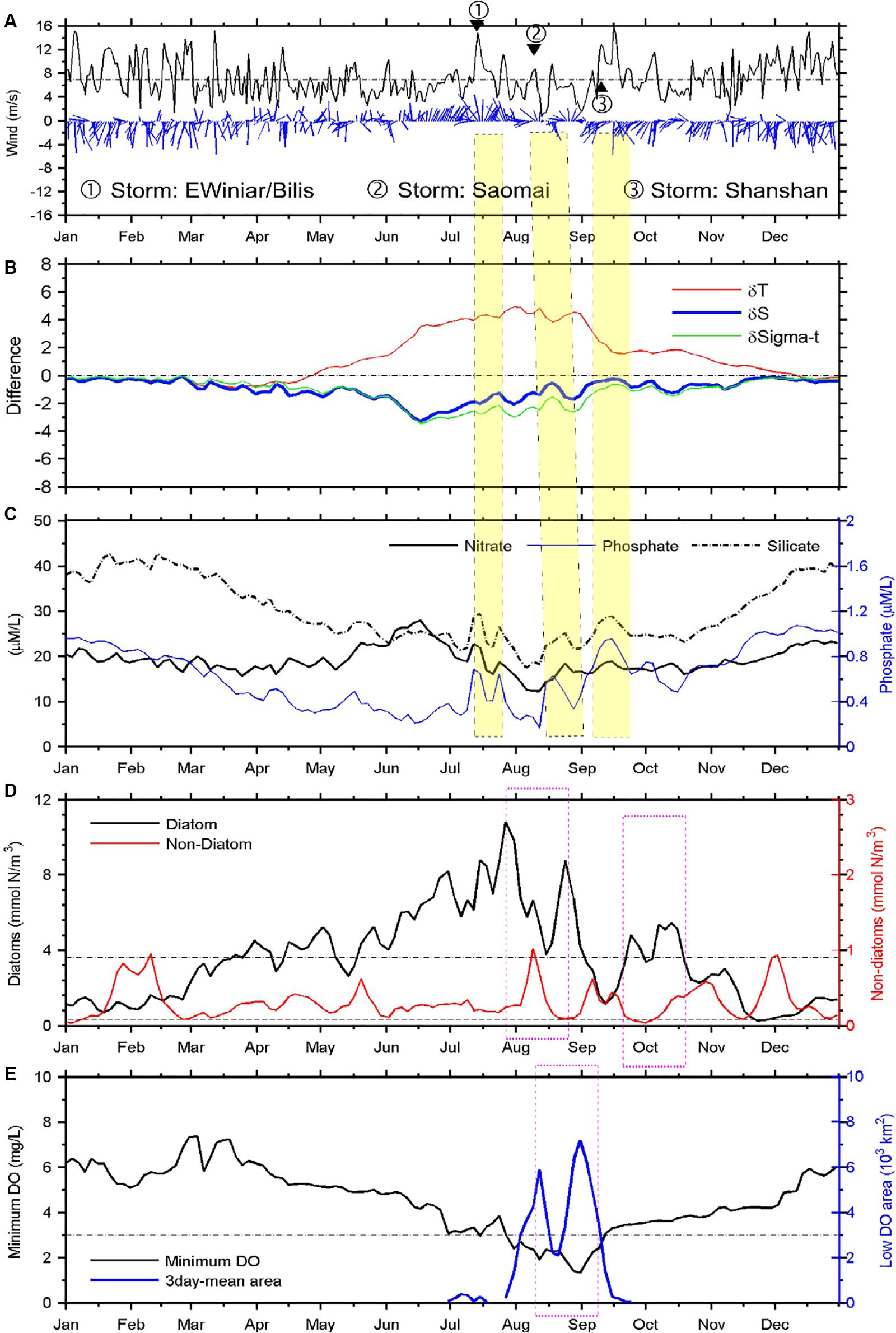
Figure 8. Time series of satellite-observed wind and modeled variables. Wind vectors and speed (A), stratification (B), nutrients at the surface (C), phytoplankton at the surface (D), and hypoxia at the bottom (E). Stratification, nutrients, phytoplankton concentrations, and minimum DO concentration represent the simulated averages within the study area. The simulated phytoplankton biomass concentrations of diatoms and non-diatoms are in nitrogen units (Chai et al., 2002).
The study area is dominated mostly by the monsoon wind patterns, with strong northerly wind occurring during the fall and winter, substantially weaker southerly winds during the summer, and more variable wind directions during the late spring and September–October transitional period (Figure 8A). The averaged wind speed usually was less than 7 m/s from late spring to summer, with the exception of sporadic tropical storm or typhoon events (depicted by the numbered circles in Figure 8), where wind speeds averaged up to ∼14 m/s within the study area.
The stratification intensity was approximately represented by the surface to bottom difference of density, temperature, and salinity. The weaker winds during the summer generally were not able to disrupt the density stratification of the water column, with only some slight reduction, e.g., in mid-August. The significant and rapid loss of stratification occurred only in early September, associated with the strong Tropical Storm Shanshan and subsequent strong northerly wind (Figures 8A,B). Both temperature and salinity difference contributed significantly to the stratification; however, their temporal patterns varied in complex ways, with salinity difference decreasing when the temperature difference increased during mid-June to early August (Figure 8B). The reduced contribution of salinity to stratification after mid-June was related to the reduction in riverine input (Table 1). The salinity difference above and below the pycnocline peaked in mid-June instead of August, in associated with the maximum Changjiang runoff in 2006 (Table 1), which was unusual compared to the climatological mean discharge. The increased runoff during late May to June coincided with an increase in the mean nitrate concentrations in surface waters (Figure 8C), but not in phosphate or silicate due to the phytoplankton uptake of these nutrients during the spring blooms. That is, a greater replenishment of N than P or Si in runoff waters led to more rapid depletion of the latter two as a consequence of phytoplankton growth.
The enhanced vertical mixing that accompanied the strong wind events in July, August, and September increased the modeled nutrient flux into surface waters (Figures 8C,D). The simulated diatom growth increased sharply immediately following these wind-induced mixing events, but reached maximum biomass ∼1–2 weeks after the wind events Figure 8D). These two largest diatom bloom events were followed by two large hypoxia events ∼2 weeks later, consistent with the model findings (Figure 8E).
The model also shows the succession of diatoms and non-diatoms, where increases in non-diatom biomass followed decreases in diatom biomass (Figure 8D). The onset of non-diatom blooms occurred rapidly on termination of the diatom blooms during mid-April and mid-May, mid-August, mid-September, late October, and in December. The model-derived time lag between the diatom and non-diatom blooms is within a reasonable range of the field observations (data not shown). Diatom concentrations decreased to a very low level after October, and no blooms occurred during mid-November to late January.
A Hovmöller diagram (which displays time on one axis and distance on the other) along a more or less meridional transect was extracted from the simulation to examine the relationship between high-biomass phytoplankton production and oxygen depletion below the pycnocline (Figure 9). The transect cut through the middle of the long side of the modeled MHZ, with its origin set at the southern end. For simplicity, the vertically integrated diatom concentrations are shown, which illustrate a series of diatom blooms between March and November. Intensive blooms occurred on the along-shore transect at the end of June (Figure 9A). By mid-July, the vertically integrated phytoplankton production reached 2 mol C/m2, assuming a C:N ratio of 9.88 (Harrison et al., 1977), and while oxygen began to be depleted in bottom waters at this time, the area and intensity of oxygen depletion did not enlarge substantially until the end of August/early September. The expansion of hypoxia was enhanced by the second and third high diatom biomass events in late August. The time lag was 1–18 days, but varied at different distances along the transect (Figure 9). The lag phase generally decreased south of the river mouth and increased north of the river mouth, except for the region where no significant diatom blooms occurred.
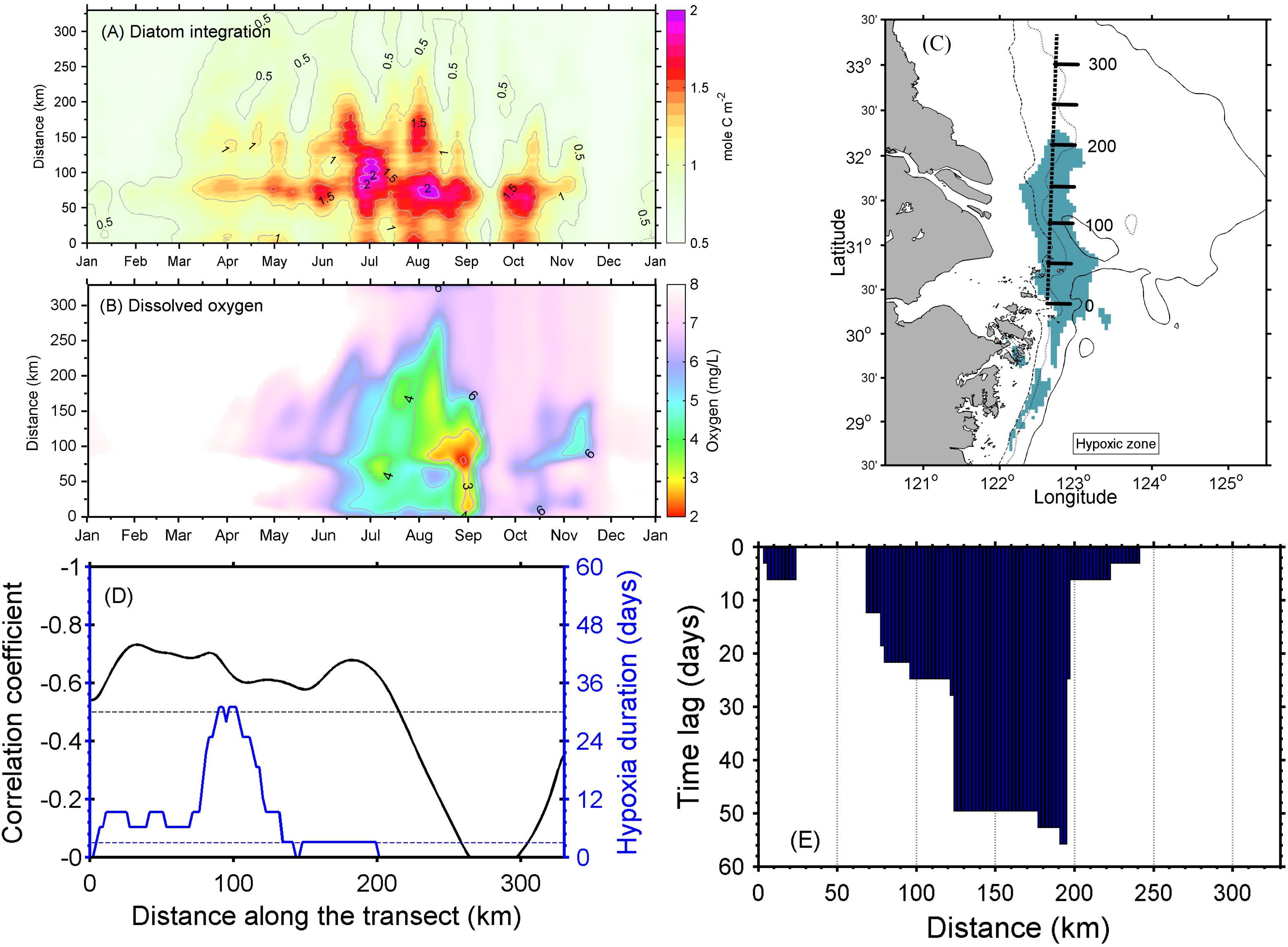
Figure 9. (A) Hovmöller diagram of the vertically integrated diatom concentration and (B) dissolved oxygen at the seabed along the transect. (C) The transect location with its origin set at the southern end and distance labeled in kilometers. (D) Correlation coefficient between the vertically integrated diatom concentration and dissolved oxygen (DO) at the seabed (black curve), with hypoxia duration days (blue curve). (E) Lagged correlation analysis shows the days lagged between the vertically integrated diatom concentration and DO at the seabed.
Further correlation analysis showed that there was reasonable spatial agreement between diatom abundances and DO at the bottom layer in the model. The inverse correlation between vertically integrated diatom abundance and DO in bottom water is −0.60 for the whole transect (Figure 9D), while the coefficient is −0.58 between diatoms at the surface layer and DO at the near-bottom layer (Supplementary Figure S4). This inverse correlation was always greater than −0.5 along the transect where both hypoxia and diatoms showed significant concentrations, i.e., the distance from 50 to 150 km, and the strongest correlation was −0.73 at 15 km from the southern end of the transect (Figure 9D). The phase lag analysis showed that the oxygen depletion mostly occurred a week to 2 months later after the diatom blooms in this transect, where the correlation is >0.5 (Figure 9E). However, this was not always the case. The relationship between oxygen depletion and diatom abundance was significantly correlated at the distance around 50 km along the meridional transect shown in Figure 9C, but showed no remarkable time lag.
The model also shows the succession of diatoms and non-diatoms, where increases in non-diatom biomass followed decreases in diatom biomass (Figure 8D). The onset of non-diatom blooms occurred rapidly during mid-April and mid-May, respectively, at the termination of the diatom blooms. The non-diatom blooms occurred throughout most of the record, e.g., February, in mid-May, early August, and in late October. Decreases in the integrated concentrations of both diatoms and non-diatoms over the stratified period occurred after the strong northerly wind event, e.g., from August to October. Diatom blooms peaked approximately 1–2 weeks after the wind-mixing events, while non-diatom blooms generally appeared 1–2 weeks after the diatom blooms. The phase lag between these two blooms is within the reasonable range of field observations (Lu et al., 2000). A similar succession of microalgae blooms was also revealed in other modeling studies of this region (Zhou Z et al., 2017). The simulated diatom concentrations decreased to very low levels after October, and no blooms occurred during mid-November to late January. Note that the two phytoplankton functional groups differed in their sinking rates, with the diatom detritus sinking velocity being ∼25 m each day (i.e., reaching the seabed within ∼1 day compared to the lower rate of 15 m each day for the non-diatoms).
Discussion
Coupling and Decoupling Between Surface High-Biomass Diatom Blooms and Bottom Hypoxia
Forecasting the timing, position, spatial extent, and duration of hypoxic zones in the coastal and shelf regions surrounding the CJE is compounded by the dynamic linkages among the physical, chemical, and biological processes. The model results suggest that high-biomass phytoplankton production in this region is regulated by seasonal and intra-seasonal fluctuations in both the anthropogenic nutrient-rich Changjiang (Yangtze River) diluted water and the natural nutrient influx carried by several shelf currents. The model results also revealed that the event-scale variability in the resulting subsurface hypoxia is characterized by episodic disruption of the pycnocline associated with weather events, which enhances nutrient flux to surface waters and can trigger more severe hypoxia in the region. There exists a straightforward coupling between high-biomass diatom blooms and low DO in underlying waters near the core hypoxic region immediately adjacent to the mouth of the estuary; on average, the modeled phytoplankton Chl a biomass was approximately three times higher over the core hypoxic zone than in the surrounding regions (Supplementary Figure S3). However, there was also significant decoupling of production at the surface (or in the water column) and hypoxic zones during 2006, as seen from in situ observations (Figures 5, 6) and simulations (Figures 9A, 10). In general, subsurface hypoxia was not always correlated with Chl a biomass in the overlying waters across the broader region in the shelf sea outside of the CJE. Portions of the high-biomass blooms, or their underlying waters, often became detached from CJE and were advected along the coast and to the outer shelf (Figures 3, 10). Such episodes were poorly captured by ship monitoring surveys, resulting in an underestimation of the spatial extent of hypoxia (Supplementary Figure S3B). Adequate mechanistic-based forecast of the development of these hypoxic events requires quantitative integration of the physical and biogeochemical processes.
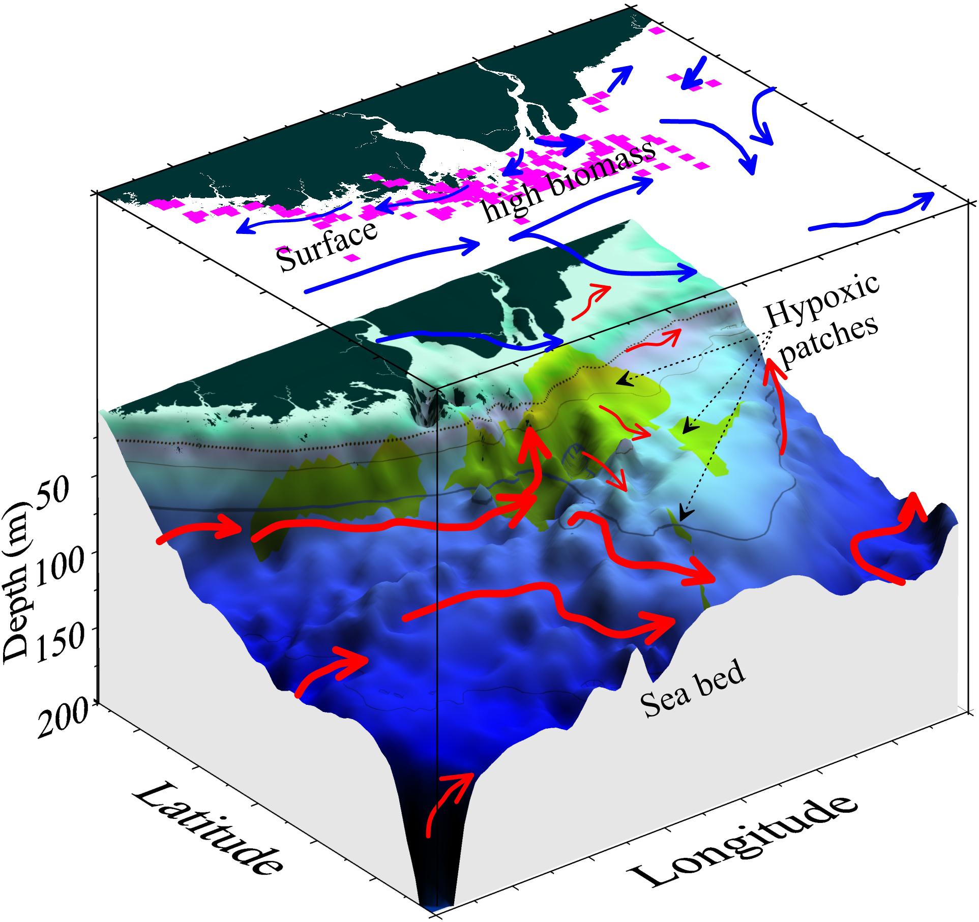
Figure 10. Schematic diagram of the coupling and decoupling between high-biomass phytoplankton production (pink squares) and subsurface hypoxic patches (green shading). The decoupling is mostly associated with different current structures at the surface (blue arrows) and subsurface off the estuary (red arrows). Note that the current magnitude might not be represented proportionally by the thickness of the arrow.
Our model findings showed that diatoms accounted for a large portion of the high Chl a biomass, consistent with in situ observations (Wang et al., 2017), and were the major organic matter export that led to DO consumption below the pycnocline. Based on our simulations, the hypoxia tends to occur 1–8 weeks later than the diatom blooms. The findings here demonstrate how combining remote sensing, numerical simulations, and ship survey data can provide a more comprehensive assessment of the development and evolution of high diatom biomass and hypoxic conditions in this region.
Management Implications
Traditionally, the monitoring and research of “red tides” in Chinese coastal waters has been administratively restricted to toxic algae blooms. However, high-biomass productions that lead to hypoxia also are recognized as an important aspect of HABs having substantial ecological impacts to pelagic and benthic systems. Hypoxia off the CJE has become a seasonal phenomenon, and one where the intensity and spatial scale of hypoxia have been expanding. The definition of HABs in Chinese coastal waters should be broadened beyond only toxin-producing organisms to take into account the hypoxia generated by these massive algal blooms in the CJE and other coastal regions. This change would require expansion of the traditional HAB monitoring from not only nearshore regions but also further offshore where hypoxic events also develop.
Conclusion
Abundant supplies of nutrients facilitate a continued presence of high-biomass phytoplankton production and their eventual settling in the region and finally lead to multiple patches of hypoxia. Model results support that there is a time lag of a few weeks between bottom hypoxia and surface diatom blooms. Our findings show that, in most cases, hypoxia was spatially linked to primary production in the overlying waters; however, organic detritus in subsurface waters also were transported offshore with different rates and directions compared to the surface waters in this physically dynamic region, producing offshore patches of hypoxic waters. Advection significantly expands the hypoxic zone relative to the high-biomass phytoplankton zone, generating spatially decoupled relationships between bottom hypoxia and phytoplankton production in surface waters.
Data Availability Statement
The datasets generated for this study are available on request to the corresponding author.
Author Contributions
FZ, FC, and MW designed the original ideas presented in this manuscript and coordinated integration of the modeling results and observational data. DH conceived the hypoxia projects and the intensive cruise. FZ, JX, XN, CL, and HL collected the field measurements. FZ, XM, CL, and PW analyzed the field data. FZ, MW, HX, and JS wrote the original manuscript draft. FZ, FC, and HX prepared the physical–biological coupled modeling. FZ, QM, and QZ analyzed the results. All authors contributed to refining this manuscript.
Funding
This study was supported by the National Key Research & Development Program of China (grant 2016YFC1401603), NSFC-Zhejiang Joint Fund for the Integration of Industrialization and Informatization (grant U1609201), Scientific Research Fund of the Second Institute of Oceanography, MNR (grants JT1704 and 14283), the Zhejiang Provincial Natural Science Foundation (grant LR16D060001), and the National Natural Science Foundation of China (grants 41876026, 41576007, and NORC2013-03).
Conflict of Interest
The authors declare that the research was conducted in the absence of any commercial or financial relationships that could be construed as a potential conflict of interest.
Acknowledgments
Field data and model outputs used for the figures and tables are available via contacting the first author. We thank Dr. Zuoyi Zhu for providing DO titration data for calibrating sensors used in the three regular surveys and thank Dr. Jianfang Chen and his team for calibrating DO sensors in the intensive surveys. We also thank NOAA for providing gridded wind vector product via ftp://eclipse.ncdc.noaa.gov/pub/seawinds/.
Supplementary Material
The Supplementary Material for this article can be found online at: https://www.frontiersin.org/articles/10.3389/fmars.2020.00259/full#supplementary-material
Footnotes
References
Anderson, D., Glibert, P., and Burkholder, J. (2002). Harmful algal blooms and eutrophication: nutrient sources, composition, and consequences. Estuaries 25, 704–726. doi: 10.1007/BF02804901
Anderson, D. M., Burkholder, J. M., Cochlan, W. P., Glibert, P. M., Gobler, C. J., Heil, C. A., et al. (2008). Harmful algal blooms and eutrophication: examining linkages from selected coastal regions of the United States. Harmful Algae 8, 39–53. doi: 10.1016/j.hal.2008.08.017
Beardsley, R. C., Limburner, R., Yu, H. S., and Cannon, G. A. (1985). Discharge of the Changjiang (Yangtze River) into the East China Sea. Cont. Shelf Res. 4, 57–76. doi: 10.1016/0278-4343(85)90022-6
Bryan, J. R., Rlley, J. P., and Williams, P. J. L. (1976). A winkler procedure for making precise measurements of oxygen concentration for productivity and related studies. J. Exp. Mar. Biol. Ecol. 21, 191–197. doi: 10.1016/0022-0981(76)90114-3
Carrick, H. J., Moon, J. B., and Gaylord, B. F. (2005). Phytoplankton dynamics and hypoxia in Lake Erie: a hypothesis concerning benthic-pelagic coupling in the central basin. J. Great Lakes Res. 31, 111–124. doi: 10.1016/s0380-1330(05)70308-7
Carstensen, J., Andersen, J. H., Gustafsson, B. G., and Conley, D. J. (2014). Deoxygenation of the Baltic Sea during the last century. Proc. Natl. Acad. Sci. U.S.A. 111, 5628–5633. doi: 10.1073/pnas.1323156111
Chai, F., Dugdale, R. C., Peng, T., Wilkerson, F. P., and Barber, R. T. (2002). One-dimensional ecosystem model of the equatorial Pacific upwelling system. Part I: model development and silicon and nitrogen cycle. Deep Sea Res. Part II Top. Stud. Oceanogr. 49, 2713–2745. doi: 10.1016/s0967-0645(02)00055-3
Chan, F., Barth, J. A., Lubchenco, J., Kirincich, A., Weeks, H., Peterson, W. T., et al. (2008). Emergence of anoxia in the California current large marine ecosystem. Science 319:920. doi: 10.1126/science.1149016
Chen, C. A. (1996). The Kuroshio intermediate water is the major source of nutrients on the East China Sea continental shelf. Oceanol. Acta 19, 523–527.
Chen, C. C., Gong, G. C., and Shiah, F. K. (2007). Hypoxia in the East China Sea: one of the largest coastal low-oxygen areas in the world. Mar. Environ. Res. 64, 399–408. doi: 10.1016/j.marenvres.2007.01.007
Chen, D., Zhang, L. X., Liu, H. Q., and Li, Z. E. (2008). Distribution characteristics and correlating factors analysis of dissolved oxygen in spring and summer in the Yangtze Estuary. Mar. Environ. Sci. 27(Suppl. 1), 49–53.
Chen, D. X. (ed.) (1992). Marine Atlas of Bohai Sea, Yellow Sea and East China Sea, Hydrology. Beijing: China Ocean Press, 13–96.
Cloern, J. E. (2001). Our evolving conceptual model of the coastal eutrophication problem. Mar. Ecol. Prog. Ser. 210, 223–253. doi: 10.3354/meps210223
Conley, D. J., Carstensen, J., Rtebjerg, G., Christensen, P. B., Dalsgaard, T., Hansen, J. L. S., et al. (2007). Long-term changes and impacts of hypoxia in Danish coastal waters. Ecol. Appl. 17, 165–184. doi: 10.1890/05-0766.1
Conley, D. J., Humborg, C., Rahm, L., Savchuk, O. P., and Wulff, F. (2002). Hypoxia in the Baltic Sea and basin-scale changes in phosphorus biogeochemistry. Environ. Sci. Technol. 36, 5315–5320. doi: 10.1021/es025763w
Conley, D. J., Paerl, H. W., Howarth, R. W., Boesch, D. F., Seitzinger, S. P., Havens, K. E., et al. (2009). Controlling eutrophication: nitrogen and phosphorus. Science 323, 1014–1015. doi: 10.1126/science.1167755
Da Silva, A., Young, A. C., and Levitus, S. (1994). Atlas of Surface Marine Data 1994, volume 1: Algorithms and Procedures, NOAA Atlas NESDIS 6. Washington, DC: U.S. Department of Commerce.
Dai, M., Guo, X., Zhai, W., Yuan, L., Wang, B., Wang, L., et al. (2006). Oxygen depletion in the upper reach of the Pearl River estuary during a winter drought. Mar. Chem. 102, 159–169. doi: 10.1016/j.marchem.2005.09.020
Dai, X., Lu, D., Guan, W., Wang, H., He, P., Xia, P., et al. (2014). Newly recorded Karlodinium veneficum dinoflagellate blooms in stratified water of the East China Sea. Deep Sea Res. Part II Top. Stud. Oceanogr. 101, 237–243. doi: 10.1016/j.dsr2.2013.01.015
Dai, X., Lu, D., Guan, W., Xia, P., Wang, H., He, P., et al. (2013). The Correlation between Prorocentrum donghaiense Blooms and the Taiwan Warm Current in the East China Sea-Evidence for the “Pelagic Seed Bank”, Hypothesis. PLoS One 8:e64188. doi: 10.1371/journal.pone.0064188
Dai, Z., Du, J., Zhang, X., Su, N., and Li, J. (2010). Variation of Riverine Material Loads and Environmental Consequences on the Changjiang (Yangtze) Estuary in Recent Decades (1955-2008). Environ. Sci. Technol. 45, 223–227. doi: 10.1021/es103026a
Dee, D. P., Uppala, S. M., Simmons, A. J., Berrisford, P., Poli, P., Kobayashi, S., et al. (2011). The ERA-Interim reanalysis: configuration and performance of the data assimilation system. Q. J. R. Meteorol. Soc. 137, 553–597. doi: 10.1002/qj.828
Ding, R., Huang, D., Xuan, J., Zhou, F., and Pohlmann, T. (2019). Temporal and Spatial Variations of Cross-Shelf Nutrient Exchange in the East China Sea, as Estimated by Satellite Altimetry and In Situ Measurements. J. Geophys. Res. Oceans 124, 1331–1356. doi: 10.1029/2018JC014496
Fennel, K., and Testa, J. M. (2018). Biogeochemical controls on coastal hypoxia. Annu. Rev. Mar. Sci. 11, 105–130. doi: 10.1146/annurev-marine-010318-095138
Gao, S., Chen, J., Jin, H., Wang, K., Lu, Y., Li, H., et al. (2011). Characteristics of nutrients and eutrophication in the Hangzhou Bay and its adjacent waters. J. Mar. Sci. 29, 36–47.
Glibert, P. M., Harrison, J., Heil, C., and Seitzinger, S. (2006). Escalating worldwide use of urea–a global change contributing to coastal eutrophication. Biogeochemistry 77, 441–463. doi: 10.1007/s10533-005-3070-5
Glibert, P. M., Magnien, R., Lomas, M. W., Alexander, J., Tan, C., Haramoto, E., et al. (2001). Harmful algal blooms in the Chesapeake and coastal bays of Maryland, USA: comparison of 1997, 1998, and 1999 events. Estuaries 24, 875–883. doi: 10.2307/1353178
Guo, X. Y., Zhu, X. H., Wu, Q. S., and Huang, D. J. (2012). The Kuroshio nutrient stream and its temporal variation in the East China Sea. J. Geophys. Res. Oceans 117:C01026. doi: 10.1029/2011JC007292
Hagy, J. D., Boynton, W. R., Keefe, C. W., and Wood, K. V. (2004). Hypoxia in Chesapeake Bay, 1950–2001: long-term change in relation to nutrient loading and river flow. Estuaries 27, 634–658. doi: 10.1007/BF02907650
Haidvogel, D. B., Arango, H., Budgell, W. P., Cornuelle, B. D., Curchitser, E., Di Lorenzo, E., et al. (2008). Ocean forecasting in terrain-following coordinates: formulation and skill assessment of the Regional Ocean Modeling System. J. Comput. Phys. 227, 3595–3624. doi: 10.1016/j.jcp.2007.06.016
Harrison, P. J., Conway, H. L., Holmes, R. W., and Davis, C. O. (1977). Marine diatoms grown in chemostats under silicate or ammonium limitation. III. Cellular chemical composition and morphology of Chaetoceros debilis, Skeletonema costatum, and Thalassiosira gravida. Mar. Biol. 43, 19–31. doi: 10.1007/BF00392568
Heisler, J., Glibert, P. M., Burkholder, J. M., Anderson, D. M., Cochlan, W., Dennison, W. C., et al. (2008). Eutrophication and harmful algal blooms: a scientific consensus. Harmful Algae 8, 3–13. doi: 10.1016/j.hal.2008.08.006
Holm-Hansen, O., Lorenzen, C. J., Holmes, R. W., and Strickland, J. D. H. (1965). Fluorometric determination of chlorophyll. ICES J. Mar. Sci. 30, 3–15. doi: 10.1093/icesjms/30.1.3
Ichikawa, H., and Beardsley, R. C. (2002). The current system in the Yellow and East China Seas. J. Oceanogr. 58, 77–92. doi: 10.1023/A:1015876701363
Ishikawa, A. T., Suzuki, R. T., and Qian, X. (2004). Hydraulic study of the onset of hypoxia in the Tone River Estuary. J. Environ. Eng. 130, 551–561. doi: 10.1061/(asce)0733-9372(2004)130:5(551)
Jan, S., Sheu, D. D., and Kuo, H. M. (2006). Water mass and throughflow transport variability in the Taiwan Strait. J. Geophys. Res. 111:C12012. doi: 10.1029/2006JC003656
Jiang, Z., Chen, J., Zhou, F., Shou, L., Chen, Q., Tao, B., et al. (2015). Controlling factors of summer phytoplankton community in the Changjiang (Yangtze River) Estuary and adjacent East China Sea shelf. Cont. Shelf Res. 101, 71–84. doi: 10.1016/j.csr.2015.04.009
Jiang, Z. B., Liu, J. J., Chen, J. F., Chen, Q. Z., Yan, X. J., Xuan, J. L., et al. (2014). Responses of summer phytoplankton community to drastic environmental changes in the Changjiang (Yangtze River) estuary during the past 50 years. Water Res. 54, 1–11. doi: 10.1016/j.watres.2014.01.032
Justić, D., Rabalais, N. N., Eugene Turner, R., and Wiseman, W. J. Jr. (1993). Seasonal coupling between riverborne nutrients, net productivity and hypoxia. Mar. Pollut. Bull. 26, 184–189. doi: 10.1016/0025-326X(93)90620-Y
Kasai, A., Yamada, T., and Takeda, H. (2007). Flow structure and hypoxia in Hiuchi-nada, Seto Inland Sea, Japan. Estuar. Coast. Shelf Sci. 71, 210–217. doi: 10.1016/j.ecss.2006.08.001
Kelly, K. A., Thompson, L. A., Cheng, W., and Metzger, E. J. (2007). Evaluation of HYCOM in the Kuroshio extension region using new metrics. J. Geophys. Res. 112:C01004. doi: 10.1029/2006JC003614
Kemp, W. M., Boynton, W. R., Adolf, J. E., Boesch, D. F., Boicourt, W. C., Brush, G., et al. (2005). Eutrophication of Chesapeake Bay: historical trends and ecological interactions. Mar. Ecol. Prog. Ser. 303, 1–29. doi: 10.3354/meps303001
Krogh, J., Ianson, D., Hamme, R. C., and Lowe, C. J. (2018). Risks of hypoxia and acidification in the high energy coastal environment near Victoria, Canada’s untreated municipal sewage outfalls. Mar. Pollut. Bull. 133, 517–531. doi: 10.1016/j.marpolbul.2018.05.018
Large, W. G., and Pond, S. (1981). Open ocean momentum flux measurements in moderate to strong winds. J. Phys. Oceanogr. 11, 324–336. doi: 10.1175/1520-0485(1981)011<0324:oomfmi>2.0.co;2
Legovi, T., and Petricioli, D. (1991). Hypoxia in a pristine stratified estuary (Krka, Adriatic Sea). Mar. Chem. 32, 347–359. doi: 10.1016/0304-4203(91)90048-2
Li, D. J., Zhang, J., Huang, D. J., Wu, Y., and Liang, J. (2002). Oxygen depletion off the Changjiang (Yangtze River) Estuary. Sci. China Ser. D Earth Sci. 45, 1137–1146. doi: 10.1360/02yd9110
Li, M., Xu, K., Watanabe, M., and Chen, Z. (2007). Long-term variations in dissolved silicate, nitrogen, and phosphorus flux from the Yangtze River into the East China Sea and impacts on estuarine ecosystem. Estuar. Coast. Shelf Sci. 71, 3–12. doi: 10.1016/j.ecss.2006.08.013
Li, X. A., Yu, Z. M., Song, X. X., Gao, X. H., and Yuan, Y. Q. (2011). The seasonal characteristics of dissolved oxygen distribution and hypoxia in the Changjiang Estuary. J. Coast. Res. 27, 52–62. doi: 10.2112/JCOASTRES-D-11-00013.1
Lie, H. J., Cho, C. H., Lee, J. H., Lee, S., and Tang, Y. (2000). Seasonal variation of the Cheju warm current in the northern East China Sea. J. Oceanogr. 56, 197–211. doi: 10.1023/A:1011139313988
Liu, H. X., Li, D. J., Gao, L., Wang, W. W., and Chen, W. Q. (2012). Study on main influencing factors of formation and deterioration of summer hypoxia off the Yangtze River Estuary. Adv. Mar. Sci. 30, 187–197.
Liu, K., Yan, W., Lee, H., Chao, S., Gong, G., and Yeh, T. (2015). Impacts of increasing dissolved inorganic nitrogen discharged from Changjiang on primary production and seafloor oxygen demand in the East China Sea from 1970 to 2002. J. Mar. Syst. 141, 200–217. doi: 10.1016/j.jmarsys.2014.07.022
Liu, K. K., Gong, G. C., Lin, S., Shyu, C. Z., Yang, C. Y., Wei, C. L., et al. (1992). The year-round upwelling at the shelf break near the northern tip of Taiwan as evidenced by chemical hydrography. Terr. Atmos. Ocean. Sci. 3, 234–276.
Liu, L., Zhou, J., Zheng, B., Cai, W., Lin, K., and Tang, J. (2013). Temporal and spatial distribution of red tide outbreaks in the Yangtze River Estuary and adjacent waters, China. Mar. Pollut. Bull. 72, 213–221. doi: 10.1016/j.marpolbul.2013.04.002
Liu, S. M., Zhang, J., Chen, H. T., Wu, Y., Xiong, H., and Zhang, Z. F. (2003). Nutrients in the Changjiang and its tributaries. Biogeochemistry 62, 1–18. doi: 10.1023/A:1021162214304
Lu, D. D., Gobel, J., Wang, C. S., and Liu, Z. S. (2000). Monitoring of harmful microalgae and nowcasting of red tides in Zhejiang coastal water. Donghai Mar. Sci. 18, 33–44.
Lu, D. D., Qi, Y. Z., Gu, H. F., Dai, X. F., Wang, H. X., Gao, Y. H., et al. (2014). Causative species of harmful algal blooms in Chinese coastal waters. Algological Studies. 14, 145–168. doi: 10.1127/1864-1318/2014/0161
Luo, X., Wei, H., Fan, R., Liu, Z., Zhao, L., and Lu, Y. (2018). On influencing factors of hypoxia in waters adjacent to the Changjiang estuary. Cont. Shelf Res. 152, 1–13. doi: 10.1016/j.csr.2017.10.004
Mao, H. L., Kan, Z. J., and Lan, S. F. (1963). A preliminary study of the Yangtze Diluted Water and its mixing processes. Oceanol. Limnol. Sin. 5, 183–206.
Nakayama, K., Sivapalan, M., Sato, C., and Furukawa, K. (2010). Stochastic characterization of the onset of and recovery from hypoxia in Tokyo Bay, Japan: derived distribution analysis based on “strong wind” events. Water Resour. Res. 46:W12532. doi: 10.1029/2009WR008900
Neumann, T., Radtke, H., and Seifert, T. (2017). On the importance of major Baltic inflows for oxygenation of the central Baltic Sea. J. Geophys. Res. Oceans 122, 1090–1101. doi: 10.1002/2016JC012525
Newcombe, C. L., and Horne, W. A. (1938). Oxygen-poor waters of the Chesapeake Bay. Science 88, 80–81. doi: 10.1126/science.88.2273.80
Ning, X. R., Lin, C. L., Su, J. L., Liu, C. G., Hao, Q., and Le, F. F. (2011). Long-term changes of dissolved oxygen, hypoxia, and the responses of the ecosystems in the East China Sea from 1975 to 1995. J. Oceanogr. 67, 59–75. doi: 10.1007/s10872-011-0006-7
Ning, X. R., Shi, J. X., Cai, Y. M., and Liu, C. G. (2004). Biological productivity front in the Changjiang Estuary and the Hangzhou Bay and its ecological effect. Acta Oceanol. Sin. 26, 96–106.
Officer, C. B., Biggs, R. B., Taft, J. L., Cronin, L. E., Tyler, M. A., and Boynton, W. R. (1984). Chesapeake Bay anoxia: origin, development, and significance. Science 223, 22–27. doi: 10.1126/science.223.4631.22
Paerl, H. W. (2009). Controlling Eutrophication along the Freshwater–Marine Continuum: dual Nutrient (N and P) Reductions are Essential. Estuaries Coasts 32, 593–601. doi: 10.1007/s12237-009-9158-8
Peng, G., Zhang, H., Frank, H. P., Bidlot, J., Higaki, M., Stevens, S., et al. (2013). Evaluation of various surface wind products with OceanSITES buoy measurements. Weather Forecast. 28, 1281–1303. doi: 10.1175/WAF-D-12-00086.1
Pitcher, G. C., and Probyn, T. A. (2011). Anoxia in southern Benguela during the autumn of 2009 and its linkage to a bloom of the dinoflagellate Ceratium balechii. Harmful Algae 11, 23–32. doi: 10.1016/j.hal.2011.07.001
Quay, D., Rabalais, N. N., Turner, E. R., and Qureshi, N. A. (2013). “Impacts of changing Si/N ratios and phytoplankton species composition,” in Coastal Hypoxia: Consequences for Living Resources and Ecosystems, eds N. N. Rabalais and R. E. Turner (Washington, DC: American Geophysical Union (AGU)), 37–48. doi: 10.1029/CE058p0038
Rabalais, N. N., Turner, R. E., and Wiseman, W. J. Jr. (2002). Gulf of Mexico hypoxia, AKA” The dead zone”. Annu. Rev. Ecol. Syst. 33, 235–263. doi: 10.1146/annurev.ecolsys.33.010802.15051
Rabouille, C., Conley, D. J., Dai, M. H., Cai, W. J., Chen, C. T. A., Lansard, B., et al. (2008). Comparison of hypoxia among four river-dominated ocean margins: the Changjiang (Yangtze), Mississippi, Pearl, and Rhone rivers. Cont. Shelf Res. 28, 1527–1537. doi: 10.1016/j.csr.2008.01.020
Ram, A., Jaiswar, J. R. M., Rokade, M. A., Bharti, S., Vishwasrao, C., and Majithiya, D. (2014). Nutrients, hypoxia and Mass Fishkill events in Tapi Estuary, India. Estuar. Coast. Shelf Sci. 148, 48–58. doi: 10.1016/j.ecss.2014.06.013
Scavia, D., Rabalais, N. N., Turner, R. E., Justic, D., and Wiseman, J. W. (2003). Predicting the response of Gulf of Mexico hypoxia to variations in Mississippi River nitrogen load. Limnol. Oceanogr. 48, 951–956. doi: 10.4319/lo.2003.48.3.0951
Shchepetkin, A. F., and McWilliams, J. C. (2005). The regional oceanic modeling system (ROMS): a split-explicit, free-surface, topography-following-coordinate oceanic model. Ocean Model. 9, 347–404. doi: 10.1016/j.ocemod.2004.08.002
Silva, A., Pinto, L., Rodrigues, S. M., de Pablo, H., Santos, M., Moita, T., et al. (2016). A HAB warning system for shellfish harvesting in Portugal. Harmful Algae 53(Suppl. C), 33–39. doi: 10.1016/j.hal.2015.11.017
Siswanto, E., Nakata, H., Matsuoka, Y., Tanaka, K., Kiyomoto, Y., Okamura, K., et al. (2008). The long-term freshening and nutrient increases in summer surface water in the northern East China Sea in relation to Changjiang discharge variation. J. Geophys. Res. 113:C10030. doi: 10.1029/2008JC004812
Smith, V. H. (2003). Eutrophication of freshwater and coastal marine ecosystems a global problem. Environ. Sci. Pollut. Res. 10, 126–139. doi: 10.1065/espr2002.12.142
Su, J. (1998). “Circulation dynamics of the China Seas north of 18°N,” in The Sea, eds K. H. Brink and A. R. Robinson (New York, NY: Wiley), 483–505.
Su, J. L., and Pan, Y. Q. (1987). On the shelf circulation north of Taiwan. Acta Oceanol. Sin. 6(Suppl. 1), 1–20. doi: 10.1371/journal.pone.0137863
Tian, R. C., Hu, F. X., and Martin, J. M. (1993). Summer nutrient fronts in the Changjiang (Yantze River) Estuary. Estuar. Coast. Shelf Sci. 37, 27–41. doi: 10.1006/ecss.1993.1039
Tishchenko, P. P., Tishchenko, P. Y., Zvalinskii, V. I., and Sergeev, A. F. (2011). The carbonate system of Amur Bay (sea of Japan) under conditions of hypoxia. Oceanology 51, 235–257. doi: 10.1134/S0001437011020172
Turner, E., Rabalais, N., and Justic, D. (2008). Gulf of Mexico hypoxia: alternate states and a legacy. Environ. Sci. Technol. 42, 2323–2327. doi: 10.1021/es071617k
Turner, R. E., Rabalais, N. N., and Justic, D. (2006). Predicting summer hypoxia in the northern Gulf of Mexico: Riverine N. P, and Si loading. Mar. Pollut. Bull. 52, 139–148. doi: 10.1016/j.marpolbul.2005.08.012
Wang, B., Chen, J., Jin, H., Li, H., Huang, D., and Cai, W. (2017). Diatom bloom-derived bottom water hypoxia off the Changjiang estuary, with and without typhoon influence. Limnol. Oceanogr. 62, 1552–1569. doi: 10.1002/lno.10517
Wang, B. D. (2009). Hydromorphological mechanisms leading to hypoxia off the Changjiang estuary. Mar. Environ. Res. 67, 53–58. doi: 10.1016/j.marenvres.2008.11.001
Wang, B. D., Wei, Q. S., Chen, J. F., and Xie, L. P. (2012). Annual cycle of hypoxia off the Changjiang (Yangtze River) Estuary. Mar. Environ. Res. 77, 1–5. doi: 10.1016/j.marenvres.2011.12.007
Wang, H. J., Dai, M. H., Liu, J. W., Kao, S., Zhang, C., Cai, W. J., et al. (2016). Eutrophication-Driven Hypoxia in the East China Sea off the Changjiang Estuary. Environ. Sci. Technol. 50, 2255–2263. doi: 10.1021/acs.est.5b06211
Wang, J., Hong, H., Jiang, Y., Chai, F., and Yan, X. (2013). Summer nitrogenous nutrient transport and its fate in the Taiwan Strait: a coupled physical-biological modeling approach. J. Geophys. Res. Oceans 118, 4184–4200. doi: 10.1002/jgrc.20300
Wang, J., and Oey, L. Y. (2016). Seasonal exchanges of the Kuroshio and shelf waters and their impacts on the shelf currents of the East China Sea. J. Phys. Oceanogr. 46, 1615–1632. doi: 10.1175/JPO-D-15-0183.1
Wei, H., He, Y., Lia, Q., Liu, Z., and Wang, H. (2007). Summer hypoxia adjacent to the Changjiang Estuary. J. Mar. Syst. 67, 292–303. doi: 10.1016/j.jmarsys.2006.04.014
Wu, H., Zhu, J., Shen, J., and Wang, H. (2011). Tidal modulation on the Changjiang River plume in summer. J. Geophys. Res. 116:C08018. doi: 10.1029/2011JC007209
Xiu, P., and Chai, F. (2014). Connections between physical, optical and biogeochemical processes in the Pacific Ocean. Prog. Oceanogr. 122, 30–53. doi: 10.1016/j.pocean.2013.11.008
Xuan, J., Huang, D., Pohlmann, T., Su, J., Mayer, B., Ding, R., et al. (2017). Synoptic fluctuation of the Taiwan Warm Current in winter on the East China Sea shelf. Ocean Sci. 13, 105–122.
Yang, D., Yin, B., Sun, J., and Zhang, Y. (2013). Numerical study on the origins and the forcing mechanism of the phosphate in upwelling areas off the coast of Zhejiang province, China in summer. J. Mar. Syst. 123–124, 1–18. doi: 10.1016/j.jmarsys.2013.04.002
Yu, R. C., and Liu, D. Y. (2016). Harmful Algal Blooms in the Coastal Waters of China: current situation, long-term changes and prevention strategies. Bull. Chin. Acad. Sci. 31, 1167–1174. doi: 10.16418/j.issn.1000-3045.2016.10.005
Yuan, Y. C., Su, J. L., and Xia, S. Y. (1987). Three dimensional diagnostic calculation of circulation over the East China Sea shelf. Acta Oceanol. Sin. 6, 36–50.
Zaitsev, Y. P. (1992). Recent changes in the trophic structure of the Black Sea. Fish. Oceanogr. 1, 180–189. doi: 10.1111/j.1365-2419.1992.tb00036.x
Zhai, W., Zhao, H., Zheng, N., and Xu, Y. (2012). Coastal acidification in summer bottom oxygen-depleted waters in northwestern-northern Bohai Sea from June to August in 2011. Chin. Sci. Bull. 57, 1062–1068.
Zhang, H. M., Bates, J. J., and Reynolds, R. W. (2006). Assessment of composite global sampling: Sea surface wind speed. Geophys. Res. Lett. 33:L17714. doi: 10.1029/2006GL027086.
Zhang, J., Liu, S. M., Ren, J. L., Wu, Y., and Zhang, G. L. (2007). Nutrient gradients from the eutrophic Changjiang (Yangtze River) Estuary to the oligotrophic Kuroshio waters and re-evaluation of budgets for the East China Sea Shelf. Prog. Oceanogr. 74, 449–478. doi: 10.1016/j.pocean.2007.04.019
Zhang, P., Pang, Y., Pan, H., Shi, C., Huang, Y., and Wang, J. (2015). Factors contributing to hypoxia in the Minjiang River Estuary, Southeast China. Int. J. Environ. Res. Public Health 12, 9357–9374. doi: 10.3390/ijerph120809357
Zhang, W., Wu, H., and Zhu, Z. (2018). Transient hypoxia extent off Changjiang River Estuary due to Mobile Changjiang River Plume. J. Geophys. Res. Oceans 123, 9196–9211. doi: 10.1029/2018JC014596
Zhao, D., Zhao, L., Zhang, F., and Zhang, X. (2004). temporal occurrence and spatial distribution of red tide events in China’s coastal waters. Hum. Ecol. Risk Assess. Int. J. 10, 945–957. doi: 10.1080/10807030490889030
Zhou, F., Chai, F., Huang, D., Xue, H., Chen, J., Xiu, P., et al. (2017). Investigation of hypoxia off the Changjiang Estuary using a coupled model of ROMS-CoSiNE. Prog. Oceanogr. 159, 237–254. doi: 10.1016/j.pocean.2017.10.008
Zhou, F., Huang, D. J., Ni, X. B., Xuan, J. L., Zhang, J., and Zhu, K. X. (2010). Hydrographic analysis on the multi-time scale variability of hypoxia adjacent to the Changjiang Estuary. Acta Ecol. Sin. 30, 4728–4740.
Zhou, F., Xuan, J. L., Ni, X. B., and Huang, D. J. (2009). A preliminary study on variations of the Changjiang Diluted Water between August 1999 and 2006. Acta Oceanol. Sin. 28, 1–11. doi: 10.3969/j.issn.0253-505X.2009.06.001
Zhou, F., Xue, H. J., Huang, D. J., Xuan, J. L., Ni, X. B., Xiu, P., et al. (2015). Cross-shelf exchange in the shelf of the East China Sea. J. Geophys. Res. Oceans 120, 1545–1572. doi: 10.1002/2014JC010567
Zhou, M. J., Shen, Z. L., and Yu, R. C. (2008). Responses of a coastal phytoplankton community to increased nutrient input from the Changjiang (Yangtze) River. Cont. Shelf Res. 28, 1483–1489. doi: 10.1016/j.csr.2007.02.009
Zhou, M. J., Yan, T., and Zou, J. Z. (2003). Preliminary analysis of the characteristics of red tide areas in Changjiang River estuary and its adjacent sea. Chin. J. Appl. Ecol. 14, 1031–1038.
Zhou, M. J., Zhu, M. Y., and Zhang, J. (2001). Status of harmful algal blooms and related research activities in China. Chin. Bull. Life Sci. 13, 53–59.
Zhou, Y., Obenour, D. R., Scavia, D., Johengen, T. H., and Michalak, A. M. (2013). Spatial and Temporal Trends in Lake Erie Hypoxia, 1987–2007. Environ. Sci. Technol. 47, 899–905. doi: 10.1021/es303401b
Zhou, Z., Yu, R., and Zhou, M. (2017). Seasonal succession of microalgal blooms from diatoms to dinoflagellates in the East China Sea: a numerical simulation study. Ecol. Model. 360, 150–162. doi: 10.1016/j.ecolmodel.2017.06.027
Zhu, J. R., Chen, C. S., Ding, P. X., Li, C. Y., and Lin, H. C. (2004). Does the Taiwan warm current exist in winter? Geophys. Res. Lett. 31:L12302. doi: 10.1029/2004GL019997
Zhu, J. R., and Shen, H. T. (1997). The Mechanism of the Expansion of the Changjiang Diluted Water. Shanghai: East China Normal University Press, 50–80.
Zhu, J. R., Xiao, C. Y., Shen, H. T., and Zhu, S. X. (1998). The impact of the Yellow Sea Cold Water Mass on the expansion of the Changjiang Diluted Water. Oceanol. Limnol. Sin. 29, 389–394.
Zhu, Z., Wu, H., Liu, S., Wu, Y., Huang, D., Zhang, J., et al. (2017). Hypoxia off the Changjiang (Yangtze River) estuary and in the adjacent East China Sea: quantitative approaches to estimating the tidal impact and nutrient regeneration. Mar. Pollut. Bull. 125, 103–114. doi: 10.1016/j.marpolbul.2017.07.029
Zhu, Z. Y., Hu, J., Song, G. D., Wu, Y., Zhang, J., and Liu, S. M. (2016). Phytoplankton-driven dark plankton respiration in the hypoxic zone off the Changjiang Estuary, revealed by in vitro incubations. J. Mar. Syst. 154(Part A), 50–56. doi: 10.1016/j.jmarsys.2015.04.009
Zhu, Z. Y., Zhang, J., Wu, Y., Zhang, Y. Y., Lin, J., and Liu, S. M. (2011). Hypoxia off the Changjiang (Yangtze River) Estuary: oxygen depletion and organic matter decomposition. Mar. Chem. 125, 108–116. doi: 10.1016/j.marchem.2011.03.005
Keywords: hypoxia, diatom bloom, Changjiang Estuary, ROMS, CoSiNE, advection
Citation: Zhou F, Chai F, Huang D, Wells M, Ma X, Meng Q, Xue H, Xuan J, Wang P, Ni X, Zhao Q, Liu C, Su J and Li H (2020) Coupling and Decoupling of High Biomass Phytoplankton Production and Hypoxia in a Highly Dynamic Coastal System: The Changjiang (Yangtze River) Estuary. Front. Mar. Sci. 7:259. doi: 10.3389/fmars.2020.00259
Received: 31 October 2019; Accepted: 31 March 2020;
Published: 28 May 2020.
Edited by:
Marta Marcos, University of the Balearic Islands, SpainReviewed by:
Sabine Schmidt, Centre National de la Recherche Scientifique (CNRS), FranceAntonio Olita, Italian National Research Council (CNR), Italy
Copyright © 2020 Zhou, Chai, Huang, Wells, Ma, Meng, Xue, Xuan, Wang, Ni, Zhao, Liu, Su and Li. This is an open-access article distributed under the terms of the Creative Commons Attribution License (CC BY). The use, distribution or reproduction in other forums is permitted, provided the original author(s) and the copyright owner(s) are credited and that the original publication in this journal is cited, in accordance with accepted academic practice. No use, distribution or reproduction is permitted which does not comply with these terms.
*Correspondence: Feng Zhou, emhvdWZlbmdAc2lvLm9yZy5jbg==; Fei Chai, ZmNoYWlAbWFpbmUuZWR1